quality assurance of intra-oral x-ray images

Umeå University

Quality Assurance of Intra-oralX-ray Images

Bildbaserade kvalitetskontroller av intraoral röntgen

Dieudonne Diba Daba

Supervisor

Josef Lundman

Examiner

Jonna Wilén

Thesis for Master of Science in Medical Radiation Physics

Abstract

Dental radiography is one of the most frequent types of diagnostic radiological inves-tigations performed. The equipment and techniques used are constantly evolving.However, dental healthcare has long been an area neglected by radiation safety leg-islation and the medical physicist community, and thus, the quality assurance (QA)regime needs an update. This project aimed to implement and evaluate objectivetests of key image quality parameters for intra-oral (IO) X-ray images.

The image quality parameters assessed were sensitivity, noise, uniformity, low-contrast resolution, and spatial resolution. These parameters were evaluated forrepeatability at typical tube current, voltage, and exposure time settings by com-puting the coefficient of variation (CV) of the mean value of each parameter frommultiple images. A further aim was to develop a semi-quantitative test for the cor-rect alignment of the position indicating device (PID) with the primary collimator.The overall purpose of this thesis was to look at ways to improve the QA of IOX-rays systems by digitizing and automating part of the process. A single imagereceptor and an X-ray tube were used in this study. Incident doses at the receptorwere measured using a radiation meter. The relationship between incident dose atthe receptor and the output signal was used to determine the signal transfer curvefor the receptor. The principal sources of noise in the practical exposure range of thesystem were investigated using a separation of noise sources based upon variance.

The transfer curve of the receptor was found to be linear. Noise separation showedthat quantum noise was the dominant noise. Repeatability of the image qualityparameters assessed was found to be acceptable. The CV for sensitivity was lessthan 3%, while that for noise was less than 1%. For the uniformity measured atthe center, the CV was less than 10%, while the CV was less than 5% for theuniformity measured at the edge. The low-contrast resolution varied the most atall exposure settings investigated with CV between 6 - 13%. Finally, the CV forthe spatial resolution parameters was less than 5%. The method described to testfor the correct alignment of the PID with the primary collimator was found to bepractical and easy to interpret manually. The tests described here were implementedfor a specific sensor and X-ray tube combination, but the methods could easily beadapted for different systems by simply adjusting certain parameters.

List of Abbreviations

C-D Contrast Detail

CV Coefficient of Variation

ESF Edge Spread Function

IO Intra-Oral

LSF Line Spread Function

MTF Modulation Transfer Function

QA Quality Assurance

QC Quality Control

SNR Signal-to-Noise Ratio

SSM Swedish Radiation Safety Authority

i

Contents

1 Introduction 11.1 Background . . . . . . . . . . . . . . . . . . . . . . . . . . . . . . . . 1

1.1.1 Image quality evaluation . . . . . . . . . . . . . . . . . . . . . 21.1.2 Collimation and beam alignment . . . . . . . . . . . . . . . . 2

1.2 Aim . . . . . . . . . . . . . . . . . . . . . . . . . . . . . . . . . . . . 31.3 Limitations . . . . . . . . . . . . . . . . . . . . . . . . . . . . . . . . 3

2 Theory 42.1 Digital Intraoral X-ray systems . . . . . . . . . . . . . . . . . . . . . 4

2.1.1 System description . . . . . . . . . . . . . . . . . . . . . . . . 42.1.2 Image receptor . . . . . . . . . . . . . . . . . . . . . . . . . . 52.1.3 Collimation . . . . . . . . . . . . . . . . . . . . . . . . . . . . 52.1.4 Cone cut effect . . . . . . . . . . . . . . . . . . . . . . . . . . 5

2.2 Image quality . . . . . . . . . . . . . . . . . . . . . . . . . . . . . . . 62.2.1 Sensitivity and uniformity . . . . . . . . . . . . . . . . . . . . 62.2.2 Noise . . . . . . . . . . . . . . . . . . . . . . . . . . . . . . . . 62.2.3 Contrast resolution . . . . . . . . . . . . . . . . . . . . . . . . 72.2.4 Spatial resolution . . . . . . . . . . . . . . . . . . . . . . . . . 8

3 Methods 93.1 Signal transfer curve . . . . . . . . . . . . . . . . . . . . . . . . . . . 93.2 Noise components . . . . . . . . . . . . . . . . . . . . . . . . . . . . . 103.3 Image quality tests . . . . . . . . . . . . . . . . . . . . . . . . . . . . 10

3.3.1 Sensitivity . . . . . . . . . . . . . . . . . . . . . . . . . . . . . 103.3.2 Uniformity . . . . . . . . . . . . . . . . . . . . . . . . . . . . . 113.3.3 Noise . . . . . . . . . . . . . . . . . . . . . . . . . . . . . . . . 113.3.4 Low-contrast resolution . . . . . . . . . . . . . . . . . . . . . . 113.3.5 Spatial resolution . . . . . . . . . . . . . . . . . . . . . . . . . 14

3.4 Collimator and PID agreement test . . . . . . . . . . . . . . . . . . . 173.5 Repeatability of the methods . . . . . . . . . . . . . . . . . . . . . . 18

4 Results 194.1 Signal transfer curve . . . . . . . . . . . . . . . . . . . . . . . . . . . 194.2 Noise components . . . . . . . . . . . . . . . . . . . . . . . . . . . . . 204.3 Image quality . . . . . . . . . . . . . . . . . . . . . . . . . . . . . . . 20

4.3.1 Sensitivity . . . . . . . . . . . . . . . . . . . . . . . . . . . . . 204.3.2 Uniformity . . . . . . . . . . . . . . . . . . . . . . . . . . . . . 214.3.3 Noise . . . . . . . . . . . . . . . . . . . . . . . . . . . . . . . . 21

ii

4.3.4 Low-contrast resolution . . . . . . . . . . . . . . . . . . . . . . 224.3.5 Spatial resolution . . . . . . . . . . . . . . . . . . . . . . . . . 224.3.6 Repeatability evaluation . . . . . . . . . . . . . . . . . . . . . 23

4.4 Collimator alignment . . . . . . . . . . . . . . . . . . . . . . . . . . . 26

5 Discussion 275.1 Receptor response . . . . . . . . . . . . . . . . . . . . . . . . . . . . . 275.2 Image quality . . . . . . . . . . . . . . . . . . . . . . . . . . . . . . . 285.3 Collimator alignment test . . . . . . . . . . . . . . . . . . . . . . . . 285.4 Application to routine QC . . . . . . . . . . . . . . . . . . . . . . . . 29

6 Conclusion 30

Bibliography 31

iii

1. Introduction

1.1 Background

X-ray imaging in dental radiology is a useful tool for the diagnosis of many oral dis-eases and conditions. Intra-oral (IO) X-ray imaging is the most common modalityin this area, for which bite-wing, periapical, and occlusal are the typical projections.In an IO X-ray examination, the image receptor is placed inside the mouth of the pa-tient and irradiation is external. Conventional radiographic techniques using X-rayfilms have been used over the years to acquire IO X-ray images, but advancementin digital technology has led to the widespread adoption of digital image receptors.The various image processing techniques offered by digital radiography results inimproved image quality and eliminates the use of potentially harmful photo pro-cessing chemicals. Additionally, the decreased image acquisition time with digitalradiography reduces the patient’s exposure to ionizing radiation [1]. In comparisonto conventional X-ray or computed tomography, the level of radiation exposure tothe patient during dental X-ray is small. However, as the number of annual dentalexaminations with X-ray imaging is increasing, the cumulative ionizing radiationdose may be significant [2]. As the probability of developing cancer increases withincreasing radiation dose [3], measures are needed to reduce radiation exposure topatients whilst maintaining high image quality during dental X-ray imaging.

Approximately four IO X-ray images are acquired during each dental diagnostic X-ray exam. This could be reduced by minimizing unnecessary retakes often caused bypoor image quality. A quality assurance (QA) program that takes into account theroutine quality control of the individual system components is needed to monitorthe performance and image quality of dental X-ray systems.

In Sweden, the Swedish Radiation Safety Authority (SSM) is the agency responsiblefor the formulation of regulations and supervision of activities involving radiation.The new Radiation Protection Act (2018:396) [4] and associated regulations (SSMFS2018:2) [5] have outlined rules concerning the use of IO X-ray imaging in dentistry.Important requirements on beam shaping devices and image receptors used in dentalX-ray imaging systems are set in one of the regulations. Beam shaping devices usedmust be capable of limiting the spatial extent of the X-ray field to match the sizeand shape of the image receptor. Image receptors must have high sensitivity andthe X-ray system must be capable of short exposure times in order to benefit fromthe receptor’s high sensitivity [5]. Thus existing QA programs that do not conformto these regulations need to be updated appropriately.

1

1.1. Background

Moreover, due to the widespread availability of IO X-ray systems, the requirementfor qualified personnel to perform QA testing and evaluation is practically time-consuming and not efficient. Thus, there is a need for an automated and time-efficient QA evaluation of IO X-ray systems. This thesis deals with the implemen-tation of quantitative methods that can be used for an automated workflow for QAtesting of two indicators of the performance of IO X-ray systems: imaging qualityperformance of the receptor, and the correspondence between the size of the X-rayfield at the open end of the PID and the effective image reception area of the digitalX-ray image receptor.

1.1.1 Image quality evaluation

The performance of image receptors can be assessed using image quality parameterssuch as noise, low-contrast resolution, uniformity, spatial resolutions, sensitivity anddynamic range [6]. Subjective methods such as manual inspection and objectiveapproaches using mathematical algorithms have been used to evaluate the imagequality of digital receptors for IO X-rays [7, 8, 9]. Objective methods remove observerinfluences and offer the possibility to digitize and automate the QA process. Iteliminates the differences in results that are inherent from subjective assessments.In addition, an objective approach offers the possibility of digitizing and automatingthe image QA process.

Regular quality control (QC) of the IO systems are needed to ensure they performas expected. Hellén- Halme et al. employed objective methods to evaluate theperformance of a large number of sensors commercially available in Sweden againstsensitivity, noise, low-contrast resolution, spatial resolution and uniformity [9]. Theauthors found that sensors of different brands, and also individual sensors of thesame model for some brands, showed a large variation in performance. Noise andlow-contrast resolution were found to vary the most for sensors of different brands.Furthermore, the detector transfer characteristics which expresses how the meanpixel intensity of the receptor over a specified region varies with exposure was foundto be considerably different for sensors of different brands. This creates a seriouschallenge as the settings for image quality testing of each and every receptor in usemust be separately determined.

1.1.2 Collimation and beam alignment

Regular checks on the alignment between the primary collimator and the positionindicating device (PID) are needed to ensure that the X-ray beam is centered per-pendicularly to plane of the image receptor. Misalignment may result in the exitX-ray field size smaller than the area of the beam exit end of the PID which canmake it difficult for an operator of the system to properly aim the field at the ROI.As a consequence, the entire area of the receptor may not be covered by the X-raybeam resulting in images with partially unexposed regions. In film-based systems,test for collimation and beam alignment can be done by taking radiographs withthe PID aimed at a well-defined area of film or arrangements of films. Evaluation

2

1.2. Aim

is conducted by measuring the size of the unexposed area inside the area that issupposed to be covered by the PID.

1.2 Aim

The aim of this project is to develop ways to improve the QA of IO X-rays systemsby digitizing and automating part of the process. The specific aims are:

• To implement quantitative image quality tests for the receptor’s sensitivity,uniformity, noise, spatial resolution, and low-contrast resolution; and a semi-quantitative test for the correct alignment of the PID with the primary colli-mator.

• To evaluate the image quality tests for the feasibility of an automated workflowfor QC testing of IO X-ray images.

1.3 Limitations

This project is limited to the digital IO X-ray system assessed but could be adaptedto other IO systems.

3

2. Theory

2.1 Digital Intraoral X-ray systems

2.1.1 System description

An X-ray image is produced by X-rays passing through an object and interactingwith the image receptor. Image receptors for dental X-ray systems are either basedon film or digital technologies, with digital imaging being the standard nowadays.Common intraoral dental systems are either fixed or mobile, consisting of a tubehead,a positioning arm, and a control panel. The X-ray tube or tubehead is similar toa conventional X-ray tube. The control panel provides means for the operator tocontrol the tube voltage (kV), tube current (mA) and exposure time (s), while theextension arm allows for movement and positioning of the tubehead. Figure 2.1shows the components of a typical fixed intraoral X-ray system.

Figure 2.1: Components of a typical fixed intraoral system. (a) The X-ray tube andpositioning arms, (b) control panel, (c) exposure switch and (d) image receptor.

4

2.1. Digital Intraoral X-ray systems

2.1.2 Image receptor

Image acquisition is through either direct or indirect image capture. Direct acquisi-tion refers to the direct capture of a latent image by the receptor that can be viewedinstantly on a computer monitor. Receptors for direct digital IO imaging are basedon solid state technologies, for which the two main types are charged-coupled de-vice (CCD) and complementary metal-oxide semiconductor (CMOS). Figure 2.1(d)shows an example of a direct digital image receptor based on CMOS technology.The most common form of indirect image acquisition is similar to film and usesa light-sensitive phosphor plate. A photo-stimulable phosphor layer coated on theplate gives it the capability of storing X-ray energy during exposure. After expo-sure, the plate goes through a series of processing where the captured X-ray energyis converted to an electrical signal and displayed as a digital image. The main dis-advantage of this compared to direct digital acquisition is the long processing timewhich can take between 30 seconds to 5 minutes [10].

2.1.3 Collimation

X-rays are generated in the tubehead by bombarding a metal target with fast-movingelectrons. Collimation is a means of restricting the spatial extent of the X-ray field.The primary collimator is a metal plate with an aperture in the middle that isfixed inside the tubehead. In addition to the primary collimator, the PID acts as asecondary collimator and also as a means to maintain an acceptable focal spot toskin distance [10]. Figure 2.2 is an illustration of an intraoral tubehead showing thePID attached. There are three basic types of PIDs in use: conical, rectangular, andround. In an IO X-ray examination, the PID is aimed closed to the patient’s faceand aligned with the image receptor. Collimating the X-ray beam to correspondto the size and shape of the image receptor is an effective way of reducing patientexposure. Studies have shown that patient exposure is significantly reduced whenusing a rectangular collimator as compared with a circular collimator. A reviewof thirteen studies showed that the use of rectangular collimation resulted in areduction in radiation dose of at least 40% when compared with circular collimation[11].

2.1.4 Cone cut effect

A cone-cut artifact occurs when the X-ray beam is not properly aligned with theimage receptor leaving part of the image receptor outside of the beam. This mayresult in unexposed portions of the image. The outline of the unexposed area in theimage is determined by the type of PID used. A curved outline will result from acircular PID, while a rectangular PID will produce a straight outline [12]. Improperalignment of the PID with the primary collimator is one cause of this effect.

5

2.2. Image quality

Figure 2.2: Diagram of an IO X-ray tubehead showing various components.

2.2 Image quality

2.2.1 Sensitivity and uniformity

Sensitivity is a measure of the receptor’s signal amplitude or intensity as a function ofabsorbed dose. It depends on the transfer characteristics of the receptor. Uniformity,on the other hand, measures the variation of sensitivity over the effective area of thereceptor. Sensitivity variation can be due to differences in gain among the pixels ofthe receptor.

2.2.2 Noise

Noise describes random variations in the pixel values of the image that does notarise from the attenuation in the object. It is an important factor that affects thequality of medical X-ray images [13] and determines the ability of the imaging sys-tem to detect small and low-contrast structures [14]. In digital X-ray images, noiseoriginates from the statistical nature of X-ray emission and detection, scattered ra-diation and imperfections in the receptor and associated electronics [15]. Statisticalor quantum noise is the principal source of noise in digital X-ray images. It varieswith the number of photons arriving at the image receptor and has been shown tofollow a Poisson distribution [16]. Increasing the intensity of the X-rays or numbersof quanta will lead to a reduction in noise, and vice versa. For situations in whichthe variations in each X-ray quanta is independent of the other and does not changewith time, noise can be estimated by measurement of the variance in pixel valuesσ2p from a specified ROI in the image, i.e

6

2.2. Image quality

σ2p =

1

N − 1

N∑i=1

(Ii − I

)2 (2.1)

where N is the number of pixels in the ROI, Ii is the value of pixel i, and I is themean pixel value of the ROI. The coefficient of variation (CV) of the pixel values inthe ROI is the ratio of the standard deviation to the mean pixel value i.e

CV =σpI. (2.2)

Relative noise which is the magnitude of image fluctuations relative to the signalpresent can be calculated as the CV in pixel value [13].

2.2.3 Contrast resolution

Contrast is a measure of the relative signal difference between an object of interestand the surrounding background. It is affected by X-ray intensity, scatter radiation,and detector properties [17], and can be defined by

C =∆I

Ib(2.3)

where ∆I is the relative difference in intensity between the target or ROI and thebackground, and Ib is the average background intensity in the immediate surround-ing of the target [18].

An important parameter that expresses quantitatively how the signal compares tonoise is the signal-to-noise ratio (SNR). If the signal is expressed as a contrast inthe image, then SNR is defined as

SNR =∆I

σb= C

Ibσb, (2.4)

where, σb is the standard deviation of the background intensity due to noise.

The ability of an observer to detect a target in an image depends on contrast. Thelowest contrast value for which a target can be detected with certainty is called thethreshold contrast. Low-contrast resolution measures how well a very low signaloriginating from an object in a high noisy background can be detected. Noise isa limiting factor in the detection of low-contrast structures in radiographic imagesand it has been shown in CT images that a reduction in image noise improves theobservation of low-contrast structures [19]. A contrast-detail analysis is a commontechnique used to evaluate low-contrast resolution of radiographic images and pro-vides a quantitative evaluation [20].

7

2.2. Image quality

The Rose Model

The Rose model is a theory put forward by Albert Rose in 1948. The theory statesthat a certain minimum SNR is required for a target in an image to be distinguishedfrom the surrounding background. Consider a target of area, A in an image withuniform background noise having a mean number of photons per unit area Nb. Rosedefined noise as the standard deviation σb, in the number of quanta in an equalarea of the background as the target. Assuming that the background photons areuncorrelated, and follow Poisson statistics, the noise is given by σb =

√ANb. For a

contrast C resulting from the target, the SNR according to the Rose model is givenby [18],

SNRRose = C√

ANb. (2.5)

The main focus of this theory is to determine the minimum SNR sufficient to detecta target signal. A signal is expected to be reliably detected if the measured SNR isabove some threshold value, k. Theoretically, the probability that noise fluctuationsin the target will exceed the mean value of the background by k = 1, 2, 3, 4 is0.15, 0.023, 1.3× 10−3, 3× 10−5, [21]. The best value of k has been sought out byseveral researchers. Rose initially set the value of k to unity but investigations byothers showed that for reliable detection, a value between 3 to 6 is desirable [22].

2.2.4 Spatial resolution

Spatial resolution describes the ability of an imaging system to represent close ob-jects as distinct structures. It depends on several aspects of the imaging system, ofwhich the X-ray focal spot size, and the image receptor elements size and separa-tion are the main factors [16]. Digital image receptors are made up of a matrix ofdiscrete sampling points separated by a fixed distance, called pitch. Each samplingpoint is surrounded by an area called a pixel. Pitch determines the sampling rateand according to the Nyquist–Shannon sampling theorem, the maximum frequencyin the image that can be truly reproduced by the system is is 1/2d , where d is thepitch [16]. The system will incorrectly represent spatial frequencies that are greaterthan 1/2d, resulting in an aliasing effect. Aliasing degrades the system’s spatialresolution and leads to poor image quality [23].

The most widely used metric for the characterization of spatial resolution is thesystems modulation transfer function (MTF) [24]. The MTF describes how wellthe spatial frequencies that make up the object are transferred to the image. Acommon practical method to measure the MTF of a radiographic system is by thedetermination of the system’s response to an object with a sharp edge by computingthe edge spread function (ESF). The ESF is then differentiated to obtain the linespread function (LSF). The MTF is then obtained by a Fourier transform of theLSF [25]. This method is preferable to other methods such as the slit and the pointmethods because its accuracy is not sensitive to imperfections of the object’s edge[24].

8

3. Methods

The image quality parameters used were sensitivity, noise, uniformity, low-contrastresolution, and spatial resolution. The first four of these quantities were determinedfrom a single flat-field image, while the last one was determined from an edge image.The flat-field image was produced with no attenuating material in front of the imagereceptor. The edge image was obtained utilizing an edge test object. The test for thecorrect alignment of the collimators was performed using an alignment test device.The system used in this study was a Focus IO X-ray machine from GE Healthcarewith two tube voltage settings of 60 and 70 kV, respectively. All exposures weremade at a fixed tube current of 7 mA. The image receptor used for the study was aSchick 33 sensor, based on CMOS technology. The sensor has two resolution settingsof 0.015 mm and 0.03 mm but the system was set to use the lower resolution witha matrix size of 1200 × 854. The sensor has 16 bits allocated but stores data at 12bits. Images captured were stored and later analysed. The codes for the analysiswas programmed in the Python programming language.

3.1 Signal transfer curve

The signal transfer curve of the image receptor was obtained by plotting the outputsignal against dose at the receptor. The output signal is the calculated mean pixelvalue from a central ROI of size 100 × 100 pixels in the image. Flat-field imageswere obtained at the exposure times of 0.02, 0.025, 0.032, 0.04, 0.05, 0.063, 0.08,0.1, 0.125, 0.16, and 0.20 s at fixed tube voltage of 60 kV. This was repeated atthe higher tube voltage of 70 kV. The exposure time range was limited and did notextend to the highest exposure possible for the receptor because previous studies [9]have shown that the Schick 33 sensor gets saturated at an exposure of about 0.2 sfor similar X-ray tube settings.

Absorbed dose at the receptor was measured using an RTI Pirahna dose meter.The receptor was replaced by the meter and the dose was measured for each of theexposure time settings above for tube voltage of 60 kV. From the acquired flat-field images, the mean pixel value, and standard deviation at each exposure werecalculated from a centrally placed rectangular ROI. The transfer property of thereceptor was obtained through a linear fit of the mean pixel values versus measureddose at each exposure time setting [26]. A linear model was assumed in the fitbecause previous studies have shown that the transfer property of Schick 33 sensoris approximately linear for exposures below the saturation exposure [9]. The method

9

3.2. Noise components

used is similar to that described in the work of Samei et al. [24], except for the factthat in their study they used an intercept-free linear model, and the mean pixelvalues and measured dose at each exposure setting were obtained by taking theaverage from three images.

3.2 Noise components

The exposure range for which image noise is dominated by quantum noise is of rele-vance because its level in an image is determined by the number of X-ray quanta orexposure. For example, a decrease in noise may indicate a change in exposure. Thenoise contribution from different sources in an image was investigated by expressingthe noise variance as a sum of different components. The variance in raw pixel valuesrecorded by an X-ray image receptor is assumed to be a combination of quantizationnoise, additive noise, photon noise, and structured noise [27]. Quantization noise isassumed to be very small and negligible. The variance due to additive noise whichis electronic in nature is assumed to be independent of exposure and negligible. Thephoton noise variance σ2

p which is Poisson in nature is proportional to the exposure.Finally, the structured noise variance term σ2

b which includes variation due to forexample the heel effect, and scatter radiation, is assumed to vary as the square ofexposure. The total variance in the raw pixel values is described by the equation[27]

σ2R = σ2

p + σ2b = kpX + ksX

2 (3.1)

Where kp and ks are proportionality coefficients for the photon noise and structurednoise respectively, while X is the exposure. Flat-field images were obtained at afixed tube voltage of 60 kV and for exposure times of 0.02, 0.025, 0.032, 0.04, 0.05,0.063, 0.08, 0.1, and 0.125 s. The images were linearized using the signal transferproperty of the receptor determined in section 3.1. From the exposure linearizedimages, the variance was calculated at each exposure from an ROI of size 100 x 100pixels and fitted to equation 3.1 to obtain the parameters kp and ks.

3.3 Image quality tests

3.3.1 Sensitivity

Sensitivity was determined from a flat-field image as the mean pixel value in acentrally placed rectangular ROI covering 16% of the receptor area. This is similarto the method used in Hellén-Halme, Johansson, and Nilsson’s study, except for thefact that they used an elliptical ROI [9].

10

3.3. Image quality tests

3.3.2 Uniformity

Receptor uniformity was determined from a flat-field image for both the centralportion of the receptor area and for the edges. From the image, five square ROIseach side equal to 25% of the shortest side of the effective area of the sensor wereobtained. Central uniformity was obtained as was done in Hellén-Halme, Johansson,and Nilsson’s study [9], where one of the ROIs was placed at the center of the imageand the other four placed peripherally around it as shown in Figure 3.1(a). Themean pixel value of each ROI was calculated and uniformity was expressed as themaximum percentage deviation in the mean pixel values for the peripheral ROIsto that of the central ROI. The arrangement of the ROIs for the measurement ofuniformity at the edges was done as in Marshall, Mackenzie and Honey’s study [28],by placing the peripheral ROIs at the edges of the image as shown in Figure 3.1(b).Similarly, edge uniformity was calculated as the maximum percentage deviation inthe mean pixel values of the peripheral ROIs to that of the central ROI.

Figure 3.1: Arrangement of ROIs for uniformity determination. (a) central unifor-mity, (b) edge uniformity.

3.3.3 Noise

Noise was measured as the CV of the pixel value in a specified ROI expressed asa percentage [9]. From a flat-field image, the mean pixel value and the standarddeviation of the pixel values were measured from a centrally placed rectangular ROIcovering 16% of the image area.

3.3.4 Low-contrast resolution

Low-contrast resolution is determined from a flat-field image based on the Rosemodel [9]. A central rectangular portion of the image of size about 10% of the imagearea was extracted, and from which 1000 square ROIs were generated. The ROIswere placed randomly within the specified portion of the image and were allowed

11


to overlap. The mean pixel value in each ROI was measured and the standarddeviation of the mean pixel values, σn was calculated. The procedure was repeatedfor 10 different square ROIs of sides in the range 0.2 − 3.0 mm. The thresholdSNR, k was set to 3 as was done in [9]. For each ROI size, the threshold limit forlow-contrast detectability was calculated as k · σn. A contrast-detail (C-D) curvewas created by plotting the threshold low-contrast detectability limit divided bythe mean as a percentage against object size in mm. The low-contrast resolutionparameter was reported as the area under the C-D curve. The processing steps fromthe flat-field image to the low-contrast resolution parameter calculation are given inFigure 3.2. Figure 3.3 shows examples of C-D curves obtained for a tube voltage of60 kV at two different exposures of 0.04 s and 0.08 s.

Figure 3.2: Examples of C-D curves for exposures of 0.04 and 0.08 s

12


Figure 3.3: Schematic diagram of the processing steps from the flat-field image tothe low-contrast resolution parameter.

13



Objective determination of spatial resolution was done by measuring the MTF usinga combination of the slanted edge technique described in the work by Samei et al.[29] and in IEC 62220 standard [26]. The test object is a rectangular steel bar ofthickness ∼ 4.93 mm. During the test, the phantom was placed directly on thedetector, slanted by a small angle before exposure. The obtained image was firstlinearized using the signal transfer property of the receptor determined in section3.1 before the extraction of the edge profile. The image was converted to a binaryimage by applying a thresholding operation based on the mean pixel value. A Sobeledge detection operator was later performed to extract the edge within the image.The processing of the image containing the detected edge was done on a row-by-row basis, where it was assumed that the edge was oriented vertically. Figure 3.4shows the binary edge image (a) and the result of the Sobel operation (b). A Houghtransformed was then performed to determine the angle of the edge and the positionof the edge line for each row in the image. A linear function was fitted across all thesub-pixel edge location estimates for each row. A square ROI with the edge line atthe center was extracted on which a second Hough transformed was carried out toimprove on the accuracy of the edge angle determination.

Figure 3.4: Edge image. (a) Binary image, (b) result of the Sobel operation

The size of the ROI must be carefully selected to have sufficient number points forthe representation of the ESF. In Samei et al. studies [29], the size of the ROI wasset to a region of 5 × 5 cm2 deemed sufficient for the representation of the ESF.Another approach mentioned in IEC 62220 suggested the use of N consecutive linesacross the edge, where N = 1/ tan(θ) is rounded up to the nearest integer, and θ isthe edge angle. This approach has the disadvantage that the size of the projectionregion depends on the edge angle. In this work, the size of the ROI was set to asquare region of 120×120 pixels. For each row of the ROI, each pixel was projectedonto a location z on a line perpendicular to the edge given by

zk = [j − φ(i) cos(θ)]p (3.2)

where i and j are the pixel row and column coordinates, φ(i) denotes the location ofthe edge in row i, θ is the estimated angle of the edge, and p is the pixel size in mm.The oversampled ESF are binned into uniformly spaced bins of width, ∆s equal to25% of the pixel size used. The value of the edge spread function, ESFk for each

14


bin k was calculated by averaging all the pixel intensities of pixels whose distancesfrom the edge si,j satisfied the condition zk ≤ si,j < zk +∆s. The obtained sub-pixelsampled ESF was then smoothed through the application of a Savitzky–Golay filterwith a window size of 17 pixels. The ESF was numerically differentiated to obtainthe LSF using the finite difference approximation [29],

LSFk =ESFk+1 − ESFk−1

2∆s. (3.3)

A Hanning filter was then applied to reduce noise in the tails of the LSF. MTFwas calculated by taking the Fast Fourier Transform (FFT) of the LSF and thennormalized at zero frequency. Finally, spatial resolution was reported as the spatialfrequency at 10% and 50% of the MTF. The processing steps involved in the deter-mination of the MTF from the edge image are illustrated in Figure 3.5. Figure 3.6shows the binned ESF, LSF and the MTF obtained from an image of the edge testobject with the X-ray tube voltage of 60 kV and exposure time of 0.04 s.

Figure 3.5: Schematic diagram of the processing steps for the determination of thepresampled MTF.

15


Figure 3.6: Results of the application of the method on an edge image obtained withtube settings; 60 kV, 7 mA and 0.04 s. (a) binned ESF, (b) LSF, (c) MTF.

16

3.4. Collimator and PID agreement test

3.4 Collimator and PID agreement test

The main function of the primary collimator is to limit the spatial extent of theX-ray field, while that of the PID is to shape and accurately guide the beam ontothe area under investigation. The PID can be rotated through 360° during imagingby the operator. When the PID and the primary collimator are properly aligned,the shape and size of the beam should correspond with that of the X-ray emittingend of the PID.

Overtime the PID may be misaligned with the primary collimator due to its weightor from mechanical handling. The goal of this test was to develop a simple methodto test for the proper alignment of the collimators.

The idea behind the test was to expose images with the image receptor fixated ina radiographic test object. A prototype of the radiographic test object and holderwas developed by Josef Lundman based on an idea from Fredrik Bryndahl. Thetest object contains a grid pattern with a known grid separation distance. The gridpattern is clearly visible in exposed images. By exposing images in this configuration,any misalignment can be identified and quantitatively evaluated by measuring theextent of the X-ray field in relation to the grid pattern. For this test, two separateimages are needed in order to ensure that all edges are visible on the images.

Evaluation of the test images was done manually using the image processing soft-ware ImageJ [30]. This semi-quantitative approach is time-consuming and prone tohuman errors, but however, offers the possibility of comparing the degree of align-ment of the collimators at different times during routine QC. Figure 3.7 shows apicture of the setup and two versions of the test object.

Figure 3.7: Collimator and PID agreement test. (a) The image receptor and thetest object are held fixed at the X-ray emitting end of the PID by a holder, (b) &(c) are two versions of the test object 3D printed from a bioplastic material.

17

3.5. Repeatability of the methods

3.5 Repeatability of the methods

Repeatability measures for the parameters sensitivity, noise, uniformity, and low-contrast resolution across different exposure time and tube voltage combinationswas performed, as suggested in the Joint Committee for Guides in Metrology report(JCGM 100:2008) [31]. This was performed at exposure times of 0.032, 0.04, and 0.05s for tube voltage of 60 kV and at 0.04 s for tube voltage of 70 kV. Ten flat-field imageswere obtained for each case above under a relatively short period time betweenexposures. The mean value and standard deviation for each of the parameters werecalculated. The repeatability measure used was the CV, calculated as the ratio ofthe standard deviation to the mean, expressed as a percentage. For the spatialresolution parameter, repeatability evaluation was carried out at exposure times of0.04 and 0.08 s for a fixed tube voltage of 60 kV. Four images were obtained with thesame edge test object and for each exposure setting under a relatively short periodtime between exposures. The CV in the spatial frequencies at 10% and 50% of theMTF for each exposure time was calculated.

18

4. Results

4.1 Signal transfer curve

Figure 4.1(a) shows a plot of the ROI’s mean pixel value (output signal) againstexposure time. The mean pixel value increases approximately linearly with exposuretime up to a point where the sensor gets saturated. From the plots, it can be seenthat the receptor gets saturated at an exposure time of about 0.160 s, and 0.01 s fortube voltages 60 kV and 70 kV respectively.

Figure 4.1: (a) Plots for mean pixel value versus exposure time for tube voltages of60 and 70 kV, (b) Signal transfer property for the Schick 33 sensor.

Using the recorded doses at the receptor measured for the tube voltage of 60 kVand at exposure times 0.02, 0.025, 0.032, 0.04, 0.05, 0.063, 0.08, 0.1, and 0.125 s,the mean pixel values were plotted against dose at the receptor to give the transferplot shown in Figure 4.1(b). The coefficient of variation of the dose at the receptorin this measurement was approximately 0.22%. The dose at the detector measuredat the saturation exposure time of 0.160 s was 0.44 mGy. A linear fit of the datagave a line with intercept −166.36 and slope 10013.30 mGy−1.

19

4.2. Noise components

4.2 Noise components

Figure 4.2 plots the separated noise components as a function of the dose at the re-ceptor. The total variance, the quantum, and structured noise variance componentsare plotted as a function of dose at the receptor in Figure 4.2(a). While the fractionof each noise variance component compared to the total noise is plotted in Figure4.2(b). From the plots, we see that quantum noise is the dominant noise source atexposures below the saturation exposure of the receptor.

Figure 4.2: Noise component variance. (a) Linearized variance representing the totaldetector noise, the quantum, and structured noise components plotted as a functionof dose at the receptor. (b) Quantum and structured noise variance as a fraction oftotal noise variance plotted as a function of dose at the receptor.

4.3 Image quality

4.3.1 Sensitivity

A plot of the receptor sensitivity measured as the mean pixel value in a centrallyplaced ROI is shown in Figure 4.3(a). It is seen that the mean pixel value increaseslinearly with exposure time.

20

4.3. Image quality

Figure 4.3: Variation of sensitivity and noise with exposure time for tube voltage of60 kV. (a) Sensitivity. (b) Noise.

4.3.2 Uniformity

Figure 4.4 shows the variation of uniformity with exposure time. Uniformity at thecenter of the receptor was below 1%, while uniformity at the detector edges wasabout 1% at all exposure times in the range 0.2 - 0.125 s. The lower the value, thebetter the uniformity of the receptor. As expected, uniformity at the center of thereceptor was better than at the edges.

Figure 4.4: Variation of uniformity with exposure time for tube voltage of 60 kV.(a) Central uniformity, (b) edge uniformity.

4.3.3 Noise

Receptor noise measured as the CV of the mean pixel value in a centrally placed ROIas a function of exposure time is shown in Figure 4.3(b). Noise is seen to decreasealmost exponentially with exposure.

21

4.3. Image quality

4.3.4 Low-contrast resolution

The low-contrast resolution parameter was expressed as the area under the C-Dcurve. Figure 4.5 shows the low-contrast resolution of the receptor plotted againstexposure time. The values lie between 1 and 3 units for the exposure time rangeinvestigated.

Figure 4.5: Variation of low-contrast resolution with exposure time for tube voltageof 60 kV.


Figure 4.6 shows the calculated presampling MTF from three separate images of theedge test object obtained at different combinations of the tube voltage and exposuretime. The settings were 60 kV and 0.04 s for the first image; 60 kV and 0.08 s forthe second image. For the third image, the setting was 70 kV and 0.08 s. The MTFhad the same shape for all three images. The calculated spatial frequencies at 10%of the MTF were 47, 49, and 46 cycles/mm and were 16, 16, and 15 cycles/mm at50% of the MTF respectively.

Figure 4.6: MTF measured at three different exposure settings.

22

4.3. Image quality

4.3.6 Repeatability evaluation

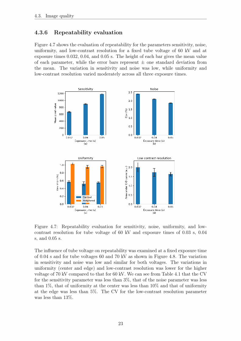
Figure 4.7 shows the evaluation of repeatability for the parameters sensitivity, noise,uniformity, and low-contrast resolution for a fixed tube voltage of 60 kV and atexposure times 0.032, 0.04, and 0.05 s. The height of each bar gives the mean valueof each parameter, while the error bars represent ± one standard deviation fromthe mean. The variation in sensitivity and noise was low, while uniformity andlow-contrast resolution varied moderately across all three exposure times.

Figure 4.7: Repeatability evaluation for sensitivity, noise, uniformity, and low-contrast resolution for tube voltage of 60 kV and exposure times of 0.03 s, 0.04s, and 0.05 s.

The influence of tube voltage on repeatability was examined at a fixed exposure timeof 0.04 s and for tube voltages 60 and 70 kV as shown in Figure 4.8. The variationin sensitivity and noise was low and similar for both voltages. The variations inuniformity (center and edge) and low-contrast resolution was lower for the highervoltage of 70 kV compared to that for 60 kV. We can see from Table 4.1 that the CVfor the sensitivity parameter was less than 3%, that of the noise parameter was lessthan 1%, that of uniformity at the center was less than 10% and that of uniformityat the edge was less than 5%. The CV for the low-contrast resolution parameterwas less than 13%.

23

4.3. Image quality

Figure 4.8: Repeatability evaluation for sensitivity, noise, uniformity, and low-contrast resolution at the exposure time of 0.04 s and for tube voltages of 60 and 70kV.

Table 4.1: Coefficient of variation (%) for sensitivity, noise, uniformity, and low-contrast resolution for four different tube voltage and exposure time combinationsettings.

Exposure setting Sensitivity Noise Uniformity(center)

Uniformity(edge)

Low-contrastresolution

60 kV, 0.032 s 2.09 0.95 4.24 2.66 11.9360 kV, 0.040 s 1.30 0.79 9.39 4.23 12.1070 kV, 0.040 s 1.27 0.65 3.48 2.17 8.6060 kV, 0.050 s 1.08 0.42 3.97 3.16 6.84

24

4.3. Image quality

Figure 4.9 shows the variation in the spatial resolution parameters (spatial frequencyat 10 and 50% of the MTF) at a fixed tube voltage of 60 kV and for exposure times0.04 and 0.08 s. The variations in both spatial resolution parameters were small.The variation in the spatial frequency at 10% of the MTF decreased, while that at50% increased with exposure time. We can see from Table 4.2 that the CV for bothspatial resolution parameters was less than 5%.

Figure 4.9: Variation in spatial resolution across exposure times 0.04 s and 0.08 sfor a fixed tube voltage of 60 kV

Table 4.2: Coefficient of variation (%) for MTF at 10% and 50% for voltage of 60kV and exposure times of 0.04 and 0.08 s.

Exposure time MTF-10% MTF-50%

0.040 s 3.40 2.660.080 s 1.47 4.95

25

4.4. Collimator alignment

4.4 Collimator alignment

Figure 4.10 shows a set of images obtained with the alignment test object for a tubevoltage and exposure time of 60 kV and 0.125 s, respectively. The opaque (dark)areas at the edges of the images are due to unexposed parts of the receptor. Asubjective analysis was performed by looking at the images with the naked eye. Thesize of the opaque areas and the shape of the exposed areas were features lookedat closely. The shape of the exposed central portions in both images confirmed theuse of a rectangular PID. It is seen from Figure 4.10(a) that the the entire surfaceof the receptor was not covered by the field. Even after rotating the PID through180°, the second image obtained Figure 4.10(b) showed similar characteristics, thusindicating that the alignment of the PID with the primary collimator is correct.

Figure 4.10: Images of collimator alignment for test. (a) Image obtained at the 0°position of the PID, (b) Image obtained at the 180° position of the PID.

26

5. Discussion

The purpose of a QA program is to facilitate operators of a dental clinic in obtainingimages of diagnostic quality with minimum exposure of patients and staff to ionizingradiation. My aim with this thesis was to develop ways to improve the QA of IOX-rays systems by implementing quantitative methods of image quality assessmentthat could track changes in the performance of the system more accurately withoutadding a large workload for the clinical staff. A single image receptor and an X-ray machine were used in this study. I implemented and evaluated tests for theimage receptor’s sensitivity, uniformity, noise, spatial resolution, and low-contrastresolution for the combination of the Schick 33 image receptor and a Focus IO X-raytube from GE Healthcare. A semi-quantitative test for the correct alignment of thePID with the primary collimator was also developed.

5.1 Receptor response

The relationship between the recorded incident dose at the receptor and the meanpixel value measured from an ROI at the centre of the image was used to determinethe signal transfer curve of the receptor. Fourier methods in image analysis such asthe approach used to determine the MTF from an image with a sharp edge are basedon the assumption that the system can be approximated to a linear system [32].The signal transfer curve was found to be linear for exposures below the saturationexposure, as seen in Figure 4.1(b). Beyond the saturation exposure, the mean pixelvalues did not change with exposure. This implies that images obtained above thesaturation exposure will all have an identical appearance. Thus, the exposures belowthe saturation exposure point of the receptor was deemed useful or practical for QApurposes.

Separation of the variance in pixel values into components allows the identificationof the dominant noise source in the useful exposure range. The noise model inequation 3.1 is comprised of two components: quantum and structured noise. FromFigure 4.2, it is seen that quantum noise is the principal source of noise, as desiredand constitutes a fraction greater than 70% of the total noise in the useful exposurerange. Nonetheless, the presence of a structured noise component indicates that thevariance in pixel values is not entirely due to the Poisson nature of X-ray produc-tion and detection. Also, it is observed that the fraction of the total noise due tostructured noise increases with dose, while that due quantum noise decreases withdose at the detector.

27

5.2. Image quality

5.2 Image quality

Sensitivity was calculated as the mean pixel value from an ROI placed at the center ofa flat-field image. As seen in Figure 4.3(a), sensitivity increases with exposure. Thevariation in sensitivity from repeated measurements was small with the CV less than3% at all the tested combinations of tube voltage and exposure time. Uniformitywas expressed as a percentage. The lower the value the better the uniformity of thereceptor. The CV of uniformity measured at the center was below 5% for all theexposure settings investigated except at a tube voltage of 60 kV and exposure timeof 0.04 s, where it was about 9%. A similar observation was made for the uniformitymeasured at the edges, where the CV was less than 3% for all the exposure settingsinvestigated except again at a tube voltage of 60 kV and exposure time of 0.04s, where it was about 4% (see Table 4.1). I do not have an explanation for thisdeviation. Routine measurement of uniformity can be helpful to identify changesin sensitivity over the entire receptor’s surface which could not be accounted for bymere random variations in pixel values.

The noise parameter was measured as the CV of the pixel value expressed as apercentage. A more appropriate way to characterize noise in a radiographic imageis by computing the noise power spectrum (NPS) [13]. However, the method used inthis thesis is sufficient for routine QC due to its simplicity. Deviation in noise beyondan acceptable limit may signify changes in the performance of the receptor or theX-ray tube that could not be accounted for by simply randomness in the productionand detection of X-rays photons. Repeatability evaluation showed that the variationin noise was small. The CV was below 1% at all the tested combinations of tubevoltage and exposure time. The area under the C-D curve decreased slightly withincreased in exposure time as seen in Figures 4.5. The smaller the area, the betterthe low-contrast resolution of the receptor. The slight improvement in low-contrastresolution with increase in exposure is perhaps due to a reduction in noise. Thevariation in the low-contrast resolution was moderate with the CV between 6 - 13%.(see Table 4.1).

The presampling MTF was determined from a single slanted edge image. Spatialresolution was measured as the spatial frequencies at 10% and 50% of the MTF.As seen in Figure 4.6, the measured presampling MTF did not change much withexposure settings. However, the effects of other factors in the calculation such as thesize of the ROI for the determination of the ESF and the method used in smoothingthe ESF and the LSF needs to be investigated further. The CV of the spatialresolution parameters was less than 5% (see Table 4.2). The technique used in thiswork offers a simple practical approach for determining the MTF of receptors for IOX-ray imaging. The edge device is easy to fabricate and the method is less prone tophysical imperfections in the fabrication of the device.

5.3 Collimator alignment test

Visual inspection of the PID and primary collimator arrangement with the nakedeye is a common way to check for correct alignment. This approach is subjective

28

5.4. Application to routine QC

and prone to observer variability. The method described in this thesis uses a simpleradiographic test object designed to produce images containing information relatedto the alignment of the collimators. A semi-quantitative evaluation of the imagesobtained using the collimator alignment test objects was straightforward. The largedifference in contrast between an exposed and an unexposed part of the receptor’ssurface in the images makes it easy to determine how much of the receptor’s surfacewas outside of the beam. In the situation of a perfect alignment of the collima-tors, the X-ray field is not supposed to cover the entire surface of the receptor. Anobjective method would be more consistent and suitable. My greatest disappoint-ment was that I did not figure out a method to automate the testing of the images.Further studies should consider how this can be done.

5.4 Application to routine QC

Quantitative assessment of image quality is vital to detect changes in the perfor-mance of the system that may result in degradation in diagnostic image quality. Theinitial step to establish baseline performance values for the image quality parametersused might be time-consuming, but once this is done, subsequent QC testing willbe straight forward. The baseline performance will be used to detect any changesin the system during QC testing. The testing frequency should be such as to ensurereasonable confidence that the system is functioning as expected between tests. Thesensitivity and the noise parameters are sensitive to changes, and therefore needto be monitored more frequently. Meanwhile, uniformity, low-contrast resolution,and the spatial resolution parameters are less sensitive to changes, and thus can betested less frequently. The recommended testing frequency for these tests is givenin Table 5.1.

Table 5.1: Recommended frequency for routine QC testing.

Test Frequency

Sensitivity Weekly or daily.Noise Weekly or daily.Uniformity Monthly.Spatial resolution During acceptance testing of a new sensor or

whenever damage of the sensor is suspected.Low-contrast resolution During acceptance testing of a new sensor or

whenever damage of the sensor is suspected.Collimator alignment Annually and after maintenance of the system.

The QC process can be optimized through the creation of software for automatedanalysis of the acquired images. In this case, the sensitivity, noise, uniformity, andthe low-contrast resolution metrics could all be monitored at the same frequencyfrom a single flat-field image.

29

6. Conclusion

The image quality tests implemented in this work are objective and repeatable.Only two images: a flat-field image and an image of a sharp edge are requiredduring each QC of the receptor. Sensitivity, uniformity, noise, and low-contrastresolution are all determined from the same flat-field image, while spatial resolutionis determined from the edge image. Repeatability of the image quality parametersassessed was found to be acceptable for an automated workflow for QA testing of IOimages. The setup for the assessment of the alignment of the collimators describedin this work is very practical and suitable as part of a routine QC that can limitrepeat examinations. The tests described here were implemented for a specific sensorand X-ray tube combination, but the methods could easily be adapted for differentsystems by simply adjusting certain parameters. Moreover, further work needs tobe done for the present methods to be implemented into a fully automated QAprogram. Future studies should consider the development of a method to automatethe testing of the collimator alignment test images and reproducibility measurementsto ensure consistency of the methods across different sensors and X-ray systems.Also, the long-term consistency of the methods needs to be investigated by acquiringmeasurements over an extended period following a planned timetable.

30

Bibliography

[1] P. van der Stelt, “Better imaging: The advantages of digital radiography,” TheJournal of the American Dental Association, vol. 139, pp. S7 – S13, 2008.

[2] United Nations. Scientific Committee on the Effects of Atomic Radiation,“Sources and effects of ionizing radiation: Sources,” 2000.

[3] J. Valentin, “The 2007 recommendations of the international commission onradiological protection. icrp publication 103.,” 2007.

[4] Sveriges Riksdag, “Strålskyddslag (2018:396),” 2018. [Online; accessed 20-January-2020].

[5] Strålsäkerhetsmyndigheten (SSM), “Strålsäkerhetsmyndighetens föreskrifter omanmälningspliktiga verksamheter ssmfs 2018:2,” 2018.

[6] D. Mondou, E. Bonnet, J.-L. Coudert, M. Jourlin, R. Molteni, and V. Pachod,“Criteria for the assessment of intrinsic performances of digital radiographicintraoral sensors,” Academic Radiology, vol. 3, no. 9, pp. 751 – 757, 1996.

[7] A. G. Farman and T. T. Farman, “A comparison of 18 different x-ray detectorscurrently used in dentistry,” Oral Surgery, Oral Medicine, Oral Pathology, OralRadiology, and Endodontology, vol. 99, no. 4, pp. 485 – 489, 2005.

[8] H. Udupa, P. Mah, S. B. Dove, and W. D. McDavid, “Evaluation of imagequality parameters of representative intraoral digital radiographic systems,”Oral Surgery, Oral Medicine, Oral Pathology and Oral Radiology, vol. 116, no. 6,pp. 774 – 783, 2013.

[9] K. Hellén-Halme, C. Johansson, and M. Nilsson, “Comparison of the perfor-mance of intraoral x-ray sensors using objective image quality assessment,” OralSurgery, Oral Medicine, Oral Pathology and Oral Radiology, vol. 122, no. 6,pp. 784 – 785, 2016.

[10] J. M. Iannucci, Dental radiography : principles and techniques. St. Louis, Mo.:Elsevier Saunders, 4th ed.. ed., 2012.

[11] A. Shetty, F. T. Almeida, S. Ganatra, A. Senior, and C. Pacheco-Pereira, “Ev-idence on radiation dose reduction using rectangular collimation: a systematicreview,” International Dental Journal, vol. 69, pp. 84–97, 4 2019.

[12] J. Hubar, Fundamentals of Oral and Maxillofacial Radiology. Fundamentals(Dentistry), Wiley, 2017.

31

Bibliography

[13] E. Samei, “Performance of digital radiographic detectors : Quantification andassessment methods,” 2001.

[14] B. A. Arnold, Noise Analysis in Digital Radiography. Boston, MA: SpringerUS, 1986.

[15] P. Monnin, H. Bosmans, F. R. Verdun, and N. W. Marshall, “Comparison ofthe polynomial model against explicit measurements of noise components fordifferent mammography systems,” Physics in Medicine and Biology, vol. 59,pp. 5741–5761, sep 2014.

[16] M. J. Yaffe and J. A. Rowlands, “X-ray detectors for digital radiography,”Physics in Medicine and Biology, vol. 42, pp. 1–39, jan 1997.

[17] M. J. Yaffe, P. C. Bunch, L. Desponds, R. A. Jong, R. M. Nishikawa, M. J.Tapiovaara, and K. C. Young, “5. technical aspects of image quality in mam-mography,” Journal of the ICRU, vol. 9, no. 2, pp. 33–51, 2009.

[18] I. A. Cunningham and R. Shaw, “Signal-to-noise optimization of medical imag-ing systems,” J. Opt. Soc. Am. A, vol. 16, pp. 621–632, Mar 1999.

[19] L. W. Goldman, “Principles of ct: Radiation dose and image quality,” Journalof Nuclear Medicine Technology, vol. 35, no. 4, pp. 213–225, 2007.

[20] M. Båth, “Evaluating imaging systems: practical applications,” Radiation Pro-tection Dosimetry, vol. 139, pp. 26–36, 02 2010.

[21] A. Rose, Vision: Human and Electronic. IBM Research Symposia Series,Plenum Press, 1973.

[22] A. E. Burgess, “The rose model, revisited,” J. Opt. Soc. Am. A, vol. 16, pp. 633–646, Mar 1999.

[23] S. E. Reichenbach, S. K. Park, and R. Narayanswamy, “Characterizing digitalimage acquisition devices,” 1991.

[24] E. Samei, N. T. Ranger, J. T. Dobbins III, and Y. Chen, “Intercomparison ofmethods for image quality characterization. i. modulation transfer functiona),”Medical Physics, vol. 33, no. 5, p. 1466, 2006.

[25] P. B. Greer and T. van Doorn, “Evaluation of an algorithm for the assessment ofthe mtf using an edge method,” Medical Physics, vol. 27, no. 9, pp. 2048–2059,2000.

[26] I. E. Commission, “Characteristics of digital x-ray imaging devices - part 1:Determination of the detective quantum efficiency. technical report,” 2003.

[27] A. Burgess, “On the noise variance of a digital mammography system,” MedicalPhysics, vol. 31, no. 7, pp. 1987–1995, 2004.

[28] N. W. Marshall, A. Mackenzie, and I. D. Honey, “Quality control measurementsfor digital x-ray detectors,” Physics in Medicine and Biology, vol. 56, pp. 979–999, jan 2011.

32

[29] E. Samei, M. J. Flynn, and D. A. Reimann, “A method for measuring the pre-sampled mtf of digital radiographic systems using an edge test device,” MedicalPhysics, vol. 25, no. 1, pp. 102–113, 1998.

[30] W. Rasband, “Imagej, u.s. national institutes of health, bethesda, maryland,usa,” http://imagej.nih.gov/ij/, 2011.

[31] JCGM2008, “Evaluation of measurement data - guide to the expression of uncer-tainty in measurement, jcgm 100:2008,” tech. rep., Joint Committee for Guidesin Metrology, 2008.

[32] C. E. Metz and K. Doi, “Transfer function analysis of radiographic imagingsystems,” Physics in Medicine and Biology, vol. 24, pp. 1079–1106, nov 1979.

quality assurance of intra-oral x-ray images

Documents