qualitative comparision of optical and electrochemical sensors for

INSTITUTE OF PHYSICS, CHEMISTRY AND BIOLOGY

MASTER THESIS

QUALITATIVE COMPARISION OF OPTICAL AND ELECTRO-

CHEMICAL SENSORS FOR MEASURING DISSOLVED OXYGEN

IN BIOREACTORS

TOMAS LINDBLOM

MASTER THESIS PERFORMED AT BELACH BIOTEKNIK AB MARS 06 2009

09/2061

SUPERVISOR MARTIN CARLSSON

EXAMINER CARL-FREDRIK MANDENIUS

LINKÖPING UNIVERSITY, INSTITUTE OF PHYSICS, CHEMISTRY AND BIOLOGY, 581 83 LINKÖPING

Abstract

In this master thesis, optical dissolved oxygen (DO) sensors are compared to standard elec-trochemical DO-sensors. The optical sensors are also compared against each other. DO is an important parameter to measure and to control during microorganism fermentation. A DO-sensor needs to fulfill certain criteria, such as; purposive response time, the ability to show accurate and stable readings without drift over time, have the capability to manage several sterilizations and exhibiting membrane fouling resistance. The reference used to test these parameters was an industrially accepted electrochemical sensor. By comparing the two tech-nologies, optical sensors showed similar abilities to perform regarding response time and drift performance during the longer test runs. But the optical sensors showed a better performance during sterilizations, with less drift in raw value. When using electrochemical sensors as a reference, different brands of optical sensor gave different results when testing for accuracy at different concentration levels. Due to error in the method, tests for fouling were inconclu-sive. However, membranes from the two kinds of technologies showed an equal hydrophobic character. The two participating optical DO sensors, Mettler Toledo InPro 6990i and Hamil-ton Visiferm were compared regarding ability to manage sterilizations and generate accurate measuring values at different DO concentrations. The two sensor brands showed an equal behavior during the fifteen test sterilizations. The Mettler Toledo InPro 6990 had better abili-ties to follow the linear behavior of the electrochemical reference sensor. While the Hamil-ton Visiferm sensor differed at most 3.5% units from the electrochemical reference values. Hamilton Visiferm was tested with analogue signal, which gave a noise problem. When using digital signal the noise disappeared. The goal of this study was to recommend a sensor, for Belach Bioteknik AB, and the recommendation would be Hamilton Visiferm, for being prac-tical as well as reasonable priced without renounce of measuring quality.

Table of contents

1. Introduction ............................................................................................................................ 1

2. Background ............................................................................................................................ 2

2.1 Dissolved oxygen and its meaning for fermentation ........................................................ 2

2.2 How to distribute dissolved oxygen ................................................................................. 2

2.3 How to measure and regulate dissolved oxygen .............................................................. 3

2.4 Electrochemical oxygen electrode ................................................................................... 4

2.4.1 Technique .................................................................................................................. 4

2.5 Optic dissolved oxygen sensors ....................................................................................... 5

2.5.1 Technique .................................................................................................................. 5

2.6 Sensor characteristics ....................................................................................................... 6

2.6.1 Electrochemical sensors ............................................................................................ 6

2.6.2 Optical sensors ........................................................................................................... 7

2.7 Other ways of measuring oxygen ..................................................................................... 9

2.8 Contact angle measurement ............................................................................................. 9

2.9 Yeast fermentation ........................................................................................................... 9

2.10 Membrane fouling ........................................................................................................ 10

2.11 Data analysis and factorial trails .................................................................................. 10

2.11.1 T-tests for comparative experiments ..................................................................... 10

2.11.2 Two factorial design for analyze of variance ........................................................ 11

2.12 Purpose ......................................................................................................................... 12

2.13 Method ......................................................................................................................... 12

3. Materials .............................................................................................................................. 13

3.1 Chemicals and consumables........................................................................................... 13

3.2 Equipment ...................................................................................................................... 13

3.3 Software ......................................................................................................................... 14

4. Choice of participating sensors ............................................................................................ 15

4.1 Mettler Toledo, InPro 6990i ........................................................................................... 16

4.2 Hamilton, Visiferm DO .................................................................................................. 17

4.3 Applisens LowDrift dissolved oxygen sensor ................................................................ 18

4.4 Mettler Toledo, InPro 6800 ............................................................................................ 19

5. Methods................................................................................................................................ 20

5.1 Experimental design ....................................................................................................... 20

5.2 Statistical models and air compensation ........................................................................ 20

5.2.1 t-Test ........................................................................................................................ 20

5.2.2 Balanced ANOVA, two factors ............................................................................... 20

5.3 Membrane Performance ................................................................................................. 21

5.3.2 Growth Medium ...................................................................................................... 21

5.3.3 Pre-experiments ....................................................................................................... 21

5.3.4 Fouling ..................................................................................................................... 22

5.3.5 Contact angle measurement ..................................................................................... 23

5.4.1 Experimental setup .................................................................................................. 23

5.4.2 Response time .......................................................................................................... 24

5.4.3 Long run .................................................................................................................. 26

5.4.4 Function test ............................................................................................................ 26

5.4.5 Sterilization .............................................................................................................. 27

5.5 Signal performance ........................................................................................................ 27

5.5.1 Noise and disturbance .............................................................................................. 27

6. Evaluation and results .......................................................................................................... 29

6.1 Membrane performance ................................................................................................. 29

6.1.1 Pre-experiments ....................................................................................................... 29

6.1.2 Fouling ..................................................................................................................... 29

6.1.3 Contact angle measurement ..................................................................................... 30

6.2 Sensor performance ........................................................................................................ 32

6.2.1 Response time .......................................................................................................... 32

6.2.2 Long run .................................................................................................................. 38

6.2.3 Function test ............................................................................................................ 41

6.2.4 Sterilization .............................................................................................................. 43

6.3 Signal performance ........................................................................................................ 45

6.3.1 Noise and signal characteristics ............................................................................... 45

7 Conclusions ........................................................................................................................... 49

7.1 Electrochemical in comparisons with optical dissolved oxygen technology ................. 49

7.2 Mettler Toledo InPro 6990i in comparison with Hamilton Visiferm............................. 49

7.3 Errors in methods ........................................................................................................... 50

8 Further studies ....................................................................................................................... 51

9 Acknowledgement ................................................................................................................ 52

10 References ........................................................................................................................... 53

Appendix A: Results ................................................................................................................ 57

Appendix B: Equipment .......................................................................................................... 59

Appendix C: Methods .............................................................................................................. 60

1

1. Introduction

The biotech industry has a need to measure and control dissolved oxygen (DO) concentration during cultivations of microorganisms. Since the nineteen fifties DO has been measured with electrochemical sensor technology, which gives a value between 0% and 100% of air satura-tion. The technique has had a lot of advantages with a purposive response time, good accura-cy and the possibilities to detect small concentration changes. However, the technology has also disadvantages. Over time the sensor drifts away from its calibration which induces prob-lems in longer fermentations. It has a vulnerable membrane that is easily broken, which stops the oxygen regulation. The membrane gets fouled easily and the sensor needs maintenance relatively often.

All the disadvantages and especially the risk of ending up with a non-functioning sensor have made the industry skeptic. Companies that ferments and measures DO usually works preven-tively and have been changing perfectly workable membranes and electrolytes before every batch, instead of risking the content.

Until recently there has been no competing option to the electrochemical sensors. All other technologies have been too expensive, invasive or have had other problems. During the last decades scientific research has slowly grown regarding optical DO-sensors. For a couple of years ago the first sensors showed up commercially. Nowadays there are a number of compa-nies producing optical DO-sensors for the biotech industry.

Even if the electrochemical sensor has its problems it is essential to know whether or not the new optical sensors can perform equally well, when it comes to the positive sides of the elec-trochemical technology. The industry is also interested in if the optic technology can over-come the problems electrochemical technology has been facing.

The aim of this study was to compare the optical DO-sensor technology with the established DO electrochemical technology. The study focused on parameters important for microorgan-ism fermentation e.g. response time in different fermentation conditions, ability to manage long fermentation times without drift, membrane fouling, ability to manage sterilizations, function tests for different dissolved oxygen concentrations and general observations. Two different brands of optical sensors were tested against one electrochemical sensor and a part of the study was also to investigate which of the sensors were best suited for Belach Biotek-nik AB.

2

2. Background

2.1 Dissolved oxygen and its meaning for fermentation Air contains approximately of 20.95 % oxygen. A fluid can dissolve a certain amount of oxy-gen before it gets saturated. For water this amount is 8.26 ppm (8.6 mg/L) (1). The saturation limit differs depending on pressure and temperature. According to Henrys law solubility of a gas is proportional to its partial pressure. An increase of gas pressure above the water surface will increase the pressure in water equally. If the total pressure increases, so will each indi-vidual gas component. Which means that the partial pressure of oxygen in water will increase and therefore make the saturation limit higher (2). This can be used in fermentation processes to increase growth by supplying organism with more oxygen, when increasing the pressure (3). The solubility of oxygen will also decrease with an increasing temperature (2) and with an increase in salinity (4).

Microorganisms can manage their metabolism either aerobe, with oxygen or anaerobe with-out oxygen. In anaerobic organisms ATP, which is an immediate donor of free energy, is only produced from glucose in glucolysis. If the organism is aerobe it has the capability to process pyruvate, from the glucolysis in the citric acid cycle (Krebs cycle) and finally produce ATP, in oxidative phosphorylation. Therefore, the aerobes can produce more energy and increase growth rate.

The anaerobe organisms are lacking mitochondria and cannot handle oxygen, which then can become toxic. The aerobe organisms, on the other hand, produce toxic products from the py-ruvate when the citric acid cycle do not work (5). In both cases the situation can get trouble-some when oxygen level is too high or too low. The culture risks dying, get inhibited growth or it will stop producing the correct product. There is also a group in-between the aerobe and anaerobe group that requires a low amount of oxygen, called microaerophilic (6).

2.2 How to distribute dissolved oxygen In a bioreactor it is essential to regulate the amount of oxygen to suite the cultivated organ-ism. To do so, regulation equipment is necessary but also the ability to distribute the oxygen for a homogenous oxygen environment.

A large volume of fluid has a limited possibility to exchange oxygen through the surface of the liquid (6). Depending on type of reactor different approaches are used to solve the oxygen distribution problem. In a stirred tank reactor equipment such as spargers, baffles and impel-lers are used. The sparger distributes the oxygen at the bottom of the fermentor. To create a homogenous environment impellers are used. Depending on sensitivity of the fermented or-ganism, different type of baffles, impeller speeds, impeller model and sparger model are used. A mammalian cell culture often needs marine impellers with less sheer force and a low-er impeller speed, down to 120 rpm. They also need a better distribution of small bubbles, from the sparger, because big bubbles that burst can be a threat to the cell structure. A suita-ble sparger would be the perforated pipe ring sparger or a sintered sparger. Baffles can harm

3

the cells so in many cases they are removed. For a less sensitive culture with bacteria cells carefulness can be changed to efficiency (7). Several impellers can be used at high speed, in some cases up to 1900 rpm (8). The impellers are often of Rushton disc turbine type. They break the bubbles into smaller bubbles, which increase the total area of the gas /liquid inter-face. The bacteria can handle the high sheer forces and to further increase fast distribution of oxygen, four baffles are mounted in the reactor and a high flow of oxygen can be applied.

Different alternatives of equipment are combined to gain the best distribution of air, to the aerobic culture without harming the organism (7).

2.3 How to measure and regulate dissolved oxygen It is of great importance to be able to monitor and control the amount of dissolved oxygen as well as adapting it to the organism being fermented. In-line measurement by dissolved oxy-gen probes are commonly used (9).

The oxygen probe is often connected to a control system with possibility to alter the dis-solved oxygen concentration by:

• Altering the temperature. If the temperature is decreased cell activity will slow down and the culture will consume less oxygen (6).

• Increase or decrease the stirring speed. If the stirrer speed is changed so is the distri-bution of oxygen according to chapter 2.2 how to distribute oxygen.

• Limit the amount of added nutrient. This will also decrease the cells activity and pos-sibility to grow (5). Therefore they will consume less oxygen.

• Add extra oxygen to the gas sparged in to the reactor. • Increase pressure to dissolve more oxygen in the same amount of water. According to

the theory in 2.1 Dissolved oxygen and its meaning for fermentation, an increased pressure gives a higher saturation limit for dissolved oxygen.

Even if the sensor has to work in many different reactor environments it still needs ability to produce accurate measurements, to prevent defect and lethal regulation. There are basic pa-rameters that needs to be fulfilled regardless of environmental measuring conditions.

• The sensor probe membrane needs to be able to work in an environment with biologi-cal contents without risking fouling. Hydrophobic membranes reject cell debris and are reducing the risk of fouling. A bio-microfilm can affect the sensor measuring per-formance (10).

• DO-sensors need the ability to detect concentration changes fast enough for the regu-lation system to react, without cell or product damages (11). The need of fast response time depends on the fermented organism. If the sensor is used in a mammalian cell cultivation the changes are slow in comparison to bacterial cultivations were changes happens more rapidly (7).

• Measurement over a long time period must be possible without drifting from the orig-inal calibration. Dissolved oxygen values will be incorrect at the end of the batch if the sensor is drifting from the original calibration (12).

4

• Dissolved oxygen sensor probe needs to measure with enough accuracy to keep the concentration in an optimal concentration interval (13).

• To eliminate contaminations in the reactor sterilization and cleaning in place are used. The sensor needs to be able to handle high temperatures and chemical treatment (43).

Then, there are other factors not directly related to the measurement but still very important. A slim design can be important if the reactor system is small or if there are space problems where the sensor is inserted. It needs to be reliable without risks of contaminating the culture and stop regulation.

Besides from the above mentioned demands it also has to be cost effective with a suitable pursuable price and a low maintenance price.

2.4 Electrochemical oxygen electrode The electrochemical oxygen electrodes have for a long time been the standard instrument for measuring partial pressure of dissolved oxygen in the fermentation industry. The technique also goes under the name Clark Cell electrodes (10).

2.4.1 Technique The electrochemical cell consists of an anode and a cathode. They are in circuit with each other through an electrolyte. The complex forms an electric cell. It contains of ions that react with oxygen and affect the electrical characteristics of the cell. The electrolyte and the anode/cathode are physically isolated and insulated from the surroundings by a membrane. The membrane is permeable to oxygen (14).The enclosing membrane can for example be made of polyethylene with coating of hydrophobic Teflon (15) and the electrolyte can be KCl (4). The cathode is often inert and made of platinum and the anode can be made of silver. The silver anode can also be called the reference electrode (36).

In a polarographic electrode the anode and cathode are polarized from an amplifier, -675 mV. When oxygen penetrates the membrane and reaches the cathode, it gets reduced and simulta-neously there will be a oxidation at the silver anode. This will create a current which will be proportional to the partial pressure of oxygen (16).

The reduction mechanism of oxygen, at the cathode:

O2 + 2H+ + 2e- → H2O2

O2 + 4H+ + 4e-

→ 2H2O

For the silver anode, the oxidation mechanism is:

Ag + Cl− → AgCl + e−

The membrane permeability will change with temperature and has to be compensated for with a built in thermometer or the reactor system thermometer (16).

5

Another type of electrode is the galvanic electrode. It has an anode and a cathode in materials that have electrochemical properties creating a natural potential difference. The difference is big enough to drive the redox reactions and no external potential is needed. The sensor is suitable for low concentration measurement (4).

2.5 Optic dissolved oxygen sensors The optical dissolved oxygen sensor measures the partial pressure with optical technology.

2.5.1 Technique The optical sensor relies on quenching between fluorescent complex, often ruthenium and oxygen. The quenching results in decrease of intensity and change in fluorescence decay life-time (3). Basic components are LED lights, fluorophore complex and a light detecting sensor.

When a LED light illuminate the ruthenium complex, for example tris(4,7-diphenyl-1,10-phenanthroline), electrons in the luminescent molecules will be excitated. Light with low energy will be emitted and picked up by a sensor (for example Si-photodiode).

The fluorophores are usually captured in a gas-permeable and ion-impermeable material such as silicone rubber and included in the optical sensor tip (12) (17).

If there are oxygen molecules on the outside of the silicone, they will penetrate the gas-permeable membrane and get in contact with the ruthenium complex. This will result in re-versible quenching. The oxygen will receive the energy from the excitated electron, which results in heat energy instead of emitting light. It will also cause a time delay before emitting light. The delay and the loss of intensity follow the Stern-Volmer equation from which oxy-gen partial pressure can be gained (12). Like the electrochemical sensors the optical sensor membranes are temperature dependent and have to be compensated for with an internal or external thermometer (18).

Due to photo bleaching of the lumino-phores, modern sensors uses time delay to measure dissolved oxygen concentra-tion (12). A reference light is situated next to the sensor to eliminate tempera-ture drift due to the electronics. The illuminating light often pulses in a given frequency, so the returning emitted light can be presented as a wave. By compar-ing the wave from the emitted light and the wave from the reference light a phase-difference can be detected which will increase proportional to the oxygen partial pressure. A mean value will be used from the phase-difference. The intensity waves and the phase difference can be seen in figure 2-1 (18).

Figure 2-1: The figure shows the phase difference between the reference wave and the measured wave (17).

6

The technique gives a number of possibilities when creating the sen-sor. It is possible to have the detec-tor and the light source far away from the sample and lead the light by optical wires. Another possibili-ty is to have the membrane exter-nal. This means that it is possible to put the membrane with the lumino-phores inside the fermentor, on a glass window and lead an optical fiber to the other side of the win-dow. The illuminating and emitted light pass through the window to the sensing film and the measure-ment does not get invasive. But it is also possible to use the same de-sign as for conventional sensors with the light source and the detec-tor in a steal house illuminating a membrane at the bottom of the sensor, facing the sample liquid (17) (13). By making the membrane, or sensing film thick or small the response time can be controlled. A thin film makes the response time fast and the resolution high, while a thicker film gives less concentration fluctuations due to the slower time to reach equilibrium. The membrane material does also affect response time depending on how fast the oxygen can diffuse over the membrane (3). A sensor with all equipment included in the sensor body can be seen in figure 2-2. The figure also shows the positions of the sensor optics.

2.6 Sensor characteristics

2.6.1 Electrochemical sensors The electrochemical sensors have been industrial standard, for measuring dissolved oxygen since the end of the nineteen fifties. The technique has been the only practical technique, which does not affect the surrounding environment it is measuring, more than consuming oxygen (10).

Electrochemical sensors advantages:

• It measures the oxygen direct and gives a linear response (19).

• It can adapt to changing oxygen concentration fast, with a purposive response time, approximately 60 seconds for a change from zero to 98% of saturation (4).

• It can measure accurate and can detect small changes in concentration. An accuracy of 1% to 2% within the measured value can be expected (19).

Figure 2-2: The figure shows the tip of an optical sensor with the electronics and the luminophores included in a sensor body (17).

7

Electrochemical sensor disadvantages:

• They can easily get ineffective due to fouling of the membrane. When fouling appears medium contents and parts of cells attaches to the membrane and stop oxygen from passing the membrane, making the measurement more insensitive (20) (10).

• For some applications, like fermentation in small bioreactors, the size of the sensor can be a problem (21) (20).

• The membrane is fragile, sensitive and easy to brake. This has led to mistrust from the fermentation industry and they often change the membrane before a new batch (22). If the membrane breaks the sensor will be useless and the electrolyte will leach out from the sensor. Oxygen regulation will be inaccurate and a change of sensor will in most cases lead to contamination (3) (15).

• The sensor is also sensitive to a fluctuating pressure or temperature and has to be re-calibrated if any of the two parameters changes (3).

• The Clark sensor lacks in long terms stability and often drift from calibration. The drift can be a result of aging electrolyte and creation of a surface on the anode. Both the conditions arise due to the properties of the electrochemical cell. This has to be adjusted with recalibration, anode cleaning and change of electrolyte. These three ac-tions are not possible to take under a fermentation process, because the sensor cannot be moved from the cultivation without risking contamination (15) (12).

• Since the sensor contains electronics there is a chance of electrical interference from other parts of the equipment (12).

• When the Clark sensor is not in use, it can only be stored for a couple of months (16).

• The startup time for the Clark sensor is long. It needs to be connected approximately six hours before being fully polarized. If disconnecting the sensor for more than five minutes it needs to be repolarized for six hour (16) (23).

• The Clark sensors needs to be recalibrated after sterilization (16) (23).

2.6.2 Optical sensors The optical sensors differ in advantages and disadvantages depending on how they are built. A lot of building solutions have been tried and several different solutions are available on the commercial market. Therefore a list of general advantages and disadvantages is created. The characteristics for different building solutions are then mentioned bellow.

Optical sensor common advantages:

• The sensors doses not consume any oxygen and therefore it has no effect on the mea-suring environment and does not need continuous liquid circulation (23).

• The temperature response is predictable with the Stern-Volmer equation and it can therefore work in a temperature changing environment (3).

• Small concentration drifts in long runs. The sensor lacks electrolyte and other aging parts. Long runs have been tested in several studies in different environment. In a study by Johnston et al. two electrochemical sensors and three optical sensors were compared during a 30 days test in brackish water. It showed that the optical sensors had less drift from their calibration values (15). Another study by Gao et al. tested

8

optical sensors for 180 days in a cell culture. Two optical sensors were used and no significant drift was detected for 140 days (12).

• Fast or purposive response time (24) (17). Optic sensor response time was tested in a study by Voraberger et al. and the time varied in-between one and two minutes when going from 0% to 90% of saturation (18). Another study by Choi et al. shows re-sponse times of 10 to 20 seconds going from 0% to 100% of saturation. In these stu-dies the sensor was moved from oxygen saturated water to nitrogen saturated water (24). One study reports extra fast response time in low concentrations and accurate measurement down to 6 ppm of oxygen (17).

• Stabile sterilization properties. In a study by Voraberger et al. a sensor was built and tested for ability to manage sterilization. The sensor showed equal measuring value after the sterilization and the conclusion was that no calibration would be needed after sterilization. They also investigated the membrane and could not find any damages from sterilization (18).

• Possibility to long storage time (1). • The technology has a good measuring precision and high sensitivity in small oxygen

changes (17) (19). • The optical sensors have low or no start up times to heat the equipment (1). • The often used LED light source does not harm cells or their products (19).

• Low drift due to fouling. Long runs have been tested in several studies in different environment. In a study by Johnston et al. two electrochemical sensors and three opti-cal sensors were compared during a 30 days test in brackish water. It showed that the optical sensors had less drift because of fouling on the optical membranes in compari-son with the electrochemical sensors (15). Another study by Gao et al. tested optical sensors for 180 days in a cell culture. Two sensors were used and no significant drift was detected for 140 days. In the end of the study fouling did occure (12).

Optical sensors common disadvantages:

• Even if the response time is sufficient it differs when concentration increase and when it decrease. The ruthenium complex has a dissociation constant that is five times smaller than the association constant. This makes response time in decreasing concen-trations slower than for response time in increasing concentrations (19). A report by Glazer et al. measures response time when going from 100% to 0% and back to 100% of saturation. The previously mentioned problem with the fast ruthenium association constant and the slow dissociation constant are shown in the report. Going from 100% to 0% takes 43.3 seconds and going from 0% to 100% takes 8.6 seconds (19).

• The Stern-Volmer behavior makes the signal nonlinear when concentration is changed. It makes the sensor more insensitive at high concentration and the sensor gives a false reading (25). In a study by Hanzon et al. optical sensors were tested against conventional electrochemical sensors in how they correlated in oxygen con-centration. Two sensors had a Pearson correlation of 98.7% and 99.7%. At 30% of sa-turation the sensors differed 5% and at higher concentrations the sensors differed up to 10%. The optical sensor in use had a fluorophore film in the reactor and the optics

9

outside (13). Two other studies by Choi et al. and Glazer et al. confirm the nonlineari-ty at higher concentrations and the loss in sensitivity. They explain it with Stern-Volmer behavior of the sensor (24) (19).

Sensors that uses a sensing film on the inside of the reactor and have the optical equipment on the outside have advantages and disadvantages related to their presumptions. They have no sensitivity to pressure changes and are inert to many chemicals occurring in fermentation (3). Their design that allows electronic equipment to be separated from the sensor gives im-munity to external electromagnetic fields. They are also space conservative.

Optical sensors that uses intensity instead of times shift as a measure of quenching, easily gets problem with photo bleaching, which can give a concentration drift in longer runs. That is not a problem for the optical sensors, using the time shift. They only require readable emit-ted intensity to measure the time shift (26) (25). The negative side of the time shift measure-ment is slower response time in comparison to intensity measurement. Early optical sensors, made of intensity measuring had problem with leakage from the membrane gel, where the fluorophores were situated. This gave problems with drift and changes in response times (27) (28) (29).

2.7 Other ways of measuring oxygen There are other ways of measuring oxygen in liquid. Winklers titration method is one of them, but it is invasive and requires samples taken from the batch. It is accurate and cheap but does not suit the needs of fermentation (24). Chromatographically methods are also poss-ible but expensive, time demanding and require sample from the batch (9).

2.8 Contact angle measurement Contact angle measurement is a widely used method to characterize surfaces hydrophobic preferences. In the method a drop of water is placed on the sample surface. The shape of the drop is controlled of the free energies in the interfaces solid/liquid, liquid/vapor and sol-id/vapor. The topography of the sample also matters for the result. The angle between the tangent of the liquid surface and the tangent of the solid face is called the contact angle. It varies with the shape of the bubble and the shape of the bubble varies depending on how hy-drophobic the sample is. The technique using a water drop is called sessile drop (30).

2.9 Yeast fermentation The yeast cell is fermented in one of two ways. The first option is to ferment the yeast anae-robe. The yeast cells will only be able to produce energy from the glycolysis and the pyruvate will be converted into ethanol and carbon dioxide. For optimal cell growth the second alter-native is used where the yeast is fermented aerobe. With oxygen the pyruvate can be processed and finally turn to energy in oxidative phosphorylation (5). Temperature is another parameter that affects the growth rate. For optimal growth rate the temperature should be around 30oC (31).

10

2.10 Membrane fouling Membrane lifetime and performance are very much dependent on fouling. Fouling is micro-bial and solute adhesion to the membrane surface. One of the toughest fouling agents is bac-teria. They adhere, grow and are very hard to remove from the membrane. Chemicals and disinfection agents are used to clean, which might shorten the membrane lifetime. After three days a membrane is completely covered with a biofilm, when exposed to normal tap water. Cell debris, such as proteins, can also foul a membrane by forming aggregates at its surface.

How well bacteria and other adhesive components foul membranes depends on the membrane material. It is therefore very important to match the membrane materials to the working envi-ronment (32).

2.11 Data analysis and factorial trails Experimental design has to be adjusted to fulfill the purposes of the trials. It is crucial to set up models that can process the generated data to make valid and objective analyses, answer-ing questions concerning the purpose.

When the main objective is to make a comparing study including several different trials, sim-ple basic statistics and modified basic statistics can be used, with randomized design and sev-eral repetitions. After analyzing data the accuracy or validity of the model has to be investi-gated with other tests or visual evaluations, through graphs. The design factors, to be varied during the experiment have to be chosen. They were chosen because of interest gained from previous studies, to focus on the experiment purpose (33).

2.11.1 T-tests for comparative experiments Simple yet powerful statistics can be used to compare a group of values against a static value, one-sample t-test, or two groups against each other, two sample t-test. The t-tests are easy to use and by putting up a statistical hypothesis one can reject or accept the statement that gives information to answer the experiment purpose.

The two sample t-tests are performed on two populations, with equal or non-equal variances. With equal variance one degree of freedom is lost from the test. The loss makes it harder to get the hypothesis rejected but is sometime necessary when the two populations are assumed to have equal variances. Paired t-tests are used when there are differences between the repeti-tions. Means in each repetition are compared against each other, forming a list of differences that are compared against zero.

For the t-tests, certain criteria must be reached to make the test valid. For two sample t-tests the samples must be drawn from two independent populations, the observations must be in-dependent random variables and the variance for the populations has to be equal. If rando-mizing the runs the independence criteria will be fulfilled in most cases. The other two crite-ria can be investigated by putting up a normal probability plot for each population. In the normal probability plot observations are sorted from the smallest to the biggest and plotted against their observed cumulative frequency. If the values in the plot are normally distributed they will end up after an imaginary straight line. The graphical subjective test can be com-plemented with a statistical normality test such as Anderson-Darling in Minitab. If the va-

11

riances are equal the two imaginary lines will be parallel. An example of a normal probability plot can be seen in appendix C, figure C-2.

One sample t-test has equal criteria. The sample must be a random variable from a normal distribution. The assumptions are controlled with a normal probability plot, like the two sam-ple t-tests.

Violations of the assumptions indicate that results from the test might be misleading. It is possible to modify the test, for example, by transformation of the observations.

The power of a test (p-value) represents the least level of significance that would lead to re-jecting the null hypothesis or in other words the smallest α where the data is significant (33).

2.11.2 Two factorial design for analyze of variance When comparing experiment with multiple repetitions the repetition itself can be interesting to involve as a factor. If the repetition affect the main factor of interest, one can see such an influence if adding the repetition as a second factor.

Factorial variance experiments have the advantage of being able to handle many mean values. Factorial variance analysis investigates if the means differ significantly in variance or not, by making f-tests for each of the factors. In this way a factorial variance analyzes can give in-formation about significance in difference for each factor included.

The model for analyzing two factors normally includes a two-factor interaction. If having only one observation per cell (e.g. taking one measurement per sensor, per replicate) the inte-raction can be excluded from the model. When the amounts of observations are equal at each combination, in the factor level, the variance analyzes can be seen as balanced. A balanced analyze gives advantages if the assumption of equal variance is broken (33).

To receive accurate results from the model, certain criteria must be fulfilled. The error has to be normally and independently distributed with mean zero and constant but unknown va-riance. The normality can be investigated with a normality probability plot in the same way as for the t-test. The normality assumption can be a serious threat to validity of the model; however the assumption has to be seriously violated before being a real threat. The indepen-dence assumption is controlled by plotting the residuals in collected time order. If the runs are having positive and negative residuals that indicate positive correlation the assumption is violated. Independence should be achieved by randomized tests and is a serious violation if broken. By plotting residuals versus fitted values one can control the assumption of constant variance, appendix C figure C-2. If patterns are detected in the plotted values there is a risk of no constant variance. A more objective way of determine violation of variance criteria is to make a statistical test for equal variance, appendix C figure C-3. Such a test is Barlett´s test. A balanced model is only slightly affected by non-homogeneity in variance (33).

All tests and controls are easily performed in statistical software such as Minitab.

12

2.12 Purpose The aim of the Master thesis was to map advantages and disadvantages between dissolved oxygen sensors based on electrochemical technology and optical technology. Investigate the possibility to implement the optical technology in Belachs´ present and future equipment and decide which dissolve oxygen sensor best suited for Belach. The comparison was carried out with measurement and practical parameters in focus.

2.13 Method This Master thesis was conducted at Belach Bioteknik AB, Solna Sweden. The market was scanned to find possible optical dissolved oxygen sensor candidates. Literature and articles were studied to investigate which parameters to compare and to find suitable methods. Me-thods from literature were adjusted to suite the test-system and to fulfill the aim of the master thesis. The sensors were compared in capabilities of handling:

• Membrane fouling by exposing membranes for yeast cultivation and determine hy-drophobic performance in a contact angle measurement.

• Changes in concentration by investigating the sensor response time in different fer-mentation environment. Temperature, pressure and agitation were altered in the trials.

• Performance in drift from calibration during a long run conducted for several days. • Several sterilization cycles by looking at response time and change in raw value after

sterilization. • Accurate measurement at different concentration levels.

The results were compared visually and with relevant statistical tools to establish if there were differences and if they were relevant or significant.

13

3. Materials

3.1 Chemicals and consumables Product name Supplier

Nitrogen 5.5 AGA Gas AB, Älvsjö, Sweden

Svenskt strösocker Daniso suger AB, Malmö, Sweden

Potatismjöl Lyckeby Culiner AB, Fjällinge, Swe-den

JO Juice äpple Skånemejerier, Malmö, Sweden

Knorr köttbuljong Unilever Sverige AB, Solna, Sweden

Blå KronJäst Jästbolaget, Sollentuna, Sweden

Test tubes 10mL Terumo Venoject, Leuven, Belgien

Filter papers original Melitta Haushaltsprodukte GmbH & Co. KG, Minden, Germany

YES ORIGINAL Procter & Gamble AB, Stockholm, Sweden

3.2 Equipment Product name Supplier

Fermentor system LARS Belach Bioteknik AB, Solna, Sweden

1-L Fermentor Belach Bioteknik AB, Solna, Sweden

Sensor amplifier CP400 Belach Bioteknik AB, Solna, Sweden

Magnetic stirred heater SR-350 Advantec Toyo, Tokyo, Japan

Scale KEW 6000-1M Kern & Sohn GmbH, Balingen, Ger-many

Rate-Master Flowmeter DWYER instruments, Michigan City, USA

Optical contact angle meter, CAM 200 KSV Instruments LTD, Helsinki, Fin-land

Thermometer pt100 Jumo, Fulda, Germany

Ultrasonic cleaner VWR, West Chester, USA

14

InPro 6990i Mettler Toledo, Greifensee, Switzer-land

Transmitter M400 Mettler Toledo, Greifensee, Switzer-land

InPro 6800 Mettler Toledo, Greifensee, Switzer-land

Visiferm DO Hamilton Company, Bonaduz, Switzer-land

Low dissolved oxygen sensor Applisens, Foster City, USA

3.3 Software Product name Supplier

Biophantom for Optical DO Test v1.00b Belach Bioteknik AB, Solna, Sweden

Minitab 15.1.30.0 Minitab Inc.

Microsoft Office Microsoft

VisiConfigurator V 1.9.157. Hamilton Company, Bonaduz, Switzer-land

15

4. Choice of participating sensors

The market had to be scanned to find suitable sensors. There were a number of manufactur-ers and different kinds of optical sensors to choose in-between. Belach had some basic de-mands on the sensors.

To be able to eventually exchange the old polarographic technology the sensor had to be af-fordable. The purchasing price and the maintenance price had to be reasonable in compare to the polarographic sensors. The sensor had to be fully adapted to the fermentation environ-ment. Being able to cope with sterilizations and the chemicals typically found in a bioreactor. Seven brands were chosen to be further investigated after a first market scan, table 4-1.

Table 4-1: The table shows interesting optic sensors, their equipment and the measurement technology they use.

Brand Equipment Measurement technology Ocean Optics Probe with external light and detector

source

Phase shift and intensity

WPI inc. Probe or sensor film, with external light and sensor source

Phase shift

Tautheta Probe or sensor film, with external light and sensor source

Phase shift

Avantes Probe with external light and sensor source

Intensity

Mettler Toledo InPro 6990i

Probe including optics, with external transmitter

Phase shift

Hamilton Visiferm Probe including all equipment Phase shift PreSens

Probe or sensor film, with external light and sensor source

Phase shift

The brands had a wide variety of features. Techniques from PreSens were interesting because of the possibility to use sensing film on the inside of the reactor and eventually use OEM solutions, which would make it possible to integrate all electronics in the computer and hav-ing a optic cable to the probe in the system computer. However the PreSens alternative was too expensive. Other brands were excluded because of price, size, old technology and bad possibility to support and service. The two sensors chosen for the test were Mettler Toledo InPro 6990i and Hamilton Visiferm DO.

Applisens LowDrift dissolved oxygen sensor was selected as a sensor representing the elec-trochemical technology. Out of the brands Belach uses Applisens LowDrift was the sensor with the best reputation. Three Applisens LowDrift sensors were used. Two electrochemical Mettler Toledo InPro 6800 sensors were also used in the fouling tests, because of delivery delays of Applisens LowDrift sensors.

Totally one Mettler Toledo InPro6990i sensor was used, three Hamilton Visiferm, three Ap-plisens LowDrift low drift and two Mettler Toledo InPro 6800.

16

4.1 Mettler Toledo InPro 6990i The Mettler Toledo InPro 6990i is a sensor with a removable unit containing the electronics such as LEDs, detector and an amplifier. The bottom part of the sensor contains optic fiber to lead light from the removable body to the opto cap. It also contains a thermometer for auto-matic temperature compensation. The O2 selectable membrane in the opto cap is made of silicon. The amplifier sends a digital signal from the removable sensor body to a transmitter (1). The transmitter serves as a control unit with possibilities to alter sensor parameters, con-trol number of sterilization and perform self-diagnostics, for example. The transmitter has several possibilities to send the signal to a computer. In the conducted trials the signal was converted to a 4-20 mA signal (34).

The membrane should be able to manage 50 sterilizations without any problems. Mettler To-ledo InPro 6990i has no general times on membrane life length.

Mettler recommends recalibration after every sterilization/autoclavation and change of opto cap (part with membrane and fluophores). If not using the whole measuring interval Mettler recommends a one point calibration (1). More information about sensor performance can be seen in table 4-2.

According to officials from Mettler Toledo, the feature might offer a solution where the cus-tomer can choose to not use the transmitter but instead receive the digital signal directly to the system computer. However this would require the customer to buy a protocol, to be able to handle the digital signal (35).

Cost associated to the sensor can be seen in table 4-3.

Table 4-2: The table shows sensor characteristics and is a reduced table version from the Mettler Toledo Prod-uct manual for InPro 6880 I (the 6880 i is an older version of 6990 i (1).

Measurement principle InPro 6880 i Permissible pressure range during measurement

0.2...6 bar absolute

Permissible temperature range during measuring

5…60oC

Mechanical temperature resistance -20…130oC Detection limit in: - aqueous medium - liquids containing CO2

8 µg/l [8 ppb] 8 µg/l [8 ppb]

Accuracy: - in aqueous medium - liquids containing CO2

≤ ±[1%+8 ppb] ≤ ±[1%+8 ppb]

Response time at 25 °C (air –> N2)

< 45 s

17

Table 4-3: The table shows costs associated with the InPro 6990 i.

Economics Cost [kr] Purchase costs InPro6880i/120 21 140 :- Transmitter 4300D 19 790 :- Maintenance cost Membrane with opto cap 2 830 :-

4.2 Hamilton Visiferm DO Visiferm is a sensor with built in electronics. The sensor´s body contains of optics, amplifier and the converters needed to send out a digital or analogues signal. The 4-20 mA analogues signal can be directly transmitted to the reactor system. If using the digital signal it can be transmitted to the system computer through a usb-connection. Several Visiferm sensors can be connected through the same usb port. A protocol is needed to translate the signal which is supplied without additional costs. It is also possible to read the sensor through software with ability to calibrate, perform self-diagnostics and manage sensor settings. Software is supplied with the sensor. The sensor has automatic temperature compensation which means that changes in the sensors capability to detect dissolved oxygen, caused by temperature change, is compensated for.

The membrane should be able to manage one year of constant illumination before photo bleaching making it ineffective. Life length of the membrane is somewhere around 50 sterili-zations, depending on environment.

Hamilton Visiferm does not give any specific instructions on when to calibrate the sensor. Calibration can be performed as a two point calibration, in nitrogen and air. It can also be calibrated as a one point calibration in air, depending on sensor use. Before use Hamilton Hamilton recommends a 5 to 10 minutes warm up time (23).

General sensor characteristics can be seen in table 4-4 and sensor economics in table 4-5.

Table 4-4: The table shows sensor characteristics for Hamilton Visiferm dissolved oxygen sensor (23).

Measurement principle Hamilton Visiferm Process pressure

-1...12 bar relative


-10…80oC

Mechanical temperature resistance

-10…130oC

Detection limit in: - aqueous medium - liquids containing CO2

0.01 Vol-% -


- -


< 30 s

18

Table 4-5: The table shows costs associated to Hamilton Visiferm DO sensors.

Economics Cost [kr] Purchase costs Visiferm DO 120 16 480 :- Maintenance cost Membrane with opto cap 3 193 :-

4.3 Applisens LowDrift dissolved oxygen sensor The electrochemical Applisens LowDrift sensor consists of a sensor body housing the elec-trochemical cell. The sensor is polarized by the reactor system amplifier. The current that are occurring from contact with oxygen is sent from the sensor to the amplifier. The sensor does not contain a thermometer and has to be temperature compensated in the computer software with the reactor system thermometer.

The membrane is made out of titanium, possible coating is unknown. Applisens recommends changing membrane after 10 – 15 sterilizations. Applisens recommends calibration after each sterilization and to make a pre-sterilization if it is the first use of the membrane module. The sensor needs to be polarized for six hours before use. If disconnecting the sensor for longer than five minutes the sensor needs six hour of repolarization (16).

General sensor properties can be seen in table 4-6 and economics in table 4-7.

Table 4-6: The table shows measurement characteristics for Applisens LowDrift DO sensor.

Measurement principle Applisens LowDrift Process pressure

Up to 4 bar


-

Mechanical temperature resistance

-

Detection limit in: - aqueous medium - liquids containing CO2

10 ppb


- -

Response time at < 30 s 25 °C (air –> N2) Table 4-7: The table shows costs associated to Applisens LowDrift DO sensors.

Economics Cost [kr] Purchase costs Applisens LowDrift DO 5500 :- Maintenance cost Membrane 750 :-

19

4.4 Mettler Toledo InPro 6800 The technologic setup is equal to Applisens LowDrift, with a sensor body containing an elec-trochemical cell. Contact with oxygen produces an electrical current proportional to the amount of oxygen. The sensor has a built in thermometer for temperature compensation.

Calibration is recommended to be performed after each sterilization and it is important to keep temperature and pressure constant after sterilization. The sensor needs a pre-sterilization for the membrane to get a more constant configuration and to reach a more constant raw val-ue for the following sterilizations. The sensor needs to be polarized for six hours before use. If disconnected shorter than five minutes a shorter polarization time can be applied.

The membrane is made of Teflon and silicon that is reinforced with a steel mesh (36). Sensor characteristics can be seen in table 4-8 and economics in table 4-9.

Table 4-8: The table is a modified copy of a table from InPro 6800 instruction manual (36). Sensor characte-ristics are displayed in the table.

Measurement principle InPro 6880 i Permissible pressure range during measurement

0.2...6 bar absolute


0…80oC

Mechanical temperature resistance -5…140oC Detection limit in: - aqueous medium - liquids containing CO2

6 µg/l [6 ppb] -


≤ ±[1%+6 ppb] -


< 90 s

Table 4-9: The table shows costs associated to Mettler Toledo InPro 6800.

Economics Cost [kr]

Purchase costs Mettler Toledo InPro 6800 10 900 :- Maintenance cost Membrane 548 :-

20

5. Methods

5.1 Experimental design The experiments were divided into three sub groups, each group had its own experimental setup. The first group was to answer if the sensor membranes differed in probability of foul-ing. Three experiments were performed, including pre-experiments, growth on membrane and contact angle measurement. In the second group sensor performance was tested in regard to response time, long run and effects of sterilizations. In the third group sensor signal cha-racteristics were investigated.

Due to delays the optical Mettler Toledo sensor InPro 6990i was not participating in the fol-lowing experiments: fouling, contact angle, pre-experiments and long run.

5.2 Statistical models and air compensation

5.2.1 t-Test Both t-test and paired t-test/two sample t-tests were used. Due to few repetitions, equal va-riance was assumed for the two sample t-test.

For one sample t-tests the difference was investigated for one population with the hypothesis: H0 difference is equal to zero, vs. H1 difference is not equal to zero.

When the mean sensor values comes from repetitions that was equally performed and as-sumed to generate an equal environment, the sensor values could be compared directly against each other. If variations between repetitions were significantly the results could not be trusted. For two sample t-test hypothesis was: H0 no difference between the sensor tech-niques, vs. H1 difference between the techniques. The special form of two sample t-test, paired t-test was used to see if two populations, with different conditions between each repe-tition, differed significantly from each other, also with equal variances.

A third t-test was also applied. The test was used after performing a two factor balanced ANOVA test. The ANOVA test gave information if there were any difference between the repetitions, which meant that repetition dependent variations would be detected. The ANO-VA test also gave a mutual sensor variance. The variance was used in the t-test and the model for the t-test can be seen in appendix C, model 1.

The model was controlled as described in theory section 2.10.1.

5.2.2 Balanced ANOVA, two factors The balanced two factorial ANOVA was used as a way of detecting variances in a sensor group over time, by modifying the factor representing sensor. The second factor was repeti-tions. The ANOVA test made it possible to see if values were dependent on which repetition they came from. The model can be seen in appendix C, model 2.

The model was controlled as described in theory section 2.10.2.

21

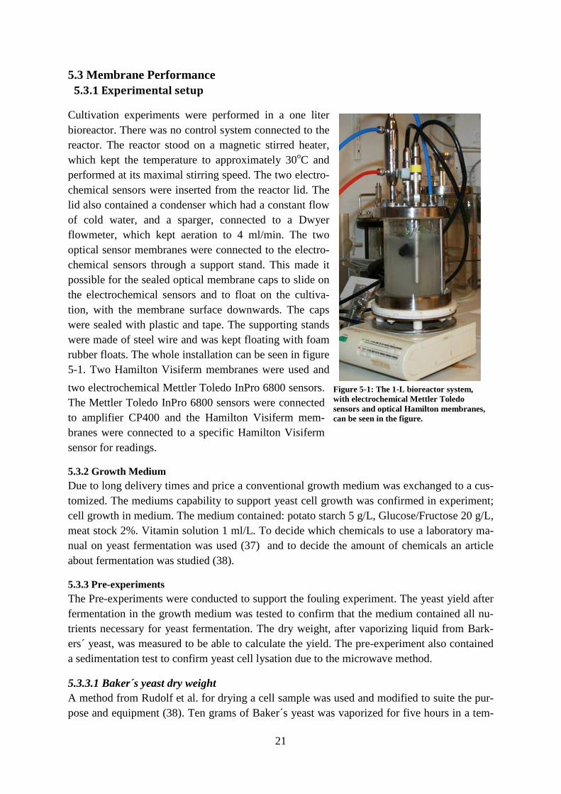
5.3 Membrane Performance 5.3.1 Experimental setup

Cultivation experiments were performed in a one liter bioreactor. There was no control system connected to the reactor. The reactor stood on a magnetic stirred heater, which kept the temperature to approximately 30oC and performed at its maximal stirring speed. The two electro-chemical sensors were inserted from the reactor lid. The lid also contained a condenser which had a constant flow of cold water, and a sparger, connected to a Dwyer flowmeter, which kept aeration to 4 ml/min. The two optical sensor membranes were connected to the electro-chemical sensors through a support stand. This made it possible for the sealed optical membrane caps to slide on the electrochemical sensors and to float on the cultiva-tion, with the membrane surface downwards. The caps were sealed with plastic and tape. The supporting stands were made of steel wire and was kept floating with foam rubber floats. The whole installation can be seen in figure 5-1. Two Hamilton Visiferm membranes were used and

two electrochemical Mettler Toledo InPro 6800 sensors. The Mettler Toledo InPro 6800 sensors were connected to amplifier CP400 and the Hamilton Visiferm mem-branes were connected to a specific Hamilton Visiferm sensor for readings.

5.3.2 Growth Medium Due to long delivery times and price a conventional growth medium was exchanged to a cus-tomized. The mediums capability to support yeast cell growth was confirmed in experiment; cell growth in medium. The medium contained: potato starch 5 g/L, Glucose/Fructose 20 g/L, meat stock 2%. Vitamin solution 1 ml/L. To decide which chemicals to use a laboratory ma-nual on yeast fermentation was used (37) and to decide the amount of chemicals an article about fermentation was studied (38).

5.3.3 Pre-experiments The Pre-experiments were conducted to support the fouling experiment. The yeast yield after fermentation in the growth medium was tested to confirm that the medium contained all nu-trients necessary for yeast fermentation. The dry weight, after vaporizing liquid from Bark-ers´ yeast, was measured to be able to calculate the yield. The pre-experiment also contained a sedimentation test to confirm yeast cell lysation due to the microwave method.

5.3.3.1 Baker´s yeast dry weight A method from Rudolf et al. for drying a cell sample was used and modified to suite the pur-pose and equipment (38). Ten grams of Baker´s yeast was vaporized for five hours in a tem-

Figure 5-1: The 1-L bioreactor system, with electrochemical Mettler Toledo sensors and optical Hamilton membranes, can be seen in the figure.

22

perature of over 100oC. The weight of the dry yeast, after vaporization, was measured on a Kern sr 350 scale. The result was used to make a conversion quote (dry weight/wet weight) to convert a weight of dry yeast to the corresponding weight of yeast and the other way around.

5.3.3.2 Cell growth in medium Approximately 0.1 g of Baker’s yeast (Blå Kronjäst) was added in the 1-L bioreactor, which contained 100 ml of medium. The inoculums were fermented for 24 hours. Another 600 ml of medium was then added and the fermentation kept going for another 72 hours. The method was a modified version of method from Rudolf et al. (38).

The cell suspension was filtered through a filter paper, to exclude clumps of potato starch and medium broth. The suspension was then heated to a temperature over 100oC, for ten hours. After weighing, the fermented dry yeast yield could be calculated by dividing the fermented dry weight with the dry weight of the added amount of yeast. By using the quote from pre-vious dry weight experiment the added amount of dry yeast could be calculated, which could be used to calculate yeast yield.

5.3.3.3 Sedimentation test Two grams of yeast were added and dissolved in a test tube containing 5 mL of water. The procedure was repeated for another test tube which then went through the lysation method. The test tube with unlysated cells and the test tube with lysated cells were compared after 45 minutes. If showing two distinct phases, no or little lysation had occurred. If showing one distinct phase with precipitate and a blurry supernatant, that would indicate lysation (5).

5.3.4 Fouling

5.3.4.1 Lysation Lysation was performed according to protocol in a study from Orsini et al. (39). 7.5 gram of baker´s yeast was microwave, 750 W for one minute.

5.3.4.2 Cultivation Before cultivation, the sensors raw values were read in 30oC air saturated water. Approx-imately two grams of yeast was added to 100 ml of medium in the 1-L bioreactor and the pre-culture was fermented for 24 hours. The two Mettler Toledo InPro 6800 sensors and the two Hamilton Visiferm membranes were inserted to the 1-L bioreactor. Another 600 ml of me-dium was added and the cultivation was fermented for 72 hours. 48 hours into the fermenta-tion 7.5 grams of lysated cells were added to the cultivation, lysation was performed accord-ing to the lysation method. After fermentation the Hamilton Visiferm membranes were con-nected to sensor Ho2. A raw value from each membrane was measured in 30oC of air satu-rated water. The membranes were cleaned and the fouling measurement was repeated. The method came from an article, Johnston et al. but has been modified to the conditions men-tioned above (15). Lysated cells were added to simulate a more fouling promoting environ-ment (33).

23

A total of seven measurements were performed. However, the first measurement was ex-cluded. In the first version of the method, measurement after fermentation was not performed in 30oC air saturated water and therefore gave faulty values.

5.3.4.3 Measurements and statistics The difference between the end value and the air pressure compensated start value was ac-counted for in every membrane and every batch. By using differences for the optical technol-ogy and making mean differences for every batch and then do the same for the electrochemi-cal values, six mean differences for each technology was created, one for each batch. By sub-tracting them against each other six fouling differences between the optical and the electro-chemical technologies were retrieved. These values were used in a one sample t-test to see if they were significantly equal to zero if they differed.

5.3.5 Contact angle measurement Two membranes, from Applisens LowDrift and Hamilton Visiferm, were tested with contact angle measurement. The membranes had previously been exposed to water but had gone through the same conditions. The samples were cleaned in an ultra sonic cleaner, 40 kHz for five minutes in 60oC water. After cleaning, the samples were placed in the contact angle me-ter for measurement. Ten values were measured on both sides of the bubble. Both a receding and an advancing angle were measured. The method was conducted according to an article by Drelich et al. (30).

5.4 Sensor performance

5.4.1 Experimental setup Experiments were performed in water, in a twelve liter LARS-system, figure 5-2. The reac-tor was connected to a computer with regulation software, BioPhantom. Through readings from temperature and pressure sensors the software could PID-regulate those parameters. Stirring speed and aeration could also be monitored and regulated. The stirrer was connected to two Rushton discs impellers, diameter 70 mm, de-signed for bacterial cultivation. The first impeller was mounted one third of the reactor diameter above the reactor bottom and the second impeller was mounted one impeller diameter above the first impeller. For simulating mammalian cell cultivation a marine impeller, diameter 70 mm, placed one third of the reactor diameter above the bottom was used. Four baffles were mounted inside the reactor, at even distances from each

Figure 5-2: The reactor setup with the six sensors in the lid.

24

other. The baffle configuration can be seen in appendix B, figure B-1.

The three Hamilton Visiferm sensors were inserted from the lid and gal-vanically isolated from the rest of the electronic equipment. The three Applisens LowDrift sensors were inserted alternated with the Hamilton Visiferm sensors, in the lid. Two of the Applisens LowDrift sensors were connected to Belachs external amplifiers and one was connected to the system-integrated amplifier. The Mettler Toledo 6990i sensor was also inserted from the lid and connected directly to the LARS electronics. All currents or voltage received by the system were proportionally converted to a raw value in the computer. The raw value was then proportionally converted to a percentage value.

For controlling of dissolved oxygen concentration a gas mixing device was constructed and placed in front of the reactor air inlet. The gas mix-ing unit consisted of closable valves(3), check valves preventing gas from going back to the nitrogen tube or air compressor(2) and a unit combining the two flows(1). The nitrogen flow could be determined with a dwyer rate-master flow meter and the air flow was controlled through the LARS flow meter, controlled from the computer. A description of the gas mix-ing device can be seen in figure 5-3.

5.4.2 Response time

5.4.2.1 Trials In the method from Glazer et al. the sensor is moved from one concentration to a different concentration, through air when measuring response time (19). The sensor risks being af-fected by air when moving in-between the environments. The time it takes to move the sensor will also differ between the trials and affect the measured time. It would also require two reactor systems with equal environments.

The method was altered so the composition of the gas provided to the reactor was changed instead of changing reactor. Depending on stirring speed, flow rate and the reactor design the response time would differ. Response time would include the time to create homogeneity in the system and the sensors ability to detect the concentration change. Therefore the method would not give exact sensor response time. The method was based upon comparison in-between the different techniques.

All sensors were calibrated to have the same dissolve oxygen (DO) concentration values. The concentrations was changed by stopping the 10 ml/min air flow, on the gas mixing device, and open the valve to the nitrogen flow, 10 ml/min. When all sensors had reached two per-cent of DO concentration, the nitrogen flow was closed and the air flow opened. The proce-dure was repeated six times for each test level, table 5-2. All tests were randomize performed.

The response time was read for the following concentrations:

Figure 5-3: Gas mixing device. 1. unit combining Air and N2, 2. valves preventing gas from going back to the N2 bottle or air compressor, 3. valves with abilities to be opened or closed.

25

100% to 75%

100% to 50%

100% to 2%

0% to 50%

0% to 98%

75% to 90%

The response times, regarding decreasing concentrations, were measured from the closeure of the valve controlling air, to when the sensor had reached its DO value. Response times for increasing concentrations were read from the opening of air flow to when the DO value was reached. The opening and closure could be seen in BioPhantom. Low and high levels were chosen to be possible growth conditions covering a broad spectrum, table 5-1. Cultivations has been carried out in higher pressures than 0.75 bar (40), but to avoid going out of sensor measuring range, which would happen at one bar, 0.75 bar was chosen. Atmospheric pressure was chosen as low pressure.

Table 5-1: The table shows the different levels in the three factorial trial.

Parameter Low (-) High (+) Temperature 25oC (41) 400C (41) Pressure(absolute) 0 bar 0.75 bar Agitation 800 rpm (38) 150 rpm* (7)

Table 5-2: The table shows at which test setup the factorial trial response time tests were conducted. + means high level, ex. High temperature and – means low level.* in the low level of agitation the marine impeller was changed to two Rushton disc turbine impellers.

Test setup a=Temperature b=Pressure c=Agitation 1 - - - A + - - B - + - Ab + + - C - - + Ac + - + Bc - + + Abc + + +

To exclude the possibility of misguiding bubble formation due to having water instead of growth medium, surfactants (Yes Original) was added, The results was documented with photos.

5.4.2.2 Measurements and statistics Since there were an equal amount of runs for all factors a balanced two factor ANOVA could be used in mintab. Results from each kind of test, with its six repetitions were inserted to the minitab model to be processed. A variance and an answer if the results were significantly dependent on the batch order was received. The results were then processed according to the test statistics, in appendix c model 1, and the t-test could determine if there were significant

26

difference between the sensor groups. The procedure was repeated for the eight different test setups.

5.4.3 Long run

5.4.3.1 Trials Before the long run, sensors were calibrated to 100% of saturation. During the long run all parameters were kept constant with a temperature of 35oC (41), pressure 0 bar (absolute), aeration 10 mL/min and stirring speed 800 rpm (38), with two bacterial impellers. The sen-sors were calibrated to show 100% of saturation and the fermentor was kept running undis-turbed for 96 hours. The experiment was performed five times. The running conditions were set to simulate a fermention with bacteria or yeast. The method was a time and equipment adapted version from a long run article by Gao et al. (12).

One of the experiments was prolonged to run for 18 days (426 hours) under the same condi-tions as above.

5.4.3.2 Measurement and statistics The results were compensated for varying air pressure.

A balanced ANOVA following model 1, appendix c, was performed. The variance was used to make a t-test to compare the end values between the two groups. The two tests could tell if there were any significant differences correlating to the batch order and if there were any significant changes between technologies regarding the end values of DO.

Two balanced ANOVA tests were constructed to investigate if there were variance difference between the start values and the end values in each sensor group, according to model 2 in appendix c. The tests could answer for if variance changed within each technology over time and if variance differed between the two technologies after a long run. They could also say if there were any significant changes due to the batch order.

5.4.4 Function test

5.4.4.1 Trials In the function test the accuracies of the measured values were tested with the electrochemi-cal Applisens LowDrift sensors as references. All sensors including Mettler Toledo InPro 6990i and Hamilton Visiferm were cleaned and mounted with the reference sensors. The run-ning conditions were set to 35oC, pressure 0 bar(absolute), aeration 10 ml/min and stirring 800 rpm, with the two bacterial impellers. The sensors were calibrated to a hundred percent of saturation. The dissolved oxygen concentration was changed with the gas mixing device, to the following levels 100%, 80%, 60%, 40%, 20%, 0%, 20%, 40%, 60%, 80% and back to 100% of saturation. All sensors had the chance to stabilize on each level. The experiment was repeated for a total of five times and was performed with modifications after an article me-thod by Choi et al. (24). Modifications included a different equipment setup, other oxygen concentration and conditions such as stirring speed.

27

5.4.4.2 Measurement and statistics Paired t-test was constructed to test if there were significant difference between the two opti-cal sensors and the reference sensors at each of the concentration levels. For each of the five tests, mean differences between the optical sensors and the reference sensor were constructed. Minitab was used for the test calculations.

5.4.5 Sterilization

5.4.5.1 Trials All the sensors were connected to the reactor and a calibration with air and nitrogen gas was performed according to each sensors manual (23) (1) (16). Before and after each sterilization a response test was performed, according to the method in response time 5.3.1 and a mea-surement of raw values at 100% saturation was conducted. The sensors were exposed to 121oC for 20 minutes (43) and then cooled down to 35oC. After the each sterilization the temperature on the lid was measured and when reaching 30-35oC the raw values were col-lected. Sterilization method was performed according to article (18).

The lid temperature was not measured before the first sterilization, when raw values were collected. To exclude the lid temperature as an effecting factor of measurement, a raw value measurement at high lid temperature 60oC and low temperature 15oC was performed.

An unsterilized Hamilton Visiferm membrane was tested after fifteen sterilizations, to inves-tigate if a new, unsterilized membrane affected the raw value. The membrane was also ex-posed to a sterilization to see if the sensor performed equally compared to the first steriliza-tion.

5.4.5.2 Measurements and statistics The response times were analyzed with two sample t-tests to make a comparison between the last sterilization and the first sterilization for each technology. If there were significant differ-ences a second two sample t-test were performed, between the first and the penultimate value, until a test showed no significant difference between the response times. With such tests the amount of sterilizations that could be performed without significant change in response time could be determined.

An equivalent test was performed for the raw values. A two sample t-test was used for com-paring raw values before and after the first sterilization, for each technology.

5.5 Signal performance

5.5.1 Noise and disturbance A three seconds digital filter was used on the Hamilton Visiferm signals which can be seen in appendix C. The other two sensor brands were unfiltered.

The noise of the signals were measured by recording the biggest peak-to-valley values in a four minutes run, the sensors were measuring in aerated water. The peak was the maximal percentage value in the noise and the valley was the lowest percent value in the noise, figure

28

5-4. The peak-to-valley value was the percent units in-between peak and valley. Two of the Hamilton Visiferm sensors were compared with and without filter, against the single Mettler To-ledo InPro 6990i and two Applisens LowDrift. The long runs were also scanned for irregular signal behaviors, such as extreme noise or other signal deviations.

Because of the Hamilton Visiferm sensors rela-tively noisy signals, they were connected digi-tally and the sensor signals were read manually in the software VisiConfigurator . The signals peak-to-valley values were read and compared to the analog signal values.

Figure 5-4: Figure shows the definition of peak and valley. The percent points in-between are called peak-to-top value.

29

6. Evaluation and results

6.1 Membrane performance

6.1.1 Pre-experiments

6.1.1.1 Bakers´ yeast dry weight Bakers´ yeast, used for the fouling experiments could after vaporization be characterized to contain 70% water and 30% dry contents.

6.1.1.2 Cell growth in medium After vaporizing the liquid content from the test batch, a dry weight of 2.8 gram was re-ceived. The weight would correspond to approximately 9.6 gram of liquid containing bakers´ yeast.

The inoculums had grown from 0.1 gram of bakers´ yeast to 9.3 gram. A 75-fold cell mass increase proved that the medium contained necessary nutrients for yeast cell growth. Howev-er, even after filtration of the batch content, there was still a risk of having contents from the medium in the filtrate. The medium and cultivation method were proven to be sufficient to be used for the fouling experiments that only require growth of yeast cells.

6.1.1.3 Sedimentation test The test tube with intact cells showed two phases, one containing the precipitate and the other with the superna-tant. The test tube with lysated cells had a blurry superna-tant and less precipitate in comparison with the test tube with intact cells. The right test tube in figure 6-1 contains the intact cells and the left lysated cells.

A qualitative measurement on the amount of lysated cells compared to whole cells could not be performed. Howev-er the results from the sedimentation test together with results from Orsini et al. and Chuanbin et al. implies the microwave method to be workable for the fouling experi-

ments (39) (44).

6.1.2 Fouling The Mettler Toledo InPro 6800 used in this test had been stored for a long time so the electro-lyte was changed and coatings on the anode and cathode were removed. When investigating fouling on the electrochemical Mettler Toledo InPro 6800 sensor membranes and the optic Hamilton Visiferm sensor membranes, a significant difference of oxygen concentration was detected for Mettler Toledo InPro 6800. In the seven batches the first showed extreme values, due to an error in the measuring method. The method was corrected for the following six batches. During the six usable cultivations the Hamilton Visiferm membrane had a mean

Figure 6-1: Test tubes from the lysation experiment. Right tube contains intact cells and the left lysated cells.

30

oxygen concentration increase of 2.50% and the Mettler Toledo InPro 6800 membrane -0.25%, see table 6-1. The Mettler Toledo InPro 6800 difference of -0.25% points was signifi-cant, p=0.01. There was a significant concentration difference between the repetitions, which can have an influence of the results. Due to a high variance the Hamilton Visiferm value was not significant.

The decrease in oxygen concentration was expected because fouling-products would cover the membrane. However an increase of dissolved oxygen was not expected and neither does it correlates with the drift results in the long run. The positive value for the Hamilton Visi-ferm senor is more likely to be the product of an incorrect measurement method. The results for the Mettler Toledo InPro 6800 sensors could be a result of fouling. The experiment could not fulfill the aim of the test, because of probable error in the measuring method for Hamilton Visiferm membranes.

If looking at previous conducted fouling experiments optical membranes has performed bet-ter than the electrochemical. In a 30 days fouling study, by Johnston et al. electrochemical membranes were more exposed to fouling than optical (15).

Table 6-1: Comparisons in between dissolved oxygen raw values before cultivation and, after cultivations. The comparison is made with two membrane of each brand and the percent difference is created from the average difference value of the two membranes.

Batch 1 2 3 4 5 6 Mean Optic difference (%) 4,00% 0,00 % 2,00 % 1,50 % 0,90 % 6,80 % 2,50 % Polarographic difference (%) -1,00 % 1,60 % -0,60 % -1,60 % -3,50 % 3,60 % -0,25 %

6.1.3 Contact angle measurement The Hamilton Visiferm membrane had an advancing contact angle of 104 degrees and the receding was 83 degrees, table 6-2. The angles were mean values of ten measurements and each measurement value was a mean of two angles, measured from each side of the bubble. For the receding angle only angles from the right side of the bubble was used because the bubble interacted with the membrane on the left side and gave false readings. The first value from the receding values is excluded because of an error in the method.

Advancing and receding contact angles were 115 and 70 degrees for the Applisens LowDrift membrane, table 6-2. Since the Applisens LowDrift membrane was curved in both directions it was hard to angle the membrane so the bubble could be applied on a perpendicular surface. The problem resulted in a need of result compensation; five degrees were added on the right side and removed from the left side of the advancing angle. The right side of the receding bubble interacted with the membrane or impurities so only the left side could be used. The membrane shape made processing of the images difficult and only four of the ten images could be processed. That gave an uncertainty regarding the receding angle. The curvature of the Applisens LowDrift membrane can be seen in figure 6-2 and the curvature gives an indi-cation of the need to adapt the baseline to receive the correct angels. Figure 6-3 shows an advancing bubble and a receding bubble on the Applisens LowDrift membrane. It is possible

31

to see how the right side of the receding bubble interacts with the surface while the left side decreases.

Figure 6-2: The Applisens LowDrift membrane under the syringe needle for contact angle measurement.

Figure 6-3: Right side shows an advancing bubble on Applisens LowDrift membrane, left side shows a receding bub-ble on an Applisens LowDrift membrane.

Table 6-2: Receding and advancing angel values for Applisens LowDrift and Hamilton Visiferm membrane in contact angle measurement.

The true contact angle value was somewhere in-between the advancing and the receding an-gle. Values over 90 degrees can be classified as hydrophobic. Because of the uncertainty of Applisens LowDrift receding angle more importance was put into the advancing angle.

Brand Technique Angle [degrees] Hamilton Visiferm Advancing 104 Receding 83 Applisens LowDrift Advancing 115 Receding 70

32

The Applisens LowDrift advancing angle was greater than Hamilton Visiferm´s. However, the difference is small and the hydrophobic character is close to equal.

The almost equal contact angle indicates that fouling should have an equal chance to occur on both the sensors. The individual shape and the fact that one of the technologies has a more active diffusion of oxygen over the membrane might also affect the possibilities of fouling.

6.2 Sensor performance

6.2.1 Response time

6.2.1.1 Concentration change 100% to 75% of saturation When the concentration changed from 100% to 75% of saturation and impeller speed was 800 rpm with Rushton disc turbine impellers, the Hamilton Visiferm had the fastest response time (1, a, b and ab). In the other trials (ac, bc, abc but not in c) that had a lower impeller speed and marine impeller, Applisens LowDrift was superior, figure 6-4. It was in the runs with high impeller speed and Rushton disc turbine impellers (1, a, b and ab) that any signifi-cant difference between the sensor groups could be detected, with power 0.1 or better, table 6-3. The model was violated in two trials (1, ab).

Three of the trials showed no significant concentration changes between the batches (c, ac and abc), while the other trials had significant difference. The results makes the significant difference mentioned above unsecure.

Response time for Mettler Toledo InPro 6990i was tested in one trial with condition one, re-sults can be seen in Appendix A, table A-1. Mettler Toledo InPro 6990i had a response time of 27 s when going from 100% to 75%, which was slower in compare to Applisens LowDrift 25 s and Hamilton Visiferm 23 s.

33

Figure 6-4: Shows mean response times, for six repetitions at each level, for Applisens LowDrift(Ap) and Hamilton Visiferm(Ho) sensors when concentration was changed from 100% to 75%.

Table 6-3: The table shows if there was significant difference between group means in the response time test, 100 to 75% of saturation. The table also presents power for the tests and if the model requirement were satis-fied.

100% to 75%

State Significant difference, group mean Power, P Acceptable model

1 Yes 0,000 Yes

a Yes 0,005 No

b Yes 0,001-0,005 Yes

ab Yes 0,001-0,005 No

c No 0,1 Yes

ac No 0,1 Yes

bc No 0,025 No

abc No 0,1 Yes

6.2.1.2 Concentration change 75% to 90% of saturation The response time trials when changing concentration from 75% to 90% of saturation reveals Applisens LowDrift to be faster in all trials except from b where the times were equal, figure 6-5. There were significant differences in five of the trials (1, a, ab, bc and abc), table 6-4.

0

50

100

150

200

250

Re

spo

nse

tim

e,

sResponse time, 100% to 75%

1 Ho

1 Ap

a Ho

a Ap

b Ho

b Ap

ab Ho

ab Ap

c Ho

c Ap

ac Ho

ac Ap

bc Ho

bc Ap

abc Ho

abc Ap

34

The model was violated, because of non-normal distribution in two trials (1 and ab). The powers of the tests were 0.2 or better.

All trials had concentration dependence, depending on batch order. This gives uncertainty to the significances accounted for the trials.

Response time for Mettler Toledo InPro 6990i, going from 75% to 90%, can be seen in Ap-pendix A, table A-1. The table shows a slower response time for Mettler Toledo 6990i with 27 s, in comparison to Applisens LowDrift 22 s and Hamilton Visiferms 23 s.

Figure 6-5: Shows mean response times, for six repetitions at each level, for Applisens LowDrift(Ap) and Hamilton Visiferm(Ho) sensors when concentration was changed from 75% to 90%.

Table 6-4: The table shows if there was significant difference between group means in the response time test, 75% to 90% of saturation. The table also presents power for the tests and if the model requirement were satis-fied.

75% to 90%

State Significant difference, group mean Power, P Acceptable model

1 Yes 0,01-0,05 No

a Yes 0,005-0,01 Yes

b No 0,1 Yes

ab Yes 0,005 No

c No 0,1 Yes

ac No 0,1-0,2 Yes

0

100

200

300

400

500

600

700

Re

spo

ns

tim

e,

s

Response time, 75% to 90%1 Ho

1 Ap

a Ho

a Ap

b Ho

b Ap

ab Ho

ab Ap

c Ho

c Ap

ac Ho

ac Ap

bc Ho

bc Ap

abc Ho

abc Ap

35

bc Yes 0,05 Yes

abc Yes 0,10 Yes

The Hamilton Visiferms had shorter response times when going from high to low concentra-tions and the Applisens LowDrift was superior in going from low to high concentration. Even if showing significant differences in most trials with high impeller speed with Rushton disc turbine impellers, the differences are small. For biological applications the two to three seconds difference would have a small impact. It is only when impeller speed decreases and using marine impeller that differences gets troublesome, up to 100 seconds. The difference between the replicates gives uncertainty to the statistics. So if comparing response times, from a biological point of view, when varying temperature, pressure and stirrer speed with impeller type, temperature and pressure has no or little impact.

Hamilton Visiferm sensors have a three seconds filter which delays the signal with approx-imately three seconds. With a digital transmission of the Hamilton Visiferm signal no filter would be needed and the response time would in many cases change to Hamilton Visiferms benefit.

The coating for Hamilton Visiferm probably contains of ruthenium complex. Oxygen has a five time faster association constant to ruthenium in comparison to the association constant (19). The feature is delaying the response time when oxygen concentration increases. How-ever the behavior explained in the theory was not seen in the trials. If looking in appendix A table A-1, one can see that the Hamilton Visiferm was ten seconds faster going from 100% to 2% than going from 0% to 98% in trial a. Applisens LowDrift had no time differences. The reason why Hamilton Visiferm was performing different than the theory implies has to be further investigated.

The stirring speed with respective impeller type seems to have a big influence on the oxygen distribution but also on how the sensor groups differ against each other. Over 100 seconds difference can be seen in figure 6-5 in comparison to a few seconds difference in trials with stirring of 800 rpm. The difference can be subscribed to sensor characteristics. Figure 6-6 shows an example of a run with all six sensors, stirrer speed 800 rpm and figure 6-7 shows a run with the same presumption except from the stirrer speed and impeller 150 rpm and ma-rine impeller. If compare the two figures the sensors do not have the same behavior when the stirrer speed is low, with marine impeller, as when impeller speed is fast, with Rushton disc turbine impellers. The marine impeller and slower speed shows a greater variance due to the formations of air bubbles under the sensors. With a large variance the statistical model turns insensitive and cannot obtain sufficient power to the trials, unless there are major differences. The large variance can also give the model problem to reach the requirement of equal va-riance.

The relative big variance was probably due to air bubbles gathered under the membrane. Bubbles stops, water, containing dissolved oxygen, to reach the sensor. In figure 6-8 a Hamil-ton Visiferm sensor with air bubbles gathered under the membrane can be seen and in the

36

same figure there was an Applisens LowDrift sensor with the same problem. The Applisens LowDrift sensor membrane was covered in a bubble and with such bubble present the sensor gets insensitive to concentration changes. When the bubble moves, the signal adapts to the new concentration. The Hamilton Visiferm sensor has several smaller bubbles and liquid can reach the membrane between the bubbles. The high values from the contact angle measure-ment can be a reason why there are bubbles. The highly hydrophobic membranes reject polar water but will welcome inert nitrogen, which is the main component in air. The Applisens LowDrift faster response time in almost all experiments with low impeller speed and marine impeller can be a result of fewer bubbles under the membrane. The arched membrane shape can be a beneficial property for getting the bubbles to slide of the membrane.

Since the experiments were carried out in water, a different surface tension could be expected in a medium containing microorganisms (42). A lower surface tension would result in smaller bubbles and the bubble problem might be negligible. To get an indication if surfactants would make the problem disappear detergent was added and the membrane was photographed, fig-ure 6-9. There are several small bubbles but the larger bubbles were still there and after some time they increased in size. This problem can probably be expected in cell cultivations.

Figure 6-6: The figure showes a example of response time run when agitation was 800 rpm and Rushton disc turbine impeller. Hamilton Visiferm(Ho) and Applisens LowDri ft(Ap) are participating.

37

Figure 6-7: Illustrates one of six response time runs with low impeller speed, 150 rpm and a marine impeller. Hamil-ton Visiferm(Ho) and Applisens LowDrift(Ap) are part icipating.

Figure 6-8: Left figure shows Hamilton Visiferm and right figure shows Applisens LowDrift sensor.

38

Figure 6-9: Figure shows a Applisens LowDrift membrane when surfactants have been added.

6.2.2 Long run The first runs revealed an irregular concentration pattern, figure 6-10 left side. Dissolved oxygen (DO) values for the six sensors varied synchronous on both sides of the start concen-tration. The same type of pattern was observed in the four following runs. Varying air pres-sure was suspected to influence the measurements. The sensors were not compensated for air pressure and varying DO-concentration in water could be a result of the air pressure. Air pressures from SMHI, Bromma airport were used to make a factor to compensate for differ-ing air pressure. With compensation the irregular pattern disappeared and the test became independent of changes of air pressure, figure 6-10 right side.

Figure 6-10: To the left: Long run number one with uncompensated Hamilton Visiferm(Ho) and Applisens Low-Drift(Ap) mean values.To the right Long run number one with compensated Hamilton Visiferm(Ho) and Applisens LowDrift(Ap) mean values.

By comparing the first DO value with the last value in each group of sensors, in all runs the negative drift could be determined. The mean difference for optic sensors was -1.8 percen-tage points and the mean differences for the electrochemical sensors were -1.6% points. A 96 hour batch gives a negative drift between -1.6% and -1.8% points for the two technologies.

39

The difference between the groups, 0.2% points was not significant, power better than 0.25. There was a significant difference between the batches which might influence the results in this test. A combined graph for the five long runs can be seen in figure 6-11. In the end of the run there was a concentration decrease. The drop in concentration, at day eight, arises be-cause the sensors were used for reading the fouling membranes, but were then reapplied to the batch.

An indication if the sensors were drifting relative to each other was given by comparing the variance in each sensor group. The group variance in the beginning of the batch was com-pared to the variance for the same group at the end of the batch. The optic sensors differed significant in variance after 96 hours of cultivation, p=0.005. However the difference in-between batches was also significant, p=0.007 which can influence the test. Electrochemical sensors had no significant difference in variance, p=0.09 but a significant difference between batches, p=0.007. The model for both the tests was violated regarding the equal variances. Nevertheless, the sample sizes were equal so the variance condition was less important, but could affect the results.

The comparison of mean values implied small differences between the two sensors. This was confirmed by the visual graph results but also by the statistical results. The difference in va-riance can be a result of signal noise which will be further discussed in noise and signal cha-racteristic 6.3 the almost equal negative drift can be the product of lime or biological film fouling on the membranes. A covering, that could be lime, was often seen on the membrane and bacteria from tap water can foul membranes. It could also be a signal related problem. If being signal related the problem was most likely in the system and not in the sensors which does not share the same technology with each other.

According to results from other studies, by Gao et al. and Johnston et al., the optic technology should be relatively undisturbed by drift during longer runs (12) (15). That does not exclude signal error or fouling.

Figure 6-11: Shows all five long runs in a combined plot with mean values for Hamilton Visiferm(Ho) and Applisens LowDrift(Ap).

40

As an indication of the sensor behavior in a longer run, the fifth run was prolonged to approx-imately 18 days (426 hours). The run can be observed in figure 6-12 and an air and a pressure compensated run with the group means can be seen in figure 6-13. The run reveals two signal characters for the optical sensors, a sudden drop of DO-concentration and noise. These two characteristics will be further investigated in 6.3.1 Noise and signal characteristics. Because figure 6-13 shows mean values and has a low resolution the concentration drop and the noise are less observable in that figure.

The difference between the end-values of the two groups was 0.6% points and a comparable difference could also be seen in the 96 hour runs. Time does not seem to make the sensors differ from each other. However if looking at the compensated graph a negative drift for the two groups of approximately 7.5% points can be observed. The 4.5 fold increase of cultiva-tion time has generated a 4.5 fold increase of the negative drift. The drift pattern could be interpreted as almost linear over time. The same explanations could be adopted for the longer run, as for the shorter regarding the drift.

Figure 6-12: Long run five with all participating sensors (Mettler Toledo InPro 6990i(Mo), Hamilton Visiferm(Ho) and Applisens LowDrift(Ap))

41

Figure 6-13: Long run number five with Applisens LowDrift(Ap) and Hamilton Visiferm(Ho) mean values compen-sated for air pressure changes.

6.2.3 Function test The Hamilton Visiferm sensors differed significantly from Applisens LowDrift in all concen-tration levels except from 100% and 0%, table 6-5. Figure 6-14 shows how much InPro 6990i and Hamilton Visiferm differ at each concentration level which was especially obvious in the concentration range 20%-60%, both in the decrease of concentration and the increase. At 40% the difference was as much as 3.5% points. Mettler Toledo InPro 6990i followed the reference sensor Applisens LowDrift with small differences, often around 0.2% points. There were no significant differences between the sensors. Due to the small differences and big, variances the tests powers were weak often 0.7.

Table 6-5: The table shows if there was significant difference between Applisens LowDrift/Hamilton Visiferm and Applisens LowDrift/Mettler Toledo InPro 6990i in the function tests. The table also presents power for the test and if the model requirement of normal distribution was satisfied.

Percent of saturation [%]

Significant differ-ence between Appli-sens LowDrift and Hamilton Visiferm

Power, P

Acceptable model

Significant differ-ence between Ap-plisens LowDrift and Mettler Toledo InPro 6990i

Power, P

Acceptable model

100 No 0,000 Yes No 0,000 Yes

80 Yes 0,01 Yes No 0,7 Yes

60 Yes 0,000 Yes No 0,3 No

40 Yes 0,000 No No 0,3 Yes


0 No 0,2 Yes No 0,09 Yes


42


60 Yes 0,000 Yes No 0,7 No

80 Yes 0,004 Yes No 0,8 No

100 No 0,4 No No 0,5 No

Figure 6-14: Function test, run number five. Electrochemical sensors from Applisens LowDrift(Ap) and optical sen-sors from Hamilton Visiferm(Ho) and Mettler Toledo InPro 6990i(Mo) are exposed for different dissolved oxygen concentrations. The plot is made of mean values from five runs.

Figure 6-15: The difference between electrochemical (Applisens LowDrift) and optical sensors (Hamilton Visiferm and Mettler Toledo InPro 6990i) can be seen during different DO-concentrations.

Low numbers of test repetitions can be the reason why the test of the normal distribution of-ten was failed and the model not accepted. However figure 6-15, showing sensor difference, gives a strong indication that the significances are correct. The irregular pattern of Mettler Toledo InPro 6990i in figure 6-15 can be a result of only using one sensor. The pattern of

0

0,5

1

1,5

2

2,5

3

3,5

4

10

0%

80

%

60

%

40

%

20

%

0%

20

%

40

%

60

%

80

%

10

0%

Dif

fere

nce

. %

po

ints

Percent of saturation, %

Differens between optic sensor and reference

Difference

Applisens/Hamilton

Difference

Applisens/Mettler

Toledo

43

Hamilton Visiferm was much more regular, maybe because it was the mean value of three sensors.

The difference between Hamilton Visiferm and the two other sensors cannot be described in a satisfying way. The identical technologies being used in Hamilton Visiferm and Mettler To-ledo InPro 6990i should give them the same behavior, if they weren’t compensated. It will be a decision for the buyer to decide if the 3.5% point difference between the accepted technolo-gy and the Hamilton Visiferm optical technology can be accepted.

From results presented in earlier studies, such as Choi et al., Glazer et al. and Hanson et al. optical sensors tends to differ at higher concentrations (24) (19) (13). They have explained it with the Stern-Volmer equation. However, the Hamilton Visiferm sensor returns to a correct value at the highest concentration and Mettler Toledo InPro 6990i do not show the behavior at all. Results from a study comparing different oxygen levels in hybridoma and CHO culti-vations showed that it was important to have accurate and sensitive sensors for concentrations under five percent. For product quality the sensor had to be functional over the whole 0% to100% of saturation spectra. Differences of up to ten percent units could be accepted if it did not occur in the lowest concentration spectra. That argumentation would make a 3.5% unit difference, at 40% of saturation, accepted (13).

6.2.4 Sterilization When comparing the response times, 100% to 50%, before sterilization and after 15 steriliza-tions significant difference could be detected for optical Hamilton Visiferm sensors and elec-trochemical Applisens LowDrift sensors. The electrochemical sensors from Applisens Low-Drift could handle 12 sterilizations before the response time differed significantly from the initial time, p=0.09. The optical Hamilton Visiferm sensors showed an equal performance, p=0.11. A variance could not be accounted for Mettler Toledo InPro 6990i since the study only contained one sensor. Without a variance, a statistical test could not be performed on the Mettler response time. However, if assuming a small variance, a visual inspection of fig-ure 6-16 indicates that the Mettler would be able to perform at least twelve sterilization cycles.

The extreme values shown in sterilization three are probably a result from an error in the experimental setup, for example wrong stirrer speed. Therefore, sterilization three is excluded from the calculations.

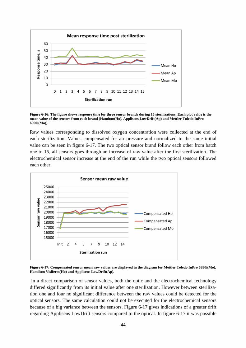
44

Figure 6-16: The figure shows response time for three sensor brands during 15 sterilizations. Each plot value is the mean value of the sensors from each brand (Hamiton(Ho), Applisens LowDrift(Ap) and Mettler Toledo InPro 6990i(Mo)).

Raw values corresponding to dissolved oxygen concentration were collected at the end of each sterilization. Values compensated for air pressure and normalized to the same initial value can be seen in figure 6-17. The two optical sensor brand follow each other from batch one to 15, all sensors goes through an increase of raw value after the first sterilization. The electrochemical sensor increase at the end of the run while the two optical sensors followed each other.

Figure 6-17: Compensated sensor mean raw values are displayed in the diagram for Mettler Toledo InPro 6990i(Mo), Hamilton Visiferm(Ho) and Applisens LowDrift(Ap).

In a direct comparison of sensor values, both the optic and the electrochemical technology differed significantly from its initial value after one sterilization. However between steriliza-tion one and four no significant difference between the raw values could be detected for the optical sensors. The same calculation could not be executed for the electrochemical sensors because of a big variance between the sensors. Figure 6-17 gives indications of a greater drift regarding Applisens LowDrift sensors compared to the optical. In figure 6-17 it was possible

0

10

20

30

40

50

60

0 1 2 3 4 5 6 7 8 9 10 11 12 13 14 15

Re

spo

nse

tim

e,

s

Sterilization run

Mean response time post sterilization

Mean Ho

Mean Ap

Mean Mo

15000

16000

17000

18000

19000

20000

21000

22000

23000

24000

25000

Init 2 4 5 7 9 10 12 14

Se

nso

r ra

w v

alu

e

Sterilization run

Sensor mean raw value

Compensated Ho

Compensated Ap

Compensated Mo

45

to see a decrease after sterilization four and the new value was almost equal to the value after sterilization one. The same tendency can be observed after sterilization nine. The drops in raw value were related to a new day and there had not been any measurement for at least twelve hours. The electrochemical sensors seem to be drifting more than the other two and do not go back the whole way to the value corresponding to sterilization two.

After detecting the rise in raw value after the first sterilization temperature was registered in the steel lid, housing the sensors. The lid temperature was kept constant during the following measurement. To exclude the possibility that the first measurement was a product of high or low lid temperature, different lid temperatures were tested but the raw value staid constant at approximately 20 000 units. An unsterilized Hamilton Visiferm membrane was also tested on one of the sensors to investigate if the sterilization had affected membrane features. The new membrane also gave a raw value around 20 000 units. After sterilization the new membrane still showed 20 000 units. This would indicate that the membrane had nothing to do with the increase of raw value. Since the two technologies differ a lot in design it is tempting to desig-nate the difference to a change in medium. However the medium was exposed to air during measurement after every sterilization and had the same temperature, which make it an unlike-ly source of error. The source of raw value increases has not been located, for the optical sen-sors. For the electrochemical sensors the rise in raw value can probably be subscribed to the electrolyte (16). Gas in the electrolyte disappears when sterilizing and the raw value increas-es. Why the Hamilton Visiferm and Mettler Toledo InPro 6990 shows the same behavior without the electrolyte and when membrane changes can be excluded, has to be further inves-tigated.

Test showed that there were possibilities to use the optical and electrochemical sensors for at least twelve sterilizations without having significant differences in response times. It would also be possible to make the sensor calibration before sterilization without the need of another calibration afterwards, given that it was not the first sterilization or the electrolyte has been changed. Even if the raw value increase with sterilization the sensors can still perform with-out risking going outside the signal range. Over time the increase of raw value can be a prob-lem and the Applisens LowDrift sensors indicate the biggest risk of drifting while the optical sensors stays on a constant value. However, the differences were not significant and could be stopped and restored with a change of electrolyte. The increase seems to be related to the sensor more than the membrane. The suspicion is strengthened by the constant value after changing Hamilton Visiferm membrane to a new unsterilized. The general trend corresponds to an earlier study of sterilizations by Voraberger et al. (18).

6.3 Signal performance

6.3.1 Noise and signal characteristics The signals from the sensors differed in noise. The noise was studied for three Hamilton Visi-ferm sensors, two Applisens LowDrift and the Mettler Toledo InPro 6990i sensor in a fully oxygen saturated, four minutes batch. While the Applisens LowDrift sensor differed approx-imately 0.2% points from highest peak to lowest valley, the Mettler Toledo InPro 6990i dif-fered 0.75% points. The Hamilton Visiferm sensors had the biggest noise with a peak to val-

46

ley variation of 2.8% points. A three seconds filter was tried on the Hamilton Visiferm sen-sors, the noise was reduced to 1.6% points. The signals can be seen in figure 6-18 and the results in table 6-6.

Table 6-6: Describes maximal peak to valley noise for test sensors.

Sensor Peak to valley value Peak to valley value filtered Applisens LowDrift 0.2% points Mettler Toledo InPro 6990i 0.75% points Hamilton Visiferm 2.3%-2.8% points 1.6% points

The noise for Hamilton Visiferm was more than ten times greater compared to the Applisens LowDrift and more than three times compared to the Mettler Toledo InPro 6990i. In long run five a peak-to-valley value of 18% points was observed for Hamilton Visiferm sensor three (Ho3). Sales officials and technicians at Hamilton confirmed the noise to be unusually high. Belach employees tried to locate interfering equipment units to eliminate induced electrical currents from the equipment. No such units could be found. Technicians from Hamilton also tried to locate the source of error. Hamilton personnel expect the problem to be situated in the sensor digitizer.

Since the sensor was connected analogues to the measuring equipment another setup was tried. The sensor was connected digitally to the computer and a Hamilton produced software was used to read the sensors. The signals can be seen in figure 6-19. The signal from Hamil-ton Visiferm one (Ho1) has a peak to valley value 0.3% points, Hamilton Visiferm two (Ho2) 0.3% points and Hamilton Visiferm three (Ho3) 1.0% point. The results were more compara-ble to the Applisens LowDrift and Mettler Toledo InPro 6990i sensors and indicate an error in the analogues transfer or conversion of the dissolved oxygen signal.

The noise for sensor Ho3 was about three times larger in the analogue mode than the noise for sensor one and two. This was not further investigated but it could be a result of new soft-ware or hardware in the sensors. All three sensors membranes were new when starting the tests and have been going through the same treatments.

47

Figure 6-18: Diagram describes the noise of the sensors Mettler Toledo InPro 6990i(Mo), Applisens LowDrift(Ap) and Hamilton Visiferm (Ho).

Figure 6-19: Hamilton Visiferm(Ho) sensor 1, 2 and 3 are tested for 102 seconds with digital connection and software.

The sudden decrease of dissolved oxygen concentration in run number five, figure 6-19 was a phenomena occurring for the three Hamilton Visiferm sensors during the whole test period. One sensor decreased in dissolved oxygen concentration until it reached approximately 10%

98,8

99

99,2

99,4

99,6

99,8

100

100,2

100,4

100,6

0 6

12

18

24

30

36

42

48

54

60

66

72

78

84

90

96

10

2

Pe

rce

nta

ge

of

satu

rati

on

, %

Time, s

Digital reading of Visiferm sensor

Ho1

Ho2

Ho3

of saturation. After reaching 1(100%) again, figure 6-20. Going from fully saturated and back to fully saturated again approximately 20 seconds. Since the other optic and electrochemical sensors did not change in dissolved oxygen can be excludeseconds filtering. The sensors aremeans that other electric parts in the equipment should nproblem was not localized durinor the sensor itself could be excluded as a source to the problem and has to be further invetigated.

Figure 6-20: A concentration decrease for Hamilton

48

of saturation. After reaching 10% concentration value increased showiGoing from fully saturated and back to fully saturated again Since the other optic and electrochemical sensors did not

ssolved oxygen can be excluded. The shape of the curve was a result of the three The sensors are galvanic isolated from the rest of the equipment which

means that other electric parts in the equipment should not influence the sensor readingproblem was not localized during the test period and neither Belachs electronic equipment nor the sensor itself could be excluded as a source to the problem and has to be further inve

decrease for Hamilton Visiferm sensor two (Ho2) in long run 5.

increased showing full saturation Going from fully saturated and back to fully saturated again took Since the other optic and electrochemical sensors did not react, a

a result of the three isolated from the rest of the equipment which

ot influence the sensor reading. The ng the test period and neither Belachs electronic equipment

nor the sensor itself could be excluded as a source to the problem and has to be further inves-

49

7 Conclusions

7.1 Electrochemical in comparisons with optical dissolved oxygen technology The technologies performs equal in most applications. In tests where the technologies dif-fered, statistic and biological relevance had to be evaluated. The disadvantage for the optical sensors was the nonlinear behavior at different concentration levels. In that case 3.5% units difference at 60% DO-concentration has a low biological relevance and the technologies can be classified as equal. Regarding sterilizations there was a difference to the optical sensors advantage. The electrochemical sensor has a larger raw value drift which will give a biologi-cal impact after several sterilizations. The optical sensors do have many interesting features and has more possibilities to be adapted to different cultivation systems. Experiments and previously conducted studies show that the optic technique can replace the electrochemical in dissolved oxygen measurements. However, more investigations has to be conducted on the sensors behavior at low concentrations <1%, which has not been investigated in this study.

7.2 Mettler Toledo InPro 6990i in comparison with Hamilton Visiferm Because of a delivery delay Mettler Toledo InPro 6990i could not participate in all experi-ments. Three Hamilton Visiferm sensors participated in the test, which gave more certainty to draw conclusions for all Hamilton Visiferm sensors. One Mettler Toledo InPro 6990i sensor participated which gave less possibility to draw conclusions for all Mettler Toledo InPro 6990i sensors.

From the tests where both sensors were participating the sensors performed equal from a bio-logical point of view. The Hamilton Visiferm has a faster response time and the Mettler To-ledo has a more linear behavior but the differences are small.

Hamilton Visiferm offers a sensor with a finished solution. It is easy to make adjustment on the transmitter and it is easy to connect. Moreover, the Hamilton Visiferm sensor can be pur-chased for half the price and protocols to connect the sensor digitally is supplied for free. It means that the sensor settings can be implemented to Belachs software BioPhantom and sev-eral dissolved oxygen sensors can be connected to the same USB port. The size is also a fac-tor meaningful in Belachs smaller fermentation system. Mettler Toledo InPro 6990i has a sensor body that is big in comparison to Hamilton Visiferms slim design. The Mettler Toledo InPro 6990i sensor body is removable to be able to handle autoclavation and sterilizations better. The body was removed under the sterilizations performed, but during the fifteen steri-lizations Hamilton Visiferm and Mettler Toledo InPro 6990i performed equally. Maybe it has a bigger influence during autoclavations.

The InPro 6990i is a robust sensor but the extra transmitter is space consuming, expensive and the features it offers would be better if possible to implement in the LARS system soft-ware. With its faster response time, slimmer design and lower price, Hamilton Visiferm is a better choice for Belach. However the sensors need to be connected digitally and further test-ing has to be performed regarding the drops in concentration.

50

7.3 Errors in methods The fouling experiment was unsuccessful. In further studies it would be better to have the sensor body connected to the membrane during the whole cultivation. A response time test, after each cultivation, would probably be a better way to investigate the membrane sensibili-ty, together with comparing change in raw value.

Sterilizations was not performed before long runs. The bacterial flora in tap water has the possibility to foule some membranes in three days. To exclude bacterial fouling as a factor sterilization should have been performed before long runs.

The drift between repetitions that is relatively often observed can be due to changes in the equipment but it could also be changed laborant behavior.

51

8 Further studies

Characteristics that have to be further investigated:

• Risk of fouling for each technology.

• Hamilton Visiferms signal characteristics when connected digitally. • Drift in long runs. If it depends on electrical drift or if it depends on fouling. • The optical sensors behavior in low oxygen concentrations. If the optic technique can

be used in anaerobe and microaerophilic cultures.

52

9 Acknowledgement

I would like to thank….

My supervisor Martin Carlsson for fast and unfailing support regardless of question and for the opportunity to do this project.

Christer, Lars, Svante, György and the rest of the personnel at Belach for help with practical and theoretical knowledge.

Johan Härmark, my opponent.

Carl-Fredrik Mandenius, my examiner.

Thomas Edert for help with contact angle measurement.

Eva Enqvist for help with statistical models.

Emma Lindblom for valuable help with language.

Anna-Clara Fernqvist, Erik Nilebäck, Elin Nyman, Robin Karlsson and Ann Winzell for con-stant support.

53

10 References

1. Mettler-Toledo. InPro®6880 i Series O2 Sensors, Instruction manual. [PDF] Greifensee : Mettler-Toledo AG, Mettler-Toledo International Inc., 2007. 52 206 256.

2. Atkins, P. and Jones, L. Chemical Principles, The Quest for Insight, Second Edition. New York : W. H. Freeman and Company, 2001. pp. 409-417.

3. Stokes, M.D. and Somero, G.N. An optical oxygen sensor and reaction vessel for high-pressure applications. Limnol. Oceanogr. 1999, Vol. 1, 44, pp. 189-195.

4. KAMINSKI, R.K. and RAZAQ, M. INSTRUMENT ENGINEERS' HANDBOOK: Process Measurement and Analysis, Fourth Edition, VOLUME I. Boca Raton : CRC Press Taylor & Francis Group, 2003. pp. 1126-1135.

5. Alberts, B., Johnson, A., Lewis, J., Raff, M., Roberts, K. and Walter, P. The Cell, Fouth Edition. New York : Garland Science, 2002. pp. 91-108.

6. Madigan, M.T. and Martinko, J.M. Brock Biology of Microorganisms, Eleventh Edition. Upper Saddle River : Pearson Education, Inc., 2006. pp. 154-163.

7. Christi, Y. Biorector Design. [book auth.] C. Ratledge and B. Kristiansen. Basic Biotech-nology, Third Edition. New York : Cambridge University Press, 2006, pp. 181-200.

8. Sletta, H., Nedal, A., Aune, T.E.V., Hellebust, H., Hakvåg, S., Aune, R., Ellingsen, T.E., Valla, S. and Brautaset, T. Broad-Host-Range Plasmid pJB658 Can Be Used for In-dustrial-Level Production of a Secreted Host-Toxic Single-Chain Antibody Fragment in Escherichia coli. ENVIRONMENTAL MICROBIOLOGY. 2004, Vol. 70, 12, pp. 7033-7039.

9. Sonnleitner, B. Measurment, Monitoring, Modelling and Control. [book auth.] C. Rat-ledge and B. Kristiansen. Basic Biotechnology. Cambridge : Cambrige University Press, 2006, pp. 251-269.

10. Johnson, C.D. and Paul, D.W. In situ calibrated oxygen electrode. Sensors and Actua-tors B. 2005, 2, pp. 322-328.

11. Connick, R.E. and Zhang, Y. On the application of an oxygen probe in chemical kinet-ics: The influence of the probe response on kinetic measurement. International Journal of Chemical Kinetics. 2004, Vol. 27, 8, pp. 829-842.

12. Gao, F.G., Jeevarajan, A.S. and Anderson, M.M. Long-Term Continuous Monitoring of Dissolved Oxygen in Cell Culture Medium for Perfused Bioreactors Using Optical Oxygen Sensors. Biotechnol Bioeng. 2004, Vol. 86, 4, pp. 425-433.

54

13. Hanson, M.A., Ge, X., Kostov, Y., Brorson, K.A., Moreira, A.R. and Rao, G. Com-parisons of Optical pH and Dissolved Oxygen Sensors With Traditional Electrochemical Probes During Cell Culture. Biotechnol Bioeng. 2007, Vol. 97, 4, pp. 833-841.

14. Clark, H.A. Electrochemical Device for Chemical Analysis. 2913386 United States, No-vember 17, 1959.

15. Johnston, M.W. and Williams, J.S. Field Comparison of Optical and Clark Cell Dis-solved Oxygen Sensors in the Tualatin River. Oregon, USA : Oregon Water Science Center, 2005.

16. Applisens. Applisens Sterilizable Dissolved Oxygen Sensors, User Manual. s.l. : Appli-sens Sensor Inovation. 4.100.8180.

17. McDonagh, C., Kolle, C., McEvoy, A.K., Dowling, D.L., Cafolla, A.A., Cullen, S.J. and MacCraith, B.D. Phase fluorometric dissolved oxygen sensor. Sensors and Actuators B: Chemical. Vol. 74, 1, pp. 124-130.

18. Voraberger, H.S., Kreimaier, H., Biebernik, K., and Kern, W. Novel oxygen optrode withstanding autoclavation:technical solutions and performance. Sensors and Actuators. 2001, Vol. 74, 1, pp. 179-185.

19. Glazer, B.T., Marsh, A.G., Stierhoff, K. and Luther, G.W. The dynamic response of optical oxygen sensors and voltammetric electrodes to temporal changes in dissolved oxygen concentrations. Analytica Chimica Acta. 2004, Vol. 518, 1-2, pp. 93-100.

20. A NOVEL INTEGRATED OPTICAL DISSOLVED OXYGEN SENSOR FOR CELL CUL-TURE. Chang-Yen, D.A. and Gale, B.K. Las Vegas : IEEE, Piscataway NJ, ETATS-UNIS, 2002. pp. 574-577. 0-7803-7185-2.

21. Na, X., Niu, W., Li, H. and XIE, J. A novel dissolved oxygen sensor based on MISFET structure with Pt-LaF3 mixture film. Sensors and actuators. B, Chemical. 2002, Vol. 87, 2, pp. 222-225.

22. Gillanders, R.N., Tedford, M.C., Crilly, P.J. and Bailey, R.T. A composite sol–gel/fluoropolymer matrix for dissolved oxygen optical sensing. Journal of Photochemistry and Photobiology A: Chemistry. 2004, Vol. 163, 1, pp. 193-199.

23. HAMILTON. VISIFERM™ DO SENSORS, Operating instructions. [PDF] Bonaduz : Hamilton Bonaduz AG, 2008.

24. Choi, M.M.F. and Xiao, D. Oxygen-sensitive reverse-phase optode membrane using silica gel-adsorbed ruthenium(II) complex embedded in gelatin film. Analytica Chimica Acta. 1999, Vol. 387, 2, pp. 197-205.

25. Hartmann, P., Leiner, M.J.P. and Lippitsch M.E. Response characteristics of lumines-cent oxygen sensors. Sensors and Actuators. 1995, Vol. 29, 1, pp. 251-257.

55

26. Wolfbeis, O.S., Klimant, I., Werner, T., Huber, C. and Kosch, U. Set of luminescence decay time based chemical sensors for clinical applications. Sensors and Actuators. Vol. 51, 1, pp. 17-24.

27. Gouin, J.F., Bares, F., Birot, D. and André, J.C. A fibre-optic oxygen sensor for ocea-nography. Sensors and Actuators B. 1997, Vol. 39, 1, pp. 401-406.

28. Kieslinger, D., Draxler, S., Trznadel, K. and Lippitsch, M.E. Lifetime-based capillary waveguide sensor instrumentation. Sensors and Actuators B. 1997, Vol. 38, pp. 300-304.

29. Wattnak, W., Kolle, C., Reininger, F., Dolezal, C. and O'Leary, P. Miniaturized lumi-nescence lifetime-based oxygen sensor instrumentationutilizing a phase modulation tech-nique. Sensors and Actuators B. Vol. 35, 1, pp. 506-512.

30. Drelich, J., J.D., Miller and Good, R.J. The Effect of Drop (Bubble) Size on Advancing and Receding Contact Angles for Heterogeneous and Rough Solid Surfaces as Observed with Sessile-Drop and Captive-Bubble Techniques. Journal of Colloid and Interface Science. 1996, Vol. 179, 1, pp. 37-50.

31. Vanoni, M., Vai, M. and Frascotti, G. Effects of Temperature on the Yeast Cell Cycle Analyzed by Flow Cytometry. Cytometry Part A. 1984, Vol. 5, 5, pp. 530-533.

32. Goosen, M. F.A., Sablani, S.S. and Roque-Malherbe, R. Membrane Fouling: Recent Strategies and Methodologies for Its Minimization. [book auth.] Pabby, A.K., Rizvi S.S.H. and Sastre A.M. Handbook of Membrane Separations: Chemical, Pharmaceutical, Food, and Biotechnological Applications. London : CRC Press Taylor & Francis Group, 2008, pp. 325-337.

33. Montgomery, D.C. Design and Analysis of Experiments, 6th Edition. Hoboken : John Wiley & Sons Inc., 2005. pp. 23-52, 75-98, 160-193.

34. Mettler-Toledo. Operation Manual Multiparameter Transmitter M400. [PDF] Greifen-see : Mettler-Toledo AG, Mettler-Toledo International Inc., 2008. 52121378.

35. Strömberg, Lillemor. Sales official Mettler-Toledo AB. Personal communication. 2008-09-23 – 2009-02-25.

36. Mettler-Toledo. InPro®6800 Series O2 Sensors Instruction Manual. [PDF] Greifensee : Mettler-Toledo AG, Mettler-Toledo International Inc., 2005. 52 200 953.

37. Case, C.L. Science Demonstration - Fermentation by Yeast. Access Excellence @the national health museum. [Online] 1999. [Cited: 11 03, 2008.] http://www.accessexcellence.org/LC/SS/ferm_activity.php.

38. Rudolf, A., Alkasrawi, M., Zacchi, G. and Lidén, G. A comparison between batch and fed-batch simultaneous saccharification and fermentation of steam pretreated spruce. Enzyme and Microbial Technology. 2005, Vol. 37, 2, pp. 195-204.

56

39. Orsini, M. and Romano-Spica, V. A microwave-based method for nucleic acid isolation from environmental samples. Letters in Applied Microbiology. 2001, Vol. 22, 17, pp. 17-20.

40. Lopes, M., Gomes, N. and Mota, M. Yarrowia lipolytica Growth Under Increased Air Pressure: Influence on Enzyme Production. Letters in Applied Microbiology. Vol. 46, 2, pp. 255-260.

41. Muthuswamy, K. and Srinivasan, R. Phase-based supervisory control for fermentation process development. Journal of Process Control. 2003, Vol. 13, 5, pp. 367-382.

42. Charlton, H.R., Relton, J.M. and Slater, N.K.H. Fluorometric determination of DNA in mammalian cell cultures by PicoGreen. Biotechnology Techniques. 1999, Vol. 13, 10, pp. 681-688.

43. Birkett, J.W. and Lester, J.N. Microbiology and Chemistry for Environmental Scien-tists and Engineers, Second Edition. London : Taylor & Francis Group, 1999. pp. 63-70.

44. Chuanbin, L., Jian, X., Fengwu, B. and Zhiguo, S. Trehalose extraction from Saccha-romyces cerevisiae after microwave treatment. Biotechnology Techniques. 1998, Vol. 12, 12, pp. 941-943.

45. Belach Bioteknik AB. Operator´s Manual FlexTrig. Solna : Belach Bioteknik, 2008. 1. S050-OM-FlexTrig.

46. Andersson, Henrik. Sales engineer Christian Berner Tech Trade AB. Personal commu-nication. 2008-10-07 – 2009-02-25.

57

Appendix A: Results

Table A-1: Shows all mean response times for sensors in different environments. The ground state was 1: T=25oC, P=0, agitation=800 rpm. If a then T=400C, if b then P=0.75 bar and if c then agitation=150 rpm and a marine impeller is used. Any combinations of a, b or c gives the states mentioned above.

Figure A-1: Figure shows a response time test where the Mettler Toledo InPro 6990i sensor was present (Mo1).

Table A-2: The table shows response times for a run with condition 1. The Mettler Toledo InPro 6990i sensor (Mo) was participating.

Batch Response Mo [s] Ho [s] Ap [s]

1 100% to 75% 27 23 25

2 100% to 50% 40 36 38

3 100% to 2% 131 118 116

4 0% to 50% 42 40 38

0

20

40

60

80

100

120

12

/04

/08

12

/04

/08

12

/04

/08

12

/04

/08

12

/04

/08

12

/04

/08

12

/04

/08

12

/04

/08

12

/04

/08

12

/04

/08

12

/04

/08

12

/04

/08

12

/04

/08

12

/04

/08

12

/04

/08

12

/04

/08

12

/04

/08

12

/04

/08

12

/04

/08

Pe

rce

nt

of

satu

rati

on

, %

Time, days

Respons time condition 1

Mo1

Ho1

Ho2

Ho3

Ap1

Ap2

Ap3

Batch Response 1 Ho

1 Ap

a Ho

a Ap

b Ho

b Ap

ab Ho

ab Ap

c Ho

c Ap

ac Ho

ac Ap

bc Ho

bc Ap

abc Ho

abc Ap

1 100% to 75% 24 26 20 21 27 29 23 24 130 144 120 117 222 187 149 147

2 100% to 50% 36 38 30 31 41 42 34 34

3 100% to 2% 115 114 89 88 124 124 95 97

4 0% to 50% 40 38 33 31 45 42 35 34

5 0% to 98% 117 112 97 88 130 128 109 102

6 75% to 90% 22 21 17 16 24 24 20 19 361 331 259 232 630 485 451 363

58

5 0% to 98% 148 120 115

6 75% to 90% 27 23 22

59

Appendix B: Equipment

Figure B-1: The figure shows the configuration of the four baffles inside the LARS-system.

60

Appendix C: Methods

Filter used by Belach for noisy signals (45):

Filtered_value= α*Old_filtered_value+(1-α)*InValue

α= τ / (τ+SampleTime)

τ = time in seconds, for filtered output to reach 63% of InValue

SampleTime = 3 seconds, for this application

InValue = variable to be filtered

Filtered_Value = the output variable of the filter

OldFiltered_Value = Filtered_Value at one SampleTime earlier

Statistical modell for balanced anova and a following t-test:

Model 1:

Table B-1: The table shows an example of a test with five repettitions. Sensor one to three are the Hamilton Visiferm, sensor four to six are Applisens LowDrift and sensor seven is Mettler Toledo InPro 6990i.

Repetition Sensor R1 R2 R3 R4 R5 1 x11 x12 x13 x14 x15 2 X21 X22 X23 X24 X25 3 X31 X32 X33 X34 X35 4 X41 X42 X42 X45 X45 5 X51 X52 X53 X54 X55 6 X61 X62 X63 X64 X65 7 X71 X72 X73 X74 X75

Model: Xij = µ + τi + βj + εij

X ij – is the ijth observation

µ - is the overall mean concentration of the ith treatment

τi – is the ith treatment effect unique for that sensor

βj- is the effect of the jth block, the difference in between batches

εij – is a random component error for the ijth treatment

The model can be calculated with a balanced ANOVA, in Minitab. It was possible to change amounts of repetitions but then the variance calculation formula and test statistics needs to be adjusted to the new conditions.

61

The parameter: Θ� � is the difference between the Hamilton Visiferm sensors and the Appli-

sens LowDrift, Θ� � is the differencce between Hamilton Visiferm and Mettler Toledo InPro

6990i, Θ� � is the difference between Applicens and Mettler Toldo.

Θ��= �� . + ��. + ��.� − �

� ��. + ��. + ��.�

Θ��= �� . + ��. + ��.� − ��.

Θ��= �� . + ��. + ��.� − ��.

The variance was accounted for each parameter and can be used to construct the t-test.

Var(Θ1)= ��

� + �� + ��

� � + ��

� + �� + ��

� � = ��

Var(Θ2)= ��

� + �� + ��

� � + �� = ��

��

Var(Θ3)= ��

� + �� + ��

� � + �� = ��

��

��was estimated with the variance from the balanced anova test based on the model.

The test statistic for the t-test was:

�1 = Θ�� − 0� ∗ � 215

�2 = Θ�� − 0� ∗ � 215

�3 = Θ�� − 0� ∗ � 215

Z was compared to the t(df)α/2 value were df comes from the balanced ANOVA test. If Z1 was bigger than the table value t(df)α/2 then H0 was rejected on significance level α.

Model 2:

Model two can be used for comparing group variances or variance change over time in a group.

TableB- 2: Table shows experimental setup when comparing variance between the Hamilton Visiferm group 1 to 3 and the Applisens LowDrift group 4-6, for in this case five repetitions.

Repetition Sensor R1 R2 R3 R4 R5

62

Mean 1 to 3 X11 X12 X13 X14 X15 Mean 4-6 X21 X22 X22 X25 X25 Table two shows the set up for variance comparison between the two sensor groups.

Model: Xij = µ + τi + βj + εij

X ij – is the ijth observation

µ - is the overall mean concentration of the ith treatment

τi – is the ith treatment effect unique for that sensor group

βj- is the effect of the jth block, the difference in between batches

εij – is a random component error for the ijth treatment

The model can be calculated with a balanced ANOVA.

Model two could also be applied for testing variance between start and end values in the same group as seen in table three.

Table B-3: The table shows experimental setup for variance test between repetitions and two groups.

Repetition Sensor R1 R2 R3 R4 R5 Mean in sensor start values (for optical or elec-trochemical)

X11 X12 X13 X14 X15

Mean in sensor end value for the same tech-nique as the start value.

X21 X22 X22 X25 X25

63

42403836343230

99

95

90

80

70

60

50

40

30

20

10

5

1

C8

Percent

Mean 35,67

StDev 2,517

N 3

AD 0,204

P-Value 0,565

Probability Plot of C8Normal

Figure B-1: Figure shows an example over a normal probability plot. The p-value is bigger than 0.05 so the samples were normally distributed.

10000-1000-2000

99,9

99

90

50

10

1

0,1

Residual

Percent

22500200001750015000

1000

0

-1000

-2000

Fitted Value

Residual

6000-600-1200-1800-2400

40

30

20

10

0

Residual

Frequency

120

110

1009080706050403020101

1000

0

-1000

-2000

Observation Order

Residual

Normal Probability Plot Versus Fits

Histogram Versus Order

Residual Plots for Sterval

Figure B-2: The figure shows graphs created from a two factor ANOVA test. The normal probability plot gives a visual indication of normality.

64

17

16

15

14

13

12

11

10

9

8

7

6

5

4

3

2

1

0

6000500040003000200010000

Sternr

95% Bonferroni Confidence Intervals for StDevs

Test Statistic 15,97

P-Value 0,526

Test Statistic 0,24

P-Value 0,999

Bartlett's Test

Levene's Test

Test for Equal Variances for Sterval

Figure B-3: The figure shows the sensors variance for each sterilization. The Levene´s test has a p-value bigger than 0.05 which means that the variances do not differ significantly.

qualitative comparision of optical and electrochemical sensors for

Documents