Quadratic Surfaces

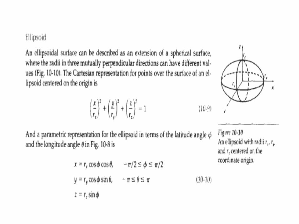
SPLINE REPRESENTATIONS

a spline is a flexible strip used to produce a smooth curve through a designated set of points. We can mathematically describe such a curve with a piecewise cubic polynomial function whose first and second derivatives are continuous across the various curve sections.

spline curve refers to any composite curve formed with polynomial sections satisfying specified continuity conditions at the boundary of the pieces. A spline surface can be described with two sets of orthogonal spline curves.

We specify a spline curve by giving a set of coordinate positions, called control points, which indicates the general shape of the curve.

Control Points are connected by two ways:-InterpolateWhen polynomial sections are fitted so that the curve passes througheach control point, the resulting curve is said to interpolate theset of control points. ApproximateOn the other hand, when the polynomials are fitted to the general control-point path without necessarily passing through any control point, the resulting curve is said to approximate the set of control points.

Convex Hull : The convex polygon boundary that encloses a set of control points is called the convex hull. One way to envision the shape of a convex hull is to imagine a rubber band stretched round the positions of the control points so that each control point is either on the perimeter of the hull or inside it.

Convex hulls provide a measure for the deviation of a curve or surface from the region bounding the control points.

A polyline connecting the sequence of control points for an approximation spline is usually displaved to remind a designer of the control-point ordering. This set of connected line segments is often referred to as the control graph of the curve.

•Zero-order parametric continuity, described as C0 continuity, means simplythat the curves meet. That is, the values of x, y, and z evaluated at u, for the firstcurve section are equal, respectively, to the values of x, y, and z evaluated at u,for the next curve section.

•First-order parametric continuity, refered to as C1 continuity, means that the first parametric derivatives (tangent lines) of the coordinate functions for two successive curve sections are equal at their joining point.

• Second-order parametric continuity, or C2 continuity, means that both the first and second parametric derivatives of the two curve sections are the same at the intersection.

Geometric Continuity Conditions In this case, we only require parametric derivatives of the two sections to be proportional to each other at their common boundaryinstead of equal to each other.

Zero-order geometric continuity, described as G0 continuity is the same as zero-order parametric continuity. That is, the two curves sections must have the same coordinate position at the boundary point.

First-order geometric continuity, or G' continuity, means that the parametric first derivatives are proportional at the intersection of two successive sections.

Second-order geometric continuity, or G2 continuity means that both the first and second parametric derivatives of the two curve sections are proportional at their boundary.

Spline Specifications

There are three equivalent methods for specifying a particular spline representation:(1) We can state the set of boundary conditions that are imposed on the spline (means u1 , u2); (2)State the matrix that characterizes the spline; (3) We can state the set of blending functions (or basis functions) that determine how specified geometric constraints on the curve are combined to calculate positions along the curve path.To illustrate these three equivalent specifications, suppose we have the following parametric cubic polynomial representation for the x coordinate along the path of a spline section :

These four boundary conditions are sufficient to determine thevalues of the four coefficients ax ,bx, cx and dx by x(0), x(1), x’(0), x’(1).

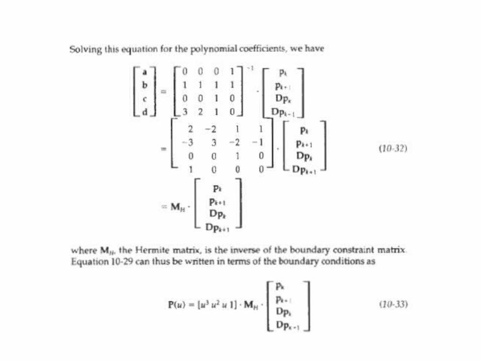
Where: Mgeom is a four-element column matrix containing the geometric constraint values (boundary conditions) on the spline; Mspline is the 4-by-4 matrix that transforms the geometric constraint values to the polynomial coefficients.

CUBIC SPLINE INTERPOLATION METHODS

Suppose we have n + 1 control points specified with Coordinates:

We can describe the parametric cubic polynomial that is to be fitted between each pair of control points with the following set of equations:

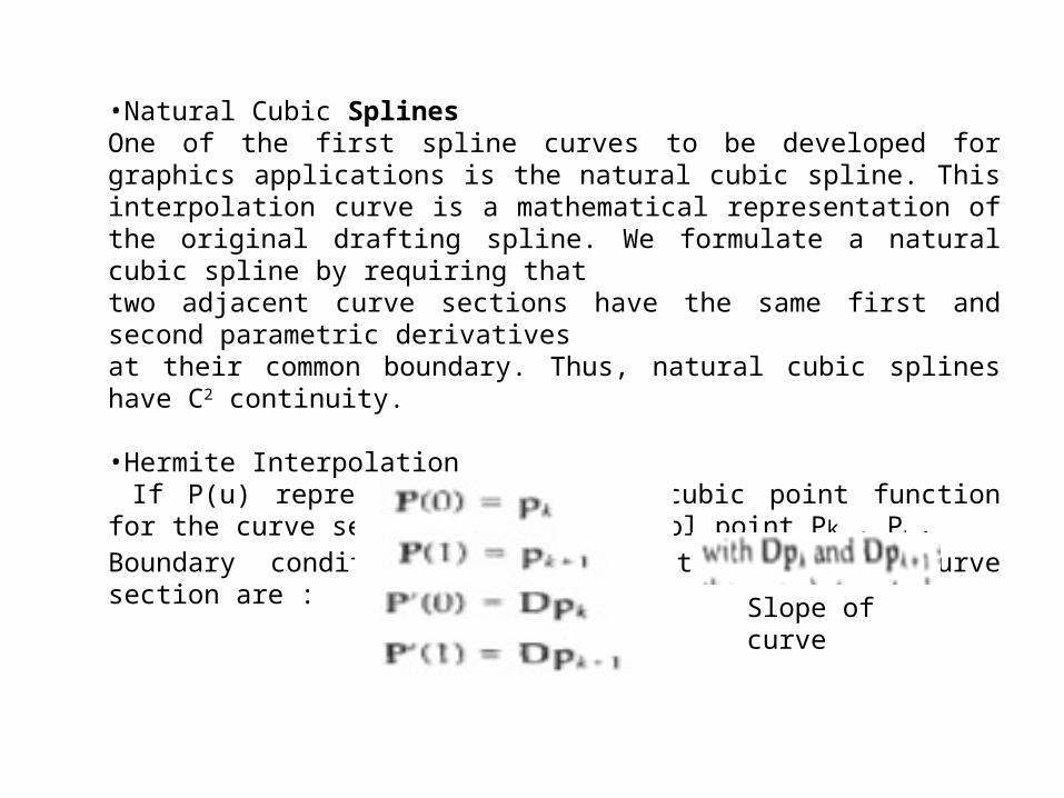
•Natural Cubic SplinesOne of the first spline curves to be developed for graphics applications is the natural cubic spline. This interpolation curve is a mathematical representation of the original drafting spline. We formulate a natural cubic spline by requiring thattwo adjacent curve sections have the same first and second parametric derivativesat their common boundary. Thus, natural cubic splines have C2 continuity.

•Hermite Interpolation If P(u) represent a parametric cubic point function for the curve section between control point Pk , Pk+1.

Boundary condition that define this Hermite curve section are :

Slope of curve

Cardinal splineFor a cardinal spline, the value for the slope at a control point is calculated from the coordinates of the two adjacent control points.

Parameter t is called the tension parameter since it controls how loosely or tightly the cardinal spline fits the input control points.

BEZIER CURVES AND SURFACESIn general, a Bezier curve section can be fitted to any number of control points. The number of control points to be approximated and their relative position determine the degree of the Bezier polynomial.

Properties of Bezier Curves •A very useful property of a Bezier curve is that it always passes through the first and last control points. That is, the boundary conditions at the two ends of the curve are

•Values of the parametric first derivatives of a Bezier curve at the endpoints can be calculated from control-point coordinates as

• The degree of the polynomial defining the curve segment is one less than the no. of defining polygon point.•The curve lies entirely within the convex Hull formed by four points. This follows from the properties of Bezier blending functions: They are all positive and their sum is

•Closed bezier curves are generated by specifying the first and last control points at the same time.

B-SPLINE CURVES AUD SURFACESThese are the most widely used class of approximating splines. B-splines havetwo advantages over Bezier splines: (1) The degree of a B-spline polynomial can be set independently of the

number of control points (with certain limitations). (2) B-splines allow local control over the shape of a spline curve or surface.

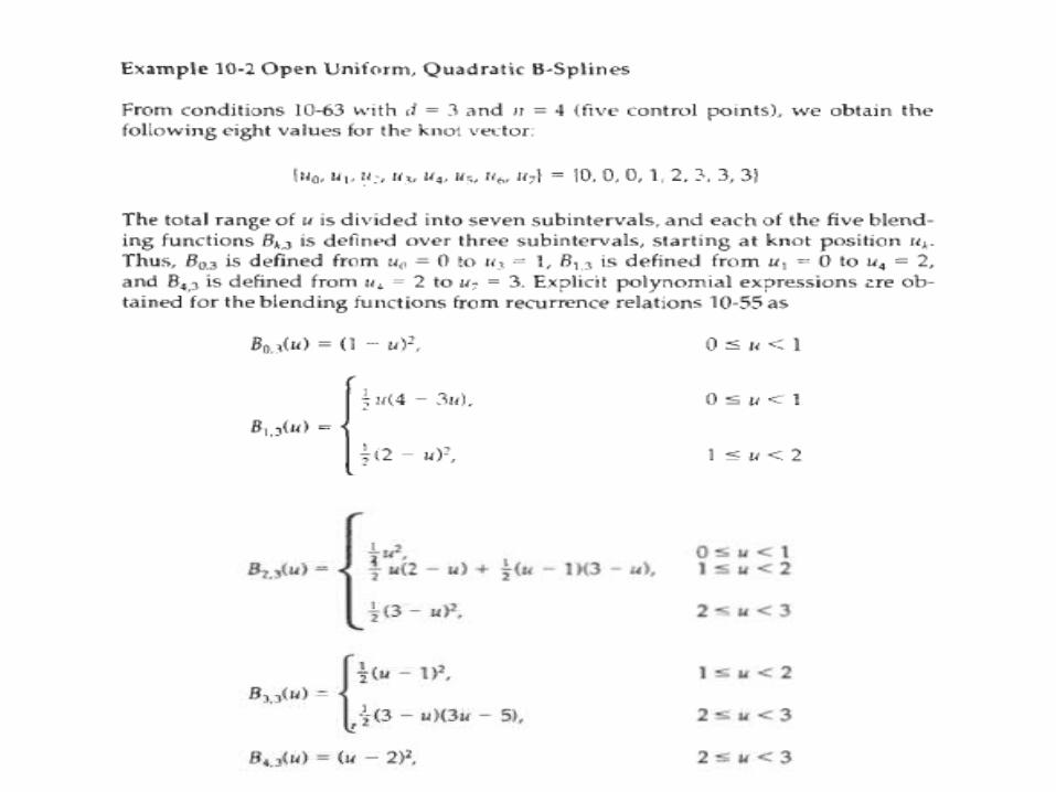
The Bspline blending functions B k,d are polynomials of degree d - 1,

If we set the value of d at 1, but then our "curve" is just a point plot of the control points.

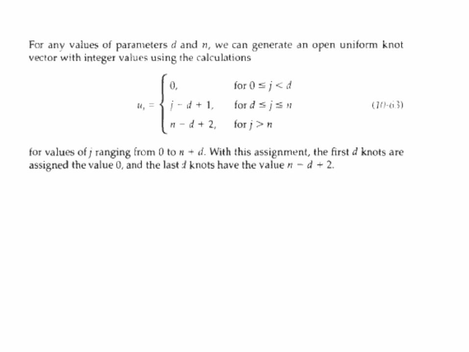
The selected set of subinterval endpoints u, is referred to as a knot vector. Wecan choose any values for the subinterval endpoints satisfying the relationu j<= u j+1 .Values for umin and umax then depend on the number of control points ,the value we choose for parameter d, and how we set up the subintervals (knot vector)

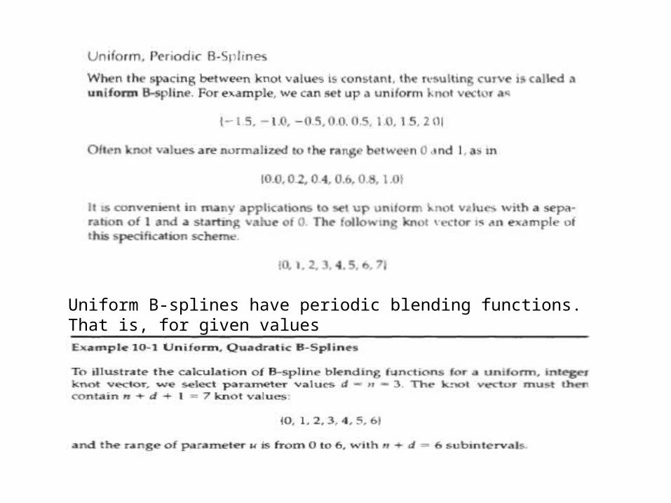
Uniform B-splines have periodic blending functions. That is, for given valuesof n and d, all blending functions have the same shape.

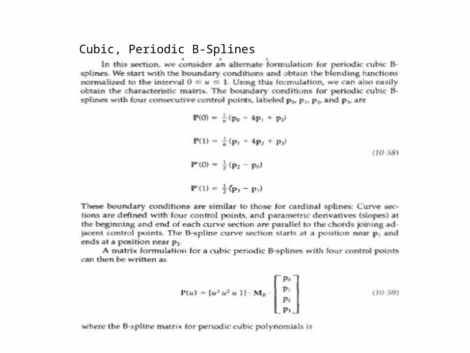
Cubic, Periodic B-Splines

HIDDEN LINES AND SURFACES

A main consideration in the generation of realistic graphics displays is identifying those parts of a scene that are visible from a chosen viewing position.The various algorithms are referred to as visible-surface detection methods. Sometimes these methods are also referred to as hidden-surface elimination methods.

CLASSIFICATION OF VISIBLE-SURFACE DETECTION ALGORITHMS

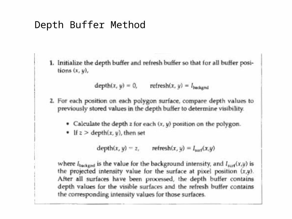
Depth Buffer Method

A-BUFFER METHOD

An extension of the ideas in the depth-buffer method is the A-buffer method. The A buffer method represents an antialiased, area-averaged, acc&dation-buffer method developed by Lucasfilm for implementation in the surface-rendering system called REYES. A drawback of the depth-buffer method is that it can only find one visiblesurface at each pixel position. In other words, it deals only with opaque surfacesand cannot accumulate intensity values for more than one surface, as is necessary if transparent surfaces are to be displayed . The A-buffer method expands the depth buffer so that each position in the buffer can reference a linked list of surfaces. Thus, more than one surface intensity can be taken into consideration at each pixel position, and object edges can be antialiased. Each position in the A-buffer has two fields:depth field - stores a positive or negative real number intensity field - stores surface-intensity information or a pointer value.

SCAN-LINE METHOD

This image space method for removing hidden surfaces is an extension of the scan-line algorithm for filling polygon interiors. Instead of filling just one surface, we now deal with multiple surfaces. As each scan line is processed, all polygon surfaces intersecting that line are examined to determine which are visible.Across each scan line, depth calculations are made for each overlapping surface to determine which is nearest to the view plane. When the visible surface has been determined, the intensity value for that position is entered into the refresh buffer.