arX

iv:1

711.

0634

5v1

[m

ath.

NT

] 1

6 N

ov 2

017

Quadratic rational functions with a rational periodic critical point

of period 3

Solomon Vishkautsan

with an appendix by Michael Stoll

Abstract

We provide a complete classification of possible graphs of rational preperiodic points ofquadratic rational functions defined over the rationals with a rational periodic critical pointof period 3, under two assumptions: that these functions have no periodic points of period atleast 5 and the conjectured enumeration of points on a certain genus 6 affine plane curve. Weshow that there are exactly six such possible graphs, and that rational functions satisfying theconditions above have at most eleven rational preperiodic points.

1 Introduction

In this article we continue the classification of preperiodicity graphs of quadratic rational functionsdefined over Q with a Q-rational periodic critical point that was begun in [CV17]. Our aim in thisarticle is to provide a complete classification of rational quadratic functions defined over Q with aQ-rational periodic critical point of period 3.

Let φ : P1 → P1 be a rational function, defined over some base field K. A point P ∈ P1 is calledperiodic for φ if there exists a positive integer n such that φn(P ) = P . The minimal such n is calledthe period of P . A point P ∈ P1 is called preperiodic for φ if there exists a nonnegative integer msuch that φm(P ) is periodic for φ.

One of the main motivations for this article is the following conjecture of Morton and Silverman[MS94].

Conjecture (Uniform Boundedness Conjecture). Let φ : PN → PN be a morphism of degree d ≥ 2defined over a number field K. Then the number of K-rational preperiodic points of φ is bounded

by a bound depending only on N and the degrees of K/Q and φ.

This powerful conjecture implies in particular Merel’s theorem of uniform boundedness of torsionsubgroups of the Mordell–Weil groups of rational points on elliptic curves (see [Sil07], Remark3.19), as well as the conjectured uniform boundedness of torsion subgroups of abelian varieties (see[Fak03]).

By Northcott’s theorem [Nor50], the set PrePer(φ,K) of K-rational preperiodic points of amorphism φ : PN → PN defined over a number field K, is finite. It can therefore be given a finitedirected graph structure, called the preperiodicity graph of φ, by drawing an arrow from P to φ(P )for each P ∈ PrePer(φ,K). The conjecture of Morton and Silverman implies in particular that

1

the number of possible preperiodicity graphs for such φ is finite and depends only on the constantsdeg(φ), [K : Q] and N . It is therefore natural to ask for the list of all possible preperiodicity graphsfor a given family of endomorphisms of PN .

The main example of a classification of preperiodicity graphs for rational functions is the clas-sification of preperiodicity graphs of quadratic polynomials over Q by Poonen [Poo98]. It relies onthe following conjecture.

Conjecture (Flynn, Poonen and Schaefer [FPS97]). Let φ be a quadratic polynomial defined over

Q. Then φ has no Q-rational periodic points of period greater than 3.

Evidence for this conjecture can be found in several articles, including [FPS97, Mor98, Sto08,HI13].

Theorem (Poonen). Assuming the Flynn, Poonen and Schaefer conjecture, there exist exactly 12possible preperiodicity graphs for quadratic polynomials defined over Q, and a quadratic polynomial

has at most nine Q-rational preperiodic points.

In the article [CV17], J.K. Canci and this author proposed a generalization of Poonen’s clas-sification of preperiodicity graphs of quadratic polynomials to the classification of preperiodicitygraphs of quadratic rational functions with a rational periodic critical point. Recall that a pointP ∈ P1 is called critical if φ′(P ) = 0 (if P or φ(P) are ∞ then we conjugate φ by an automorphismof P1, in order to move P and φ(P ) away from ∞). This is indeed a generalization of quadraticpolynomials since the latter are exactly quadratic rational functions with a rational fixed criticalpoint (up to conjugation by an automoprhism of P1). In [CV17], Canci and the author provideda full classification of preperiodicity graphs of quadratic rational functions defined over Q with aQ-rational periodic critical point of period 2, up to the following conjecture.

Conjecture 1. Let φ be a quadratic rational function defined over Q having a Q-rational periodic

critical point of period 2. Then φ has no Q-rational periodic points of period greater than 2.

Theorem. Assuming the conjecture above, there are exactly 13 possible preperiodicity graphs for

quadratic rational functions defined over Q with a Q-rational periodic critical point of period 2.Moreover, the number of Q-rational preperiodic points of such maps is at most 9.

In order to obtain a similar classification for quadratic rational functions with a Q-rationalperiodic critical point of period 3, we need to assume a similar conjecture to the conjecture ofFlynn, Poonen and Schaefer and Conjecture 1. First, let us define a critical n-cycle to be the set ofiterates of a periodic critical point of period n.

Conjecture 2. Let φ be a quadratic rational function defined over Q with a Q-rational critical 3-cycle. Then φ has no Q-rational periodic points of period greater than 2 lying outside of the critical

cycle.

As (slight) support for this conjecture, we show in section 4.3 that a rational function definedover Q with a Q-rational critical 3-cycle cannot have a Q-rational periodic point of period 3 or 4lying outside of the critical 3-cycle. For the classification of quadratic rational functions with acritical 3-cycle, we also need to assume the following conjecture.

2

Conjecture 3. The genus 6 affine plane curve defined by the affine equation

u5v2 + 2u4v3 − u4v2 − u4v + u3v4 − 4u3v2 + u3

+ u2v4 − 4u2v3 + 3u2v − 2uv3 + 4uv2 − u+ v2 − v = 0(1)

has Jacobian of Mordell–Weil rank exactly 2, and the Q-rational points on this curve are exactly

(−1, 0), (1, 1), (−1, 1), (0, 0), (0, 1), and (1, 0).

In the appendix to this article M. Stoll proves Conjecture 3, conditional on standard conjecturesincluding the BSD conjecture, by enumerating all rational points on the curve defined by Eq.(1)using the Chabauty–Coleman method.

Theorem 1. Assuming Conjectures 2 and 3, there are exactly six possible preperiodicity graphs for

quadratic rational functions defined over Q with a Q-rational critical 3-cycle. Moreover, the number

of preperiodic points of such maps is at most eleven.

The six possible preperiodicity graphs are listed below in Table 1, and for each graph we providean example of a rational function which realizes this graph (i.e., whose preperiodicity graph isisomorphic to the given graph). We say that a graph is realizable if there exists a rational functionthat realizes it.

The method by which we prove Theorem 1 is by showing (Section 4.2) that the graphs in Tables2, 3 and 4 below are inadmissible, i.e. that there exist no quadratic rational functions definedover Q with preperiodicity graphs containing isomorphic subgraphs. We prove in Section 3 thatthis is sufficient to prove Theorem 1. The way we prove inadmissibility of a given graph is byconstructing a dynamical modular curve whose Q-rational points correspond to conjugacy classes(under conjugation by automorphisms of P1) of rational functions defined over Q with a rationalcritical 3-cycle that admit the graph (i.e. whose preperiodicity graph contains an isomorphic copyof the graph). We then prove that the dynamical modular curve has no Q-rational points.

Acknowledgements. The author deeply thanks Michael Stoll and Maarten Derickx, withoutwhose help and advice this research would not have been completed. The author would also like tothank Benjamin Collas and Konstantin Jakob for many fruitful discussions during the preparationof this article. Finally the author would like to thank Fabrizio Catanese for his support and en-couragement. Research for this article has been supported by the Minerva Foundation and by ERCAdvanced Grant "TADMICAMT".

3

Table 1: Realizable quadratic rational functions with a Q-rat. periodic critical point of period 3ID φ(z) Preperiodicity graph

R3P01

(z − 1)2

•∞

•0

•1•2 ��cc

00

//

R3P12z2 − z − 1

2z2•0 •∞

•1•−1/2

•−1++

vv

UU66

rr

R3P2z2 + 5z − 6

z2•0 •∞

•1•−6

•6/5

•3

•2++

vv

UU66

rr

77♦♦♦♦♦♦♦♦♦♦

��

R3P35z2 − 7z + 2

5z2•0 •∞

•1•2/5

•2/7

•2

•1/3

++

vv

UU??⑧⑧⑧⑧⑧rr

$$❏❏❏

❏❏❏❏

❏❏❏❏

❏❏❏❏

❏

//

R3P43z2 − 5z + 2

3z2•0 •∞

•1•2/3

•2/5

•−2 •2 •1/3 •1/2

++

vv

UU66

rr

// ++jj oo

R3P55z2 − 11z + 6

5z2•0 •∞

•1•6/5

•6/11

•2/3 •2/5 •3 •−3/2

•6

•3/5

++

vv

UU66

rr

// **kk oo

''❖❖❖❖

❖❖❖❖

❖

77♦♦♦♦♦♦♦♦

4

We split the nine inadmissible graphs needed for the proof of Theorem 1 into three groups,according to the genus of the corresponding dynamical modular curve.

Table 2: Inadmissible graphs for quadratic rational functions with a critical 3-cycle with a modularcurve of genus 1

ID Preperiodicity graph genus

N3E1 •0 •∞

•1

• •

•

•

•

•++

vv

UU//

rr

77♦♦♦♦♦♦♦♦♦♦♦

��77♦♦♦♦♦♦♦♦♦♦♦

��1

N3E2 •0 •∞

•1•

•

•

•++

vv

UU66

rr

UU gg1

N3E3 •0 •∞

•1

• •

•

•

• •• •++

vv

UU//

rr

��❄❄❄

❄❄

??⑧⑧⑧⑧⑧

**jj// oo 1

Table 3: Inadmissible graphs for quadratic rational functions with a critical 3-cycle with a modularcurve of genus 2

ID Preperiodicity graph genus

N3M1 •0 •∞

•1

• •

•

•

•

• ++

vv

UU//

rr

��❄❄❄

❄❄

??⑧⑧⑧⑧⑧

��❄❄❄

❄❄

??⑧⑧⑧⑧⑧2

N3M2 •0 •∞

•1

• •

•

• •

•++

vv

UU//

rr

��❄❄❄

❄❄

??⑧⑧⑧⑧⑧

77♦♦♦♦♦♦♦♦♦♦♦

��2

N3M3 •0 •∞

•1•

• • •• •

• •

++

vv

UU66

rr

**jj// oo

//��

2

5

Table 4: Inadmissible graphs for quadratic rational functions with a critical 3-cycle with a modularcurve of genus > 2

ID Preperiodicity graph genus

N3H1 •0 •∞

•1•

•

•

•

•

•++

vv

UU66

rr

''❖❖❖❖

❖❖❖❖

❖❖❖

77♦♦♦♦♦♦♦♦♦♦♦

//��

3

N3H2 •0 •∞

•1•

•

• • • •

•

•

•

•

++

vv

UU66

rr

// **jj oo''❖❖❖❖

❖❖❖❖

❖❖❖

77♦♦♦♦♦♦♦♦♦♦♦

// 77♦♦♦♦♦♦♦♦♦♦♦

6

N3H3 •0 •∞

•1•

•

• • • •

•

• •

•

++

vv

UU66

rr

// **jj oo''❖❖❖❖

❖❖❖❖

❖❖❖

77♦♦♦♦♦♦♦♦♦♦♦

gg❖❖❖❖❖❖❖❖❖❖❖

ww♦♦♦♦♦♦♦♦♦♦♦

5

2 Preliminaries

2.1 Dynatomic polynomials

Let φ : P1 → P1 be a rational function. We write

φ = [F (X,Y ), G(X,Y )]

using homogeneous polynomials F and G. Let

φn(X,Y ) = [Fn(X,Y ), Gn(X,Y )]

be the n-th iterate of φ for n ≥ 1, and define

Φφ,n(X,Y ) = Y Fn(X,Y )−XGn(X,Y ).

We then define the n-th dynatomic polynomial by

Φ∗φ,n(X,Y ) =

∏

k|n(Φk,φ(X,Y ))µ(n/k),

6

where µ is the Moebius mu function (for the proof that Φ∗φ,n are actually polynomials, see [MS95,

Theorem 2.1]).It is easy to see that if P is a periodic point of period n then P is a root of Φ∗

φ,n. The converse isnot true however, and a root of Φ∗

φ,n can correspond to a periodic point of period strictly dividingn. For any n ≥ 1, we call the roots of Φ∗

φ,n periodic points of formal period n for φ.In the article we identify (by abuse of notation) the dynatomic polynomials Φ∗

φ,n(X,Y ) with

their dehomogenization Φ∗φ,n(z), where z = X

Y . By dehomogenizing, we ignore the possibility of ∞being a root of the dynatomic polynomials. This will not be a problem in what follows, however.

2.2 Linear equivalence of rational functions

We say that two rational functions φ1, φ2 : P1 → P1 are linearly equivalent if there exists anf ∈ PGL2 acting as a projective automorphism of P1 such that φ2 = φf1 = f−1φ1f .

Let φ1, φ2 be linearly equivalent. A point P is periodic of period n for φ1 if and only if f−1(P ) isperiodic of period n for φ2 (similarly for preperiodic points). When φ1, φ2 and f are all defined overthe same base field K, then it is clear that the preperiodicity graphs of φ1 and φ2 are isomorphic.Therefore when classifying realizable graphs of rational functions defined over Q we are actuallyinterested in the Q-rational conjugacy classes of quadratic rational functions rather than in theindividual maps.

2.3 Post-critically finite quadratic rational functions

A rational function φ : P1 → P1 is called post-critically finite (or PCF for short) if all of itscritical points are preperiodic. A rational function has exactly 2d− 2 critical points (counted withmultiplicity; see [Sil07], Section 1.2), and a quadratic rational function has exactly 2 distinct criticalpoints.

Lukas, Manes and Yap [LMY14] provided a complete classification of all quadratic post-criticallyrational functions over Q and their Q-conjugacy classes, as well as all possible preperiodicity graphsof these functions. In particular, they showed that a quadratic rational function defined over Q witha Q-rational critical 3-cycle is PCF if and only if both of its critical points lie in the same 3-cycle,and there is a unique conjugacy class of quadratic rational functions (over Q) with this property,realizing the graph R3P0 in Table 1.

3 Sufficiency of the nine inadmissibility graphs

Proposition 1. Assume Conjecture 2. Any quadratic rational function with a rational critical 3-cycle that does not realize one of the graphs in Table 1, must admit one of the graphs in Tables 2,

3 or 4.

Proof. We can arrange the graphs from Tables 1 through 4 in a Hasse diagram with respect to thepartial order of subgraph isomorphism:

7

R3P1

R3P2 R3P3 R3P4 N3E2

N3E1 N3H1 N3M2 N3M1 N3E3 R3P5 N3M3

N3H2 N3H3

❚❚❚❚❚❚❚❚❚❚❚

❄❄❄❄❄⑧⑧⑧⑧⑧

❥❥❥❥❥❥❥❥❥❥❥

❲❲❲❲❲❲❲❲❲❲❲❲❲❲❲❲❲

❖❖❖❖❖❖❖

❖❖❖❖❖❖❖

♦♦♦♦♦♦♦

♦♦♦♦♦♦♦

❣❣❣❣❣❣❣❣❣❣❣❣❣❣❣❣

♦♦♦♦♦♦♦

Due to the results of [LMY14] mentioned in Section 2.3, we can restrict ourselves to non-PCF(see Section 2.3) quadratic rational functions with a rational critical 3-cycle. Lemma 3.2 in [CV17]implies that starting from the critical cycle graph R3P1, one can obtain any realizable graph of anon-PCF rational function defined with a rational critical 3-cycle, by recursively adding verticesand arrows to the graph using either of the following two recursion steps:

1. Adding a periodic cycle. We add a new cycle C to the graph. For each vertex P in C weadd a vertex Q not in the cycle and an arrow Q → P .

2. Adding preimages to a non-periodic point. We add two vertices Q1, Q2 and arrowsQ1 → P,Q2 → P , where P is a vertex not lying in any cycle in the graph.

Now it is easy to check that from any graph in the Hasse diagram, by using one of the recursivesteps we either generate a graph that is already in the Hasse diagram, or contains (a subgraphisomorphic to) one of the nine graphs in Tables 2, 3 or 4.

4 Constructing dynamical modular curves from the graphs

4.1 Realizable graphs with a critical 3-cycle

4.1.1 R3P0

Note that graph R3P0 implies that we have two points in the 3-cycle which are critical. Since anyquadratic rational function has exactly two distinct critical points, this means any function admittingthe graph is post-critically finite (or PCF for short), i.e. all its critical points are preperiodic.

As mentioned in Section 2.3, Lukas, Manes and Yap proved in [LMY14] that there is onlyone possible preperiodicity graph for a PCF quadratic rational function with a critical three cycle,which is graph R3P0 in Table 1. Moreover, there is only one Q-conjugacy class of quadratic rationalfunctions that has this preperiodicity graph, with the following representative.

φ0(z) =1

(z − 1)2. (2)

4.1.2 R3P1

We can parametrize the non-PCF Q-conjugacy classes of quadratic rational functions with a rationalcritical 3-cycle using the following map.

a 7→ φa(z) =(a+ 1)z2 − az − 1

(a+ 1)z2, a 6= 0,−1,−2. (3)

8

For the special values a = 0,−2 we get representatives of the conjugacy class realizing the graphR3P0.

In fact, given any rational function φ defined over Q with a Q-rational critical 3-cycle, we canconjugate φ by an element of PGL2(Q) to move the periodic critical point P to 0, its image to ∞and φ2(P ) to 1. One can then check that we obtain a function φa for some a ∈ Q.

0 ∞

1− 1a+1

− 1a

**

uu

VV55

rr

Figure 1: Preperiodicity graph of φa

The preperiodicity graph of φa where a 6= 0,−1,−2 will contain the graph in Fig. 1; it is easyto check that the non-periodic preimages of 0 and 1 are − 1

a+1 and − 1a , respectively.

4.1.3 R3P2

We take the parametrization φa of R3P1 and consider a root b of the first dynatomic polynomial ofφa. Such a root must correspond to a fixed point of φa.

Φ∗a,1(b) := Φ∗

φa,1(b) = (1 + a)b3 + (−1− a)b2 + ab+ 1 = 0. (4)

We solve this equation for a.

a = −b3 − b2 + 1

b(b2 − b+ 1). (5)

We then substitute this into the expression for φa and get the following parametrization ofquadratic rational functions realizing R3P2.

b 7→ φb(z) =(b− 1)z2 + (b3 − b2 + 1)z − b3 + b2 − b

(b− 1)z2, (6)

where b cannot obtain the values 0, 1 in Q. We remark that φb degenerates also when b is a root ofb2 − b+ 1 = 0, but for this case b 6∈ Q. Moreover, the solutions to the equations

b3 − b2 + 1 = 0 and b3 − b2 + 2b− 1 = 0

determine a = 0 and a = 2, respectively, but these do not have Q-rational solutions either.Each map φb admits the graph in Fig. 2.

0 ∞

1− b3−b2+bb−1

b3−b2+bb3−b2+1

b2−b+1b2−2b+1

b**

uu

VV55

rr

77♦♦♦♦♦♦♦

��

Figure 2: Preperiodicity graph of φb

9

It is easy to check that

−b3 − b2 + b

b− 1,

b3 − b2 + b

b3 − b2 + 1and

b2 − b+ 1

(b− 1)2

are the non-periodic preimages of 0, 1 and b, respectively.

4.1.4 R3P3

We start again with φa parametrizing R3P1 (see Section 4.1.2). Recall that −1/(a + 1) is thenon-periodic preimage of 0. Let c be a preimage of −1/(a+ 1), i.e. φ(c) = − 1

a+1 . This implies thefollowing equation.

(a+ 2)c2 − ac− 1 = 0. (7)

We solve this equation for a.

a = −2 c2 − 1

c2 − c. (8)

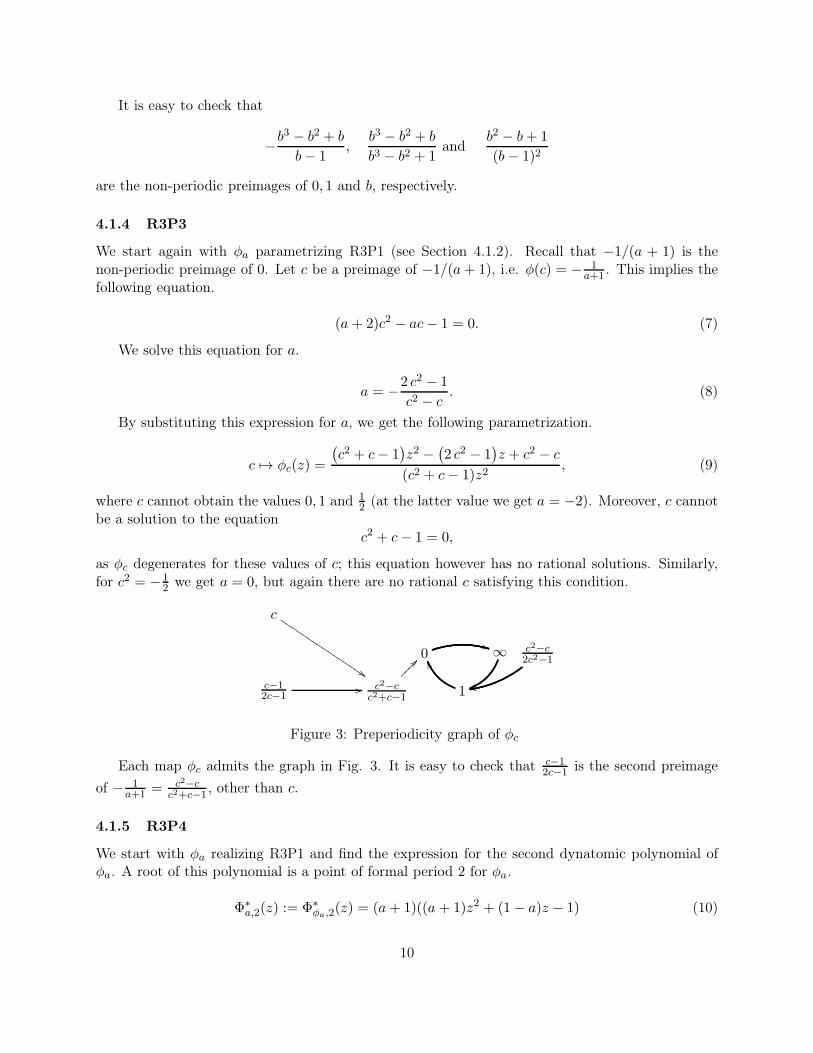
By substituting this expression for a, we get the following parametrization.

c 7→ φc(z) =

(

c2 + c− 1)

z2 −(

2 c2 − 1)

z + c2 − c

(c2 + c− 1)z2, (9)

where c cannot obtain the values 0, 1 and 12 (at the latter value we get a = −2). Moreover, c cannot

be a solution to the equationc2 + c− 1 = 0,

as φc degenerates for these values of c; this equation however has no rational solutions. Similarly,for c2 = −1

2 we get a = 0, but again there are no rational c satisfying this condition.

0 ∞

1c2−cc2+c−1

c2−c2c2−1

c

c−12c−1

**

uu

VV??⑧⑧⑧⑧rr

$$❏❏❏

❏❏❏❏

❏❏❏❏

❏❏❏❏

❏

//

Figure 3: Preperiodicity graph of φc

Each map φc admits the graph in Fig. 3. It is easy to check that c−12c−1 is the second preimage

of − 1a+1 = c2−c

c2+c−1, other than c.

4.1.5 R3P4

We start with φa realizing R3P1 and find the expression for the second dynatomic polynomial ofφa. A root of this polynomial is a point of formal period 2 for φa.

Φ∗a,2(z) := Φ∗

φa,2(z) = (a+ 1)((a + 1)z2 + (1− a)z − 1) (10)

10

A formal point of period 2 for φa is not of period 2 only if it is of period 1 and so a root ofthe first dynatomic polynomial Φ∗

a,1(z). One can find such points by computing the roots of theresultant of the first two dynatomic polynomials.

Res(Φ∗a,1(z),Φ

∗a,2(z)) = −(a+ 1)4(a2 + 2a+ 5)

We see that there are no Q-rational values of a which produce points of formal period 2 but ofactual period 1.

We see that any Q-rational periodic point d is of period 2 for φa if and only if it is a solution ofthe following equation.

(a+ 1)d2 + (1− a)d− 1 = 0. (11)

We solve this equation for a.

a = −d2 + d− 1

d2 − d. (12)

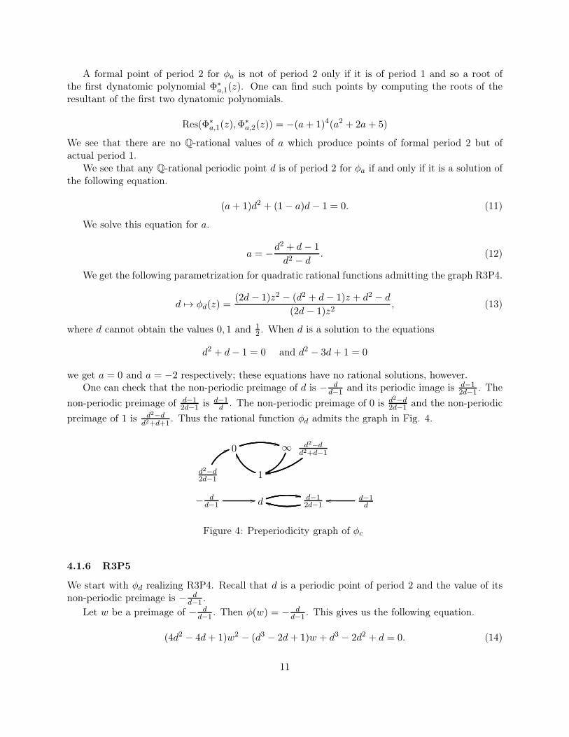
We get the following parametrization for quadratic rational functions admitting the graph R3P4.

d 7→ φd(z) =(2d − 1)z2 − (d2 + d− 1)z + d2 − d

(2d − 1)z2, (13)

where d cannot obtain the values 0, 1 and 12 . When d is a solution to the equations

d2 + d− 1 = 0 and d2 − 3d+ 1 = 0

we get a = 0 and a = −2 respectively; these equations have no rational solutions, however.One can check that the non-periodic preimage of d is − d

d−1 and its periodic image is d−12d−1 . The

non-periodic preimage of d−12d−1 is d−1

d . The non-periodic preimage of 0 is d2−d2d−1 and the non-periodic

preimage of 1 is d2−dd2+d+1

. Thus the rational function φd admits the graph in Fig. 4.

0 ∞

1d2−d2d−1

d2−dd2+d−1

− dd−1 d

d−12d−1

d−1d

**

uu

VV55

rr

// ,,jj oo

Figure 4: Preperiodicity graph of φc

4.1.6 R3P5

We start with φd realizing R3P4. Recall that d is a periodic point of period 2 and the value of itsnon-periodic preimage is − d

d−1 .

Let w be a preimage of − dd−1 . Then φ(w) = − d

d−1 . This gives us the following equation.

(4d2 − 4d+ 1)w2 − (d3 − 2d+ 1)w + d3 − 2d2 + d = 0. (14)

11

There are four solutions to this equation which correspond to degenerate maps φd, these are

(d,w) = (0, 0), (0, 1), (1, 0), (1

2, 1).

The discriminant of Eq. (14) with respect to w is:

∆ = d6 − 16d5 + 44d4 − 50d3 + 28d2 − 8d+ 1

= (d− 1)2(d4 − 14d3 + 15d2 − 6d+ 1)

Using the discriminant, we find that the affine plane curve defined by Eq. (14) is birational tothe affine plane curve defined by

y2 = x4 − 14x3 + 15x2 − 6x+ 1, (15)

where

x = d, y =2(4d2 − 4d+ 1)w − (d3 − 2d+ 1)

d− 1(16)

or

w =(d− 1)y + (d3 − 2d+ 1)

2(4d2 − 4d+ 1). (17)

We can simplify the curve defined by Eq. (15) further to get the elliptic curve

E : y2 + xy + y = x3 − x2. (18)

This elliptic curve is curve 53a1 in the Cremona database (see [Cre06]), it has rank 1 withtrivial torsion. We thus get infinitely many rational points on the curve, and thus infinitely manynon-linearly equivalent rational functions defined over Q admitting graph R3P5 (only finitely manyQ-rational points on E will be mapped to degenerate solutions of Eq. (14)).

4.2 Nonrealizable graphs with a critical 3-cycle

4.2.1 N3E1

We start with the graph R3P1 by taking the parametrization φa we defined in Section 4.1.2. Werecall that the general form of a quadratic rational function admitting R3P1 is

φa(z) =(a+ 1)z2 − az − 1

(a+ 1)z2, a 6= 0,−1,−2. (19)

We will show that the first dynatomic polynomial of φa cannot split over Q. This immediatelyimplies that a quadratic rational function with a rational critical three-cycle can have at most oneQ-rational fixed point.

The first dynatomic polynomial of φa is

Φ∗a,1(z) := Φ∗

φa,1(z) = (−a− 1)z3 + (a+ 1)z2 − az − 1. (20)

12

In R3P2 we determined that a root b of this polynomial must satisfy

a = −b3 − b2 + 1

b(b2 − b+ 1). (21)

A necessary and sufficient condition for the cubic polynomial Φ∗a,1 to split over Q is for it to

have a Q-rational root and for the discriminant to be a square in Q. The latter condition is definedby the following equation.

u2 = ∆(Φ∗a,1) = −3a4 − 16a3 − 50a2 − 60a− 23. (22)

Substituting (21) into (22) we obtain

v2 = (b− 1)(b3 + b2 − b+ 3), (23)

where

v =b2(b2 − b+ 1)2u

2b3 − 4b2 + 2b− 1.

The affine plane curve C defined by (23) is of genus 1. We denote by C its projective closure inP2[X:Y :Z] where b = X/Z and v = Y/Z. The curve C contains (at least) the following two Q-rational

points:[0 : 1 : 0], [1 : 0 : 1].

It is birational to the elliptic curve with Cremona reference 19a3 with minimal model

E : y2 + y = x3 + x2 + x.

Remark 1. It is interesting to note that the elliptic curve with Cremona reference 19a3 appearsseveral times in the classification of preperiodicity graphs of rational functions with a rationalcritical cycle. For example, in [CV17] it is proven that it is birational to two modular curves ofquite distinct graphs with critical 2-cycles (denoted there by N2E2 and N2E3), and it appears againbelow in Section 4.3.2. Similarly, the elliptic curve with Cremona reference 17a4 appears both forN3E3 below (see Section 4.2.3 below) and for the proof of Proposition 4.3 in [CV17]. The ellipticcurve with Cremona reference 11a3 appears for N3E2 below (see Section 4.2.2 below) and for thegraph N2E1 in [CV17].

The birational map ψ : C → E is given by

ψ([X : Y : Z]) = [2Z2 − 2XZ,X2 − 2XZ + Y Z + Z2,−2X2 + 4XZ − 2Z2].

The rational points in the locus of indeterminacy of ψ are exactly the two points we have alreadydiscovered on C. The elliptic curve E has Mordell–Weil group of rank 0 and torsion subgroupisomorphic to Z/3Z. It therefore contains only three rational points, which are

[0 : 0 : 1], [0 : 1 : 0], [0 : −1 : 1].

The preimages of these points under the birational map ψ, together with ψ’s locus of indeterminacygive us the full set of points on C, and it turns out that the two points we found on C are the onlyrational points on it. Neither of these points corresponds to a non-degenerate quadratic rationalfunction φb.

As an aside, we prove the following.

13

Proposition 2. There exists a unique conjugacy class of quadratic rational functions with a critical

3-cycle whose first dynatomic polynomial has a square Q-rational discriminant.

Proof. The affine plane curve C1 described by Eq.(22) has genus 1, and it is birational to the ellipticcurve with Cremona reference 19a1 with the following minimal model.

E1 : y2 + y = x3 + x2 − 9x− 15. (24)

We consider the projective closure C1 of C1 in P2[X:Y :Z] where a = X

Z and u = YZ . The birational

map ψ : C1 → E1 is given by

ψ = [1491X3 + 4176X2Z − 133XY Z + 3821XZ2 − 114Y Z2 + 1146Z3,

533X3 + 2839X2Z + 171XY Z + 3891XZ2 + 95Y Z2 + 1565Z3,

− 686X3 − 1764X2Z − 1512XZ2 − 432Z3].

The elliptic curve E1 has Mordell–Weil rank 0, and torsion subgroup isomorphic to Z/3Z. Thethree rational points on E are

[0 : 1 : 0], [5 : 9 : 1], [5 : −10 : 1]. (25)

The only rational preimages of these points under ψ, together with ψ’s points of indeterminacyare the four points

[−6/7 : −19/49 : 1], [−6/7 : 19/49 : 1], [0 : 1 : 0], [−1 : 0 : 1]. (26)

These are therefore the only rational points on the curve C1. The third point is at infinity andis therefore a "cusp" (a point added to the dynamical modular curve to obtain a projective curve),while the fourth point corresponds to the case a = −1 for which φa is a degenerate map.

It remains to check the case a = −67 . For this map we get the following first dynatomic

polynomial

Φ∗− 6

7,1(z) = −

1

7(z3 − z2 − 6z + 7) (27)

whose discriminant 3612401 = (1949 )

2 is a square in Q as expected. However, this polynomial is irreducibleand therefore φ− 6

7

has no Q-rational fixed points.

4.2.2 N3E2

We start with the parametrization φa of R3P1. Recall that the non-periodic preimage of 1 is − 1a .

Assume that − 1a has a preimage t, i.e. φ(t) = − 1

a . This implies the following equation.

a2t2 − a2t+ 2at2 + t2 − a = 0. (28)

The curve C2 described by this equation is of genus 1. We take the projective closure C2 of C2

in P2[X:Y :Z] where a = X

Z and t = YZ . C2 contains (at least) the following 4 rational points:

[0 : 1 : 0], [0 : 0 : 1], [1 : 0 : 0], [−1 : 1 : 1]. (29)

14

The affine plane curve C2 is birational to the elliptic curve E with reference 11a3 in the Cremonadatabase. Its minimal model is given by

E : y2 + y = x3 − x2. (30)

This elliptic curve has Mordell–Weil rank 0 and a torsion subgroup isomorphic to Z/5Z and 5rational points:

[0 : 1 : 0], [0 : 0 : 1], [0 : −1 : 1], [1 : 0 : 1], [1 : −1 : 1]. (31)

The birational map ψ : C2 → E is defined by

ψ = [XY 3 −XY 2Z + Y 3Z − Y Z3,

−XY 2Z + Y 3Z +XY Z2 − 2Y 2Z2 + Z4,

− Y 3Z].

The preimages of the rational points under ψ together with ψ’s points of indeterminacy ([1 :0 : 0], [0 : 1 : 0]) are the four points of C2 we have already discovered. Therefore these are all therational points on C2.

None of these points corresponds to a non-degenerate map φa, therefore graph N3E2 is non-realizable.

4.2.3 N3E3

We start the quadratic rational function φc parametrizing R3P3 (note that we could also havestarted with R3P4).

φc(z) =

(

c2 + c− 1)

z2 −(

2 c2 − 1)

z + c2 − c

(c2 + c− 1)z2, c 6= 0, 1,

1

2. (32)

We consider the second dynatomic polynomial for φc.

Φ∗c,2(z) := Φ∗

φc,2(z) =(c4 + 2c3 − c2 − 2c+ 1)z2

+ (−3c4 − 2c3 + 5c2 − 1)z + c4 − 2c2 + c

This polynomial is divisible by c2 + c− 1; since the map φc degenerates for the two values of cwhich are its roots, we can divide by it to get

c2z2 − 3c2z + c2 + cz2 + cz − c− z2 + z = 0. (33)

This equation describes a genus 1 affine plane curve which we will denote by C3, and its projectiveclosure in P2

[X:Y :Z] by C3, where c = XZ and z = Y

Z . The curve C3 contains (at least) the following6 points:

[1 : 1 : 1], [0 : 1 : 0], [0 : 0 : 1], [0 : 1 : 1], [1 : 0 : 0], [1 : 0 : 1]. (34)

This curve is birational to the elliptic curve

15

E : y2 + xy + y = x3 − x2 − x (35)

with Cremona reference 17a4. This curve has Mordell-Weil rank 0 and torsion subgroup isomorphicto Z/4Z, and thus contains exactly four Q-rational points which are

[0 : 0 : 1], [0 : 1 : 0], [0 : −1 : 1], [1 : −1 : 1].

The map ψ from C3 to E is defined by

ψ = [XY 3 − 4XY 2Z + 4XY Z2 + Y 2Z2 −XZ3 − 2Y Z3 + Z4,

XY 2Z − 3XY Z2 +XZ3 + Y Z3 − Z4,

− Y 3Z + 3Y 2Z2 − 3Y Z3 + Z4].

The points of indeterminacy of ψ are [0 : 1 : 1], [0 : 1 : 0], [1 : 0 : 0].The preimages of the four rational points of E under ψ together with ψ’s points of indeterminacy

give us all the rational points of C3, and these are exactly the six points that we have alreadydiscovered, none of which correspond to non-degenerate quadratic rational functions.

4.2.4 N3M1

We start with the parametrization φc of the graph R3P3. Recall that c is a preperiodic point whoseimage under φc is the non-periodic preimage of 0. Let w be a preimage of c under φc, i.e. φ(w) = c.This implies

− c3w2 − 2c2w + 2cw2 + c2 −w2 − c+ w = 0 (36)

This equation describes an affine plane curve that we denote by C4, and we denote its projectiveclosure in P2

[X:Y :Z] by C4, where c = XZ and w = Y

Z . This curve is of genus 2 and contains (at least)the following five points.

[0 : 1 : 0], [0 : 0 : 1], [0 : 1 : 1], [1 : 0 : 0], [1 : 0 : 1]. (37)

The curve C4 is birational to the hyperelliptic curve given by

H : y2 = x6 − 2x5 + 3x4 − 4x3 − x2 + 2x+ 1. (38)

The birational map ψ : C4 → H is defined by

ψ = [−XZ + Z2, 2X3Y Z2 + 2X2Z4 − 4XY Z4 + 2Y Z5 − Z6,−XZ].

The latter curve H contains the following points (in weighted homogeneous coordinates):

[1 : −1 : 0], [1 : 1 : 0], [0 : −1 : 1], [0 : 1 : 1], [1 : 0 : 1]. (39)

The hyperelliptic curve has Jacobian with torsion subgroup isomorphic to Z/15Z, and a rankbound computation in Magma [BCP97] tells us the Jacobian has Mordell–Weil rank 0.

The curve H has good reduction at 3, and therefore the Mordell-Weil group of the JacobianJ(Q) of H injects into J(F3). Therefore all the maps in the following commutative diagram areinjective.

16

H(Q) J(Q)

H(F3) J(F3)

However, one can easily check that the only rational points in H(F3) are the reductions (mod 3)of the five points in H(Q) we have already discovered. Therefore these five points are the only Q-rational points on H.

Using ψ we pull back these five points to C4, and together with the indeterminacy points of ψ(these are [0 : 1 : 0], [1 : 0 : 0]) we find that the only rational points on C are the five points wefound before. None of these points correspond to non-degenerate quadratic rational functions.

4.2.5 N3M2

We start with the parametrization φc of the graph R3P3, and consider a root w of its first dynatomicpolynomial. Such a root must correspond to a fixed point of φc.

Φ∗c,1(w) := Φ∗

φc,1(w) =(−c2 − c+ 1)w3 + (c2 + c− 1)w2

+ (−2c2 + 1)w + c2 − c = 0.

We denote by C5 the affine plane curve defined by this equation, and by C5 its projective closurein P2

[X:Y :Z], where c = XZ and w = Y

Z . This is a curve of genus 2 and contains (at least) the followingfour rational points

[0 : 1 : 0], [0 : 0 : 1], [1 : 0 : 0], [1 : 0 : 1]. (40)

This curve is birational to the following hyperelliptic curve

H5 : y2 = x6 − 2x5 + 5x4 − 6x3 + 10x2 − 8x+ 5. (41)

The birational map ψ : C5 → H5 is defined by

ψ = [− Y Z + Z2,

2XY 3Z2 − 2XY 2Z3 + Y 3Z3 + 4XY Z4 − Y 2Z4 − 2XZ5 + Z6,

− Y Z].

One can use Magma to check that the Jacobian J of H5 has Mordell–Weil torsion subgroupisomorphic to Z/5Z and rank 0. The curve H5 contains (at least) the following two rational points(in weighted homogeneous coordinates).

[1 : −1 : 0], [1 : 1 : 0]. (42)

The Jacobian J contains (at least) the following rational points in Mumford representation:

(1, 0, 0), (1, x3 − x2, 2), (1,−x3 + x2, 2), (x2 − x+ 1, x− 1, 2), (x2 − x+ 1,−x+ 1, 2).

17

We denote by P+ = [1 : 1 : 0] and P− = [1 : −1 : 0], the two points at infinity. Using thisnotation we get the following divisor representations on H:

(1, 0, 0) ≡ identity,

(1, x3 − x2, 2) ≡ P+ − P−,

(1,−x3 + x2, 2) ≡ P− − P+,

(x2 − x+ 1, x− 1, 2) ≡ [α : −α : 1] + [α : −α : 1]− P+ − P−,

(x2 − x+ 1,−x+ 1, 2) ≡ [α : α : 1] + [α : α : 1]− P+ − P−,

where α = 12 +

√−32 . The only rational points appearing in these representations are the two we

already found, and therefore they are the only rational points on H5.Pulling back the two rational points of H5 under ψ and adding its indeterminacy points, we

find all rational points on C5, and these are exactly the four points we found before. None of thesepoints correspond to non-degenerate quadratic rational functions.

4.2.6 N3M3

We start with R3P4 and consider a root w of first dynatomic polynomial of φd (note that we canalso start with R3P2 and look at the second dynatomic polynomial of φb). Such a root correspondsto a fixed point of φd.

Φ∗d,1(w) := Φ∗

d,1(w) =(−2d+ 1)w3 + (2d− 1)w2 + (−d2 − d+ 1)w + d2 − d = 0

The affine plane curve C6 described by this equation is of genus 2. We denote its projectiveclosure in P2

[X:Y :Z] by C6, where d = XZ and w = Y

Z . The curve C6 contains (at least) the followingfive rational points

[0 : 1 : 0], [0 : 0 : 1], [1 : 2 : 2], [1 : 0 : 0], [1 : 0 : 1], (43)

and is birational to the hyperelliptic curve

H : y2 = x6 + 2x5 + 5x4 + 8x3 + 12x2 + 8x+ 4 (44)

under the map ψ : C6 → H defined by

ψ = [Z, 2Y 3 + 2XY Z − 2Y 2Z − 2XZ2 + Y Z2 + Z3,−Y ].

Using Magma one can compute that the hyperelliptic curve H has Jacobian with Mordell–Weiltorsion subgroup isomorphic to Z/2Z and rank bounded by 1. The curve H contains (at least) thefollowing six rational points

[1 : −1 : 0], [1 : 1 : 0], [−1 : −2 : 1], [−1 : 2 : 1], [0 : −2 : 1], [0 : 2 : 1]. (45)

We denote by P+ = [1 : 1 : 0] and P− = [1 : −1 : 0], the two points at infinity. One can checkthat P+ − P− is of infinite order, and therefore the Mordell-Weil rank of the Jacobian is exactly1. Using the Chabauty–Coleman/ Mordell–Weil sieving algorithm (see Bruin and Stoll [BS10])implementation in Magma, we determine that the six points we have already found are the onlyrational points on H. Pulling them back to C6, we find (together with the indeterminacy point[1 : 0 : 0] of ψ) that the only rational points on C6 are the five points we have already found. Noneof these correspond to non-degenerate quadratic rational functions.

18

4.2.7 N3H1

We start with R3P2. Recall that

φb(z) =(b− 1)z2 + (b3 − b2 + 1)z − b3 + b2 − b

(b− 1)z2, b 6= 0, 1 (46)

is a parametrization of R3P2, where b is the fixed point and b2−b+1(b−1)2

is its non-periodic preimage.

Assume w is a preimage of b2−b+1(b−1)2

, i.e. φb(w) =b2−b+1(b−1)2

. This implies

bw2 − (b4 − 2b3 + b2 + b− 1)w + b4 − 2b3 + 2b2 − b = 0. (47)

We denote by C7 the affine plane curve defined by this equation, and by C7 its projective closurein P2

[X:Y :Z], where b = XZ and w = Y

Z . The curve C7 has genus 3, and contains (at least) the followingrational points

[0 : 1 : 0], [0 : 0 : 1], [1 : 0 : 0], [1 : 0 : 1]. (48)

The curve C7 is birational to the following hyperelliptic curve

H : y2 = 4x7 − 11x6 + 14x5 − 7x4 − 2x3 + 6x2 − 4x+ 1. (49)

The birational map ψ : C7 → H is defined by:

ψ = [−Z,X4 − 2X3Z +X2Z2 − 2XY Z2 +XZ3 − Z4,X − Z].

The curve H contains (at least) the following five points:

[1 : 0 : 0], [0 : −1 : 1], [0 : 1 : 1], [1 : −1 : 1], [1 : 1 : 1]. (50)

Using Magma, one can compute that the curve H has Jacobian J with Mordell–Weil rank 0,and torsion subgroup of order bounded by 72, and a two-torsion subgroup isomorphic to Z/2Z.

Let P = [0 : −1 : 1], Q = [1 : −1 : 1]. The divisor class [P-Q] has order 36 in the Jacobian.This means that if the torsion subgroup has order 72 then it is isomorphic to either Z/72Z orZ/36Z×Z/2Z. However, the second option is ruled out by the structure of the two-torsion subgroup.Therefore the only two options for the torsion subgroup are either Z/72Z or Z/36Z.

The image of [P −Q] under the map J(Q) → J(F5) ∼= Z/72Z × Z/2Z is not divisible by 2. Infact, under the identification of J(F5) with Z/72Z×Z/2Z, [P −Q] is mapped to the element (38, 1),which is not divisible by 2.

Therefore the Mordell–Weil group is isomorphic to Z/36Z, and is generated by [P − Q]. Thecurve H has good reduction at 5 so that all the maps in the following commutative diagram areinjective.

H(Q) J(Q)

H(F5) J(F5)

ı

19

There are six points in H(F5) (given in weighted homogeneous coordinates):

[1 : 0 : 0], [0 : 1 : 1], [0 : 4 : 1], [1 : 1 : 1], [1 : 4 : 1], [2 : 0 : 1]. (51)

Of these points, only the five points [1 : 0 : 0], [0 : 1 : 1], [0 : 4 : 1], [1 : 1 : 1], [1 : 4 : 1] map to theimage of the map ı in the diagram, and these exactly correspond to the five points we know on H.Since the map H(Q) → H(F5) is injective, this proves that these are the only rational points on H.

Combining the preimages of ψ together with its locus of indeterminacy, we find all rationalpoints on C7, and these are exactly the four points we already discovered. None of these four pointscorrespond to φb admitting the graph N3H1.

4.2.8 N3H2

For the proof that the graph N3H2 is non-admissible (up to standard conjectures) see the appendixby M. Stoll.

4.2.9 N3H3

We start with R3P5. Recall that graph R3P4 had the parametrization

φd(z) =(2d− 1)z2 − (d2 + d− 1)z + d2 − d

(2d− 1)z2, d 6= 0, 1,

1

2, (52)

where d is a periodic point of (formal) period 2, and the graph R3P5 was represented by the followingadditional condition.

(4d2 − 4d+ 1)w2 − (d3 − 2d+ 1)w + d3 − 2d2 + d = 0. (53)

The point w was such that φ2(w) = d and φ(w) is non-periodic. The second periodic point ofperiod 2 is d−1

2d−1 and its non-periodic preimage is d−1d . Let u be a rational preimage of d−1

d , i.e.

φ(u) = d−1d . This implies

(2d− 1)u2 − (d3 + d2 − d)u+ d3 − d2 = 0. (54)

Together with Eq. (53), we get the following affine space curve parametrizing the graph N3H3:

C1 :

{

(4d2 − 4d+ 1)w2 − (d3 − 2d+ 1)w + d3 − 2d2 + d = 0

(2d− 1)u2 − (d3 + d2 − d)u+ d3 − d2 = 0.(55)

Using the discriminant (with respect to u) we can bring the second equation to the form

v2 = d4 + 2d3 − 9d2 + 10d− 3 (56)

where

v =(4d− 2)u− (d3 + d2 − d)

d, (57)

and we have already seen in Section 4.1.6 that Eq. (54) can be transformed in a similar way to

y2 = d4 − 14d3 + 15d2 − 6d+ 1. (58)

20

Thus the curve C1 is birational to a curve C2 in A3(d,y,v) defined by

C2 :

{

y2 = d4 − 14d3 + 15d2 − 6d+ 1

v2 = d4 + 2d3 − 9d2 + 10d − 3. (59)

The curve C2 is of genus 5, and is a double-cover of the following curve:

H1 : s2 = (d4 − 14d3 + 15d2 − 6d+ 1)(d4 + 2d3 − 9d2 + 10d− 3). (60)

The curve H1 has genus 3, and its equation can be simplified to the following model:

H2 : y2 = −3x8 + 4x7 − 2x6 − 16x5 + 11x4 + 16x3 − 2x2 − 4x− 3. (61)

This curve has automorphism group Z/2Z × Z/2Z. When quotienting the curve by the auto-morphism [Z : −Y : −X], we get the following curve:

H3 : y2 = −3x6 + 4x5 − 26x4 + 12x3 − 55x2 − 16x+ 4. (62)

This genus 2 hyperelliptic curve contains (at least) the following two points:

P1 = [0 : −2 : 1], P2 = [0 : 2 : 1]. (63)

Using Magma, one can compute that H3 has Jacobian with Mordell–Weil rank bounded by1, and torsion subgroup isomorphic to Z/2Z. The divisor class [P1 − P2] has infinite order in theJacobian, and therefore generates a finite index subgroup of the Mordell–Weil group. We can usethe implementation of the Chabauty–Coleman/Mordell–Weil sieving algorithm (cf. Bruin and Stoll[BS10]) in Magma, and find that the only rational points on the curve are the two points we hadalready discovered.

We pull these two points all the way back C1 to find the complete set of rational points on thelatter curve (not including 4 points at infinity):

(1/2, 1, 1), (1, 0, 0), (0, 0, 0), (1, 1, 0), (0, 0, 1).

None of these points have a d value corresponding to a quadratic rational function φd realizingN3H3.

4.3 Support for Conjecture 1

4.3.1 Extra 3-cycle

We compute the 3-rd dynatomic polynomial of φa.

Φ∗a,3(z) := Φ∗

φa,3(z) =(a5 + 5a4 + 10a3 + 10a2 + 5a+ 1)z5

+ (−2a5 − 7a4 − 9a3 − 4a2 + a+ 1)z4

+ (a5 − 7a3 − 13a2 − 10a− 3)z3

+ (2a4 + 5a3 + 4a2 + a)z2

+ (a3 + 3a2 + 3a+ 1)z

21

We divide the dynatomic polynomial by the factor (a+1)z(z− 1) to get the irreducible polynomial

P3 := a3z3 − a3z2 + 3a2z3 − 2a2z + 3az3 + 2az2 − 2az − a+ z3 + 2z2 − z − 1

The curve C3 defined by the equation P3 = 0 contains the four points

[0 : 1 : 0], [−1 : 0 : 1], [1 : 0 : 0], [−1 : 1 : 1].

Furthermore, C3 is birational to the genus 2 hyperelliptic curve defined by

H3 : y2 = x6 − 4x5 + 6x4 − 2x3 + x2 − 2x+ 1

Using Magma, we can check that H3 has Jacobian of Mordell–Weil rank 0. The curve H3 hasgood reduction modulo 3, and its reduction has Jacobian isomoprphic to the group Z/19Z. Thismeans that Mordell–Weil group (of the Jacobian) of H3 is either trivial or isomorphic to Z/19Z.However, one can check that the element on the Jacobian defined by the difference of the two pointsat infinity [1 : −1 : 0] − [1 : 1 : 0] has order 19 and therefore the Jacobian of H3 is isomorphic toZ/19Z.

We get the following commutative diagram where all the maps are injective.

H3(Q) J(Q)

H3(F3) J(F3)

We check that

H3(F3) = {[1 : −1 : 0], [1 : 1 : 0], [0 : −1 : 1], [0 : 1 : 1], [1 : −1 : 1], [1 : 1 : 1]}.

All of these points are reductions of points from H3(Q), and this implies that the Q-rational pointson H3 are exactly the six points

[1 : −1 : 0], [1 : 1 : 0], [0 : −1 : 1], [0 : 1 : 1], [1 : −1 : 1], [1 : 1 : 1].

We pull these points back to C3, to find that the only rational points on C3 are the four pointswe already discovered. None of which correspond to non-degenerate maps φa.

4.3.2 Extra 4-cycle

We compute the 4th dynatomic polynomial of φa, and divide by a factor of (a + 1)4, to get thefollowing polynomial.

22

P4(a, t) :=(a6 + 6a5 + 15a4 + 20a3 + 15a2 + 6a+ 1)z12

+ (−2a7 − 19a6 − 64a5 − 107a4 − 98a3 − 49a2 − 12a− 1)z11

+ (a8 + 16a7 + 77a6 + 152a5 + 128a4 + 16a3 − 46a2 − 30a− 6)z10

+ (−3a8 − 27a7 − 58a6 + 38a5 + 248a4 + 304a3 + 165a2 + 41a+ 4)z9

+ (3a8 + 8a7 − 61a6 − 239a5 − 240a4 − 8a3 + 111a2 + 59a+ 9)z8

+ (−a8 + 11a7 + 64a6 + 10a5 − 251a4 − 317a3 − 126a2 − 8a+ 2)z7

+ (−6a7 + 12a6 + 128a5 + 133a4 − 94a3 − 153a2 − 48a− 1)z6

+ (−16a6 − 5a5 + 130a4 + 156a3 − a2 − 42a− 8)z5

+ (−25a5 − 26a4 + 78a3 + 94a2 + 12a− 7)z4

+ (−25a4 − 31a3 + 26a2 + 33a+ 5)z3

+ (−16a3 − 20a2 + 2a+ 5)z2

+ (−6a2 − 7a− 1)z − a− 1.

The equation P4 = 0 describes an affine plane curve of genus 12 which we denote by C4. Wefollow the trace map method described in [Mor98]: Let

tr4(z) = z + φ(z) + φ2(z) + φ3(z).

The image of the curve C4 under the map Ψ : (a, z) 7→ (a, tr4(z)) is birational to the quotient curveC4/ 〈σ〉, where σ is the automorphism of C4 defined by (a, z) 7→ (a, φ(z)). When φ is a polynomial,the image of Ψ can be calculated by taking the resultant of Φ∗

a,4(z) and t− tr4(z) with respect toz. However, in our case t− tr4(z) is not a polynomial, since tr4(z) is a rational function in z. Wefix this by clearing out the denominator of tr4(z); we denote the numerator of tr4 by A and thedenominator by B.

We compute the resultant Res(P4, Bt−A) and find the following irreducible factor.

P4(a, t) = a7t− 2 a6t2 + a5t3 − a7 + 13 a6t− 17 a5t2 + 5 a4t3−

7 a6 + 53 a5t− 47 a4t2 + 10 a3t3 − 6 a5 + 80 a4t−

60 a3t2 + 10 a2t3 + 43 a4 + 42 a3t− 38 a2t2 + 5 at3+

95 a3 − 10 a2t− 11 at2 + t3 + 89 a2 − 19 at− t2 + 42 a− 6 t+ 9

The degree 8 curve defined by P4 = 0 is of genus 1. It is birational to the elliptic curve withCremona reference 19a3 (this curve has already been encountered as being birational to the modularcurve of N3E1, see the remark in Section 4.2.1), and has the following minimal model

y2 + y = x3 + x2 + x.

Its Mordell–Weil group is isomorphic to Z/3Z and therefore there are exactly three rationalpoints on this elliptic curve. These are

[0 : 0 : 1], [0 : 1 : 0], [0 : −1 : 1].

23

Pulling these points back to the curve C4/ 〈σ〉, we find all rational points on C4/ 〈σ〉 to be

[0 : 1 : 0], [1 : 0 : 0], [1 : 1 : 0].

All these points are "cusps" (the points added to the dynamical modular curve to make it projective),and therefore we can conclude that there are no quadratic rational functions φa with a 4-cycle.

References

[BCP97] Wieb Bosma, John Cannon, and Catherine Playoust, The Magma algebra system. I. The user language, J.Symbolic Comput. 24 (1997), no. 3-4, 235–265. Computational algebra and number theory (London, 1993).MR1484478 ↑16

[BS10] Nils Bruin and Michael Stoll, The Mordell-Weil sieve: proving non-existence of rational points on curves,LMS J. Comput. Math. 13 (2010), 272–306. MR2685127 ↑18, 21

[Cre06] John Cremona, The elliptic curve database for conductors to 130000, Algorithmic number theory, 2006,pp. 11–29. MR2282912 ↑12

[CV17] Jung Kyu Canci and Solomon Vishkautsan, Quadratic maps with a periodic critical point of period 2, Int.J. Number Theory 13 (2017), no. 6, 1393–1417. MR3656200 ↑1, 2, 8, 13

[Fak03] Najmuddin Fakhruddin, Questions on self maps of algebraic varieties, J. Ramanujan Math. Soc. 18 (2003),no. 2, 109–122. MR1995861 ↑1

[FPS97] E. V. Flynn, Bjorn Poonen, and Edward F. Schaefer, Cycles of quadratic polynomials and rational points

on a genus-2 curve, Duke Math. J. 90 (1997), no. 3, 435–463. MR1480542 ↑2

[HI13] Benjamin Hutz and Patrick Ingram, On Poonen’s conjecture concerning rational preperiodic points of

quadratic maps, Rocky Mountain J. Math. 43 (2013), no. 1, 193–204. MR3065461 ↑2

[LMY14] David Lukas, Michelle Manes, and Diane Yap, A census of quadratic post-critically finite rational functions

defined over Q, LMS J. Comput. Math. 17 (2014), no. suppl. A, 314–329. MR3240812 ↑7, 8

[Mor98] Patrick Morton, Arithmetic properties of periodic points of quadratic maps. II, Acta Arith. 87 (1998), no. 2,89–102. MR1665198 ↑2, 23

[MS94] Patrick Morton and Joseph H. Silverman, Rational periodic points of rational functions, Internat. Math.Res. Notices 2 (1994), 97–110. MR1264933 ↑1

[MS95] , Periodic points, multiplicities, and dynamical units, J. Reine Angew. Math. 461 (1995), 81–122.MR1324210 ↑7

[Nor50] D. G. Northcott, Periodic points on an algebraic variety, Ann. of Math. (2) 51 (1950), 167–177. MR0034607↑1

[Poo98] Bjorn Poonen, The classification of rational preperiodic points of quadratic polynomials over Q: a refined

conjecture, Math. Z. 228 (1998), no. 1, 11–29. MR1617987 ↑2

[Sil07] Joseph H. Silverman, The arithmetic of dynamical systems, Graduate Texts in Mathematics, vol. 241,Springer, New York, 2007. MR2316407 ↑1, 7

[Sto08] Michael Stoll, Rational 6-cycles under iteration of quadratic polynomials, LMS J. Comput. Math. 11 (2008),367–380. MR2465796 ↑2

24

Appendix. Rational points on a curve of genus 6

Michael Stoll

Abstract

We determine the set of rational points on the curve of genus 6 that parameterizes quadraticmaps φ : P1 → P1 with an orbit of length 3 containing a critical point and a point P suchthat φ◦3(P ) has order 2 (but φ◦2(P ) is not periodic). The result is conditional on standardconjectures (including BSD) on the L-series of the Jacobian of the curve in question.

A Introduction

We consider the curve C that classifies (up to conjugation by an automorphism of P1) quadraticmaps φ : P1 → P1 such that

1. φ has a cycle of length 3 containing a critical point, and

2. φ has a cycle of length 2, together with a marked third preimage of one of the two points in thecycle (whose second image is not in the cycle).

(See the introduction of the main article for the definitions of a critical point and n-cycle). Theseare exactly the type of maps described by the graph N3H2 in Table 4 of the main article. Thegoal is to show that no such (non-degenerate) φ are defined over Q, which is equivalent to showingthat all the rational points on C correspond to degenerate maps φ. To this end, we first derive anequation for C as a singular affine plane curve, then we construct its canonical model in P5, whichis a smooth projective curve D birational to C. Finally, we determine D(Q) (to be able to do this,we have to assume some standard conjectures regarding the L-series of the Jacobian of D, includingthe BSD conjecture) and map the points back to C.

The arguments and computations are to a large extent parallel to those performed in [Sto08] ina similar situation, so we give here a condensed description and refer the reader to [Sto08] for moreinformation.

B The curve and its canonical model

We can fix the critical 3-cycle to be 0 7→ ∞ 7→ 1 7→ 0 with 0 the critical point (see Section 4.1.2 inthe main article for details). Then

φ(z) =(a+ 1)z2 − az − 1

(a+ 1)z2

25

with a parameter a. The condition for the existence of a rational 2-cycle is then that (a + 1)2 + 4is a square. The conic given by this condition can be parameterized, leading to

a = −4t

t2 − 1− 1

and

φt(z) =4tz2 − (t2 + 4t− 1)z + t2 − 1

4tz2;

the 2-cycle contains the two points t+12 and t−1

2t , which are swapped by the automorphism (on theparameter space) t 7→ −1/t. φt degenerates for t = −1, 0, 1,∞.

The other preimage of t+12 is − t+1

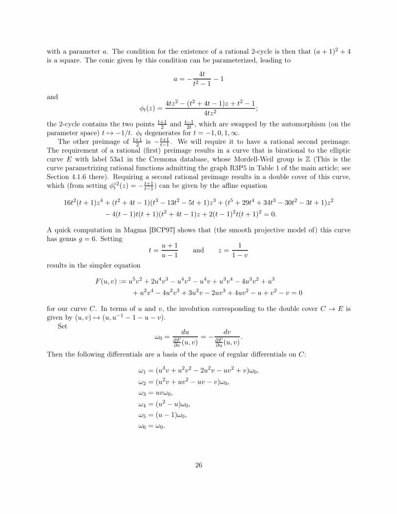
t−1 . We will require it to have a rational second preimage.The requirement of a rational (first) preimage results in a curve that is birational to the ellipticcurve E with label 53a1 in the Cremona database, whose Mordell-Weil group is Z (This is thecurve parametrizing rational functions admitting the graph R3P5 in Table 1 of the main article; seeSection 4.1.6 there). Requiring a second rational preimage results in a double cover of this curve,which (from setting φ◦2t (z) = − t+1

t−1) can be given by the affine equation

16t2(t+ 1)z4 + (t2 + 4t− 1)(t3 − 13t2 − 5t+ 1)z3 + (t5 + 29t4 + 34t3 − 30t2 − 3t+ 1)z2

− 4(t− 1)t(t+ 1)(t2 + 4t− 1)z + 2(t− 1)2t(t+ 1)2 = 0.

A quick computation in Magma [BCP97] shows that (the smooth projective model of) this curvehas genus g = 6. Setting

t =u+ 1

u− 1and z =

1

1− v

results in the simpler equation

F (u, v) := u5v2 + 2u4v3 − u4v2 − u4v + u3v4 − 4u3v2 + u3

+ u2v4 − 4u2v3 + 3u2v − 2uv3 + 4uv2 − u+ v2 − v = 0

for our curve C. In terms of u and v, the involution corresponding to the double cover C → E isgiven by (u, v) 7→ (u, u−1 − 1− u− v).

Set

ω0 =du

∂F∂v (u, v)

= −dv

∂F∂u (u, v)

.

Then the following differentials are a basis of the space of regular differentials on C:

ω1 = (u3v + u2v2 − 2u2v − uv2 + v)ω0,

ω2 = (u2v + uv2 − uv − v)ω0,

ω3 = uvω0,

ω4 = (u2 − u)ω0,

ω5 = (u− 1)ω0,

ω6 = ω0.

26

The projective closure D of the image of the corresponding canonical map C → P5 (with coordinatesw1, . . . , w6) is then defined by the following six quadratic equations:

−w2w5 + w1w6 = 0,

−w2w4 + w1w5 + w2w5 = 0,

−w25 + w4w6 − w5w6 = 0,

−w23 − w3w4 + w1w6 + w2w6 + w3w6 = 0,

w21 + 2w1w2 − w1w4 −w2w4 + w2

4 − w1w5 + w4w5 = 0,

w1w2 + 2w22 − w2w4 − w2w5 + w4w5 + w2

5 − w1w6 − w2w6 + w4w6 + w5w6 = 0.

The birational map D → C is given by

u =w4 + w5 +w6

w5 + w6, v =

w3

w5 + w6.

Using the PointSearch command of Magma, we find the following nine rational points on D:

P1 = (0 : 0 : 0 : 2 : −2 : 1),

P2 = (0 : 0 : 1 : 0 : 0 : 1),

P3 = (0 : 0 : −1 : 2 : −2 : 1),

P4 = (0 : 0 : 0 : 0 : −1 : 1),

P5 = (1 : −1 : 0 : 0 : −1 : 1),

P6 = (−2 : 1 : 0 : 0 : 0 : 0),

P7 = (0 : 0 : 0 : 0 : 0 : 1),

P8 = (0 : 0 : 1 : 0 : −1 : 1),

P9 = (1 : −1 : 1 : 0 : −1 : 1).

We suspect that these are all the rational points. The proof of this claim will take up the remainderof this note.

We note that the images of these points on C are (−1, 0), (1, 1), (−1, 1), (0, 0), (0, 1), a pointat infinity, (1, 0), and two times a point at infinity. Since u = −1, 0, 1,∞ gives a degenerate φ andv = ∞ gives z = 0, which also makes φ degenerate, this will imply that there are no non-degenerate φdefined over Q with the required properties.

C The Jacobian

Working with the equations for D ⊂ P5, we find that D has bad reduction (at most) at the primes3, 53 and 99 563. In each of these cases, the reduction is semistable, with a single componentin the special fiber that has one split node for p = 3, two non-split nodes each defined over F53

for p = 53, and one split node for p = 99563. (A node is split, if the two tangent directionsare defined over the field of definition of the node.) So D is semistable, and its Jacobian J hasconductor NJ = 3 · 532 · 99 563. Since D maps non-trivially to the elliptic curve E of conductor 53,

27

J is isogenous to a product E × A, where A is an abelian variety over Q of dimension 5 and withconductor NA = 3 · 53 · 99 563 = 15 830 517.

With a computation analogous to that leading to Lemma 4 in [Sto08], we find that the torsionsubgroup of J(Q) has exponent dividing 2 (we did not try to find the torsion subgroup exactly)and that the differences of the nine known rational points on D generate a subgroup isomorphicto Z2 of J(Q). So if we can show that J(Q) has rank 2, then we know generators of a subgroup offinite index (and the rank is strictly less than the genus), so we can apply the Chabauty-Colemanmethod.

Since there is little hope to perform a successful Selmer group computation on J , which wouldgive an upper bound for the rank, we follow the approach already used in [Sto08] and assume thatthe L-series of J has an analytic continuation to all of C, that the function

Λ(J, s) = Ns/2J (2π)−6sΓ(s)6L(J, s)

satisfies the functional equation Λ(J, 2 − s) = wJΛ(J, s) with the global root number wJ = ±1,and that the Birch and Swinnerton-Dyer conjecture holds for J . For the computations, it is betterto work with the L-series of A, since its conductor NA is smaller than NJ . According to Magma’simplementation of L-series, it requires the coefficients of L(A, s) up to n ≈ 105 000 for a precisionof 20 decimal digits. We find the coefficients of the Euler factors of the L-series of J up to therequired bound by counting the Fq-points on D for all prime powers q below the bound. This ismost efficiently done on the affine model C, by keeping track of the points at infinity modulo p and ofwhat happens at the singular points (and some care has to be taken at the bad primes). In this wayand after dividing by the Euler factors of E, we obtain within a few hours the relevant coefficientsfor the computation. We then check (using Magma’s CheckFunctionalEquation) that the data wehave computed is compatible with the expected functional equation for L(A, s) with root numberwA = −1 (but not with wA = 1). So we can safely assume that L(J, s) satisfies the functionalequation with root number wJ = wAwE = (−1)(−1) = 1. This is also in agreement with theexpectation that the global root number should be equal to the product of the local root numbers,which in the semistable case is (−1)g+s, where s is the total number of Frobenius orbits of splitnodes. Here g = 6 and s = 2, so the root number should indeed by 1. We then evaluate the derivativeof L(A, s) at s = 1 numerically and find a clearly nonzero value of ≈ 0.026803015530623712948.So according to the BSD conjecture, the rank of A(Q) should be 1 and the rank of J(Q) shouldtherefore be 2.

D Applying the Chabauty-Coleman method

By the results of the previous section (assuming BSD for J), we now know that the differencesof the known rational points provide us with generators of a finite-index subgroup of J(Q). Toapply Chabauty-Coleman, we have to fix a prime p. We choose p = 5, because 5 is a prime ofgood reduction and the set of known rational points maps bijectively to the points in D(F5) underreduction. This latter observation implies that it will be enough to show that each residue classmod 5 in D(Q5) contains at most one rational point. By the results of [Sto06], this follows whenwe can show that for each point in D(F5), there is a differential in the annihilator of J(Q) whosereduction mod 5 does not vanish there.

We first have to find a basis of this annihilator in the space of regular differentials on D over Q5.We first fix one of our known rational points P as a base-point; we have to choose it in such a

28

way that its reduction P mod 5 is non-special in the sense that the Riemann-Roch space of 6Pis one-dimensional. We check that P4 satisfies this requirement. We then use the reduction mapJ(Q) → J(F5) to find two independent points in its kernel, which we represent by divisors of theform Dj −6P4, where D1 and D2 are effective of degree 6. Since P4 is non-special, it follows that Dj

reduces mod 5 to 6P4 for j = 1, 2. We choose t = 1 + w5/w6 as a uniformizer at P4 (that reducesto a uniformizer at P4), express the differentials ω1, . . . , ω6 as power series in t times dt, integrateformally, and use the method explained in [Sto08] to compute the relevant integrals modulo 53

(modulo 52 would actually be sufficient). They are all multiples of 5, so we divide them by 5 andreduce the 2× 6-matrix obtained modulo 5. Its kernel gives the reduction of annihilator, which inour case is generated by the reductions of ω1 +ω4, ω2 −ω4, ω5 and ω6. Since the locus of vanishingof a linear combination of the ωj on D is given by the corresponding hyperplane section, all we haveto do is to check that the line defined in P5

F5by w1 + w4 = w2 − w4 = w5 = w6 = 0 does not meet

DF5, which is easily verified. This concludes the proof.

References to the Appendix

[BCP97] Wieb Bosma, John Cannon, and Catherine Playoust, The Magma algebra system. I. The user language, J.Symbolic Comput. 24 (1997), no. 3-4, 235–265. ↑26

[Sto06] Michael Stoll, Independence of rational points on twists of a given curve, Compos. Math. 142 (2006), no. 5,1201–1214, DOI 10.1112/S0010437X06002168. MR2264661 ↑28

[Sto08] , Rational 6-cycles under iteration of quadratic polynomials, LMS J. Comput. Math. 11 (2008),367–380, DOI 10.1112/S1461157000000644. MR2465796 ↑25, 28, 29

29