Introduction to QTools

QTools tutorial

Installation

1) Double click on QTools.exe2) Follow the installation

instruction3) Start QTools

Registration

1) Enter registration keyText string stored in file:CD:/Qtools/Program/TemporaryRegistration Key

3gRCb5nqV0256gVDTsqt

3gRCb5nqV0256gVDTsqt

2) Click Register Now!

Qtools Tutorial-Viscoelastic modeling-

12 Easy steps to your firstViscoelasic model of QCM-D

data

Viscoelastic model

�f=f1(n,�f,�f,�f,�f) �D=f2(n,�f,�f,�f,�f)

Crystal

Adlayer(� f, ηf, µf)

df

Fluid(� l, ηl) n=1

n=3

n=...

Voinova et al., Physica Scripta 59 (1999) 391

G = G' + jG'' = m + j2�fη

�: density, (kg/m3)

�: viscosity (G’’/�), (kg/ms)

�: elasticity (G’), (Pa)

�: thickness, (m)

Step 1

1) Click Open file

2) Choose “2stepadsorp.qsd”

3) Click open

Step 2

1) Click “OK”

3) Click “Yes”This window only appears the first time that the program is used.

4) Click “Save”This window only appears the first time that the program is used.

2) Start the modeling center, Ctrl+M

Step 3

Modeling window Data plot window

3) Layers in model

1) Viscoelastic representation2) Input data

Global parameter limits

Message box

Step 41) Click selector tool

+

2) Use selector tool to mark desired baseline row

Step 5

1) Switch to data set

2) Scroll down to marked row

3) Left click on marked row

4) Right click on marked row

5) Click Offset Columns6) Exclude time and temperature

7) Click Offset

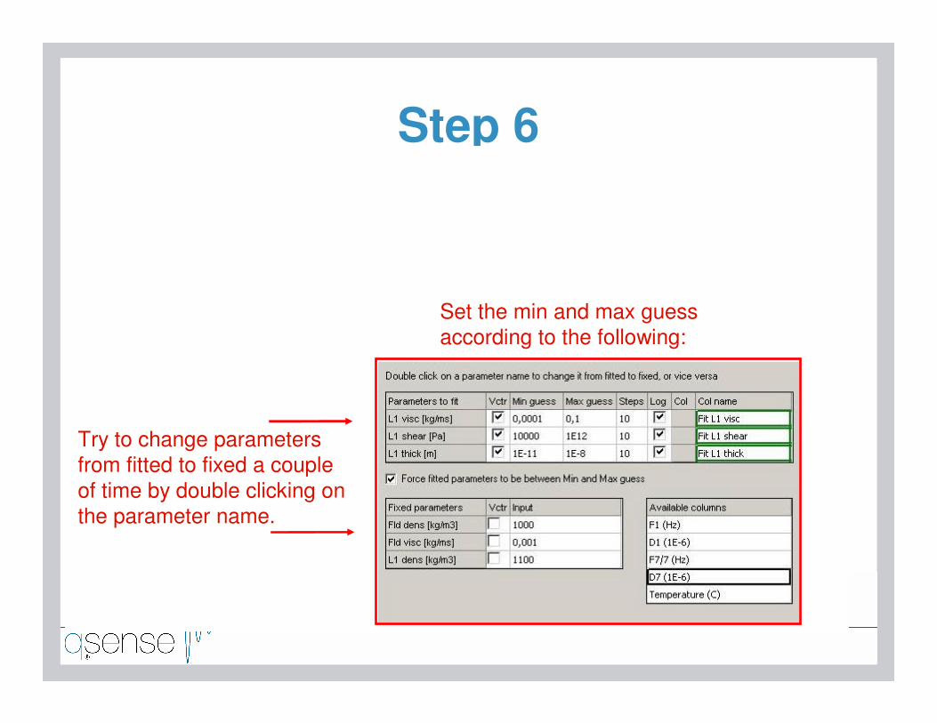
Step 6

Fitted parameters

Fixed parameters

Available columns

1) Double click on column name to change between fitted and fixed

2) Set variable form and range

Try to change parameters from fitted to fixed a couple of time by double clicking on the parameter name.

Set the min and max guess according to the following:

Step 7

Independent variable

Measured variables

Standard deviationestimate

1) Click on “Estimate all”

Step 8

Fit settings

2) Select “Limit x-values”

3) Drag selector tool to marked row

1) Select “Grid fit only first row..”

Excluded data

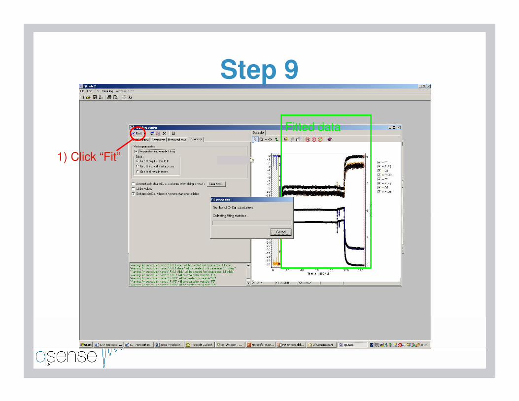
Step 9

1) Click “Fit”

Fitted data

Step 10

1) Switch to data set

2) Select Double Y plot

3) Select: X - time Y1 – Fit L1 ShearY2 – Fit L1 Visc

4) Minimize plot window

Step 11

1) Select Sauerbrey

2) Select Thickness

3) Select f data

4) Set density “1000”

5) Type new column name“Sauerbrey thickness”

6) Click “Calculate”7) Click OK

Step 12

1) Scroll to upper right corner of data set

2) Select Line plot

3) Select: X - time Y1 – Fit L1 ThickY1 – Sauerbrey Thickness

Sauerbrey thicknessViscoelastic model failure

End

---End of Viscoelastic modeling tutorial ---

---End of Viscoelastic modeling tutorial ---

Qtools Tutorial-Kinetic modeling-

• 17 Easy steps to your first kinetic model with QCM-D data

Experimental background

2:nd Q-Sense User Meeting, October 9-10 2003, Karlsruhe

Reservoir

Sensorcell

Sensor out

Inlet

Control valve

T-loop

Slow Flow – Liquid Transport

speed(ml/min) 0.03

Pump

ml

1

2

F3/3 (Hz)D3 (1E-6)

Testdata kinetic2wfit: 2003-09-30 15:33:00

Time (min)������������������������������������������������

F3/3

(H

z)

�

��

��

��

��

��

��

�

�

��

���

���

���

���

���

D3 (1E-6)

�

�

�

Tutorial

Part I

Determination of koff with QTools(Thickness, dissipation & frequency )

Part II

Determination of KA and kon

Langmuir isotherm - assumption

tofftBon RkRRCkdtdR −−= )( max

1)(,0),( max +

==∞=→∞→CK

CKRRtR

dtdR

tA

Aeq

)1()( )( tkCkeq

offoneRtR +−−=tk

eqoffeRtR −=)(

R(t) – binding at time t, Rmax the maximum binding, C concentration of B, rate of binding:

Adsorption

Desorption R(t=0)=0

Assumptions:1) Reversible adsorption2) Finite number of adsorption sites3) All sites are equal

B

BS

B+S BSkon

koff

[ ][ ][ ] off

onA k

kSB

BSK ==

Qtools kinetic tutorialPart I

Determination of koff with QTools(Thickness, dissipation & frequency )

F3/3 (Hz)D3 (1E-6)

Testdata kinetic2wfit: 2003-09-30 15:33:00

Time (min)������������������������������������������������

F3/3

(H

z)

�

��

��

��

��

��

��

�

�

��

���

���

���

���

���

D3 (1E-6)

�

�

�

tkeq

offeRtR −=)(

Desorption phase

fR

DR

R

=== δ

Adsorption phase

)1()( )( tkCkeq

offoneRtR +−−=

Part I

Step 1

1) Click Open file

2) Choose “Kinetic data.qtd”Pre edited Qtools file

3) Click open

Step 2

1) Click Open file

2) Click the drop down menu,Chose kinetic equation

Global model parameters

Functional form

0

0,2

0,4

0,6

0,8

1

1,2

1,4

0 2 4 6 8 10 12

Time

Par

amet

er A*e(-k(t-T0)))+Offsett

A+Offset

Offset

Step 3

Variable control

Fit L1 thick

1) Drag “Fit L1 Thick” to “Meas. values”Drag “Fit Kinetic thick” to “Fitted values”

Step 4

1) Double click on “A” and “k_a”.

Fitted parameters

Fixed parameters

2) Double click on Y-axis

3) Change Y-axis (left) to maximum 4

Step 5

1) Click “Limit x-values”2) Drag selector tool to start of desorption phase

3) Set variables and parameters

Functional form

0

0,2

0,4

0,6

0,8

1

1,2

1,4

0 2 4 6 8 10 12

Time

Par

amet

er A*e(-k(t-T0)))+Offsett

A+Offset

Offset

4) Click Fit All

Step 6

1) Note parameter values

Fitted data

Parameters

Step 71) Drag “D3 (1E-6)” to “Meas. values”

Drag “Fit Kinetic Dissipation” to “Fitted values”

Step 8

1) Set variables and parameters

Functional form

0

0,2

0,4

0,6

0,8

1

1,2

1,4

0 2 4 6 8 10 12

Time

Par

amet

er A*e(-k(t-T0)))+Offsett

A+Offset

Offset

2) Click Fit All

Step 9

1) Note parameter values

Fitted data

Parameters

Step 10

1) Drag “f3/3” to “Meas. values”Drag “Fit Kinetic Frequency” to “Fitted values”

2) Double click on axis

3) Change to “Automatic”

Step 11

1) Set variables and parameters

2) Click Fit All

-2,5

-2

-1,5

-1

-0,5

00 2 4 6 8 10 12

Aexp(-k_A*(t-T_0))+Offsett

Offset

A+Offset

Step 12

1) Note parameter values

Fitted data

Parameters

End of Part I

Results

Response koff

Thickness 3,75*10-4

Dissipation 3,38*10-4

Frequency 4,95*10-4

Qtools kinetic tutorialPart II

Determination of kon with Qtools(Thickness, dissipation & frequency )

F3/3 (Hz)D3 (1E-6)

Testdata kinetic2wfit: 2003-09-30 15:33:00

Time (min)������������������������������������������������

F3/3

(H

z)

�

��

��

��

��

��

��

�

�

��

���

���

���

���

���

D3 (1E-6)

�

�

�

tkeq

offeRtR −=)(

Desorption phase

fR

DR

R

=== δ

Adsorption phase

)1()( )( tkCkeq

offoneRtR +−−=

Part II

fR

DR

R

=== δ

Method

1)(,0),( max +

==∞=→∞→CK

CKRRtR

dtdR

tA

Aeq

maxmax

maxmax1

,1

1

RKm

Rk

mkxy

RKRC

RC

A

Aeq ==���

��

�

��

��

�

+=

+= C

C/Req

k

m

1) User model

2) Fit to straight line

3) Calculate kinetic coefficients

Step 13

1) Start User model

Step 14

1) Enter the following equation

Y(x)=X/P0+1/(P0*P1)

maxmax

maxmax1

,1

1

RKm

Rk

mkxy

RKRC

RC

A

Aeq ==���

��

�

��

��

�

+=

+=

Step 151) Drag “Concentration” to “Independent variable”

Drag “Concentration/Thickness” to “Measured value”Type “Fit Conc./Thick.” in fitted vaules

Step 16

1) Double click on column name to change between fitted and fixed

1) Click fit all

2) Set P0 and P1 to be fitted

Step 17

2) Repeat step 15 and 16 for D3 and F3/3

P0=RmaxP1=KAkon=KA*koff

1) Note values and calculate kon with results from Part I

End of part IIResults

Response kon koff KA

Thickness 18 3,8*10-4 4,9*104

Dissipation 19 3,4*10-4 5,8*104

Frequency 14 5,0*10-4 2,8*104

Which response (f, D or thickness) describes the amount of ”binding” best?

Frequency – Underestimates mass (thickness) in Dissipative system

Dissipation – Measure of losses, viscoelastic properties

Mass (thickness) – Most correct estimation of ”binding”