qos provisioning strategy for qos-unaware applications in...
TRANSCRIPT

IJCSNS International Journal of Computer Science and Network Security, VOL.10 No.5, May 2010
261
Manuscript received May 5, 2010 Manuscript revised May 20, 2010
QoS Provisioning Strategy for QoS-Unaware Applications in an IntServ/DiffServ Interoperating Network
Teerapat Sanguankotchakorn†, Senior Member IEEE and Ruenun Urwijitaroon† †
†School of Engineering and Technology, Asian Institute of Technology, Thailand † †Huawei Technologies (Thailand) Co., Ltd.
Summary Due to the demands for variety of services in the Internet, the quality assurance and reliability in IP network have been increasingly important. DiffServ is a scalable QoS-enabled architecture proposed to be an Internet core network. The network has to provide both new QoS-aware and legacy QoS-unaware applications with appropriate resources provisioning. Admission control is a key component to achieve this goal. However, most of the proposed admission control algorithms support only QoS-aware applications, even though most of the current Internet applications are QoS-unaware. This work proposes an admission control algorithm for providing QoS guaranteed services to QoS-aware applications and special marking to QoS-unaware applications when the network is in light-load situation. The proposed algorithm utilizes the analyzable curve-based calculation for both admission control and special marking decision. The simulation results show that the proposed algorithm can provide the deterministic QoS guarantees to QoS-aware applications as well as QoS-unaware applications without any QoS degradation. Key words: Call Admission Control, DiffServ, IntServ, QoS.
1. Introduction
1.1 Background
The current Internet architecture is best-effort service provision. However, with requirement on emerging real-time applications, such as Internet telephony and video-conferencing, the Internet QoS (Quality of Service) provisioning has become more important. To address this problem, two major mechanisms have been developed and proposed by the Internet Engineering Task Force (IETF): Integrated Services (IntServ) and Differentiated Services (DiffServ). To date, IntServ has been developed for supporting two classes of applications [1]: Real-time applications (with strict bandwidth and latency requirements) and Elastic applications (with less significance in latency requirements). IntServ model works on per-flow mechanism and it provides QoS guarantee by reserving requested resource along the
path of the flow by means of Resource ReSerVation Protocol (RSVP). While IntServ has attractions on providing deterministic end-to-end QoS guarantee, it obviously embraces two problems [2]. First, IntServ model is a connection-oriented QoS model which is not suitable for Internet short-lived flow. Moreover, end-to-end resource reservation causes the interdomain problem. Second, IntServ model has the scalability problem because all routers have to maintain the state of each flow traverses on them. An alternative concept for a scalable QoS supporting Internet is DiffServ model. The basic idea of DiffServ is to aggregate the flows into limited number of service classes depending on their service requirements by using Differentiated Service Code Point (DSCP) in the Type of Service (ToS) byte of IP headers. In order to overcome scalability problem, only boundary routers process traffic on a per-flow basis and aggregate the flows with similar QoS requirement into the same Per-Hop Behavior (PHB). Core routers only forward packets based on their PHBs. Since there is no need to maintain per-flow states in the core routers, DiffServ is more scalable than IntServ. However, DiffServ cannot provide stringent end-to-end QoS guarantees to an individual flow because of best-effort treatment within a service class [3]. In this work, we propose the scheme to provide QoS guarantee in interoperation approach of IntServ/DiffServ model for QoS-aware applications and QoS-unaware applications by special marking method. The basic idea is to use DiffServ as the core network and IntServ as the access network while admission control is implemented as border router between IntServ and DiffServ domain. The proposed algorithm utilizes the curve-based calculation for both admission control and marking decision. This paper is structured as follows: Section 2 deal with the preliminary and general concept, Section 3 explains the proposed scheme; Section 4 illustrates the simulation results while Section 5 concludes the works. All detailed proof of the formula can be found at Appendix.
IJCSNS International Journal of Computer Science and Network Security, VOL.10 No.5, May 2010
262
2. Preliminary and the Proposed General Concept
2.1 Analytical Network Model
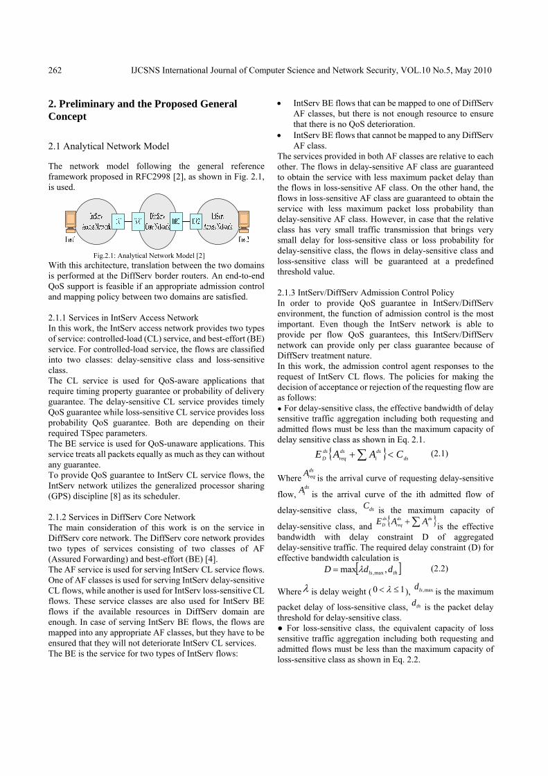
The network model following the general reference framework proposed in RFC2998 [2], as shown in Fig. 2.1, is used.
Fig.2.1: Analytical Network Model [2] With this architecture, translation between the two domains is performed at the DiffServ border routers. An end-to-end QoS support is feasible if an appropriate admission control and mapping policy between two domains are satisfied. 2.1.1 Services in IntServ Access Network In this work, the IntServ access network provides two types of service: controlled-load (CL) service, and best-effort (BE) service. For controlled-load service, the flows are classified into two classes: delay-sensitive class and loss-sensitive class. The CL service is used for QoS-aware applications that require timing property guarantee or probability of delivery guarantee. The delay-sensitive CL service provides timely QoS guarantee while loss-sensitive CL service provides loss probability QoS guarantee. Both are depending on their required TSpec parameters. The BE service is used for QoS-unaware applications. This service treats all packets equally as much as they can without any guarantee. To provide QoS guarantee to IntServ CL service flows, the IntServ network utilizes the generalized processor sharing (GPS) discipline [8] as its scheduler. 2.1.2 Services in DiffServ Core Network The main consideration of this work is on the service in DiffServ core network. The DiffServ core network provides two types of services consisting of two classes of AF (Assured Forwarding) and best-effort (BE) [4]. The AF service is used for serving IntServ CL service flows. One of AF classes is used for serving IntServ delay-sensitive CL flows, while another is used for IntServ loss-sensitive CL flows. These service classes are also used for IntServ BE flows if the available resources in DiffServ domain are enough. In case of serving IntServ BE flows, the flows are mapped into any appropriate AF classes, but they have to be ensured that they will not deteriorate IntServ CL services. The BE is the service for two types of IntServ flows:
• IntServ BE flows that can be mapped to one of DiffServ AF classes, but there is not enough resource to ensure that there is no QoS deterioration.
• IntServ BE flows that cannot be mapped to any DiffServ AF class.
The services provided in both AF classes are relative to each other. The flows in delay-sensitive AF class are guaranteed to obtain the service with less maximum packet delay than the flows in loss-sensitive AF class. On the other hand, the flows in loss-sensitive AF class are guaranteed to obtain the service with less maximum packet loss probability than delay-sensitive AF class. However, in case that the relative class has very small traffic transmission that brings very small delay for loss-sensitive class or loss probability for delay-sensitive class, the flows in delay-sensitive class and loss-sensitive class will be guaranteed at a predefined threshold value. 2.1.3 IntServ/DiffServ Admission Control Policy In order to provide QoS guarantee in IntServ/DiffServ environment, the function of admission control is the most important. Even though the IntServ network is able to provide per flow QoS guarantees, this IntServ/DiffServ network can provide only per class guarantee because of DiffServ treatment nature. In this work, the admission control agent responses to the request of IntServ CL flows. The policies for making the decision of acceptance or rejection of the requesting flow are as follows: ● For delay-sensitive class, the effective bandwidth of delay sensitive traffic aggregation including both requesting and admitted flows must be less than the maximum capacity of delay sensitive class as shown in Eq. 2.1. { } ds
dsi
dsreq
dsD CAAE <+∑ (2.1)
WheredsreqA is the arrival curve of requesting delay-sensitive
flow,dsiA is the arrival curve of the ith admitted flow of
delay-sensitive class, dsC is the maximum capacity of
delay-sensitive class, and { }∑+ dsi
dsreq
dsD AAE is the effective
bandwidth with delay constraint D of aggregated delay-sensitive traffic. The required delay constraint (D) for effective bandwidth calculation is [ ]thls ddD ,max max,λ= (2.2)
Whereλ is delay weight ( 0 1λ< ≤ ), ,maxlsd is the maximum
packet delay of loss-sensitive class, thd is the packet delay threshold for delay-sensitive class. ● For loss-sensitive class, the equivalent capacity of loss sensitive traffic aggregation including both requesting and admitted flows must be less than the maximum capacity of loss-sensitive class as shown in Eq. 2.2.

IJCSNS International Journal of Computer Science and Network Security, VOL.10 No.5, May 2010
263
{ } lslsi
lsreq
lsL CAAF <+∑ (2.3)
WherelsreqA is the arrival curve of requesting loss-sensitive
flow,lsiA is the arrival curve of the ith admitted flow of loss-
sensitive class, lsC is the maximum capacity of loss-sensitive
class, and { }∑+ lsi
lsreq
lsL AAF is the equivalent capacity with
loss constraint L of aggregated loss-sensitive traffic. The required packet loss constraint (L) for equivalent capacity calculation is [ ]thds llL ,max max,γ= (2.4)
Where γ is the loss weight ( 0 1γ< ≤ ), ,maxdslis the
maximum loss probability of delay-sensitive class, thl is the loss probability threshold for loss-sensitive class. For both classes, the constraints used in calculating effective bandwidth and equivalent capacity are depending on the amount of traffic accepted in another class. These constraints are calculated for guaranteeing less delay and loss probability of delay- and loss-sensitive classes, respectively. In case that the relative class has very small traffic admitted, the threshold value will be used as the calculation constraint. The procedure of Flow Admission Control (AC) algorithm can be illustrated as shown in Fig. 2.2.
Fig.2.2 Proposed Flow Admission Control Algorithm
2.1.4 Best-effort (BE) Traffic Promotion Policy QoS-unaware applications are normally treated as BE which will be accepted and forwarded by DiffServ network as much as possible. Normally, in traditional DiffServ network, all BE traffics will be marked as default PHB which is the lowest priority forwarding treatment. However, based on our proposed scheme, when BE traffic enters DiffServ domain, the network will perform the AC process but with different algorithm than CL flows. The AC algorithm for BE traffic is used for marking the IntServ BE traffic to appropriate DiffServ PHB rather than the default PHB. In BE marking process, Multi-Field (MF) classifier is used in this model. The MF classifier uses five parameters in packet header, namely source and destination addresses, source and destination ports, and protocol ID and the knowledge of available resources at that time to mark the packets into the
appropriate DiffServ PHB. The IntServ BE packets can be classified to AF or BE class based on the following rules: ● The BE packets will be marked into DiffServ delay-sensitive class if and only if the source and destination ports identify that the application requires timely QoS service and available resources within delay-sensitive AF PHB is enough to ensure that the delay-sensitive CL flows using that AF PHB will not be deteriorated. ● The BE packets will be marked into DiffServ loss-sensitive class if and only if the source and destination ports identify that the application requires probability of delivery QoS service and available resources within loss-sensitive AF PHB is enough to ensure that the service to loss-sensitive CL flows will not be deteriorated. ● Otherwise, the packets will be served in BE class in DiffServ domain. By these BE marking rules, the BE traffic can be promoted to higher priority DiffServ class and can receive better service when the load is light in the network. The BE promotion policy is summarized as shown in Fig. 2.3.
Fig.2.3 Proposed Best-effort (BE) Packet Marking Policy
2.2 Mathematical Analysis
2.2.1 IntServ Controlled-load (CL) As mentioned in Section 2.1.1, the IntServ network is assumed to utilize the concept of Generalized Processor Sharing (GPS) as its scheduling policy. By the concepts of GPS [7] and network calculus [5], the three fundamental bounds of particular controlled-load flow traverses the GPS which is implemented as IntServ network can be derived. a) GPS Service Analysis In order to analyze the output curve, delay, and backlog bound of IntServ flow traversing the GPS network, the service curve of GPS system has to be firstly analyzed. By work conserving concept of GPS and the service characteristic, the service curve of GPS system depends on number of flows in busy and idle period. The service-curve of GPS system can be expressed as general form of piecewise linear functions as follows: (detailed proof in Appendix A)
IJCSNS International Journal of Computer Science and Network Security, VOL.10 No.5, May 2010
264
( ) .,...,2,1,;
)()()(
1
1
01
11
Nkttttssts
tSttstS
kk
k
jjjjk
kukku
=∀≤<−−=
+−=
−
−
=+
−−
∑
(2.5)
where ( )uS t is the universal service curve which is identical
in all flows, ( ) ( ) kiiu titStS ,∀= φ is the time such that the thk flow ends its busy period, ks is the universal slope of ( )uS t in the region of 0, 01 =≤<− tttt kk and 0 0s = .
b) IntServ Controlled-load (CL) Analysis In this work, the IntServ/DiffServ AC agent uses the output curve of the IntServ flow as the arrival curve to calculate the resource requirement. Combining the GPS universal service curve equation and network calculus basic, the output curve, delay, and backlog bound can be derived. The output curve of IntServ flows can be classified into three different cases: (1) The slope of the service case is always greater than traffic token rate (2) The slope of the service case is greater or equal to traffic token rate (3) The traffic token rate is always greater than the slope of service case (detailed proof in Appendix B). Regarding delay and backlog bound calculation; delay bound can be expressed as the maximum horizontal distance between arrival and output curve, while backlog bound can be expressed as the maximum vertical deviation between arrival and output curve. 2.2.2 Admission Control Resource Calculation The traffic arrival to DiffServ network, both delay- and loss-sensitive classes, can be constrained by the aggregation of output curve of IntServ controlled-load flows. As mentioned in Section 2.2.1, the IntServ’s output flows can be classified into three different cases. However, the output curves of IntServ flow are piecewise linear functions in all cases. Hence, the output curve of IntServ flow being considered as per-flow arrival curve of DiffServ network can be rewritten as
*0
* * *1 0 1
* * * * * *2 1 1 1 2*
* * * * * *1 1 1
* * * * *1
0 ........
( ) ( ) ....( )
( ) ( ) ........( ) ( )
ii
N N i N N N
N N i N N
ta t t
a t A tA t
a t A t
a t A t
τ
τ ττ τ τ τ
τ τ τ τ
τ τ τ− − −
+
⎧ ≤⎪
< ≤⎪⎪ − + < ≤⎪= ⎨⎪⎪ − + < ≤⎪⎪ − + >⎩
M M
(2.10)
where * * * *1 2 1, , , ,N Na a a a +K are slope of output-curves of
IntServ flows, and* * * *0 1 2, , , , Nτ τ τ τK are the time such that the
slope of IntServ output curve changes. The DiffServ arrival
curve of aggregate IntServ flows ( DSA ) which is the summation of all per-flow arrival curve can be expressed as
0
1 0 1
2 1 1 1 2
1 1 1
1
0 ........
( ) ( ) ....( )
( ) ( ) ....( ) ( ) ....
DSDS
K K DS K K K
K K DS K K
ta t t
a t A tA t
a t A ta t A t
ττ τ
τ τ τ τ
τ τ τ ττ τ τ− − −
+
≤⎧⎪ < ≤⎪⎪ − + < ≤⎪= ⎨⎪⎪ − + < ≤⎪
− + >⎪⎩
M M
(2.11)
where 1 2 1, , , ,K Ka a a a +K are slope of aggregate arrival
curve of DiffServ network, and 0 1 2, , , , Kτ τ τ τK are the time such that the slope of arrival curve changes. Resource Required for Delay-sensitive Class For delay-sensitive AF class, the required resource to guarantee the maximum packet delay D is characterized by aggregate effective bandwidth (detailed proof in Appendix C):
⎭⎬⎫
⎩⎨⎧
∈∀+
= + KiD
VaE dsi
dsids
KdsD ,...,2,1,max 1 τ
(2.12)
wheredsDE is the effective bandwidth of delay-sensitive
class, 1dsKa + is the long term slope of arrival curve which equals
the summation of token bucket rate of all delay-sensitive
flows, and ds
iV is the amount of bits arrival at critical
timedsiτ .
a) Resource Required for Loss-sensitive Class For loss-sensitive AF class, the required resource to guarantee the maximum packet loss probability L is characterized by aggregate equivalent capacity (detailed proof in Appendix C):
⎭⎬⎫
⎩⎨⎧
∈∀−−
= + KiQVLaF lsi
lsls
ilsK
lsL ,...,2,1)1(,max 1 τ
(2.13)
wherels
LF is the equivalent capacity of loss-sensitive class, 1
lsKa + is the long term slope of arrival curve which is equal to
the summation of token bucket rate of all loss-sensitive flows,
lsiV is the amount of bit arrival at critical time
lsiτ ,and lsQ is
the maximum buffer size of loss-sensitive class. 2.2.3 Available Resource for Best-effort Promotion In order to promote BE packet into appropriate higher priority class without QoS deterioration, the available

IJCSNS International Journal of Computer Science and Network Security, VOL.10 No.5, May 2010
265
resource of higher priority class guaranteeing the required QoS service has to be calculated. The high priority available resource that can be used for serving BE traffic is again calculated based on the concept of effective bandwidth and equivalent capacity. Regarding the BE traffic that can be promoted to delay-sensitive AF class, the available resource for promotion is calculated using effective bandwidth and can be expressed as (detailed proof in Appendix D):
1( )min , 1, 2, ,
ds dsbe ds i ds iD ds K ds
i
D C VR C a i Kττ+
⎧ ⎫+ −= − ∀ ∈⎨ ⎬
⎩ ⎭K
(2.14)
where beDR is the available bandwidth of delay-sensitive class
that can serve the promoted BE packets and dsC is the maximum capacity of the delay-sensitive class. Regarding the BE traffic that can be promoted to loss-sensitive AF class, the available resource for promotion is calculated using equivalent capacity which can be expressed as (detailed proof in Appendix D):
(1 )min 1, 2, ,(1 )
ls lsbe ls i ls iL ds
i
C Q L VR i KL
ττ
⎧ ⎫+ − −= ∀ ∈⎨ ⎬−⎩ ⎭
K
(2.15)
wherebeLR is the available bandwidth of loss-sensitive class
that can serve the promoted BE packets and lsC is the maximum capacity of the loss-sensitive class. The available bandwidth for promotion is used as the maximum rate that the BE packets can be marked as AF service. Even though, the limit of maximum BE promotion rate can guarantee the non-degradation of the actual AF traffic’s QoS, however, there is no prediction of the forthcoming AF arrivals. If the new AF flows simultaneously request for their services, the QoS may be deteriorated. In order to avoid this situation, three additional conditions are also used as BE promotion policy: (1) The BE traffic cannot be marked as AF class if the effective bandwidth or equivalent capacity of traditional AF traffic is more than the half of maximum capacity. (2) The BE traffic cannot be marked as AF class if the queue length of AF class is more than the half of maximum buffer size. (3) The BE traffic cannot be marked as AF class if the cumulative average queue rate of AF class reaches the reserved effective bandwidth or equivalent capacity.
3. Proposed Scheme Simulation Model
3.1 Proposed Scheme Simulation
For validity verification, Network Simulator (NS-2) [10] is used as a tool to simulate the proposed algorithm. 3.1.1 Simulation Network Model and Parameters The network model used in simulation follows the analytical network model as illustrated in Fig. 2.1. Since this work focuses only on the AC at DiffServ border routers, the network model can be actually simplified to the one shown in Fig. 3.1.
Fig.3.1 Simplified Network Model
In simulation model, the IntServ networks are assumed to be merged in the source and destination hosts. The source hosts will generate three types of traffic: delay-sensitive CL service, loss-sensitive CL service, and BE (QoS-unaware). For all traffic types, MPEG-4 and VBR source are used as traffic generator. In DiffServ domain, only one DiffServ core node is used for representing DiffServ cloud. The AC process is enabled at DiffServ edge node for both acceptance on QoS-aware traffic and marking on QoS-unaware traffic. Within DiffServ domain, three classes of DiffServ PHBs are used: two classes of AF, and one class of BE. 3.1.2 Performance Evaluation Criteria The performance evaluation criteria are defined as follows: ● Acceptance Probability of controlled-load ● Average Throughput (Per-class network utilization) ● Average Packet Queuing Delay ● Packet Loss Probability The comparison is done between this proposed scheme and typical IntServ/DiffServ model without admission control algorithm. 3.1.3 Network Simulator Modifications To simulate the proposed network model, four parts of NS-2 are modified or developed: DiffServ module, IntServ agent, VBR traffic source, and performance tracing tool. a) DiffServ Module The original built-in DiffServ module in NS-2 has no function of admission control. Therefore, DiffServ module is modified in two parts: Admission Control Agent (for CL requesting), and BE Marker (for BE promotion algorithm),
IJCSNS International Journal of Computer Science and Network Security, VOL.10 No.5, May 2010
266
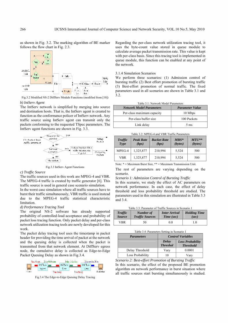
as shown in Fig. 3.2. The marking algorithm of BE marker follows the flow chart in Fig. 2.3.
Fig.3.2 Modified NS-2 DiffServ Module Functions (modified from [10])
b) IntServ Agent The IntServ network is simplified by merging into source and destination hosts. That is, the IntServ agent is created to function as the conformance policer of IntServ network. Any traffic source using IntServ agent can transmit only the packets conforming to the requested TSpec parameters. The IntServ agent functions are shown in Fig. 3.3.
Fig.3.3 IntServ Agent Functions
c) Traffic Source The traffic sources used in this work are MPEG-4 and VBR. The MPEG-4 traffic is created by traffic generator [6]. This traffic source is used in general case scenario simulation. In the worst case simulation where all traffic sources have to burst their traffic simultaneously, VBR traffic is used instead due to the MPEG-4 traffic statistical characteristic limitation. d) Performance Tracing Tool The original NS-2 software has already supported probability of controlled-load acceptance and probability of packet loss tracing function. Only packet delay and per-class network utilization tracing tools are newly developed for this work. The packet delay tracing tool uses the timestamp in packet header for providing the time arrival of packet at the network and the queuing delay is collected when the packet is transmitted from that network element. At DiffServ egress node, the cumulative delay is collected as Edge-to-Edge Packet Queuing Delay as shown in Fig.3.4.
Fig.3.4 The Edge-to-Edge Queuing Delay Tracing
Regarding the per-class network utilization tracing tool, it uses the byte-count value stored in queue module to calculate average packet transmission rate. This value is kept with per-class basis. Since this tracing tool is implemented in queue module, this function can be enabled at any point of the network. 3.1.4 Simulation Scenarios We perform three scenarios: (1) Admission control of bursting traffic (2) Best effort promotion of bursting traffic (3) Best-effort promotion of normal traffic. The fixed parameters used in all scenarios are shown in Table 3.1 and 3.2.
Table 3.1: Network Model Parameters Network Model Parameters Parameter Value Per-class maximum capacity 10 Mbps
Per-class buffer size 100 Packets
Link delay 5 ms
Table 3.2: MPEG-4 and VBR Traffic Parameters
Traffic Type
Peak Rate (bps)
Bucket Rate (bps)
MBS* (bytes)
MTU** (bytes)
MPEG-4 1,325,877 210,994 5,524 500
VBR 1,325,877 210,994 5,524 500
Note: * = Maximum Burst Size, ** = Maximum Transmission Unit.
The rest of parameters are varying depending on the scenario. Scenario 1: Admission Control of Bursting Traffic In this scenario, we study the effect of AC parameters on network performance. In each case, the effect of delay threshold and loss probability threshold are studied. The parameters used in this simulation are illustrated in Table 3.3 and 3.4.
Table 3.3: Parameter of Traffic Sources in Scenario 1 Traffic Source
Number of Traffic Sources
Inter Arrival Time (sec)
Holding Time (sec)
VBR 50 0.0 1.0
Table 3.4: Parameters Setting in Scenario 1
Parameters Control Variables
Delay Threshol
Loss Probability Threshold
Delay Threshold Vary 0.0001 Loss Probability 10 Vary
Scenario 2: Best-effort Promotion of Bursting Traffic In this scenario, the effect of the proposed BE promotion algorithm on network performance in burst situation where all traffic sources start bursting simultaneously is studied.

IJCSNS International Journal of Computer Science and Network Security, VOL.10 No.5, May 2010
267
We consider the effect of amount of CL traffic in the network instead of AC parameters as in previous scenario. The parameters used in this scenario are illustrated in Table 3.5.
Table 3.5: Parameters of Traffic Sources in Scenario 2
Traffic Number of Traffic Sources
Inter Arrival Time (sec)
Holding Time (sec)
VBR 200 0.0 1.0
For all cases, the AC parameters: delay threshold and loss probability threshold are set to 5 ms and 0.001, respectively. Scenario 3: Best-effort Promotion of Normal Traffic In this scenario, the effect of proposed BE promotion scheme in normal traffic situation is studied. The AC parameters are the same as in scenario 2. The traffic parameters are shown in Table 3.6.
Table 3.6: Parameters of Traffic Sources in Scenario 3 [6]
Traffic Number of Traffic Sources
Inter Arrival Time (sec)
Holding Time (sec)
MPEG-4 200 0.05 2.0
4. Simulation Results and Discussions
4.1 Scenario 1: Admission Control of Bursting Traffic
4.1.1 Effect of Delay Threshold on Network Performance
(a) (b)
(c) (d)
Fig.4.1 Effect of Delay Threshold on (a) Acceptance Probability (b) Average Throughput (c) Average Delay (d) Packet Loss Probability
a) Discussion of Simulation Results Fig. 4.1 (a) and (b) illustrate the same trend of results. This is because when delay threshold is very small, many effective bandwidths are required to accept one more flow. When delay threshold is large, the network cannot accommodate any more traffic. In Fig.4.1 (c), in case of Delay-sensitive class, the packet delay proportional to the number of accepted flows while in case of Loss-sensitive class, the increment of delay threshold affects packet delay. This is because of round robin scheduling manner. When delay threshold is small, a small number of Delay-sensitive packets are transmitted in the network. Therefore, the capacity in the network will be available to serve Loss-sensitive packets which results in less delay service. In Fig. 4.1 (d), the results show that if delay threshold is less than the maximum queuing delay, the network will always be able to serve all packets, then causing no queuing loss. However, if delay threshold is more than the maximum queuing delay, the Delay-sensitive traffic will be over-admitted which leads to increment of packet loss of both traffics. 4.1.2 Effect of Loss Probability Threshold on Network Performance
(a) (b)
(c) (d)
Fig.4.2 Effect of Loss Probability Threshold on (a) Acceptance Probability (b) Average Throughput (c) Average Packet Delay (d) Packet loss
Probability
a) Discussion of Simulation Results The effect of loss probability threshold on Acceptance Probability, Average throughput and Average delay (Fig. 4.2 (a)-(d)) is not so much perceptible as the effect of delay threshold. Since the requirement of loss probability
0
0.002
0.004
0.006
0.008
0.01
0.012
0.014
0.016
0.005 0.02 0.035 0.05 0.065 0.08 0.095
Ave
rage
Pac
ket
Del
ay (
seco
nd)
Packet Loss Probability Threshold
Delay Sensitive Loss Sensitive
00.0050.01
0.0150.02
0.0250.03
0.0350.04
0.045
0.005 0.02 0.035 0.05 0.065 0.08 0.095
Pac
ket
Loss
Pro
babi
lity
Packet Loss Probability Threshold
Delay Sensitive Loss Sensitive
0
1
2
3
4
5
6
7
8
0.005 0.015 0.025 0.035 0.045 0.055 0.065 0.075 0.085 0.095
Avera
ge T
raff
ic R
ate
(M
bp
s)
Delay Threshold (second)
Delay Sensitive Loss Sensitive
00.10.20.30.40.50.60.70.80.9
1
0.005 0.015 0.025 0.035 0.045 0.055 0.065 0.075 0.085 0.095
Pro
babi
lity
of A
ccep
tanc
e
Delay Threshold (second)
Delay Sensitive Loss Sensitive
00.0020.0040.0060.0080.01
0.0120.0140.0160.018
0.005 0.02 0.035 0.05 0.065 0.08 0.095
Aver
age
Pack
et D
elay
(sec
ond)
Delay Threshold (second)
Delay Sensitive Loss Sensitive
0
0.05
0.1
0.15
0.2
0.25
0.005 0.02 0.035 0.05 0.065 0.08 0.095
Pac
ket
Loss
Pro
babi
lity
Delay Threshold (second)
Delay Sensitive Loss Sensitive
00.10.20.30.40.50.60.70.80.9
1
0.005 0.015 0.025 0.035 0.045 0.055 0.065 0.075 0.085 0.095
Pro
babi
lity
of A
ccep
tanc
e
Packet Loss Probability Threshold
Delay Sensitive Loss Sensitive
0
1
2
3
4
5
6
0.005 0.015 0.025 0.035 0.045 0.055 0.065 0.075 0.085 0.095
Ave
rage
Tra
ffic
Rat
e (M
bps)
Packet Loss Probability Threshold
Delay Sensitive Loss Sensitive
IJCSNS International Journal of Computer Science and Network Security, VOL.10 No.5, May 2010
268
threshold of 10-6 or 10-5 does not much influence admission control result. However, as illustrated in Fig. 4.2 (d), only the packet loss probability of Loss-sensitive class is affected by loss probability threshold.
4.2 Scenario 2: BE Promotion of Bursting Traffic
4.1.1 Effect of BE promotion of Bursting Traffic on Network performance
(a) (b)
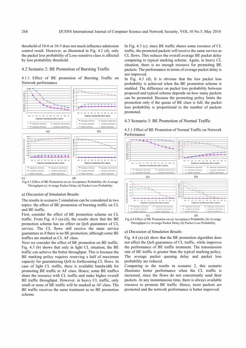
(c) (d) Fig.4.3 Effect of BE Promotion on (a) Acceptance Probability (b) Average
Throughput (c) Average Packet Delay (d) Packet Loss Probability
a) Discussion of Simulation Results The results in scenario 2 simulation can be considered in two topics: the effect of BE promotion of bursting traffic on CL and BE traffic. First, consider the effect of BE promotion scheme on CL traffic. From Fig. 4.3 (a)-(d), the results show that the BE promotion scheme has no effect on QoS guarantees of CL service. The CL flows still receive the same service guarantees as if there is no BE promotion; although some BE traffics are marked as CL AF class. Next we consider the effect of BE promotion on BE traffic. Fig. 4.3 (b) shows that only in light CL situation, the BE traffic can achieve the better throughput. This is because the BE marking policy requires reserving a half of maximum capacity for guaranteeing QoS to forthcoming CL flows. In case of light CL traffic, there is available bandwidth for promoting BE traffic to AF class. Hence, some BE traffics share the resource with CL traffic and make higher overall BE traffic throughput. However, in heavy CL traffic, only small or none of BE traffic will be marked as AF class. The BE traffic receives the same treatment as no BE promotion scheme.
In Fig. 4.3 (c), since BE traffic shares some resource of CL traffic, the promoted packets will receive the same service as CL flows. This reduces the overall average BE packet delay comparing to typical marking scheme. Again, in heavy CL situation, there is no enough resource for promoting BE packets. The performance in terms of average packet delay is not improved. In Fig. 4.3 (d), It is obvious that the less packet loss probability is achieved when the BE promotion scheme is enabled. The difference on packet loss probability between proposed and typical scheme depends on how many packets can be promoted. Because the promoting policy limits the promotion only if the queue of BE class is full, the packet loss probability is proportional to the number of packets promoted.
4.3 Scenario 3: BE Promotion of Normal Traffic
4.3.1 Effect of BE Promotion of Normal Traffic on Network Performance
(a) (b)
(c) (d) Fig.4.4 Effect of BE Promotion on (a) Acceptance Probability (b) Average
Throughput (c) Average Packet Delay (d) Packet Loss Probability
a) Discussion of Simulation Results Fig. 4.4 (a)-(d) show that the BE promotion algorithm does not affect the QoS guarantees of CL traffic, while improves the performance of BE traffic treatment. The transmission rate of BE traffic is greater than the typical marking policy. The average packet queuing delay and packet loss probability are reduced. Comparing to the results in scenario 2, this scenario illustrates better performance when the CL traffic is increased, since the flows do not concurrently send their packets. At any instantaneous time, there is always available resource to promote BE traffic. Hence, more packets are promoted and the network performance is better improved.
0
0.02
0.04
0.06
0.08
0.1
0.12
0.05 0.1 0.15 0.2 0.25 0.3 0.35 0.4 0.45 0.5 0.55 0.6
Av
era
ge
Pa
ck
et
De
lay
(se
co
nd
)
Proportion of controlled-load traffic in network
Delay Sensitive - with Promotion Delay Sensitive - without Promotion
Loss Sensitive - with Promotion Loss Sensitive - without Promotion
Best Effort - with Promotion Best Effort - without Promotion
00.05
0.10.15
0.20.25
0.30.35
0.40.45
0.05 0.1 0.15 0.2 0.25 0.3 0.35 0.4 0.45 0.5 0.55 0.6
Pa
ck
et L
os
s P
rob
ab
ility
Proportion of controlled-load traffic in network
Delay Sensitive - with Promotion Delay Sensitive - without Promotion
Loss Sensitive - with Promotion Loss Sensitive - without Promotion
Best Effort - with Promotion Best Effort - without Promotion
00.0050.01
0.0150.02
0.0250.03
0.0350.04
0.045
0.05 0.1 0.15 0.2 0.25 0.3 0.35 0.4 0.45 0.5 0.55 0.6
Av
era
ge
Pa
ck
et
De
lay (
se
co
nd
)
Proportion of controlled-load traffic in network
Delay Sensitive - with Promotion Delay Sensitive - without Promotion
Loss Sensitive - with Promotion Loss Sensitive - without Promotion
Best Effort - with Promotion Best Effort - without Promotion
0
0.1
0.2
0.3
0.4
0.5
0.6
0.7
0.05 0.1 0.15 0.2 0.25 0.3 0.35 0.4 0.45 0.5 0.55 0.6
Pa
ck
et L
os
s P
ro
ba
bilit
y
Proportion of controlled-load traffic in network
Delay Sensitive - with Promotion Delay Sensitive - without Promotion
Loss Sensitive - with Promotion Loss Sensitive - without Promotion
Best Effort - with Promotion Best Effort - without Promotion
00.10.20.30.40.50.60.70.80.9
1
0.05 0.1 0.15 0.2 0.25 0.3 0.35 0.4 0.45 0.5 0.55 0.6
Pro
ba
bilit
y o
f A
cc
ep
tan
ce
Proportion of controlled-load traffic in network
Delay Sensitive - with Promotion Delay Sensitive - without Promotion
Loss Sensitive - with Promotion Loss Sensitive - without Promotion
0
2
4
6
8
10
12
0.05 0.1 0.15 0.2 0.25 0.3 0.35 0.4 0.45 0.5 0.55 0.6
Av
era
ge
Tra
ffic
Ra
te (
Mb
ps
)
Proportion of controlled-load traffic in network
Delay Sensitive - with Promotion Delay Sensitive - without Promotion
Loss Sensitive - with Promotion Loss Sensitive - without Promotion
Best Effort - with Promotion Best Effort - without Promotion
00.10.20.30.40.50.60.70.80.9
1
0.05 0.1 0.15 0.2 0.25 0.3 0.35 0.4 0.45 0.5 0.55 0.6
Pro
ba
bili
ty o
f A
cc
ep
tan
ce
Proportion of controlled-load traffic in network
Delay Sensitive - with Promotion Delay Sensitive - without Promotion
Loss Sensitive - with Promotion Loss Sensitive - without Promotion
00.5
11.5
22.5
33.5
44.5
5
0.05 0.1 0.15 0.2 0.25 0.3 0.35 0.4 0.45 0.5 0.55 0.6
Av
era
ge
Tra
ffic
Ra
te (
Mb
ps
)
Proportion of controlled-load traffic in network
Delay Sensitive - with Promotion Delay Sensitive - without Promotion
Loss Sensitive - with Promotion Loss Sensitive - without Promotion
Best Effort - with Promotion Best Effort - without Promotion

IJCSNS International Journal of Computer Science and Network Security, VOL.10 No.5, May 2010
269
5. Conclusions
Admission control agent is the most important network element in QoS provisioning in IntServ/DiffServ interoperating network to provide QoS guarantee. In this research, the QoS provisioning algorithms used in IntServ/DiffServ environment are studied and analyzed. The class-relative QoS guarantee policy is proposed. This policy provides QoS guarantee using class service status as QoS parameter. The Delay-sensitive applications will receive less-delay service guarantee, while Loss-sensitive applications will receive less-loss service guarantee. The curve-based admission control policy used to provide these QoS guarantee is proposed and analyzed. This admission control policy utilizes the concept of effective bandwidth and equivalent capacity in resource calculation. However, with curve-based admission control, the low network utilization cannot be avoided. In this work, special marking policy for BE packets is proposed to improve the network utilization as well as the service to QoS-unaware applications. This marking policy will mark the BE packets as appropriate AF traffic if there is enough available resource on AF class to guarantee no QoS degradation. To verify the proposed schemes: class-relative admission control and BE promotion algorithm, three simulation scenarios are established. Two types of traffic source are used: MPEG-4 and VBR traffic. From simulation results, it can be concluded that the proposed admission control algorithm can provide class-relative QoS guarantees in both worst-case and normal-case situations. Regarding the BE promotion algorithm, the simulation results show that there is no effect on the service of CL traffic in both burst and normal situations. The QoS provided to Delay-sensitive and Loss-sensitive applications is not deteriorated. In light CL situation, the service provided to BE traffic is improved in terms of average packet delay and packet loss probability as well as the network utilization.
Appendix
A. Derivation of GPS Service Curve To analyze the service curve of GPS offered to IntServ CL flows. The worst case situation called “all-greedy regime” [7] is considered.
Let 1,2,...,i N= be the thi CL admitted flow. Each flow must
conform to the token bucket parameter ( , )i ib r as defined in
RFC2212 [8], where ib and ir are the bucket size and bucket
rate of thethi CL admitted flow, respectively. Hence, the
thi flow traffic transmitted to the network is
( ) min[ , ]i i i i iA t M p t b rt≤ + + for 0t ≥ (A.1)
where iM and ip are the maximum datagram size and peak rate of the
thi CL admitted flow. By the definition of CL
service, the peak rate ( )ip is not defined and it can be assumed to be the line rate of incoming interface [12]. For simplification, without loss of generality, we assume that the peak rate of flow is infinite. Hence,
( )i i iA t b rt≤ + for 0t ≥ (A.2)
Let ( )iS t denotes the service curve of thethi flow, iφ denotes
the GPS assignment (weight) of thi flow and C denotes the
GPS service capacity. The worst case scenario occurs when all sources start sending packets at their maximum rate at the
same time 0t = [7]. In this case, the arrival curve of thi
flow is
( )i i iA t b rt= + . (A. 3)
Let ( )uS t denotes the universal service curve which is
identical for all flows,itStS
i
iu ∀=
φ)()(
, kt denotes the time
such that the thk flow ends its busy period
( Nttt ≤≤≤< K210 ), ks denotes the universal slope
which is the slope of ( )uS t in the region of kk ttt ≤<−1 , kB denotes the set of flows which are still in
busy period when 1−> ktt .
Consider the time 10 tt ≤< ; all flows are in busy period. So, the service curve of each flow is
11
0;)( ttCttSN
jjii ≤<⎟⎠⎞
⎜⎝⎛= ∑
=
φφ
(A.4)
11
0;)( ttCttSN
jju ≤<⎟⎠⎞
⎜⎝⎛= ∑
=
φ
(A.5) and
⎪⎭
⎪⎬
⎫
⎪⎩
⎪⎨
⎧
=+
>=
⎭⎬⎫
⎩⎨⎧
=>=
∑=
∈
∈
N
jj
i
ii
Bi
ui
i
Bi
Cttrbt
tStAtt
1
1
:0inf
)()(:0inf
1
1
φφ
φ (A.6)
∑=
=N
jjCs
11 φ (A.7)

IJCSNS International Journal of Computer Science and Network Security, VOL.10 No.5, May 2010
270
Next, consider the time 21 ttt ≤< , the 1sti = flow already ends its busy period but still transmits packets at its token
bucket rate 1r . ( ) ( ) 2111
1 ;)()(
2
ttttSttrCtS i
Bjj
ii ≤<+−
−=
∑∈
φφ
(A.8) ( )( ) 2111
1 ;)()(
2
ttttSttrCtS u
Bjj
u ≤<+−−
=∑∈
φ (A.9)
and
⎪⎭
⎪⎬⎫
⎪⎩
⎪⎨⎧
+−−
=+
>=
⎭⎬⎫
⎩⎨⎧
=>=
∑∈
∈
∈
)()()(:0inf
)()(:0inf
111
2
2
2
2
tSttrCtrbt
tStAtt
u
Bjji
ii
Bi
ui
i
Bi
φφ
φ (A.10)
( ) ∑∈
−=2
12Bj
jrCs φ (A.11)
Then, consider the time kk ttt ≤<−1 , the thi k< flows
already end their busy period, but still transmit packet at
rate ir .
( ) kkkik
Bjj
iBj
j
i ttttSttrC
tS
k
k ≤<+−⎟⎠⎞
⎜⎝⎛ −
= −−−
∈
∉
∑
∑111 ;)()(
φ
φ
(A.12)
( ) kkkuk
Bjj
Bjj
u ttttSttrC
tS
k
k ≤<+−⎟⎠⎞
⎜⎝⎛ −
= −−−
∈
∉
∑
∑111 ;)()(
φ
(A.13) and
⎪⎪⎭
⎪⎪⎬
⎫
⎪⎪⎩
⎪⎪⎨
⎧
+−⎟⎠⎞
⎜⎝⎛ −
=+
>=
⎭⎬⎫
⎩⎨⎧
=>=
−−
∈
∉
∈
∈
∑
∑)()(:0inf
)()(:0inf
11 kuk
Bjj
Bjj
i
ii
Bi
ui
i
Bik
tSttrC
trbt
tStAtt
k
k
k
k
φφ
φ(A.14)
∑∑∈∉
⎟⎠⎞
⎜⎝⎛ −=
kk Bjj
Bjjk rCs φ (A.15)
Hence, the service curve of GPS server is
⎪⎪⎪
⎩
⎪⎪⎪
⎨
⎧
≤<+−
≤<+−
≤<+−≤<
=
−−−
−−−
NNNuNN
kkkukk
u
u
ttttStts
ttttStts
ttttSttsttts
tS
111
111
21112
11
);()(
);()(
);()(0;
)(
M
M
(A.16) And let 00 =t and 0 0s = , then (A.16) can be rewritten in simpler form as
( )∑−
=−+
−−
=∀≤<−−=
+−=1
011
11
,...,2,1,;
)()()(k
jkkjjjk
kukku
Nkttttssts
tSttstS(A.
17) B. Derivation of IntServ Controlled-Load Output Flows To analyze the output curve of IntServ flows, the definition of arrival curve, service curve, and network calculus [5] are used. The arrival curve of IntServ controlled-load flow is
( )i i iA t b rt= + and the service curve of GPS server is in (A.17). The output curve is the min-plus deconvolution between arrival and service curve:
*
0( ) ( )( ) sup{ ( ) ( )}i i i i i
uA t A S t A t u S u
≥= ∅ = + − (B.1)
Let 'k i ks sφ= be the kth slope of ith flow. Then,
( )
( )∑
∑−
=−+
−
=+
=≤<′−′−′=
−−==
1
011
1
01
,,3,2,1,;
)()(
k
jkkjjjk
k
jjjjikiuii
ikttttssts
tsststStS
K
φφφ(B.2)
( )
( )⎭⎬⎫
⎩⎨⎧ ≤<′−′+′−+=
⎭⎬⎫
⎩⎨⎧ ≤<′−′+′−++=
∑
∑−
=−+
≤≤≥
−
=−+
≤≤≥
∗
1
011
1,0
1
011
1,0
|)(sup
|)(sup)(
k
jkkjjjkii
iku
k
jkkjjjkii
ikui
tuttssusrb
tuttssusutrbtA
(B.3)
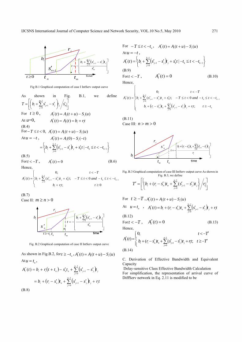
Define mt be the time such that )()( 1 miimi tSbtS <≤− , nt be
the time such that in rs >′ and let 00 =t and 00 =′s .There are three different cases of controlled-load
output curve.
Case I: ( 0)m n> = In this case, the slope of service curve is always greater than traffic token rate.
IJCSNS International Journal of Computer Science and Network Security, VOL.10 No.5, May 2010
271
nt mt
ib
ir
1+′ns( )
⎥⎥⎥
⎦
⎤
⎢⎢⎢
⎣
⎡
′
′−′+−=
∑−
=+
m
m
jjjji
s
tssbt
1
01
0≥t Fig B.1 Graphical computation of case I IntServ output curve
As shown in Fig. B.1, we define
⎥⎦
⎤⎢⎣
⎡ ′⎟⎠⎞
⎜⎝⎛ ′−′+= ∑
−
=+ mj
m
jjji stssbT
1
01
For 0t ≥ , )()()(* uSutAtA iii −+= At u=0, trbtAtA iiii +== )()(* (B.4) For ,0<≤− tT )()()(* uSutAtA iii −+= At tu −= , )()0()(* tSAtA iii −−=
( )⎭⎬⎫
⎩⎨⎧ −<≤−′+′−′+= ∑
−
=−+
1
011 |
k
jkkkjjji ttttstssb
(B.5) For Tt −< ,
*( ) 0iA t = (B.6) Hence,
⎪⎩
⎪⎨
⎧
≥+
−<≤−<≤−′+′−′+
−<
= −
−
=+∑
0;
0;)(
;0
)( 1
1
01
*
ttrb
tttandtTtstssb
Tt
tA
ii
kk
k
jkjjjii
(B.7) Case II: 0m n≥ >
ib
ir
ns ′
ntt −≥nt mt
( )
⎥⎥⎥
⎦
⎤
⎢⎢⎢
⎣
⎡
′
′−′+−=
∑−
=+
m
m
jjjji
s
tssbt
1
01
Fig. B.2 Graphical computation of case II IntServ output curve
As shown in Fig.B.2, forntt −≥ , )()()(* uSutAtA iii −+=
At ntu = ,
( ) ( )
( ) ( ) trtsstsrb
tsststtrbtA
i
n
jjjjnnii
n
jjjjnnniii
+′−′+′−+=
′−′+′−++=
∑
∑−
=+
−
=+
1
01
1
01
* )(
(B.8)
For nttT −<≤− , )()()(* uSutAtA iii −+=
At tu −= ,
( )⎭⎬⎫
⎩⎨⎧ −<≤−′+′−′+= ∑
−
=−+
1
011
* |)(k
jkkkjjjii ttttstssbtA
(B.9) For Tt −< , *( ) 0iA t = (B.10) Hence,
( ) ( )⎪⎪⎪
⎩
⎪⎪⎪
⎨
⎧
−≥+′−′+′−+
−<≤−<≤−′+′−′+
−<
=
∑
∑−
=+
−
−
=+
ni
n
jjjjnnii
kk
k
jkjjjii
tttrtsstsrb
tttandtTtstssb
Tt
tA
;
0;)(
;0
)(1
01
1
1
01
*
(B.11) Case III: 0n m> >
ib
ntmt
ns ′ir
( ) ( )
⎥⎥⎥
⎦
⎤
⎢⎢⎢
⎣
⎡ ′−′+′−+−=
∑−
=+
i
n
jjjjnnii
r
tsstsrbt
1
01
Fig. B.3 Graphical computation of case III IntServ output curve As shown in Fig. B.3, we define
⎥⎦
⎤⎢⎣
⎡⎭⎬⎫
⎩⎨⎧ ′−′+′−+=′ ∑
−
=+ i
n
jjjjnnii rtsstsrbT
1
01 )()(
For Tt −≥ , )()()(* uSutAtA iii −+= At
ntu = , ( )∑−
=+ +′−′+′−+=
1
01
* )()(k
jijjjnniii trtsstsrbtA
(B.12) For Tt −< , *( ) 0iA t = (B.13) Hence,
⎪⎩
⎪⎨⎧
′−≥+′−′+′−+
′−<= ∑
−
=+ Tttrtsstsrb
TttA n
jijjjnnii
i ;)()(
;0)( 1
01
*
(B.14) C. Derivation of Effective Bandwidth and Equivalent Capacity Delay-sensitive Class Effective Bandwidth Calculation For simplification, the representation of arrival curve of DiffServ network in Eq. 2.11 is modified to be
IJCSNS International Journal of Computer Science and Network Security, VOL.10 No.5, May 2010
272
0
1 0 1
2 1 1 1 2
1 1 1
1
0 ........
( ) ....( )
( ) ....( ) ....
DS
K K K K K
K K K K
ta t t
a t V tA t
a t V ta t V t
ττ τ
τ τ τ
τ τ ττ τ− − −
+
≤⎧⎪ < ≤⎪⎪ − + < ≤⎪= ⎨⎪⎪ − + < ≤⎪
− + >⎪⎩
M M
(C.1)
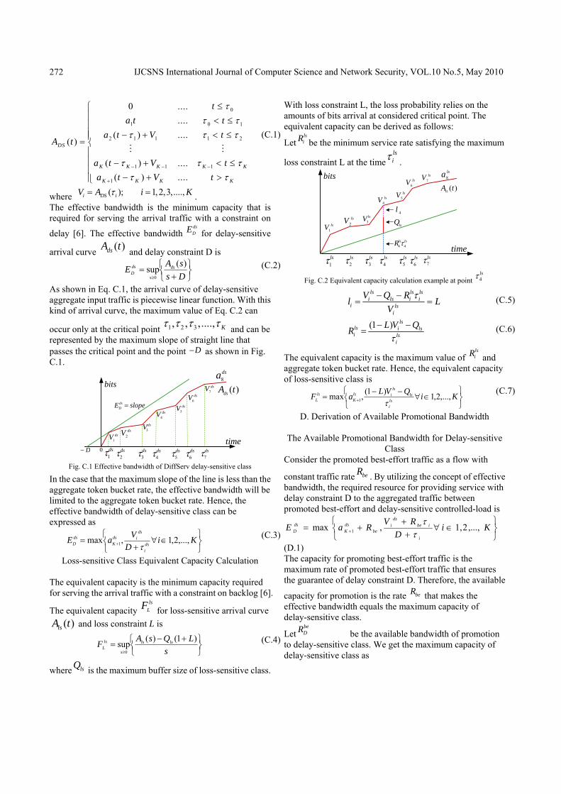
where ( ); 1,2,3,....,i DS iV A i Kτ= = . The effective bandwidth is the minimum capacity that is required for serving the arrival traffic with a constraint on
delay [6]. The effective bandwidth dsDE for delay-sensitive
arrival curve ( )dsA t and delay constraint D is
⎭⎬⎫
⎩⎨⎧
+=
≥ DssAE ds
s
dsD
)(sup0
(C.2)
As shown in Eq. C.1, the arrival curve of delay-sensitive aggregate input traffic is piecewise linear function. With this kind of arrival curve, the maximum value of Eq. C.2 can
occur only at the critical point 1 2 3, , ,...., Kτ τ τ τ and can be represented by the maximum slope of straight line that passes the critical point and the point D− as shown in Fig. C.1.
bits
timedsV1
dsV2
dsV3
dsV4
dsV5
dsV6
dsV7 )(tAds
dsa8
slopeEdsD =
D− ds1τ ds
2τds3τ
ds4τ
ds5τ
ds6τ
ds7τ
0
Fig. C.1 Effective bandwidth of DiffServ delay-sensitive class
In the case that the maximum slope of the line is less than the aggregate token bucket rate, the effective bandwidth will be limited to the aggregate token bucket rate. Hence, the effective bandwidth of delay-sensitive class can be expressed as
⎭⎬⎫
⎩⎨⎧
∈∀+
= + KiD
VaEdsi
dsids
KdsD ,...,2,1,max 1 τ
(C.3)
Loss-sensitive Class Equivalent Capacity Calculation The equivalent capacity is the minimum capacity required for serving the arrival traffic with a constraint on backlog [6].
The equivalent capacity ls
LF for loss-sensitive arrival curve ( )lsA t and loss constraint L is
⎭⎬⎫
⎩⎨⎧ +−
=≥ s
LQsAF lsls
s
lsL
)1()(sup0
(C.4)
where lsQ is the maximum buffer size of loss-sensitive class.
With loss constraint L, the loss probability relies on the amounts of bits arrival at considered critical point. The equivalent capacity can be derived as follows:
LetlsiR be the minimum service rate satisfying the maximum
loss constraint L at the timelsiτ .
bits
time
lsV1
lsV2
lsV3
lsV4
lsV5
lsV6
lsV7
lsa8
)(tAls
ls1τ
ls2τ
ls3τ
ls4τ
ls5τ
ls6τ
ls7τ
4l
lsQ
lslsR 44τ
Fig. C.2 Equivalent capacity calculation example at point 4
lsτ
ls ls lsi ls i i
i lsi
V Q Rl LV
τ− −= = (C.5)
(1 ) lsls i lsi ls
i
L V QRτ
− −= (C.6)
The equivalent capacity is the maximum value of lsiR and
aggregate token bucket rate. Hence, the equivalent capacity of loss-sensitive class is
⎭⎬⎫
⎩⎨⎧
∈∀−−
= + KiQVLaFlsi
lsls
ilsK
lsL ,...,2,1)1(,max 1 τ
(C.7)
D. Derivation of Available Promotional Bandwidth The Available Promotional Bandwidth for Delay-sensitive
Class Consider the promoted best-effort traffic as a flow with
constant traffic rate beR . By utilizing the concept of effective bandwidth, the required resource for providing service with delay constraint D to the aggregated traffic between promoted best-effort and delay-sensitive controlled-load is
⎭⎬⎫
⎩⎨⎧
∈∀++
+= + KiD
RVRaEi
ibeds
ibe
dsK
dsD ,...,2,1,max 1 τ
τ
(D.1) The capacity for promoting best-effort traffic is the maximum rate of promoted best-effort traffic that ensures the guarantee of delay constraint D. Therefore, the available
capacity for promotion is the rate beR that makes the effective bandwidth equals the maximum capacity of delay-sensitive class.
LetbeDR be the available bandwidth of promotion
to delay-sensitive class. We get the maximum capacity of delay-sensitive class as
IJCSNS International Journal of Computer Science and Network Security, VOL.10 No.5, May 2010
273
1max , 1,2, ,
ds beds be i D i
ds K D dsi
V RC a R i KD
ττ+
⎧ ⎫+= + ∀ ∈⎨ ⎬+⎩ ⎭
K (D.2)
Hence, the available bandwidth of promotion is
1
( )min , 1,2, ,ds ds
be ds i ds iD ds K ds
i
D C VR C a i Kττ+
⎧ ⎫+ −= − ∀ ∈⎨ ⎬
⎩ ⎭K
(D.3)
The Available Promotional Bandwidth for Loss-sensitive Class
Similarly, consider the promoted best-effort traffic as a flow
with constant traffic rate beR . By concept of equivalent capacity, the required resource for providing service with loss constraint L to the aggregated traffic between promoted best-effort and loss-sensitive controlled-load is
⎭⎬⎫
⎩⎨⎧
∈∀−+−
+= + KiQRVLRaF lsi
lslsibe
dsi
bedsK
lsL ,...,2,1))(1(,max 1 τ
τ
(D.4) The capacity for promoting best-effort traffic is the maximum rate of promoted best-effort traffic that ensures the guarantee of loss constraint L. Therefore, the available
capacity for promotion is the rate beR that makes the effective bandwidth equals the maximum capacity of loss-sensitive class.
Let beLR be the available bandwidth of promotion to
loss-sensitive class.
1(1 )( )max , 1,2, ,
ls be lsls be i L i ls
ls K L lsi
L V R QC a R i Kττ+
⎧ ⎫− + −= + ∀ ∈⎨ ⎬
⎩ ⎭K (D.5)
Hence, the available bandwidth of promotion is
1(1 )min , 1,2, ,
(1 )
ls lsbe ls ls i ls iL ls K ds
i
C Q L VR C a i KL
ττ+
⎧ ⎫+ − −= − ∀ ∈⎨ ⎬
−⎩ ⎭K (D.6)
Acknowledgements The authors wish to thank Prof. Akinori Nishihara of The Center for Research and Development of Educational Technology, Tokyo Institute of Technology for his support and valuable comments. This work was supported partially by a grant from National Institute of Information and Communication Technology (NICT), Japan. References [1] Armitage, G., “Quality of Service in IP Networks:
Foundations for a Multi-Service Internet,” Macmillan Technical Publishing, Indianapolis, USA, 2000.
[2] Bernet, Y., Ford, P., Yavatkar, R., Baker, F., Zhang, L., Speer, M., Braden, R., Davie, B., Wroclawski, J. and Felstaine, E., “A Framework for Integrated Services Operation over DiffServ Networks”, RFC 2998, IETF, 2000
[3] Blake, S., Black, D., Carlson, M., Davies, E., Wang, Z. and Weiss, W., “An Architecture for Differentiated Services,” RFC 2475, IETF, 1998.
[4] Carpenter, B. E. and Nichols, K., (2002), “Differentiated Services in the Internet,” Proceedings of the IEEE, Vol. 90, No. 9, September, 2002, pp. 1479-1494.
[5] Le Boudec, J. Y. and Thiran, P., “Network Calculus: A Theory of Deterministic Queuing Systems for the Internet,” URL:http://ica1www.epfl.ch/PS_files/NetCal.htm, 2002.
[6] Le Boudec, J.Y.,”Application of Network calculus to Guaranteed service Networks”, IEEE Transactions on Information Theory, Vol.11, No.3, May1998, pp.1087-1096.
[7] Matrawy, A., Lambadaris I. and Huang C., “MPEG4 Traffic Modeling using The Transform Expand Sample Methodology,” Proceedings of the 4th IEEE International Workshop on Networked Appliances (IWNA4), Gaithersburg, USA, January, 2002.
[8] Parekh, A. K. and Gallager, R. G., “A Generalized Processor Sharing Approach to Flow Control in Integrated Services Networks: The Single-Node Case,” IEEE/ACM Transactions on Networking, Vol. 1, No. 3, June, 1993, pp. 344-357.
[9] Shenker, S., Partridge, C. and Guerin, R., “Specification of Guaranteed Quality of Service”, RFC 2212 IETF.
[10] Urwijitaroon R., “QoS Provisioning Strategy for QoS-Unaware Applications in an IntServ/DiffServ Interoperating Network” M.Eng. Thesis, Telecommunications Program, School of Advanced Technologies, Asian Institute of Technology, Pathumthani, Thailand, 2003.
[11] Thomas, A., “Supplying Legacy Applications with QoS: A Description Syntax at Application, End-user and Network Level,” IASTED International Conference on Software Engineering and Applications (SEA2002), Cambridge, USA, November, 2002.
[12] Wroclawski, J., “Specification of the Controlled-Load Network Element Service”, RFC 2211, IETF.
[13] NS-2 http://www.isi.edu/nsnam/ns
Teerapat Sanguankotchakorn was born in Bangkok Thailand on 08th December 1965. He received the B.Eng in Electrical Engineering from Chulalongkorn University, Thailand in 1987, M.Eng and D.Eng in Information Processing from Tokyo Institute of Technology, Japan in 1990 and 1993, respectively under Japanese Government Scholarship. In 1993, he joined
Telecommunication and Information Systems Research Laboratory at Sony Corporation, Japan, where he holds two patents on Signal Compression. He joined Asian Institute of Technology in October 1998 as an Assistant Professor. Currently, he is an Associate Professor at Telecommunications Field of Study, School of Engineering and Technology, Asian Institute of Technology. His research interests include Digital Signal Processing, High Speed Network, IP-based multimedia applications and QoS in IP and Mobile Ad Hoc Network. He is the senior member of IEEE and member of IEICE, Japan
Ruenun Urwijitaroon was born in Bangkok Thailand. He received the B.Eng in Electrical Engineering from Chulalongkorn University, Thailand in 2001 and M.Eng in Telecommunication from Telecommunications field of Study, School of Engineering and Technology, Asian Institute of Technology, Thailand in 2003. Currently, he is working at Huawei
Technologies (Thailand) Co., Ltd. in Thailand. His major fields of research are High Speed Network and Quality of Service in IP Network.