qos measurement and management for multimedia services thesis proposal wenyu jiang april 29, 2002
Post on 20-Dec-2015
222 views
TRANSCRIPT

QoS Measurement and Management QoS Measurement and Management for Multimedia Servicesfor Multimedia Services
Thesis Proposal
Wenyu Jiang
April 29, 2002

Topics CoveredTopics CoveredObjective QoS metrics for real-time
multimediaSubjective/Perceived qualityObjective perceptual quality
estimation algorithmsQuality enhancement for real-time
multimediaIP telephony deploymentVoIP quality in the current Internet

Backgrounds and MotivationsBackgrounds and Motivations
The Internet is still best-effort– Needs QoS monitoring
What to measure/monitor?– Loss, delay, jitter– Must map to perceived quality
What to do if quality is not good?– End-to-End: FEC, LBR– Network provisioning: voice traffic aggregation
IP telephony service deployment– Current ITSPs are not doing well– Lack of study on localized deployment
What is the status of the current Internet?

How Real-time Multimedia WorksHow Real-time Multimedia Works
A/D conversion; Encoding; Packet transmission; Decoding; Playout; D/A conversion
Dominant QoS factors:– Loss clipping/distortion in audio– Delay lower interactivity– Jitter late loss
new
delayplayout
late lossesadded more
Sender
unrecovered
ment
signalrecovery
repairedcompressedmedia
delayReceiver
mediasignal
packets with
control
lossesInternetcoder FEC
redundant
delay
playout
FECdecodedmediapackets with loss
packets
playout lossconceal- decoder

Delay and Loss MeasurementDelay and Loss Measurement
Solutions for clock synchronization– Telephone-based synchronization– RTT-based, assume symmetric delays– GPS-based
Dealing with Clock drift– De-skewing by linear regression
One-way vs. round-trip measurement– Internet load often asymmetric– One-way loss and delay are more
relevant to real-time multimedia

Loss and Delay ModelsLoss and Delay Models
Loss Models– Gilbert model– Extended Gilbert model– Others
Delay Models– More difficult to construct– No universal distribution function– Temporal correlation between delays
0 11-p p
q
(non-loss) (loss)
1-q = p c
00p = 1 - p
01
= 1 - p2320
p
10p = 1 - p
12
0S 2S
p12
n-1S(n-2)(n-1)pp
01
1S1 consecutive
loss. . .
losses losses
p(n-1)(n-1) = 0
p(n-1)0
= 1 - p(n-1)(n-1)
= 1
(non-loss)2 consecutive n-1 consecutive

Perceived Quality EstimationPerceived Quality Estimation
Mean Opinion Score (MOS)– Requires human listeners– Labor and time intensive– Reflective of real quality
Objective perceptual quality estimation algorithms– PESQ, PSQM/PSQM+, MNB, EMBSD– Speech recognition based (new)
MOS Grade Score
Excellent 5
Good 4
Fair 3
Poor 2
Bad 1

Network Provisioning for VoIPNetwork Provisioning for VoIP
Silence suppression– Saves bandwidthstatistical multiplexing– The on/off patterns in human voice depend
on the voice codec or the silence detectorVoice traffic aggregation
– Multiplexing by token bucket filtering– The on/off patterns in human voice directly
affects aggregation performance• Past study assumes exponential distribution

IP Telephony DeploymentIP Telephony DeploymentLocalized deployment
– More practical than a grand-scale Internet deployment
– Can still interoperate with an IP telephony carrier
Issues– PSTN interoperability– Security– Scalability– Billing

Research ObjectivesResearch Objectives
Objective QoS metrics– Modeling– Their relationship to perceived quality
Objective perceptual quality estimation algorithms vs. perceived quality (MOS)
Quality improvement measures– End-to-End: FEC vs. LBR– Network-based: voice traffic aggregation
IP telephony deployment issues VoIP quality measurement over the Internet

Completed Work: QoS Completed Work: QoS Measurement ToolsMeasurement Tools
UDP packet trace generator Clock synchronization and de-skewing tool Loss and delay modeling tools
– By examining a packet trace– Outputs Gilbert and extended Gilbert model
parameters– Outputs conditional delay CCDF
Playout simulator– Simulates several common playout algorithms– FEC is also supported

Completed Work: Comparison of Completed Work: Comparison of Loss ModelsLoss Models Loss burst distribution
– Roughly, but not exactly exponential Inter-loss distance
– Clustering between adjacent loss bursts
0
1
10
100
1000
0 2 4 6 8 10 12
num
ber
of o
ccur
renc
es
Loss burst length
Packet traceGilbert model

Loss Model Comparison, contd.Loss Model Comparison, contd.
Loss burstiness on FEC performance– FEC less efficient under bursty loss
Final loss pattern (after playout, FEC)– Generally also bursty
0
0.5
1
1.5
2
2.5
3
10 20 30 40 50 60
p_f:
fina
l los
s% a
fter
FE
C
conditional loss p_c (%)
GilbertBernoulli
0
1
10
100
1000
1 1.5 2 2.5 3 3.5 4 4.5 5
num
ber
of o
ccur
renc
es
Loss burst length
Example Final Loss Pattern after Playout
Exp-AvgPrev-Opt

Mapping from Loss Model to Mapping from Loss Model to Perceived QualityPerceived Quality
Random vs. bursty loss– Bursty lower MOS
Effect of loss burstiness– Sometimes very bursty
loss does not lead to lower quality 2
2.5
3
3.5
4
4.5
0.02 0.04 0.06 0.08 0.1 0.12
MO
S
loss probability
Effect of random vs. bursty loss on MOS quality
random (Bernoulli) lossbursty (Gilbert) loss
2
2.5
3
3.5
4
0.04 0.08 0.12 0.16
MO
S
p_u (average loss probability)
T=20ms fixed, p_c=30-50%
p_c=30%p_c=50%
2
2.5
3
3.5
4
0.04 0.08 0.12 0.16
MO
S
p_u (average loss probability)
T=40ms fixed, p_c=30-50%
p_c=30%p_c=50%

A New Delay ModelA New Delay Model
Conditional CCDF (C3DF)Allows estimation of burstiness in
the late losses introduced by (fixed) playout algorithm
lag=3
lag=5
lag=10lag=20
unconditional
lag=2
lag=1
0
0.2
0.4
0.6
0.8
1
0 0.05 0.1 0.15 0.2 0.25 0.3
y: p
roba
bilit
y
x: delay (sec)
id
l
tdtdPtf
i
lii
packet ofdelay :
,...3,2,1 lag
]|[)(

Objective vs. Subjective MOSObjective vs. Subjective MOS
Algorithms: PESQ, PSQM, PSQM+, MNB, EMBSD
1
1.5
2
2.5
3
3.5
4
4.5
1.5 2 2.5 3 3.5 4 4.5
Obj
ectiv
e M
OS
Subjective MOS
Objective MOS correlation
MNB1MNB2PESQ
1
1.5
2
2.5
3
3.5
4
4.5
1.5 2 2.5 3 3.5 4 4.5
Obj
ectiv
e M
OS
Subjective MOS
Objective MOS correlation
MNB1MNB2PESQ
Using Original Linear 16 samples as reference signal
Using G.729 no loss clip as reference signal

Objective MOS Correlation, contd.Objective MOS Correlation, contd.
Second test set Stronger “saturation” effect observed for
MNB1 and MNB2, but not for PESQ
2
2.5
3
3.5
4
4.5
2 2.5 3 3.5 4 4.5
Obj
ectiv
e M
OS
Subjective MOS
Objective MOS correlation
MNB1MNB2PESQ
2
2.5
3
3.5
4
4.5
2 2.5 3 3.5 4 4.5
Obj
ectiv
e M
OS
Subjective MOS
Objective MOS correlation
MNB1MNB2PESQ
Linear-16 reference signal G.729 reference signal

Auditory Distance vs. MOSAuditory Distance vs. MOS
EMBSD and PSQM+ appear to have the largest spread, i.e., least correlation w. MOS
PSQM seems to be similar to MNB in terms of correlation
0
1
2
3
4
5
6
7
1.5 2 2.5 3 3.5 4 4.5
Obj
ectiv
e P
erce
ptua
l Dis
tanc
e
Subjective MOS
Objective vs. subjective quality correlation
EMBSDPSQM
PSQM+MNB1MNB2
0
1
2
3
4
5
6
7
1.5 2 2.5 3 3.5 4 4.5
Obj
ectiv
e P
erce
ptua
l Dis
tanc
e
Subjective MOS
Objective vs. subjective quality correlation
EMBSDPSQM
PSQM+MNB1MNB2

Auditory Distance vs. MOS, contd.Auditory Distance vs. MOS, contd.
Second test setSimilar behaviors observed
0
1
2
3
4
5
6
7
2 2.5 3 3.5 4 4.5
Obj
ectiv
e P
erce
ptua
l Dis
tanc
e
Subjective MOS
Objective vs. subjective quality correlation
EMBSDPSQM
PSQM+MNB1MNB2
0
1
2
3
4
5
6
7
2 2.5 3 3.5 4 4.5
Obj
ectiv
e P
erce
ptua
l Dis
tanc
e
Subjective MOS
Objective vs. subjective quality correlation
EMBSDPSQM
PSQM+MNB1MNB2
Linear-16 reference signal G.729 reference signal

Analysis of Objective MOS Analysis of Objective MOS CorrelationCorrelationQuantitative metric
– Correlation coefficient – But it does not tell everything!
Algorithm Test Set 1 Test Set 2
l16 g729 l16 g729
MNB1 0.897 0.885 0.767 0.798
MNB2 0.910 0.935 0.844 0.870
PESQ 0.888 0.902 0.892 0.910

Speech Recognition Performance Speech Recognition Performance as a MOS predictoras a MOS predictor
Evaluation of automatic speech recognition (ASR) based MOS prediction– IBM ViaVoice Linux version– Codec used: G.729– Performance metric
• absolute word recognition ratio
• relative word recognition ratiodsspoken wor of # total
wordsrecognizedcorrectly of #absR
yprobabilit loss is ,%)0(
)()( p
R
pRpR
abs
absrel

Recognition Ratio vs. MOSRecognition Ratio vs. MOS
Both MOS and Rabs decrease w.r.t loss
Then, eliminate middle variable p
2
2.2
2.4
2.6
2.8
3
3.2
3.4
3.6
3.8
28 30 32 34 36 38 40 42 44
MO
S
word recognition ratio (%)
mapping from speech recognition performance to MOS
speech recognition performance
2
2.2
2.4
2.6
2.8
3
3.2
3.4
3.6
0 2 4 6 8 10 12 14 16
MO
S
loss rate (%)
Impact of packet loss on audio quality
G.729 codec
28
30
32
34
36
38
40
42
44
0 2 4 6 8 10 12 14 16
wor
d re
cogn
ition
rat
io (%
)
loss rate (%)
Impact of packet loss on automatic speech recognition
G.729 codec

Speaker Dependency CheckSpeaker Dependency Check
Absolute performance is speaker-dependent
But relative word recognition ratio is not
25
30
35
40
45
50
55
60
65
70
75
0 2 4 6 8 10 12 14 16
wor
d re
cogn
ition
rat
io (%
)
loss rate (%)
Impact of packet loss on machine speech recognition
Speaker ASpeaker B
65
70
75
80
85
90
95
100
0 2 4 6 8 10 12 14 16rela
tive
wor
d re
cogn
ition
rat
io R
_rel
(%)
loss rate (%)
Impact of packet loss on machine speech recognition
Speaker ASpeaker B
2
2.2
2.4
2.6
2.8
3
3.2
3.4
3.6
3.8
65 70 75 80 85 90 95 100
MO
S
relative word recognition ratio R_rel (%)
speaker A, trained by G.729speaker B, trained by G.729

Speech Intelligibility ResultsSpeech Intelligibility Results
Human listeners are asked to do transcription
Human recognition result curves are less “smooth” than MOS curves.
50
55
60
65
70
75
80
85
0 2 4 6 8 10 12 14 16
abso
lute
wor
d re
cogn
ition
rat
io (%
)
loss rate (%)
Impact of packet loss on human speech recognition
Human recognition performance
2
2.2
2.4
2.6
2.8
3
3.2
3.4
3.6
3.8
50 55 60 65 70 75 80 85
MO
S
absolute word recognition ratio R_abs (%)
mapping from human recognition performance to MOS
human recognition performance
50
55
60
65
70
75
80
85
90
28 30 32 34 36 38 40 42 44
Hum
an R
_abs
(%)
Machine R_abs (%)
human vs. machine recognition performance
human recognition performance

Analysis of Voice On-Off PatternsAnalysis of Voice On-Off Patterns Past study finds spurt &
gap distributions to be exponential
Modern voice codecs and silence detectors have different behaviors 1e-05
0.0001
0.001
0.01
0.1
1
0 50 100 150 200 250 300 350 400 450 500
com
plem
enta
ry C
DF
spurt/gap duration (in 10 ms frames)
talk-spurt/gap distribution, G.729B VAD
real spurt CDFexponential spurt CDF
real gap CDFexponential gap CDF
1e-05
0.0001
0.001
0.01
0.1
1
0 50 100 150 200 250 300 350 400 450 500
com
plem
enta
ry C
DF
spurt/gap duration (in 10 ms frames)
talk-spurt/gap distribution, Nevot SD (low threshold, short hangover)
real spurt CDFexponential spurt CDF
real gap CDFexponential gap CDF
1e-05
0.0001
0.001
0.01
0.1
1
0 200 400 600 800 1000
com
plem
enta
ry C
DF
spurt/gap duration (in 10 ms frames)
talk-spurt/gap distribution, Nevot SD (default setting)
real spurt CDFexponential spurt CDF
real gap CDFexponential gap CDF

Voice Traffic AggregationVoice Traffic Aggregation
Simulation environment– DiffServ token bucket filter– Exponential, CDF and trace-
based model simulations– N voice sources– Token buffer size B (packets)– R: ratio of reserved vs. peak
bandwidth
Key performance figure– Probability of out-of-profile
packet
tokens
sourcesN voice
FillingToken
data drain
cursor N
cursor 2
cursor 1
cursor 3
silence detector traceas circular buffer

Aggregation Simulation ResultsAggregation Simulation Results
Results based on G.729 VAD– CDF model resembles trace model in most cases– Exponential (traditional) model
• Under-predicts out-of-profile packet probability;• The under-prediction ratio increases as token buffer size B increases
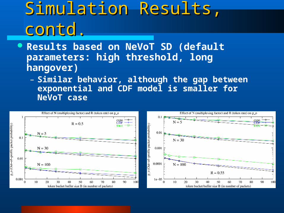
Simulation Results, contd.Simulation Results, contd.
Results based on NeVoT SD (default parameters: high threshold, long hangover)– Similar behavior, although the gap between
exponential and CDF model is smaller for NeVoT case

Comparisons of FEC and LBRComparisons of FEC and LBR
Forward error correction– Bit-exact recovery– No decoder state drift upon recovery
Low bit-rate redundancy (LBR)– Just the opposite to FEC
Design of an optimal LBR algorithm– State repair via redundant codec– Optimal packet alignment– MOS quality verified to be better than the rat LBR– Allows a more “fair” comparison with FEC

MOS Quality of FEC vs. LBR MOS Quality of FEC vs. LBR
FEC shows a substantial and consistent advantage over LBR– This is true for all LBR configurations we tested
Main codec is G.729 except for AMR LBR
2
2.5
3
3.5
4
4.5
0.02 0.04 0.06 0.08 0.1 0.12
MO
S
loss probability
FEC vs. LBR based on DoD-LPC
D: FEC (4,3)C: DoD-LPC LBR
2
2.5
3
3.5
4
4.5
0.02 0.04 0.06 0.08 0.1 0.12
MO
S
loss probability
FEC vs. LBR based on DoD-CELP
F: FEC (3,2)E: DoD-CELP LBR
DoD-LPC LBR DoD-CELP LBR

MOS of FEC vs. LBR, contd.MOS of FEC vs. LBR, contd.
AMR LBR: narrowest gap with FEC (Not shown here) FEC out-performs LBR
under random loss as well
2
2.5
3
3.5
4
4.5
0.02 0.04 0.06 0.08 0.1 0.12
MO
S
loss probability
FEC vs. LBR based on G.723.1
J: FEC (2,1)I: G.723.1 LBR
2
2.5
3
3.5
4
4.5
0.02 0.04 0.06 0.08 0.1 0.12
MO
S
loss probability
FEC vs. LBR based on AMR
N: AMR12.2+FEC (3,2)M: AMR12.2+6.7 LBR
G.723.1 LBR AMR LBR

Optimizing FEC QualityOptimizing FEC Quality
Packet interval loss burstiness FEC efficiency
Result: FEC MOS performance also improves
0.5-0.6 MOS
2.5
3
3.5
4
4.5
0.02 0.04 0.06 0.08 0.1 0.12 0.14 0.16 0.18
MO
S (M
ean
Opi
nion
Sco
re)
p_u (overall loss rate)
conditional loss probability p_c = 30%
T=20ms
2
T=40ms
T=20ms, FEC
T=40ms, FEC
0
5
10
15
20
25
30
35
40
45
50
20 30 40 50 60 70 80
obse
rved
p_c
(%)
packet interval T (ms)
p_c = 50% @ T=20msp_c = 30% @ T=20ms
Bernoulli

Optimizing Conversational MOS Optimizing Conversational MOS for FECfor FEC
A larger packet interval more delay Trade-off between quality and delay The E-model
– Considers both delay and loss (and many other transmission quality factors)
Optimizing FEC MOS with the E-model
2.4
2.6
2.8
3
3.2
3.4
3.6
3.8
4
4.2
20 40 60 80 100 120 140 160 180
MO
S_c
packet interval T (ms)
Effect of delay impairment Id on FEC MOS
FEC MOS if Id = 0FEC MOS if Id != 0 (d=3*T)
FEC MOS under Bernoulli loss
2
2.5
3
3.5
4
20 40 60 80 100 120 140 160 180
MO
S_c
packet interval T (ms)
FEC MOS optimization, Id != 0, d=3*T
p_u=4%p_u=8%
p_u=12%p_u=16%

Optimizing FEC MOS, contd.Optimizing FEC MOS, contd.
Validating E-model based prediction with real MOS test results
2.4
2.6
2.8
3
3.2
3.4
3.6
3.8
4
4.2
0 2 4 6 8 10 12 14 16
MO
S_c
original loss rate (%)
FEC MOS prediction, p_c=30%
E-model prediction T=40msreal MOS test T=40ms

Localized IP Telephony Localized IP Telephony Deployment: ArchitectureDeployment: Architecture
Component based and distributed architecture
Allows easy integration of all SIP-compliant devices and programs

Deployment IssuesDeployment Issues
PSTN interoperability– T1 configuration and PBX integration
• T1 line type (Channelized vs. ISDN PRI)• Line coding and framing (layer 2)• Trunk type: Direct-inward-dialing (DID)• Access permission on the PBX side
– SIP/PSTN gateway configuration• Dial-peer: locates the proper SIP server or
PSTN trunk• Dial-plan (translating calls from/to PSTN)

Deployment Issues, contd.Deployment Issues, contd. Security
– Issue: gateway has no authentication feature– Solution:
• Use gateway’s access control lists to block direct calls• SIP proxy server handles authentication using record-route
– Allows easier change in authentication module (software-based)
– Certain users can only make certain gateway calls Scalability
– SIP server (DNS SRV scaling)– Gateway; voice-mail server; conference server
Billing– Initial implementation via transaction logging

On-going ResearchOn-going Research
Measurement of the current InternetHow well can it support VoIP?
– Or, how easy can VoIP applications adapt to (unfavorable) network conditions?
• How fast does network condition change?
Can network redundancy help improve VoIP quality?– Physical redundancy (access links)– Virtual redundancy (overlay networking)

ConclusionsConclusions
Completed research relating to many aspects of real-time multimedia, in particular VoIP
On-going work calls for:– A comprehensive measurement of the
Internet– Analysis of the to-be measurement data– An answer to the question: how good is
it today, and, how much better can we do?