qos aware packet scheduling in the downlink of …yue/thesis/rehana kausar.pdf · 1 abstract this...
TRANSCRIPT

QoS Aware Packet Scheduling in the Downlink of LTE-Advanced Networks
Rehana Kausar
Submitted for the Degree of Doctor of Philosophy
School of Electronic Engineering & Computer Science Queen Mary University of London
January 2013

To my parents
1
Abstract
This thesis considers QoS aware packet scheduling in the downlink of LTE-Advanced
networks. The outcome of this research is improved QoS performance for real-time services
while maintaining the overall system-level performance.
A QoS aware scheduling architecture is proposed that extends the traditional MAC layer
scheduling into a three-stage cross-layer architecture that takes information from the
Physical, MAC and application layers. The system includes:
two service-specific queue-sorting algorithms for both real-time and non-real time
service in the traffic differentiating stage to prioritise users;
an adaptive scheduling algorithm in the time-domain scheduling stage that
incorporates machine learning to achieve adaptive resource allocation; and
a frequency domain scheduling stage using a modified proportional fairness
algorithm for resource allocation.
The first two stages are completely novel, as is the combination with the frequency domain
scheduling which uses modified proportional fairness algorithm.
The performance of the proposed algorithms is evaluated in a system-level simulator under
different network scenarios. Simulation results show that the approach can (i) reduce the
average delay of the real-time service and fulfil the minimum throughput requirements of
the non-real time service and (ii) achieve a good trade-off between user-level and system-
level performance.

2
Acknowledgements
All praises and thankfulness is for Allah the Almighty who gave me the courage,
determination and steadfastness to complete this thesis. I would like to present my humble
thanks to my great religious leader for his precious prayers and also for his financial support
during my study, may Allah give him the best reward.
I would like to take this opportunity to express my sincere gratitude to my supervisor, Dr
Yue Chen, for her invalueable academic support. Her supervision, apart from academics,
groomed me logically and always guided me towards positive and progressive thinking.
Her advice has always been the greatest source of motivation for me. Also I would like to
thank Dr Michael Chai for his continous support and encouragement at every stage of my
study. I would like to thank Prof Laurie Cuthbert, Dr John Schormans, Dr Silvano P V Barros
(late) and Dr Vindya Wijeratne for their help and support.
I wish to extend my gratitude to all the support staff of the department, who have made the
technical part of my work possible. Many thanks to my colleagues and friends who have
encouraged and advised me and made my time here memorable.
Finally, I would like to thank my husband Mansoor Ahmed and my family for their love,
continous prayers and enourmous support. They always be my strongest power to work
hard and get through hard times. With all my love and gratitude, I want to dedicate this
thesis to my father Jamil Ahmad Tahir (late) who had a great wish to see me as doctor and to
my mother Amtul Hai for her continuous prayers.

3
Declaration
I hereby declare that the work presented in this thesis is solely my work and that to
the best of my knowledge the work is original except where indicated by reference to
the respective authors.
Rehana Kausar
Date:

4
Table of Contents
To my parents ....................................................................................................................................... 1
Abstract.................................................................................................................................................. 2
Acknowledgements ............................................................................................................................. 2
Declaration ............................................................................................................................................ 3
List of Figures ....................................................................................................................................... 7
List of Tables ....................................................................................................................................... 10
List of Abbreviations ......................................................................................................................... 11
Chapter 1 Introduction ................................................................................................................ 14
Background and Motivation ............................................................................................. 14 1.1
Research Scope ................................................................................................................... 15 1.2
Contributions ...................................................................................................................... 16 1.3
Author’s Publication .......................................................................................................... 18 1.4
Thesis Organisation ........................................................................................................... 19 1.5
Chapter 2 Research Study ........................................................................................................... 21
Access Technologies in Wireless Mobile Networks ...................................................... 21 2.1
OFDMA in Long Term Evolution (LTE) Networks ...................................................... 24 2.2
Packet Scheduling .............................................................................................................. 28 2.3
Scheduling in LTE-A Networks ....................................................................................... 30 2.4
QoS Classes and QoS Requirements ............................................................................... 32 2.5
Classic Packet Scheduling Algorithms ............................................................................ 39 2.6
Round Robin (RR) Algorithm................................................................................... 39 2.6.1
Maximum Carrier to Interference (MAX C/I) Algorithm .................................... 41 2.6.2
Proportional Fairness (PF) Algorithm ..................................................................... 42 2.6.3
Generalised Proportional Fairness Algorithm ............................................................... 44 2.7
QoS Aware Packet Scheduling Algorithms .................................................................... 44 2.8
Quality of Service (QoS) and Queue State Information (QSI) ............................. 45 2.8.1
Modified Largest Weighted Delay First (MLWDF) .............................................. 46 2.8.2
Subcarrier Allocation for OFDMA Systems ........................................................... 47 2.8.3
Sum Waiting Time Based Scheduling (SWBS) ....................................................... 47 2.8.4
Mixed Traffic Packet Scheduling in UTRAN (MIX) .............................................. 48 2.8.5
Machine Learning in Scheduling ..................................................................................... 49 2.9
5
Hebbian Learning ...................................................................................................... 50 2.9.1
Clustering .................................................................................................................... 51 2.9.2
Problem Description .......................................................................................................... 52 2.10
Summary ............................................................................................................................. 54 2.11
Chapter 3 Cross-Layer Design for QoS Aware Scheduling Architecture ............................ 55
Principle of Design of Scheduling Architecture ............................................................ 55 3.1
Traffic Differentiator .................................................................................................. 56 3.1.1
TD Scheduler .............................................................................................................. 57 3.1.2
FD Scheduler ............................................................................................................... 57 3.1.3
Cross-Layer Concept ................................................................................................. 58 3.1.4
System Model ..................................................................................................................... 59 3.2
Queue Sorting Algorithms in Traffic Differentiator ..................................................... 62 3.3
FCFS Algorithm for Control Traffic Queue ............................................................ 63 3.3.1
Novel Queue Sorting Algorithm for RT Queue ..................................................... 65 3.3.2
Novel Queue Sorting Algorithm for NRT Queue ................................................. 68 3.3.3
PF Algorithm for BE Queue ...................................................................................... 71 3.3.4
Machine Learning Algorithms in TD Scheduler............................................................ 72 3.4
Hebbian learning Process in ATDSA ...................................................................... 73 3.4.1
K-Mean Clustering Algorithm in ATDSA .............................................................. 81 3.4.2
Modified PF Algorithm in FD Scheduler ........................................................................ 84 3.5
System-Level Performance Indicators............................................................................. 85 3.6
Summary ............................................................................................................................. 86 3.7
Chapter 4 System Level Platform ............................................................................................... 87
Design of System Level Simulation Platform ................................................................ 87 4.1
Simulation Flow ................................................................................................................. 89 4.2
Module Functionality and Implementation ................................................................... 92 4.3
Initialisation Module ................................................................................................. 92 4.3.1
Traffic Differentiating Module ................................................................................. 92 4.3.2
Adaptive TD Scheduling Module ............................................................................ 93 4.3.3
Resource Allocation Module .................................................................................... 95 4.3.4
Feedback Module ....................................................................................................... 95 4.3.5
Wireless Channel Model ................................................................................................... 96 4.4
Path Loss Model ......................................................................................................... 98 4.4.1
Shadow Fading Model ............................................................................................ 101 4.4.2
Multipath Fading ..................................................................................................... 101 4.4.3

6
Radio Resource Allocation .............................................................................................. 102 4.5
Simulation Validation ...................................................................................................... 103 4.6
Random Distribution of UEs .................................................................................. 104 4.6.1
Verification of the Proposed Architecture ............................................................ 105 4.6.2
Verification of the Number of Iterations ............................................................... 108 4.6.3
Summary ........................................................................................................................... 110 4.7
Chapter 5 Simulation Results and Analysis ........................................................................... 111
Traffic Model .................................................................................................................... 112 5.1
User Queuing Model ....................................................................................................... 114 5.2
Performance Evaluation of SSSA ................................................................................... 114 5.3
QoS Performance of Real Time and Streaming Services .................................... 115 5.3.1
System Performance ................................................................................................ 121 5.3.2
Joint (SSSA & ATDSA) Performance Evaluation ......................................................... 123 5.4
Scenario 1: Equal Distribution of Real Time and Non Real time Services ....... 125 5.4.1
Scenario 2: Real Time Service Dominant over Other Services ........................... 131 5.4.2
Scenario 3: Background Service Dominant over Other Services ....................... 137 5.4.3
Scenario 4: Streaming Service Dominant over Other Services .......................... 143 5.4.4
Performance Analysis of CLPSA ........................................................................... 149 5.4.5
Performance Evaluation of K-Mean Clustering Algorithm ....................................... 155 5.5
Summary ........................................................................................................................... 157 5.6
Chapter 6 Conclusions and Future Work ............................................................................... 158
Conclusions ....................................................................................................................... 158 6.1
Future Work ...................................................................................................................... 160 6.2
References ......................................................................................................................................... 161
7
List of Figures
Figure 2-1 Evolution of access technologies in mobile cellular networks .................................. 21
Figure 2-2 FDMA and TDMA technology ...................................................................................... 23
Figure 2-3 CDMA multiple access technology in 3G networks................................................... 24
Figure 2-4 OFDMA technology ........................................................................................................ 25
Figure 2-5 The OFDMA technology in LTE/LTE-A ..................................................................... 27
Figure 2-6 Basic model of a packet scheduler ................................................................................ 28
Figure 2-7 Reference signals ............................................................................................................. 31
Figure 2-8 QoS framework of LTE network ................................................................................... 38
Figure 2-9 Round Robin (RR) algorithm ......................................................................................... 40
Figure 2-10 Maximum Carrier to Interference (MAX C/I) algorithm ........................................ 41
Figure 2-11 Proportional Fairness (PF) algorithm ......................................................................... 43
Figure 3-1 Cross-layer QoS aware packet scheduling architecture ............................................ 55
Figure 3-2 Cross-layer design for QoS aware scheduling architecture ...................................... 58
Figure 3-3 Downlink transmission .................................................................................................. 59
Figure 3-4 Traffic differentiator Stage ............................................................................................. 62
Figure 3-5 PDCCH resource allocation from PCFICH ................................................................. 64
Figure 3-6 A system with two UEs .................................................................................................. 67
Figure 3-7 TD scheduler stage .......................................................................................................... 73
Figure 3-8 Hebbian learning process ............................................................................................... 76
Figure 3-9 K-Mean clustering algorithm......................................................................................... 83
Figure 4-1 Flow chart of simulation platform ................................................................................ 91
Figure 4-2 Flow chart of initial module .......................................................................................... 92
Figure 4-3 Flow chart of traffic differentiating module ................................................................ 93
Figure 4-4(a) Flow chart of Hebbian learning module ................................................................. 94
Figure 4-4(b) Flow chart of K-mean clustering module ............................................................... 94
Figure 4-5 Flow chart of resource allocation module ................................................................... 95
Figure 4-6 Flow chart of feedback module ..................................................................................... 96
Figure 4-7 Radio channel attenuation ............................................................................................. 97
Figure 4-8 Transmission characteristics of a signal in wireless channel .................................... 98
Figure 4-9 Parameters for computation .......................................................................................... 98
Figure 4-10 UE positions when UE number is 50 ........................................................................ 104
8
Figure 4-11 System throughput for 20 users ................................................................................ 106
Figure 4-12 System throughput for different number of active users ...................................... 107
Figure 4-13 System instantaneous throughput ............................................................................ 108
Figure 4-14 System average throughput vs. number of loops ................................................... 109
Figure 5-1 ON-OFF traffic model ................................................................................................... 113
Figure 5-2 A user’s queue model ................................................................................................... 114
Figure 5-3 System model of SSSA .................................................................................................. 115
Figure 5-4 Average delay of real-time service ............................................................................. 116
Figure 5-5 Packet drop rate of real-time service .......................................................................... 117
Figure 5-6 Standard deviation of average PDR distribution of RT users................................. 118
Figure 5-7 Average achieved throughput of streaming service ................................................ 119
Figure 5-8 Average throughput of background service ............................................................. 120
Figure 5-9 Fairness among all users .............................................................................................. 121
Figure 5-10 System spectral efficiency .......................................................................................... 122
Figure 5-11 System model of CLPSA ............................................................................................ 124
Figure 5-12 Average packet delay of real-time service ............................................................... 125
Figure 5-13 Average PDR of real-time service ............................................................................. 126
Figure 5-14 Standard deviation of average PDR of RT users .................................................... 127
Figure 5-15 Average achieved throughput of streaming service .............................................. 128
Figure 5-16 Fairness among all users ............................................................................................ 129
Figure 5-17 System throughput...................................................................................................... 130
Figure 5-18 Average packet delay of real-time service ............................................................... 131
Figure 5-19 Average PDR of real-time service ............................................................................. 132
Figure 5-20 Standard deviation of average PDR distribution of all RT users ......................... 133
Figure 5-21 Average achieved throughput of streaming service .............................................. 134
Figure 5-22 Fairness among all users ............................................................................................ 135
Figure 5-23 System throughput...................................................................................................... 136
Figure 5-24 Average packet delay of real-time service ............................................................... 137
Figure 5-25 Average PDR of real-time service ............................................................................. 138
Figure 5-26 Standard deviation of average PDR distribution of all RT users ......................... 139
Figure 5-27 The average achieved throughput of streaming traffic ......................................... 140
Figure 5-28 Fairness among all users ............................................................................................ 141
Figure 5-29 System throughput...................................................................................................... 142
Figure 5-30 Average packet delay of real-time service ............................................................... 143

9
Figure 5-31 Average PDR of real-time service ............................................................................. 144
Figure 5-32 Standard deviation of average PDR distribution of RT users ............................... 145
Figure 5-33 Average achieved throughput of streaming traffic ................................................ 146
Figure 5-34 Fairness among all users ............................................................................................ 147
Figure 5-35 System spectral efficiency .......................................................................................... 148
Figure 5-36 Average packet delay of real-time service ............................................................... 149
Figure 5-37 Average packet drop rate of real-time service ........................................................ 150
Figure 5-38 Standard deviation of average PDR distribution of RT users ............................... 151
Figure 5-39 Average achieved throughput of streaming traffic ................................................ 152
Figure 5-40 Fairness among all users ............................................................................................ 153
Figure 5-41 Standard deviation of average PDR distribution of RT users ............................... 155
Figure 5-42 Average packet drop rate of real-time service ........................................................ 156
10
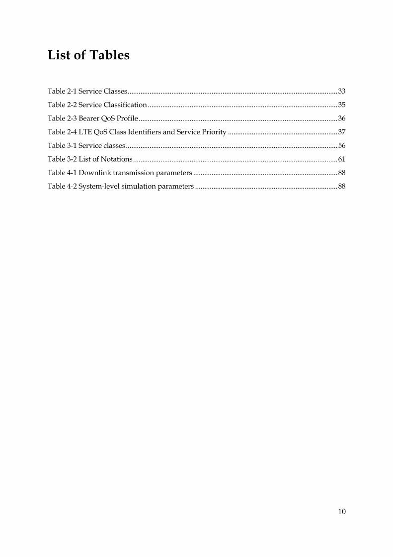
List of Tables
Table 2-1 Service Classes ................................................................................................................... 33
Table 2-2 Service Classification ........................................................................................................ 35
Table 2-3 Bearer QoS Profile ............................................................................................................. 36
Table 2-4 LTE QoS Class Identifiers and Service Priority ............................................................ 37
Table 3-1 Service classes .................................................................................................................... 56
Table 3-2 List of Notations ................................................................................................................ 61
Table 4-1 Downlink transmission parameters ............................................................................... 88
Table 4-2 System-level simulation parameters .............................................................................. 88

11
List of Abbreviations
1G First Generation
2G Second Generation
3G Third Generation
4G Fourth Generation
ACK Acknowledgment
ATDSA Adaptive Time Domain Scheduling Algorithm
ARP Allocation and Retention Policy
BCCH Broadcast Control Channel
BE Best Effort
BS Base Station
CLPSA Cross Layer Packet Scheduling Architecture
CQI Channel Quality Information
DB Delay Budget
DL Downlink
DL-SCH Downlink Shared Channel
EDGE Enhanced Data Rates for GSM Evolution
eNB Evolved NodeB
FD Frequency Domain
FDMA Frequency Division Multiple Access
FD-PS Frequency Domain Packet Scheduling
GBR Guaranteed Bit Rate
GSM Global System for Mobile Communications
GPRS General Packet Radio Service
HARQ Hybrid Automatic Repeat Request
HOL Head of Line
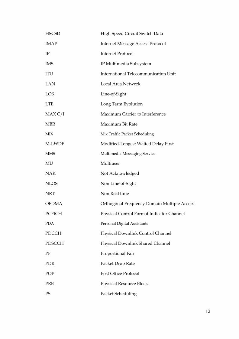
12
HSCSD High Speed Circuit Switch Data
IMAP Internet Message Access Protocol
IP Internet Protocol
IMS IP Multimedia Subsystem
ITU International Telecommunication Unit
LAN Local Area Network
LOS Line-of-Sight
LTE Long Term Evolution
MAX C/I Maximum Carrier to Interference
MBR Maximum Bit Rate
MIX Mix Traffic Packet Scheduling
M-LWDF Modified-Longest Waited Delay First
MMS Multimedia Messaging Service
MU Multiuser
NAK Not Acknowledged
NLOS Non Line-of-Sight
NRT Non Real time
OFDMA Orthogonal Frequency Domain Multiple Access
PCFICH Physical Control Format Indicator Channel
PDA Personal Digital Assistants
PDCCH Physical Downlink Control Channel
PDSCCH Physical Downlink Shared Channel
PF Proportional Fair
PDR Packet Drop Rate
POP Post Office Protocol
PRB Physical Resource Block
PS Packet Scheduling
13
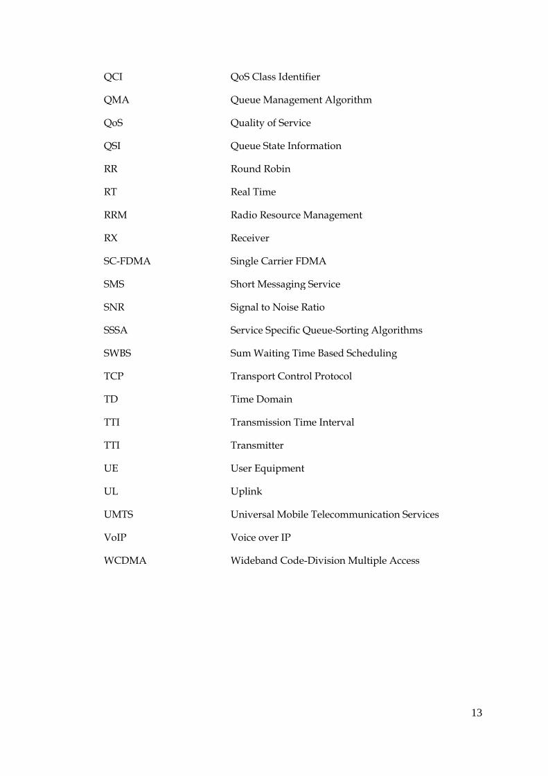
QCI QoS Class Identifier
QMA Queue Management Algorithm
QoS Quality of Service
QSI Queue State Information
RR Round Robin
RT Real Time
RRM Radio Resource Management
RX Receiver
SC-FDMA Single Carrier FDMA
SMS Short Messaging Service
SNR Signal to Noise Ratio
SSSA Service Specific Queue-Sorting Algorithms
SWBS Sum Waiting Time Based Scheduling
TCP Transport Control Protocol
TD Time Domain
TTI Transmission Time Interval
TTI Transmitter
UE User Equipment
UL Uplink
UMTS Universal Mobile Telecommunication Services
VoIP Voice over IP
WCDMA Wideband Code-Division Multiple Access
14
Chapter 1 Introduction
This chapter introduces the work presented in this thesis by briefly describing the
background knowledge and motivation of the work. The importance of the work is
described in the research scope section followed by the novel contributions of this thesis.
Background and Motivation 1.1
Long Term Evolution-Advanced (LTE-A) networks are envisioned to support wide range of
multimedia applications such as voice telephony, internet browsing, interactive gaming,
video messaging, email, etc. [3GP09]. These applications demand different Quality of
Service (QoS) requirements, such as average packet delay, average Packet Drop Rate (PDR),
and minimum throughput requirements [TCT10]. To fulfil diverse QoS requirements is
more challenging in wireless networks as compared to the wired networks. This is due to
the limited radio resources, the time-varying channel conditions and resource contention
among multiple users.
Packet scheduling deals with radio resource allocation and is directly related to the QoS
provision to users demanding different services. Three classic packet scheduling algorithms
are Round Robin (RR), Maximum Carrier to Interference (MAX C/I) and Proportional
Fairness (PF). These algorithms consider system-level performance such as fairness and
system spectral efficiency, and do not consider the QoS requirements of different services
from individual users. The current state of the art packet scheduling algorithms mainly take
QoS provision into consideration in order to provide better service experience for each
individual user. However, the performance of QoS aware packet scheduling algorithms at
both user-level and system-level has not been addressed properly.

15
The joint consideration of QoS provision at individual user-level and the overall system-
level performance is very crucial for an effective resource allocation. In this thesis a novel
QoS aware packet scheduling architecture is proposed which aims at improving the QoS
provision to different services while achieving a good trade-off between user-level and
system-level performance. The user-level performance is investigated by the QoS provision
to different services and for the system-level performance, system throughput, throughput
fairness among all users and average PDR fairness among all Real Time (RT) users are
considered.
Research Scope 1.2
This thesis describes research into the QoS aware scheduling in the Downlink (DL)of
Orthogonal Frequency Division Multiple Access (OFDMA) based LTE-A networks, by
addressing both user-level and system-level packet scheduling performance.
A cross-layer packet scheduling architecture is proposed and designed, which takes
information on service types, QoS requirements, queue states and channel states from
different protocol layers to take scheduling decisions.
At the user-level, a Traffic Differentiator stage is applied to segregate packet queues from all
active users into different service queues based on their service types. In each service queue,
users are prioritised according to their QoS requirement and wireless channel conditions by
implementing novel service-specific queue-sorting algorithms (SSSA).
At the system-level, fairness among users is one of the key attributes to be considered. In
multi-service networks such as LTE-A, it is important to allocate as fair share of available
radio resource as possible among all users, to avoid any service starvation. This thesis
proposes a novel Adaptive Time Domain Scheduling Algorithm (ATDSA) in the TD
16
Scheduler stage, which aims at allocating just enough radio resource to real-time and non-real
time services, and assigning the remaining available resource to the background service.
This is achieved by integrating Hebbian learning process and K-mean clustering algorithm
in ATDSA. Hebbian learning is applied to improve throughput fairness among all users and
K-mean clustering is applied to improve the average PDR fairness among users requiring
real-time service.
The FD Scheduler stage uses modified PF algorithm for resource allocation to exploit
Frequency Domain (FD) Multi User (MU) diversity.
Contributions 1.3
The work presented in this thesis is novel. The main contributions are:
A new cross-layer design QoS aware packet scheduling architecture for the DL transmission
of LTE-A networks, which incorporates different queue-sorting algorithm for each service
and integrates machine learning in the Time Domain (TD), to take adaptive scheduling
decisions. The feedbacks on Channel State Information (CSI) and information on parameters
such as QoS measurements and Queue State Information (QSI) are used at different stages of
the proposed architecture to make scheduling decisions adaptive to the service demands
and changing network scenarios.
A service-specific queue sorting algorithm is proposed for real-time voice service to
prioritise Real Time (RT) users based on their QSI including, Head of Line (HOL)
packet delay, delay budget and queue length, and CSI. This algorithm leads to
reduced, average packet delay, delay variation and average packet drop rate of real-
time service.
17
A service specific queue sorting algorithm is proposed for non-real time streaming
video service to prioritise Non Real Time (NRT) users based on the minimum
throughput requirements of this service, QSI including HOL packet delay and delay
budget and CSI. This algorithm meets the QoS requirements of streaming video
service better compared with conventional packet scheduling algorithms.
An adaptive time domain scheduling algorithm is proposed, which integrates
Hebbian learning process to adaptively allocate the available radio resource to all
services based on the average PDR information of real-time voice and non-real time
streaming video services. It allocates just enough radio resource to real-time and
non-real time services to meet their required QoS, and assigns the rest to the
background service. This algorithm with learning capability, leads to improved QoS
provision to real-time voice service and non-real time streaming video service. At the
same time, it improves the fairness at system-level by preventing background service
from starvation.
K-mean clustering algorithm is integrated into the time domain scheduling to
improve system-level performance in terms of average PDR fairness among RT
users. It leads to a significant reduction in average PDR variation of RT users,
especially in highly loaded network scenarios.
18
Author’s Publication 1.4
[Re-1] Rehana Kausar, Yue Chen, Kok. Keong. Chai, Laurie Cuthbert, John Schormans,
“ QoS aware Mixed Traffic Packet Scheduling in OFDMA-Based LTE-Advanced
Networks”, Fourth International Conference on Mobile Ubiquitous Computing
Systems, Services and Technologies 2010 (UBICOMM 2010), Florence, Italy,
October 25-30, 2010, [Best paper award].
[Re-2] Rehana Kausar, Yue Chen, Kok. Keong. Chai, “Service Specific Queue Sorting
and Scheduling Algorithm for OFDMA-Based LTE-Advanced Networks”, Sixth
International Conference on Broadband and Wireless Computing,
Communication and Applications (BWCCA), Barcelona, Spain, October 26-28,
2011.
[Re-3] Rehana Kausar, Yue Chen, Kok. Keong. Chai, “Adaptive Time Domain
Scheduling Algorithm for OFDMA Based LTE-Advanced Networks”, IEEE
Seventh International Conference on Wireless and Mobile Computing (WiMob),
Networking and Communications, 10 - 12 October 2011.
[Re-4] Rehana Kausar, Yue Chen, Kok. Keong. Chai, “ QoS Aware Packet Scheduling
with Adaptive Resource Allocation for OFDMA Based LTE-Advanced
Networks”, IET International Conference on Communication Technology and
Application (ICCTA), Beijing, China, 14-16 Oct 2011.
[Re-5] Rehana Kausar, Yue Chen, Kok. Keong. Chai, John Schormans, “ QoS Aware
Packet Scheduling Framework with Service Specific Queue Sorting and Adaptive
Time Domain Scheduling Algorithms for LTE-Advanced Downlink”,

19
International Journal on Advances in Networks and Services, ISSN 1942-2644,
Volume 4, numbers 3 & 4, pp. 244-256, 2011.
[Re-6] Rehana Kausar, Yue Chen, Kok. Keong. Chai, John Schormans, “ QoS Aware
Intelligent Scheduling Architecture for LTE-Advanced Networks”, The Research
to Industry Conference Henry Ford College, Loughborough (R2i)– 19th June
2012, an invited poster and oral presentation.
[Re-7] Rehana Kausar, Yue Chen, Kok. Keong. Chai, “An Intelligent Scheduling
Architecture for Mixed Traffic in LTE-Advanced”, 23rd IEEE International
Symposium on Personal, Indoor and Mobile Radio Communications (PIMRC)
2012. Sydney Australia, 9-12 Sep. 2012.
[Re-8] Rehana Kausar, Yue Chen, Kok. Keong. Chai, ““Broadband Wireless Access
Networks for 4G: Theory, Applications, and Experimentation”, IGI Global
(formerly Idea Group Inc.), contribution of one chapter accepted.
Thesis Organisation 1.5
The remaining thesis is structured as follows.
Chapter two presents background information on access technologies in cellular networks,
the principle of packet scheduling and the QoS architecture in LTE-A networks. This chapter
also describes classic packet scheduling algorithms and state-of-the-art on QoS aware packet
scheduling. In addition it gives an overview of incorporating machine learning processes in
scheduling with some learning algorithms.
Chapter three describes the research contributions of this thesis in detail. It describes the
cross-layer concept used in this research and the functionality of each stage of the proposed

20
packet scheduling architecture. The principle of all novel algorithms proposed at different
stages of the scheduling architecture such as algorithms in SSSA and ATDSA, are explained
in detail. At the end system-level performance evaluation indicators are given, which are
used to evaluate the performance of the proposed algorithms.
Chapter four describes the setup of the system-level simulation platform, used in this thesis
for performance evaluation. It includes the overall simulation structure, simulation
parameters and detailed functionality of the main simulation modules. It also describes the
wireless channel model used for this research. The important processes of validation and
verification, essential when using simulation-based research, are also described in this
chapter.
Chapter five presents simulation results from all proposed algorithms and their analysis, to
evaluate the proposed scheduling architecture. It presents simulation results of SSSA,
ATDSA, separately and jointly. The performance of the whole overall architecture is
analysed under different network scenarios. The simulation results are compared against the
state-of-the-art QoS aware Sum Waiting Time Based Scheduling (SWBS) and Mix Traffic
Packet Scheduling for UTRAN Long Term Evolution Downlink (abbreviated as MIX
hereafter) scheduling algorithms.
Chapter six concludes the work in this thesis. It presents the significant results and discusses
the potential future work.

21
Chapter 2 Research Study
This chapter describes in detail the fundamental technologies used in resource allocation in
different generations of mobile networks. The conventional and QoS-aware state-of-the-art
packet scheduling algorithms are investigated including machine learning based scheduling
in wireless networks. It also presents a study of service classes and service requirements
according to 3GPP specifications.
Access Technologies in Wireless Mobile Networks 2.1
Radio resource allocation schemes are closely related to the radio access technologies used in
mobile networks. In the last few decades, various radio access technologies have been
developed to enhance the resource allocation performance in mobile communication
networks. Figure 2-1 illustrates radio access technologies used in different generations of
mobile networks [GPKM08].
Figure 2-1 Evolution of access technologies in mobile cellular networks

22
The first generation (1G) radio communication systems like Advanced Mobile Phone System
(AMPS) or Nordic Mobile Telephone (NMT) were launched in 1970s, which use simple
analogue communication technology to provide voice call services [Yang05]. The second
generation (2G), Global System of Mobile Communications (GSM) commercially started in
1980s and it uses digital communication technique. GSM became the most commercially
successful 2G system as it was the first fully specified system with international
compatibility and transparency [KALNN05]. Until GSM, mobile networks had a circuit
switched core network. However in 1990s, a packet switched core network was added on
the top of the traditional circuit switched GSM network under the name General Packet
Radio Service (GPRS). It started to provide basic packet based services to the mobile users
such as Internet over the Wireless Application Protocol (WAP). However in the first version
of GPRS, QoS was supported only at the core network level as the GSM radio interface was
designed for circuit switched connections [KALNN05]. The development of the third
Generation (3G) systems was steered by the increasing demand of higher data rates. The
international standardisation body 3GPP (third Generation Partnership Project) started
specifications in 1998 of the Universal Mobile Telecommunication System (UMTS) with a
new air interface Wideband Code Division Multiple Access (WCDMA), for 3G networks
[Kumar09]. WCDMA allows a very flexible use of the available spectrum because of
advanced power control and Link Adaptation (LA) techniques and Universal Terrestrial
Radio Access Network (UTRAN). The flexibility of radio air interface makes QoS aware
Radio Resource Management (RRM) very crucial. High Speed Downlink Packet Access
(HSDPA) in an enhancement brought to UTRAN. HSDPA, among other technologies, brings
Packet Scheduler (PS) and LA closer to the air interface in the Base Station (BS), which
allows a faster adaptation to the channel conditions hence more flexibility and data rates
[HT07].The fourth Generation (4G) systems formalise the convergence between mobile

23
networks and wireless Local Area Network (LAN) systems into “broadband wireless
access” [Adachi02]. 3GPP has defined the standardisation for all Internet Protocol (IP)
mobile network systems Long Term Evolution (LTE), which applies the new RAN Evolved-
UTRAN (E-UTRAN). The E-UTRAN uses a simplified core network and RAN architecture
in order to reduce latency of packet based services. The new RAN is composed of only one
node, the evolved Node B (eNodeB/e-NB), which carries all RRM functionalities. LTE will
finally evolve into LTE-A networks.
The 2G GSM system applies both Time Division Multiple Access (TDMA) and Frequency
Division Multiple Access (FDMA) access technologies to allocate radio resource.
Figure 2-2 shows the principle of FDMA and TDMA technologies.
(a) FDMA (b) TDMA
Figure 2-2 FDMA and TDMA technology
In FDMA, signals for different users are transmitted on different frequency bands at the
same time. In TDMA, signals for different users are transmitted in the same frequency band
at different times [JWY05].
GSM network uses a combination of both FDMA and TDMA as air interface. The whole
spectrum is divided into fourteen bands with different frequencies. Each frequency band is

24
divided into eight time slots. Different users are allocated with different channels which
occupy different time slots on the same or different frequency bands.
In the 3rd Generation (3G) mobile cellular networks, Code Division Multiple Access
(CDMA) is adopted as the radio access technology [AG11]. Various standards are developed
for 3G systems which are used in different countries, such as WCDMA and Time Domain-
Synchronous Code Division Multiple Access (TD-SCDMA) for UMTS, and Multi-Carrier
CDMA (MC-CDMA) for CDMA2000 [JWY05] [OLDSMITH05]. The general principle of
CDMA is shown in Figure 2-3.
Figure 2-3 CDMA multiple access technology in 3G networks
In CDMA, signals for different users are transmitted in the same frequency band at the same
time but using different codes. As all signals are transmitted at same time and on the same
band so the capacity is mainly constrained by the interference between signals of different
users.
OFDMA in Long Term Evolution (LTE) Networks 2.2
LTE networks use OFDMA as the DL transmission technology and Single Carrier Frequency
Division Multiple Access (SC-FDMA) in the Uplink (UL) transmission technology [HT09].
These new technologies enable LTE networks to support a wide range of applications and to
meet the requirements set by 3GPP in terms of peak data rate, which is 100 Mbps for the DL

25
and 50 Mbps for UL and 1.5bps/Hz spectrum efficiency in a 20 MHz bandwidth. In some
countries, like the US and the UK, LTE networks have been commercialised. For further
development, 3GPP has started defining LTE-A in Release 10, which is expected to achieve
peak data rate up to 3 Gbps for the DL and 1.5 Gbps for the UL and 30 bps/Hz spectrum
efficiency in a 20 MHz bandwidth [KPKRHM08].
As this thesis only considers the DL transmission in LTE-A networks, therefore the DL radio
access technology OFDMA is describes in detail.
OFDMA is a multiple-access version of Orthogonal Frequency Division Multiplexing
(OFDM) scheme [Rappaport02]. The principle of OFDM is to use narrow, mutually
orthogonal sub-carriers to carry data, and OFDMA is achieved by assigning sub-channels to
carry data from different users. The OFDMA system assigns a subset of sub-carriers (termed
as OFDMA channel) to individual users. Each traffic channel is assigned exclusively to one
user at any time [3GPP09], as shown in Figure 2-3. In an OFDMA system, users are not
overlapped in the frequency domain at any given time; however, the frequency band
allocated to a particular user may change over the time. Figure 2-4 shows the principle of
radio resource allocation in OFDMA technology.
Figure 2-4 OFDMA technology

26
OFDMA is suitable for high data rate transmission in wideband wireless systems due to its
spectral efficiency and good immunity to multipath fading [AM08]. Moreover this
technology also provides a possible further enhancement to the system by enabling
opportunistic scheduling in the frequency domain. To frequency multiplex users in LTE,
sub-carriers are divided into sub-channels and each sub-channel or Physical Resource Block
(PRB) is composed of several neighbouring sub-carriers. By grouping the sub-carriers into
sub-channels or PRBs, the amount of control signalling and complexity of scheduling can be
reduced considerably [DPSB08]. Frequency domain packet scheduling which is used in LTE
is a powerful technique for improving the system capacity.
An important aspect of using OFDMA in LTE-A is that allocation is not done on individual
sub-carrier basis but is based on PRB. Each PRB consists of 12 sub-carriers and is equivalent
to a minimum bandwidth allocation of 180 kHz, where the respective allocation resolution
in the time domain is 1ms. The downlink transmission allocation thus means filling the
resource pool with 180 kHz blocks at 1 ms resolution as shown in Figure 2-5 [3GPP11].
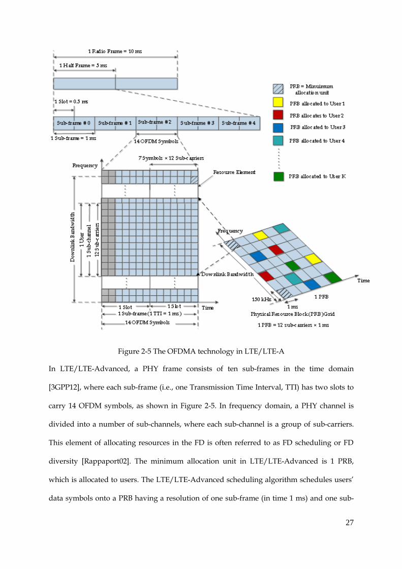
27
Figure 2-5 The OFDMA technology in LTE/LTE-A
In LTE/LTE-Advanced, a PHY frame consists of ten sub-frames in the time domain
[3GPP12], where each sub-frame (i.e., one Transmission Time Interval, TTI) has two slots to
carry 14 OFDM symbols, as shown in Figure 2-5. In frequency domain, a PHY channel is
divided into a number of sub-channels, where each sub-channel is a group of sub-carriers.
This element of allocating resources in the FD is often referred to as FD scheduling or FD
diversity [Rappaport02]. The minimum allocation unit in LTE/LTE-Advanced is 1 PRB,
which is allocated to users. The LTE/LTE-Advanced scheduling algorithm schedules users’
data symbols onto a PRB having a resolution of one sub-frame (in time 1 ms) and one sub-
28
channel (in frequency 180kHz). Different bandwidth spectrums use different number of
PRBs, i.e., a wider bandwidth spectrum includes more PRBs. For example, in the lowest
bandwidth of 1-4 MHz spectrum, a single channel consists of 6 PRBs and in the highest
bandwidth of 20 MHz, a single channel consists of 100 PRBs [3GPP11a].
Packet Scheduling 2.3
In a RAN, RRM is the set of components that helps achieving the required QoS while
efficiently using the available radio resources. Packet scheduling is one of the main RRM
functionalities and it is responsible for the selection of users and transmission of their
packets such that the available radio resource is efficiently utilised and the users’ QoS
requirements are satisfied.
Scheduling process deals with assigning the portions of available spectrum shared among
users, by following specific policies [TCT10]. The policy refers to the decision process used
to choose which users should be allocated radio resources in the given TTI and which users
should be delayed to the next TTI [Proacis01] [Jayakumari10] in order to provide the
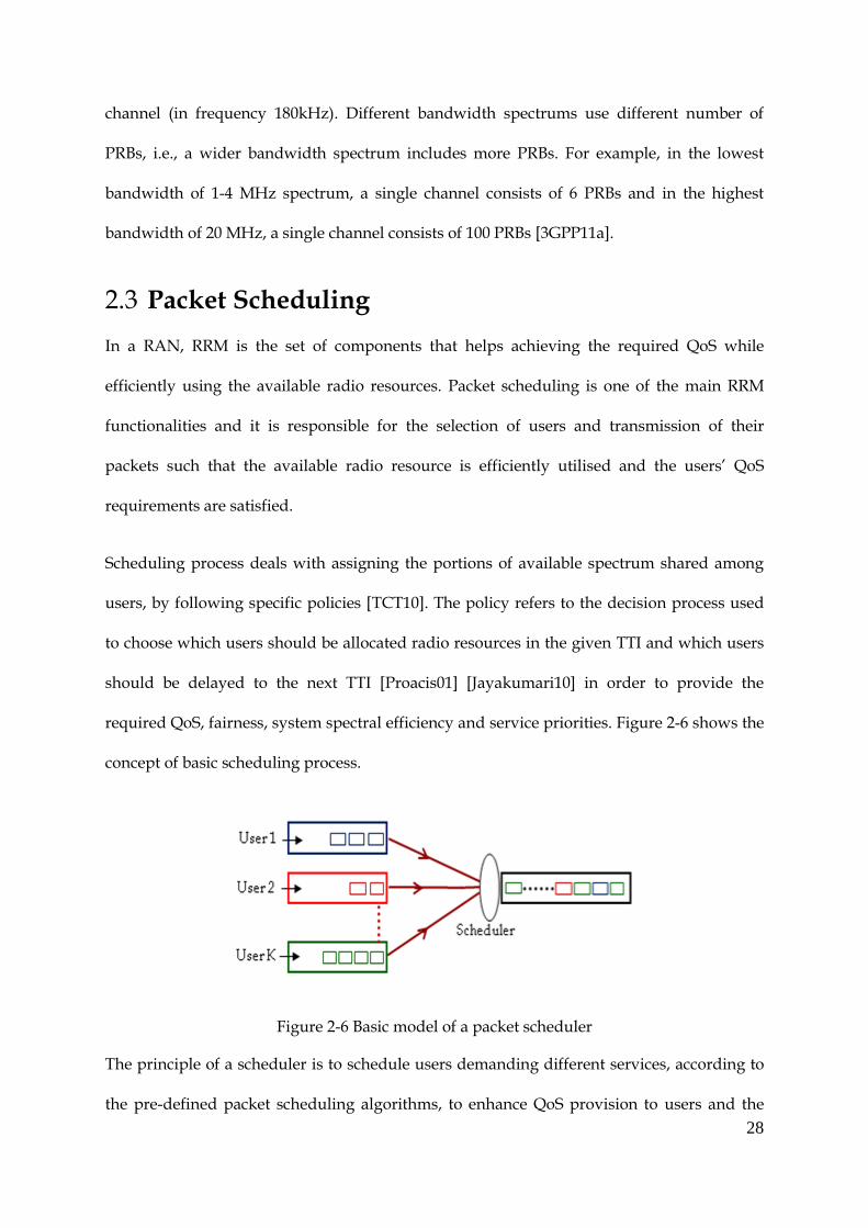
required QoS, fairness, system spectral efficiency and service priorities. Figure 2-6 shows the
concept of basic scheduling process.
Figure 2-6 Basic model of a packet scheduler
The principle of a scheduler is to schedule users demanding different services, according to
the pre-defined packet scheduling algorithms, to enhance QoS provision to users and the

29
system-level performance [ZP02]. These users demand different QoS requirements e.g. delay
and throughput. The scheduler takes into account of these requirements and schedules users
accordingly. Packets from the user queues are transmitted based on scheduler decisions.
Packet Scheduling is thus a method of network bandwidth management that can monitor
the importance of data packets and depending upon the priority of the packet, give it higher
or lower priority.
In [KSA08][HT09], a dynamic packet scheduler is defined as the main entity to take
scheduling decisions dynamically to ensure high spectral efficiency while providing
required QoS.
Different performance indicators have been used for evaluating performance of packet
schedulers in various research works. Main three are summarised as below.
QoS provision to different services: A QoS framework is a fundamental component
of the next generation broadband networks for satisfactory service delivery of
evolving Internet applications to the end users, and managing the network resources.
Today's popular mobile Internet applications, such as voice, gaming, streaming, and
social networking services, have diverse traffic characteristics and, consequently,
demand different QoS requirements. The data traffic associated with these services
must be delivered to the end users at specific data rates and/or within specific delay,
packet loss and delay variation bounds. These requirements can collectively be
termed as QoS. A rather flexible QoS framework is highly desirable to be future-
proof to deliver the incumbent as well as emerging mobile Internet applications.
System spectral efficiency: System spectral efficiency is typically measured in
bit/s/Hz (bit per second per Hz), bit/s/Hz/cell (bit per second per Hz per cell) or
bit/s/Hz/site (bit per second per Hz per site). It is a measure of the quantity of users

30
or services that can be simultaneously supported by limited radio frequency
bandwidth in a defined geographic area. It may for example be defined as the
maximum throughput, summed over all users in the system, divided by the channel
bandwidth.
Fairness among users: Fairness measures or metrics are used in network
engineering to determine whether users or applications are receiving a fair share of
system resources. In packet radio wireless networks, the fairly shared spectrum
efficiency (FSSE) can be used as a combined measure of fairness and system
spectrum efficiency. The system spectral efficiency (as described before) is the
aggregate throughput in the network divided by the utilized radio bandwidth in
hertz. The FSSE is the portion of the system spectral efficiency that is shared equally
among all active users. In case of scheduling starvation, the FSSE would be zero
during certain time intervals. In case of equally shared resources, the FSSE would be
equal to the system spectrum efficiency. Another fairness indicator is average PDR
fairness, which is achieved by reducing the variation in average PDR values of users.
In this thesis, the most commonly used performance metrics are adopted to validate the
effectiveness of the proposed scheduling architecture. They include average packet delay,
average PDR, throughput for different types of services, overall system throughput and
fairness.
Scheduling in LTE-A Networks 2.4
In LTE-A networks, all scheduling decisions whether it is UL or DL, are taken by eNB,
which is commonly known as Base Station (BS) in previous mobile generations. One of the
basic principles of the LTE/LTE-A radio access is shared-channel transmission which means
time-frequency resources are dynamically shared between users [DPSB08]. The scheduler is

31
a part of Medium Access Control (MAC) layer and controls the assignment of uplink and
downlink resources. The basic operation of the scheduler is so-called dynamic scheduling,
where eNB makes scheduling decisions and sends the scheduling information to the selected
set of terminals. The downlink scheduler is responsible for dynamically controlling the
terminals to transmit to; the set of resource blocks upon which the terminal’s DL Shared
Channel (DL-SCH) should be transmitted. The Physical Downlink Shared Channel (PDSCH)
carries the user data rate and the Physical Downlink Control Channel (PDCCH) informs the
device which resource blocks are allocated to it [DPSB08], dynamically with 1 ms
granularity. For the channel-dependent scheduling, the mobile terminals transmit channel
status reports reflecting the instantaneous channel quality in the time and frequency
domains. The channel status can be obtained by measuring the received transmission power
of the reference signals sent on the DL [DPSB08].
Sub-carriers
PDSCHPDCCH
Reference Signals
Figure 2-7 Reference signals
According to 3GPP standardisation, reference signals are embedded in the PRB as shown in
Figure 2-7. Based on the channel-status reports, the DL scheduler can assign resources for
downlink transmission to different mobile terminals. In principle, a scheduled terminal can

32
be assigned an arbitrary combination of 180k Hz wide resource block in each 1 ms TTI
[DPSB08].
During each TTI the eNB scheduler shall [3GPPLTE12d]:
Consider the physical radio environment conditions per User Equipment (UE): All
UEs report their perceived radio quality, as an input to the scheduler to decide which
modulation and coding scheme to use. The solution relies on rapid adaptation to
channel variations, employing Hybrid Automatic Repeat Request (HARQ) with soft-
combining and rate adaptation.
Prioritise the QoS service requirements amongst the UEs: LTE supports both delay
sensitive real-time services as well as data services that require high peak data rates.
It prioritises UEs according to their service requirements, to improve QoS provision.
Inform the UEs of allocated radio resources: The eNB schedules the UEs both on the
DL and on the UL. For each UE scheduled in a TTI, a Transport Block (TB) is
generated carrying user data, which is delivered on the transport channel. The
scheduled users are informed about their allocated resources before sending their
data. This information is called scheduling control information, which is sent on
control channel [3GPPLTE12d].
QoS Classes and QoS Requirements 2.5
From the end user’s point of view, the QoS of the service that the user has requested is
perceived by the user’s experience in relation to a particular application. For example, a web
browsing user perceives QoS mainly in terms of the time it takes until a webpage is fully
displayed after clicking on a hyperlink or entering a URL. From the technical point of view,
this duration results from a complex interaction of factors like throughput, packet delay, and

33
residual bit error ratio. Similarly, the quality of a Voice over IP (VoIP) call is perceived by
the end users in terms of delay and voice quality. Technically, the QoS of a VoIP call can be
expressed in packet delay and the residual bit error ratio.
In modern communication networks, there are more and more emerging services with
different QoS requirements which can be technically represented by different sets of QoS
parameters. This motivates the introduction of user experience classes that group together
services with similar QoS attributes. In [3GPP03] recommendation, this classification is as:
conversational class,
interactive class,
streaming class,
background class
In LTE-A, the conversational class includes basic conversational service, rich conversational
service and conversational low delay service as given in Table 2-1 [ 3GPP09c] [3GPP12a]. In
addition, it also supports interactive high and low delay service, streaming live and non-live
and background service.
Table 2-1 Service Classes

34
The basic conversational service class comprises basic services that are dominated by voice
communication characteristics. The rich conversational service class consists of services that
mainly provide synchronous communication enhanced by additional media such as video,
collaborative document viewing, etc. Conversational low delay class comprises real-time
services that have very strict delay requirements. In the interactive user experience class two
service classes are distinguished. Interactive services that permit relatively high delay which
usually follow a request-response pattern (e.g. web browsing, database query, etc.). In such
cases, response times in the order of a few seconds are permitted. Interactive services
requiring significantly lower delay is remote server access or remote collaboration. In the
streaming user experience class there are two service classes. The differentiating factor
between those two classes is the live or non-live nature of the content transmitted. In case of
live content, buffering possibilities are very limited, which makes the service very delay-
sensitive. In the case of non-live (i.e. pre-recorded) content, layout buffers at the receiver
side provide a high robustness against delay. The background class only contains delay-
insensitive services, so that there is no need for further differentiation [Jayakumari10].
Since classification of the services listed in Table 2-1 is based on user experience class and
service classes that are similar in terms of required QoS. The detailed services that are
combined into above mentioned service classes in Table 2-1 are represented in the Table 2-2
[3GPP07].

35
Table 2-2 Service Classification
User experience class
Service class Example services
Conversational Basic conversation Voice telephony (including VoIP), Emergency calling (call to public safety points), Push-to-talk (quick exchange of information).
Rich conversation Video conference, High-quality video telephony, Remote collaboration, e-Education (e.g. video call to teacher), Consultation (e.g. video interaction with doctor), Mobile commerce.
low delay Conversation
Interactive gaming, Consultation, Priority service.
Interactive Interactive high delay e-Education (e.g. data search), Consultation (e.g. data search), Internet browsing, Mobile commerce (buying/selling through wireless handheld devices), Location-based services (to enable users to find other people, vehicles, resources, services or machines).
Interactive low delay Emergency calling, e-mail (Internet Message Access Protocol, IMAP server access), Remote collaboration (e.g. desktop sharing), Push alerting (e.g. notification of hazardous situation), Messaging (instant messaging), Mobile broadcasting/multicasting (mobile interactive personalised TV), Interactive gaming.
Streaming Streaming live Emergency calling, Push alerting, e-Education (e.g. remote lecture), Consultation (e.g. remote monitoring), Machine-to-machine (e.g. observation), Mobile broadcasting/multicasting, Multimedia.
Streaming non-live Mobile broadcasting/multicasting, e-Education (e.g. education movies), Multimedia, Mobile commerce, Remote collaboration.
Background Background Messaging, Video messaging, Public alerting, e-mail (transfer Receiver /Transmitter, e.g. Post Office Protocol, POP), Machine-to-machine, File transfer/download, e-Education (file upload/download), Consultation (file upload/download), Internet browsing, Location-based service.

36
The QoS framework of LTE-A builds upon the one developed for LTE and allows the
support of wide range of services as described above. An end-to-end, class based QoS
architecture has been defined by LTE where a bearer is the level of granularity for QoS
control. It is much simpler than 3G networks and enables bearers to be mapped to a limited
number of discrete QoS classes. All network nodes can be pre-configured for these classes
limiting the QoS information which is needed to be dynamically signalled. The user-level
standardised QoS parameters are QoS Class Identifier (QCI), Allocation and Retention
Policy (ARP), Guaranteed Bit Rate (GBR), and Maximum Bit Rate (MBR). They are given in
Table 2-3 along with their brief description [3GPP12c].
Table 2-3 Bearer QoS Profile
QCI is used as a reference to access node-specific parameters that control bearer level packet
forwarding treatment (e.g. scheduling weights, admission thresholds, queue management
thresholds, link layer protocol configuration, etc.), and that have been pre-configured by the
operator owning the eNB. The goal of standardising a QCI with corresponding
characteristics is to ensure that applications/services mapped to that QCI receive the same
minimum level of QoS in multi-vendor network deployments [3GPP12c]. A standardised
QCI and corresponding characteristics is independent of the UE's current access (3GPP or
Non-3GPP). A one-to-one mapping of standardised QCI values to standardised
characteristics is for instance captured in [3GPP11b] for LTE. The configuration of those QoS

37
parameters allows LTE-A to support a wide range of services. Table 2-4 gives the QoS
parameters and priorities of different traffic types defined by 3GPP [3GPP12a].
Table 2-4 LTE QoS Class Identifiers and Service Priority
The QCI, as mentioned earlier, is a scalar that maps to a set of characteristics describing the
expected packet forwarding treatment. The GBR resource type provides the required GBR
while non-GBR does not provide any specific guarantee in terms of bit rate e.g. background
traffic. Priority 1 corresponds to the highest priority used to differentiate bearers in case of
resource shortage. Packet Delay Budget (PDB) is a soft upper bound with a confidence level
of 98% for a time that a packet may be delayed between the gateway and UE [GPKM08]. The
QCI 6, 8 and 9 apparently look similar however the QCI 6 can be used only if the network
supports Multimedia Priority Services (MPS), the QCI 8 is used for dedicated premium
bearer for any subscriber or group of subscribers and the QCI 9 is typically used for the
default bearer of a UE/PDN for non-privileged subscribers. More details on the QCI can be
found in [3GPP12a].
38
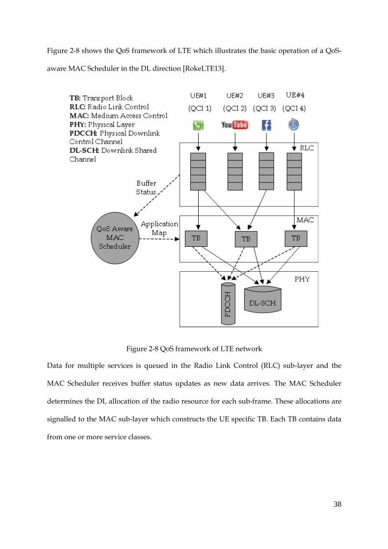
Figure 2-8 shows the QoS framework of LTE which illustrates the basic operation of a QoS-
aware MAC Scheduler in the DL direction [RokeLTE13].
Figure 2-8 QoS framework of LTE network
Data for multiple services is queued in the Radio Link Control (RLC) sub-layer and the
MAC Scheduler receives buffer status updates as new data arrives. The MAC Scheduler
determines the DL allocation of the radio resource for each sub-frame. These allocations are
signalled to the MAC sub-layer which constructs the UE specific TB. Each TB contains data
from one or more service classes.
39
Classic Packet Scheduling Algorithms 2.6
In this section, three classic packet scheduling algorithms RR, MAX C/I and PF are
described.
Round Robin (RR) Algorithm 2.6.1
The RR algorithm schedules users cyclically allocating a fair share of the available radio
resource to all users [TCT10]. In the wireless networks this algorithm is capable to achieve
starvation free scheduling. However the overall system throughput becomes low because
RR algorithm does not take into account of wireless channel conditions and cannot exploit
MU diversity. In general, MU diversity gain arises from the fact that in wireless systems
with a number of users, the utility value i.e. achievable data rate of a given resource block
varies from one user to another. This is because users have different channel conditions and
their achievable data rate varies [DPSB08]. These variations allow the overall system
performance to be maximised by allocating each resource block to the user that can best
exploit it [TCT10]. To illustrate MU diversity gain, an example of single cell OFDMA system
with two users is taken where users are scheduled by RR algorithm.
In this example, following assumptions are taken into account of.
1. Users’ channel responses are independent.
2. Users have perfect knowledge of channel state information.
3. There is perfect feedback from each user to the eNB.
4. The eNB gathers channel measurements from each user.
40
1H
2H
Static FDMA: Users are scheduled cyclically with static fraction of resources
Time (t)
Ch
ann
el G
ain
(H
)
User1 User2
User1
User2
1H 2H
System Throughput:
K
k
krR1
: Throughput of user kkr
User1 User2
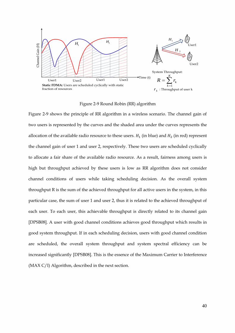
Figure 2-9 Round Robin (RR) algorithm
Figure 2-9 shows the principle of RR algorithm in a wireless scenario. The channel gain of
two users is represented by the curves and the shaded area under the curves represents the
allocation of the available radio resource to these users. (in blue) and (in red) represent
the channel gain of user 1 and user 2, respectively. These two users are scheduled cyclically
to allocate a fair share of the available radio resource. As a result, fairness among users is
high but throughput achieved by these users is low as RR algorithm does not consider
channel conditions of users while taking scheduling decision. As the overall system
throughput R is the sum of the achieved throughput for all active users in the system, in this
particular case, the sum of user 1 and user 2, thus it is related to the achieved throughput of
each user. To each user, this achievable throughput is directly related to its channel gain
[DPSB08]. A user with good channel conditions achieves good throughput which results in
good system throughput. If in each scheduling decision, users with good channel condition
are scheduled, the overall system throughput and system spectral efficiency can be
increased significantly [DPSB08]. This is the essence of the Maximum Carrier to Interference
(MAX C/I) Algorithm, described in the next section.

41
Maximum Carrier to Interference (MAX C/I) Algorithm 2.6.2
MAX C/I algorithm takes channel dependent scheduling decisions [PJNTTM03]. It basically
deals with the question of how to share available radio resources among users having
different channel conditions to achieve as efficient resource utilisation as possible [DPSB08].
It tries to exploit the channel variations through appropriate processing prior to
transmission of data. To increase system throughput (or system spectral efficiency), users
are scheduled when they have good channel conditions.
The MAX C/I algorithm schedules users with good channel conditions [HT09]
[PPMKRKM07]thus maximising the system throughput and thus system spectral efficiency.
In other words MAXC/I algorithm exploit MU diversity to maximise system spectral
efficiency. Figure 2-10 shows the scheme of MAX C/I algorithm.
3H
1H
2H
Dynamic OFDM: A user with the highest capacity is scheduled(exploitation of MU diversity)
Time
Ch
ann
el G
ain
(H
)
1H2H
fH3
User1
User2
User3
User 1 User2 User 1 User2
Figure 2-10 Maximum Carrier to Interference (MAX C/I) algorithm
A system of three active users is considered in Figure 2-10 in which three curves show the
channel gain of three users and the shaded area under the curves shows resource allocation
to these users. (in blue), (in red) and (in green) represent the wireless channel gain of
user 1, user 2 and user 3, respectively. A user is allocated radio resource only when it has
good channel conditions, as shown. User 1 and user 2 have good channel condition and are
scheduled but user 3 is never scheduled because it always has bad channel condition. As

42
MAX C/I algorithms schedules users only when they have good channel conditions, system
spectral efficiency is significantly increased as compared to the RR algorithm.
Generalising, a system consisting of number of users where and
number of available PRBs, where , the priority metric ( ) for MAX
C/I algorithm is given by Equation 2-1 [JNTMM08] [AKRSW01].
( ) ( ( )) (2-1)
In which ( ) is maximum instantaneous supportable data rate of user at time .
However in MAX C/I algorithm users with bad channel conditions, for example user 3 (in
green) in Figure 2-10, suffers starvation, which is not fair. The MAX C/I algorithm thus
achieves very low fairness as compared with RR algorithm.
A trade-off is needed between system spectral efficiency and user fairness to achieve an
efficient resource allocation. The PF algorithm is developed to make a good trade-off
between system spectral efficiency and user fairness [GBP08] [WXZXY03].
Proportional Fairness (PF) Algorithm 2.6.3
The PF algorithm takes both fairness among users and system spectral efficiency into
consideration and allocates the radio resource to users based on the ratio of their achievable
instantaneous throughput and their time averaged throughput [PBR05]. It allocates a fair
share of the radio resource to all users and maintains good system spectral efficiency at the
same time, by considering the trade-off between user fairness and system spectral efficiency.
43
Time
Dynamic OFDMA: A user with maximum ratio of achievable throughput to the mean throughput is scheduled
H
2H
3H
User 1 User2 User1 User3 User2
1H 2H
3H
Ch
ann
el G
ain
(H
)User1
User2
User3
User3
Figure 2-11 Proportional Fairness (PF) algorithm
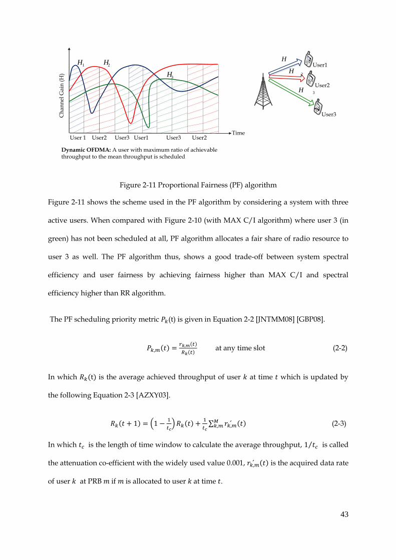
Figure 2-11 shows the scheme used in the PF algorithm by considering a system with three
active users. When compared with Figure 2-10 (with MAX C/I algorithm) where user 3 (in
green) has not been scheduled at all, PF algorithm allocates a fair share of radio resource to
user 3 as well. The PF algorithm thus, shows a good trade-off between system spectral
efficiency and user fairness by achieving fairness higher than MAX C/I and spectral
efficiency higher than RR algorithm.
The PF scheduling priority metric (t) is given in Equation 2-2 [JNTMM08] [GBP08].
( ) ( )
( ) at any time slot (2-2)
In which ( ) is the average achieved throughput of user at time which is updated by
the following Equation 2-3 [AZXY03].
( ) (
) ( )
∑ ́ ( ) (2-3)
In which is the length of time window to calculate the average throughput, ⁄ is called
the attenuation co-efficient with the widely used value 0.001, ́ ( ) is the acquired data rate
of user at PRB if is allocated to user at time .

44
Generalised Proportional Fairness Algorithm 2.7
The traditional PF scheduler allocates the user who maximises the ratio of achievable
instantaneous data-rate over average achieved data-rate [LL05]. The PF approach is
broadened to Generalised Proportional Fairness (GPF) algorithm [CJAN05]where new
weighting factors are introduced to the conventional PF algorithm. Referring to Equation 2-
2, GPF algorithm can be expressed as in Equation 2-4.
( ) [ ( )]
[ ( )] (2-4)
In Equation 2-4, by changing the values of parameters a and b, the trade-off between spectral
efficiency and fairness can be controlled. For a parameter setting conventional PF
scheduling is achieved and tuning between these parameters, the trade-off between fairness
and throughput can be tweaked. Increasing a will increase the influence of achievable
instantaneous data-rate which enhances the probability of a user in currently good condition
to be scheduled. This results in higher system spectral efficiency, but lower fairness.
Increasing b will increase the influence of the average data rate ( ) which increases the
probability of a user with a low average data rate to be scheduled thus increasing fairness
level of users.
QoS Aware Packet Scheduling Algorithms 2.8
The classic algorithms focus on fairness (RR algorithm), system spectral efficiency (MAX C/I
algorithm) or a trade-off between fairness and system spectral efficiency (PF algorithm).
However in the LTE-A networks, which aims to support diverse applications with variety of
QoS requirements, apart from system spectral efficiency and user fairness, the crucial point
is to meet users’ QoS requirements in a multi-service mixed traffic environment. For
example real-time services like audio phone and video conference require end-to-end

45
performance guarantees because a reliable and timely transmission is needed. On the other
hand non-real time services can tolerate delays to a certain limit but require long-term
minimum throughput guarantees.
The classic packet scheduling algorithms (section 2.2) cannot achieve the set targets by
International Telecommunication Union Recommendations (ITU-R) as they are only
designed to improve fairness, spectral efficiency or a trade-off between them.
The following section presents some of the state-of-the-art on QoS aware packet scheduling
algorithms followed by the motivation of the research work in this thesis.
Quality of Service (QoS) and Queue State Information 2.8.1
(QSI)
QoS is defined as the ability of a network to provide a service to an end user at a given
service-level where the service-level corresponds to end user experience such as packet
delay or data rate [SLC06]. QoS aware packet scheduling algorithms focus on meeting QoS
demands by using information on for example, channel and queue state.
In mixed traffic scenarios, QSI becomes important in addition to CSI [AZXY03]. It can make
scheduling decision even more efficient especially in the next generation of mobile
communication systems which support diverse range of applications. Typically this implies
to minimise the amount of resources needed per user and thus allows for as many users as
possible in the system, while still satisfying whatever quality of service requirements that
may exist [NH06]. Most of the QoS aware packet scheduling algorithms takes into account
of both QSI and CSI to make scheduling decisions to support QoS guarantees to different
service types.

46
Modified Largest Weighted Delay First (MLWDF) 2.8.2
Largest weighted delay first (LWDF) [SR00] is designed for the coexistence of real-time
services with different delay bounds but it cannot guarantee the throughput demands for
non-real time services [3CZWS10]. To provide QoS to different both real-time and non-real
time services, Modified Largest Weighted Delay First (MLWDF) algorithm was proposed in
[AKRS01]. It supports the guarantees of delay and minimum throughput requirements of
real-time and non-real time services, respectively in the third generation wireless networks.
In each time slot , it serves a queue that maximizes the following metric.
(2-5)
In which ( ) is the HOL packet delay for user queue , ( ) is the instantaneous
throughput with respect to flow , and are arbitrary positive constants, which embody the
QoS requirement, and provide QoS differentiation between the flows. In case of non-real
time service where the QoS requirement is minimum throughput instead of delay threshold,
this algorithm is modified by conjunction with a token bucket control. With each queue a
virtual token bucket is associated and tokens in the bucket arrive at the constant arrival
rate which is equal to the minimum throughput requirement of non-real time service. The
scheduling decision is taken by the same metric as for real-time service but ( ) being not
the delay of actual HOL packet of flow j but the delay of the longest waiting token in token
bucket . In this way MLWDF satisfies QoS of real-time and non-real time services in a TDM
system. However MLWDF does not consider system-level performance such as system
spectral efficiency and user fairness.
47
Subcarrier Allocation for OFDMA Systems 2.8.3
The MLWDF algorithm was extended to an OFDMA system in [PBA05]. Users are allocated
radio resources based on the product of their channel conditions and delay of the HOL
packet. Thus users with good channel conditions and longer waiting times are prioritised to
transmit their data. The algorithm, thus, prioritises a queue by the following metric.
[ ( )
( ) ( ) ( )] (2-6)
In which ( ) and ( ) are mean arrival and mean throughout respectively for flow j
averaged over a time period, is channel gain of user on subcarrier and ( ) is
delay of HOL packet of user . In this paper the delay of HOL is updated when all the
subcarriers are allocated which is not an accurate way of characterising the whole queue
status during a scheduling loop as it is exploited in MLWDF. Furthermore, the HOL delay
cannot be directly used for QoS guarantee of non-real time service as it does not embody
throughput requirements of it.
Sum Waiting Time Based Scheduling (SWBS) 2.8.4
In [SYLX09], a Sum Waiting Based Scheduling algorithm (SWBS) is presented which updates
the HOL delay after each subcarrier allocation instead of after allocating all subcarriers, to
make resource allocation accurate and fair as in [AKRS01]. Packet waiting time is used as a
metric for the satisfaction of real-time and non-real time services. However for non-real time
service, it is taken as virtual arrival time related to the minimum throughput of non-real
time service.
A PRB is allocated to a user based on the following metric.
[ ] ( ( ) [ ( )] ) (2-7)
48
In which ( ) is waiting time for user during time and [ ( )] is channel gain of
user on subchannel during time .
The waiting time for RT user is,
(2-8)
In which is the waiting time of packet of the user at time ,
is arrival time
of packet of user . The waiting time is summed up for all packets of a user and normalised
by delay budget (DB) of real-time service as given in Equation 2-9.
( )
∑
( ) (2-9)
In which ( ) is the queue length of user k. For non-real time service, waiting time of users
is calculated by considering virtual arrival time of users which is related with minimum
throughput requirements of non-real time service. This algorithm improves QoS to real-time
and non-real time services. However the system-level performance in terms of system
throughput and user fairness is not considered in the design of this algorithm.
Mixed Traffic Packet Scheduling in UTRAN (MIX) 2.8.5
In [JNTMM08], packet scheduling of mixed traffic in UTRAN LTE downlink is presented, in
which scheduling decisions are taken both in the time and frequency domains. The
scheduling unit is called a scheduling object, which corresponds to one UE with the
knowledge of traffic class, buffer sizes etc. The classifier divides different scheduling objects
into different traffic class dependent queues, TD scheduler chooses a certain number of
objects for scheduling candidates and FD scheduler does the actual PRB allocation. It uses
conventional algorithms (RR, MAX C/I and PF) to sort users in different queues. TD
scheduler uses either strict priority or fair scheduling algorithms in the TD scheduler to

49
select a pool of users from the head(s) of queue(s). In strict priority TD scheduling, queues
are emptied from top to bottom and in TD fair scheduling one user is picked from each
queue at a time. FD scheduler allocates PRBs to the candidate UEs chosen by the TD
scheduler. The scheduling scheme presented here is good however to improve QoS
provision instead of using conventional algorithms, service specific queue sorting
algorithms can be used. For example queuing delay aware sorting algorithms can be used
for VoIP, while the background could use e.g. proportional fairness algorithm.
Machine Learning in Scheduling 2.9
To enhance the scheduling performance in different domains, Artificial Intelligence (AI) can
be integrated in communication networks. The AI technologies offer many new and exciting
possibilities for the next generation of mobile communication networks [JN87]. Machine
learning is a branch of AI which deals with the study of systems that can learn from data.
For example, a machine learning system can be trained on email messages to learn to
distinguish between spam and non-spam messages. And after this learning, it can be used to
classify new emails into spam or non-spam folders.
In scheduling, data relevant to different parameters such as average PDR can be used to
train the system for the next scheduling decisions. As for example in this thesis, data on
average PDR of real-time service in previous TTIs is used as input in the Hebbian learning
process to train the system for taking adaptive scheduling decisions. Similarly average PDR
data of individual RT users is used in K-mean clustering algorithm to train the system to
prioritise users with higher average PDR values.
50
Hebbian Learning 2.9.1
One of the learning procedures for two-layer networks is the Hebbian Learning rule, which
is based on a rule initially proposed by Hebb in 1949. The Hebbian postulate of learning
discovered by Hebb [Hebb49] is one of the oldest learning rules. It states how much the
weight of the connection between two units should be increased or decreased in proportion
to the product of their activation [Hebb49] [WA93] [RM86]. The learning process extracts
information from environment and stores it in synaptic weights. Therefore at each step of
the learning process, an appropriate adjustment is applied to each synaptic weight. This
adjustment is represented for synaptic weight in the nth step by ( ) i.e.
( ) ( ) ( ) (2-10)
In which ( ) may have positive or negative values. A synapse that obeys Hebbian
learning rule is called a Hebbian synapse. A precise definition of Hebbian synapse is
proposed in [Haykin08]:
A synapse uses a time-dependent, highly local and strongly interactive mechanism to increase
synaptic efficiency as a function of the correlation between the presynaptic and postsynaptic
activities.
Hebbian learning process is adopted in this thesis because its computation time is smaller as
compared to other learning rules such as regressive learning and learning tree. It takes
decisions by extracting information from the environment and comparing current and
historical values of the extracted information. As the scheduling intervals are smaller and
quick decisions are needed in each interval, Hebbian learning process is thus appropriate to
adaptively allocate the available radio resource.

51
Previously, Hebbian learning rule was used in [KH10] for dynamic spectrum management
in Cognitive Radio (CR) to estimate the presence of primary users (PUs) in the environment;
PUs is the licensed users and allowed to operate in the spectrum band bought by the
wireless service provider. It helps in preventing collisions of CR units with PUs.
Clustering 2.9.2
Clustering is a grouping technology, which partition data into a number of clusters/groups
[XW05]. To deal with the variable QoS requirements of different users of a service type,
clustering is a suitable technique to integrate in scheduling algorithms to rearrange users’
priority according to their QoS requirements. More specifically, clustering is a technique to
group together a set of items having similar characteristics [SCDT00]. In scheduling domain,
where there is always a need to change priorities of different users according to their QoS
requirements, clustering is a good technique to construct groups of users with similar QoS
requirements. It helps in setting priorities of users by sorting these groups in an appropriate
way.
K-mean clustering algorithm is the most commonly used clustering algorithm, which is
adopted in many works [PKVP06] [PSPP07]]. It is incorporated in the proposed scheduling
architecture to improve the performance of real-time voice service.
K-mean clustering algorithm is used for partitioning (or clustering) N data points into Q
disjoint subsets containing data points so as to minimise the sum-of-squares criterion.
∑ ∑ | |
(2-11)
In which, is a vector representing the nth data point and is the geometric centroid of
the data points in .
52
The algorithm consists of a re-estimation procedure to group the given data into groups.
Initially, the data points are assigned at random to the Q sets. For step 1, the centroid is
computed for each set. In step 2, every point is assigned to the cluster whose centroid is
closest to that point. These two steps are alternated until a stopping criterion is met, i.e.,
when there is no further change in the assignment of the data points.
Clustering has already been used in many domains especially on web, such as aiming at
improving web applications [SCDT00] [PKVP06]. Clustering based scheduling gives
variable priorities to different users belonging to the same service type. For example in
[PSPP07], a clustering based scheduling algorithm is used to organise users of a network
into groups based on the number of their requests per channel. The transmission priority
then starts from the group with the highest requests. It improves network performance in
terms of higher network throughput while keeping mean packet delay at lower levels as
compared to the conventional scheduling algorithms [PSPP07].
Problem Description 2.10
Packet scheduling algorithms described above and in other existing literature are designed
to improve scheduling performance in different domains separately. For example they either
consider system-level scheduling performance i.e. system spectral efficiency and user
fairness or the user-level scheduling performance i.e. QoS of real-time and non-real time
services. However, at the time of this thesis being written, the joint consideration of user-
level and system-level performance of QoS aware packet scheduling has not been researched
in depth. As for example [JNTMM08] [LL05] focuses on performance enhancement on
fairness level and system spectral efficiency but lacks QoS support to different services. And
the scheduling schemes in [SR00] [3CZWS10] [AKRS01] [PBA05] [SYLX09] mainly address

53
the support of QoS to real-time and non-real time services but do not investigate the system–
level performance in terms of spectral efficiency and fairness.
As in a MU environment, the radio resources are shared among multiple users. A wireless
network must be able to serve a diverse set of users in a highly dynamic, resource
constrained and data intensive environments [PR80]. In a large scale wireless network,
user’s channel conditions, queue status and traffic type requirements are highly diverse.
Therefore each radio resource in the time-frequency dimension is likely to have high utility
value to certain users. Consequently, the total channel capacity or spectral efficiency of the
network can be significantly increased through effective resource allocation in MAC layer.
This motivates the design of highly adaptive MAC layer protocols and algorithms that can
cope with the channel and traffic dynamics [KSA08], to achieve better resource allocation.
The work in this thesis addresses the scheduling problem in a multi-service mixed traffic
environment for the DL transmission of LTE-A networks where the competition to get radio
resources is very high and there are strict QoS requirements. In such environment, the
crucial point is to clearly define the QoS requirements of different traffic types, their
demands for radio resources, their channel conditions and queue status to support their
demands. Combined consideration of this information can lead to a more efficient packet
scheduling algorithm in terms of both the user-level performance and the system-level
performance. An intelligent packet scheduling architecture can achieve this goal by making
scheduling decisions adaptive to the network scenarios and also adaptive to the achieved
performance of different services measured by QoS parameters.
54
Summary 2.11
In this chapter background knowledge of radio access technologies, packet scheduling,
packet scheduling in OFDMA-based LTE-A networks, classic packet scheduling algorithms,
QoS aware packet scheduling and machine learning based scheduling is presented. The
state-of-the-art QoS aware algorithms are also discussed followed by the problem
formulation which leads to the motivation of the research work in this thesis. The detail of
the proposed research work is given in the next chapter, which includes the description on
all novel algorithms presented in this thesis.

55
Chapter 3 Cross-Layer Design for QoS Aware
Scheduling Architecture
This chapter presents the proposed cross-layer packet scheduling architecture and all novel
algorithms used in it are described in detail. The concept of cross-layer design and the
system model used in this thesis are explained comprehensively. At the end, it gives system-
level performance evaluation parameters with their short description.
Principle of Design of Scheduling Architecture 3.1
A schematic diagram of the proposed Cross-Layer QoS Aware Packet Scheduling
Architecture (CLPSA) is shown in Figure 3-1. It divides the scheduling process of the Time
Domain (TD) and Frequency Domain (FD) into three stages; the Traffic Differentiator, the TD
Scheduler and the FD Scheduler. These stages serve different functionalities by utilising
information from different layers and work together to achieve better QoS for different
services (user-level performance), and to achieve a good trade-off between the user-level
and the system-level performance.
Figure 3-1 Cross-layer QoS aware packet scheduling architecture
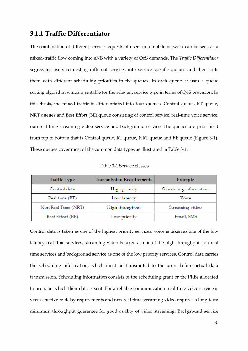
56
Traffic Differentiator 3.1.1
The combination of different service requests of users in a mobile network can be seen as a
mixed-traffic flow coming into eNB with a variety of QoS demands. The Traffic Differentiator
segregates users requesting different services into service-specific queues and then sorts
them with different scheduling priorities in the queues. In each queue, it uses a queue
sorting algorithm which is suitable for the relevant service type in terms of QoS provision. In
this thesis, the mixed traffic is differentiated into four queues: Control queue, RT queue,
NRT queues and Best Effort (BE) queue consisting of control service, real-time voice service,
non-real time streaming video service and background service. The queues are prioritised
from top to bottom that is Control queue, RT queue, NRT queue and BE queue (Figure 3-1).
These queues cover most of the common data types as illustrated in Table 3-1.
Table 3-1 Service classes
Control data is taken as one of the highest priority services, voice is taken as one of the low
latency real-time services, streaming video is taken as one of the high throughput non-real
time services and background service as one of the low priority services. Control data carries
the scheduling information, which must be transmitted to the users before actual data
transmission. Scheduling information consists of the scheduling grant or the PRBs allocated
to users on which their data is sent. For a reliable communication, real-time voice service is
very sensitive to delay requirements and non-real time streaming video requires a long-term
minimum throughput guarantee for good quality of video streaming. Background service

57
however does not have any QoS requirements, thus, comes in the category of low priority
services. Control information of all scheduled users is transmitted in First Come First Serve
(FCFS) manner. Two novel Service Specific queue Sorting Algorithms (SSSA) are proposed
for real-time voice and non-real time streaming service. The users requesting background
service are prioritised by using PF algorithm to maintain a good trade-off between fairness
and system throughput.
TD Scheduler 3.1.2
The TD Scheduler makes decision on which users should be scheduled in the current TTI by
considering both the available radio resource and the priorities of different users. An
Adaptive Time Domain Scheduling Algorithm is proposed in the TD Scheduler stage, which
incorporates Hebbian learning process and K-mean clustering algorithm, to achieve
adaptive resource allocation. Hebbian learning is applied to decide how many RT, NRT and
BE users should be scheduled in the current TTI. It makes a good balance of resource
allocation among different service types in order to achieve a good system-level
performance. K-mean clustering algorithm is used to further arrange the priorities of
selected RT users based on their individual PDR in order to achieve better PDR fairness and
reduced average delay of RT users.
FD Scheduler 3.1.3
The FD Scheduler makes the decision on the actual mapping of PRBs to the selected users
from the TD scheduler. MU diversity is exploited in the frequency domain to allocate the best
possible PRB to each selected user. Followed by the actual resource allocation decision, the
QoS measurement unit calculates the average throughput of NRT users, average delay and
average PDR of RT users and sends this information to the TD scheduler stage as part of the
inputs for decision making in the next TTI. The CQI report from all users is assumed to be

58
accurate and available to eNB in each TTI, as considered in most of the literature on channel
aware scheduling.
Cross-Layer Concept 3.1.4
The cross-layer concept in the proposed architecture is used by taking information from
different layers for making scheduling decisions, as shown in Figure 3-2. For each user, the
Traffic Differentiator takes the traffic type information from the application layer, QoS
requirements (e.g. delay budget or minimum throughput required) information from the
network layer, the queue status information from the Radio Link Control (RLC) layer and
the channel status information from the physical layer. The TD scheduler takes QoS
measurements on average PDR from the MAC layer as part of the inputs for the Hebbian
learning and the K-mean clustering algorithm. The FD scheduler makes the PRB mapping
based on user priorities and per PRB CQI reports.
Applications
DataTraffic
Classification
RT NRT BE C
Scheduler
Application layer(Traffic type/content)
Network layer (QoS information)
MAC sub-layerQoS aware TD & FD
scheduling
Physical layerPer user & per PRB CQI
Input
Traffic Differentiator
TD/FD Scheduler
CQI
RLC sub-layer (Buffer status)
Figure 3-2 Cross-layer design for QoS aware scheduling architecture
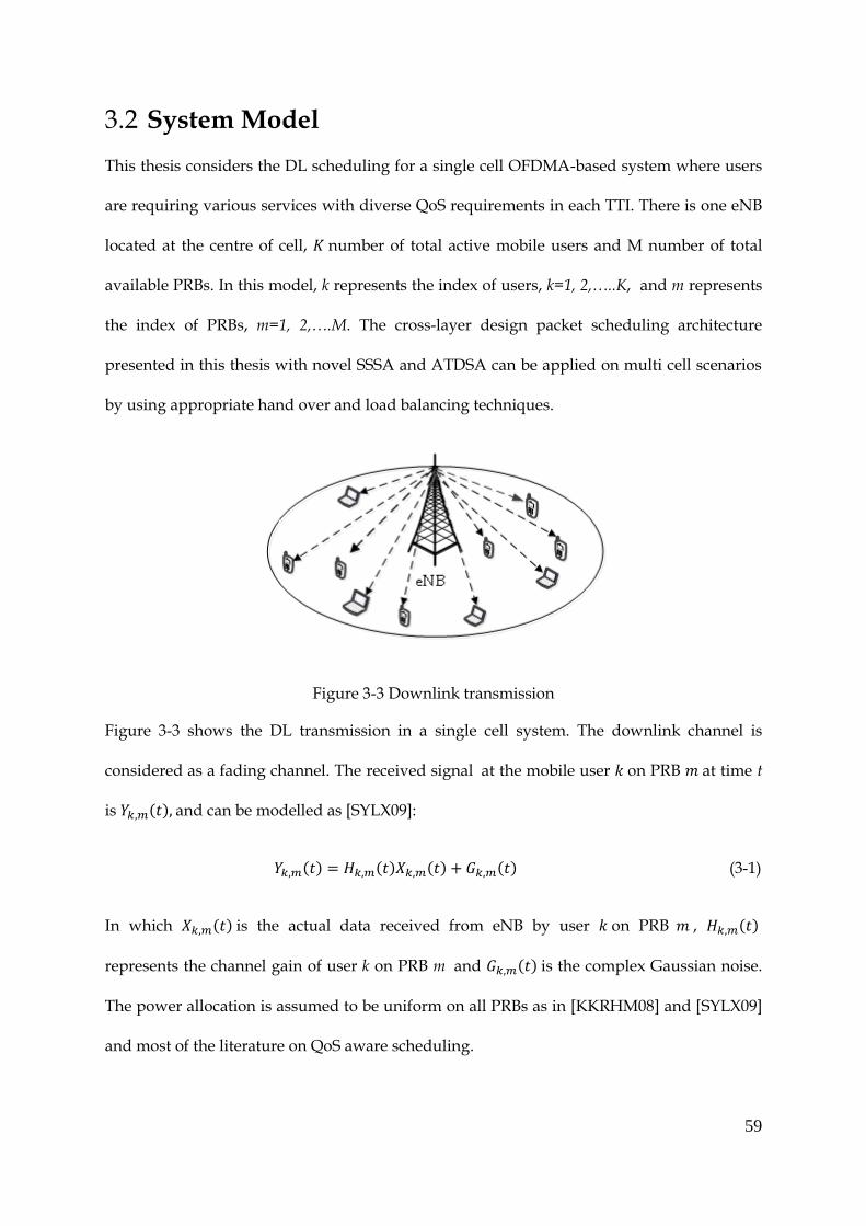
59
System Model 3.2
This thesis considers the DL scheduling for a single cell OFDMA-based system where users
are requiring various services with diverse QoS requirements in each TTI. There is one eNB
located at the centre of cell, number of total active mobile users and M number of total
available PRBs. In this model, k represents the index of users, k=1, 2,…..K, and m represents
the index of PRBs, m=1, 2,….M. The cross-layer design packet scheduling architecture
presented in this thesis with novel SSSA and ATDSA can be applied on multi cell scenarios
by using appropriate hand over and load balancing techniques.
Figure 3-3 Downlink transmission
Figure 3-3 shows the DL transmission in a single cell system. The downlink channel is
considered as a fading channel. The received signal at the mobile user on PRB at time t
is ( ) and can be modelled as [SYLX09]:
( ) ( ) ( ) ( ) (3-1)
In which ( ) is the actual data received from eNB by user on PRB , ( )
represents the channel gain of user k on PRB m and ( ) is the complex Gaussian noise.
The power allocation is assumed to be uniform on all PRBs as in [KKRHM08] and [SYLX09]
and most of the literature on QoS aware scheduling.

60
The channel capacity of user on PRB can be expressed as [JL03]:
( ) ( | ( )|
( )
) (3-2)
In which, B is the total available bandwidth, is the data rate that can be achieved by
user if allocated with PRB , is the power allocated to user at PRB , is the
variance of Additive White Gaussian Noise (AWGN) and г is called Signal to Noise Ratio
(SNR) gap and is a function of target Bit Error Rate (BER). For AWGN channel, it can be
expressed as г, ( )⁄ [GS97].
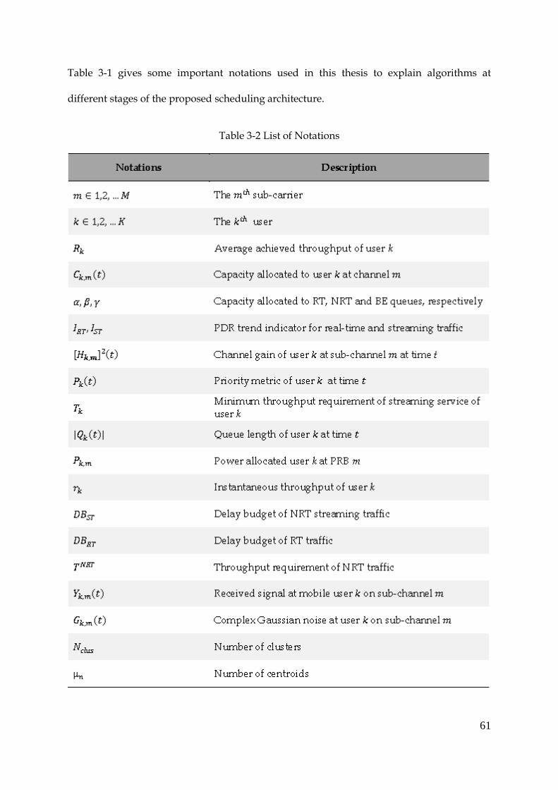
61
Table 3-1 gives some important notations used in this thesis to explain algorithms at
different stages of the proposed scheduling architecture.
Table 3-2 List of Notations

62
Queue Sorting Algorithms in Traffic Differentiator 3.3
Two novel service-specific queue-sorting algorithms (SSSA) are proposed to prioritise users
in RT and NRT queues, respectively in the Traffic Differentiator stage. This section describes
the principle of these algorithms and the performance metrics used to evaluate the
performance of these two algorithms.
Figure 3-4 shows the detailed functionality of Traffic Differentiator which mix traffic is
differentiated into RT voice users, NRT streaming users, background or BE users and their
control information is put in a separate queue. These four categories resemble four queues in
Figure 3-1. Users carry their data packets in their individual queues, as shown in Figure 3-4.
User 1 User 2 User 3 User K
Mixed Traffic
Traffic Differentiator
RT NRT BE
RT voice users NRT streaming users Best Effort users
Co
ntr
ol
Dat
a Q
ueu
e
QSI
tQHOL k,
CSI
CQISNR ,Receive from Receiver
Class K
Obtained from Queue
Phase 1: SSSAService Specific Sorting Algorithm
Figure 3-4 Traffic differentiator Stage
In each service queue, users require the same type of traffic e.g. Control queue contains only
control information of all users, users in RT queue require voice service, users in NRT

63
queue require streaming service and in BE queue users require background service. Users in
these queues are sorted from the highest scheduling priority to lowest scheduling priority
by applying SSSA, which uses QSI, QoS and CQI information.
The detailed description of queue sorting algorithms is given below.
FCFS Algorithm for Control Traffic Queue 3.3.1
Control information is transmitted on Broadcast Control Channel (BCCH) which is a
downlink channel for broadcasting system control information [HAJMSIM06]. The control
information consists of three types of information.
scheduling information for DL data transmission,
scheduling grant for UL transmission and
ACK/NAK in response to UL transmission.
The control information needs to have the highest scheduling priority as it contains essential
information to facilitate the actual resource allocation. Hence the control information is put
into a dedicated queue and scheduled before all other service queues. As the control
information of all users is equally important therefore it is proposed to transmit it in a FCFS
manner. Physical Control Format Indicator Channel (PCFICH) dynamically indicates how
many OFDMA symbols are reserved for transmitting control information. This can vary
from 1 and 3 for each 1 ms sub-frame as shown in Figure 3-5 [HT09].

64
Figure 3-5 PDCCH resource allocation from PCFICH
Figure 3-5 shows the resource adjustment of PDCCH indicated by PCFICH. This thesis
considers scheduling for DL data transmission, the control queue contains only scheduling
information for the DL data transmission. And it is assumed that 1 OFDMA symbol per sub-
frame is reserved for control information in each TTI for each user, which is enough for DL
scheduling information. Thus, 1 OFDMA symbol/user is always reserved to transmit
control data for the DL scheduling of each scheduled user in each TTI. For the resource
allocation to remaining queues (RT, NRT and BE), the available PRBs are considered as the
total number of PRBs subtracted by number of PRBs reserved for the control queue.
In this way, the control queue is always prioritised over other queues and is always
allocated enough resources to transmit control information of the scheduled users.

65
Novel Queue Sorting Algorithm for RT Queue 3.3.2
The novel queue-sorting algorithm for RT queue considers the QoS requirements of real-
time service and sorts users in this queue accordingly. In mobile networks, packet delay of
users is considered an important parameter to evaluate the performance of real-time service.
The packet delay experienced by RT users must be lesser than the delay upper bound,
where is the delay of HOL packet of user and is the upper bound or
the delay budget for real-time service. HOL packet is the one ready to be scheduled i.e. at
the front of user packet queue. If a user’s HOL packet has delay more than delay upper
bound , it is dropped from the queue otherwise it is scheduled. In addition to packet delay,
this thesis considers two more performance indicators for real-time service; average PDR of
real-time service and average PDR variation of RT users. These two parameters are
discussed in detail in sections (3.4.1) and (3.4.2) respectively. The users in RT queue are
sorted to give higher priority to the users with higher packet delays, longer waited queues
and good channel conditions.
In the queue-sorting algorithm used for RT queue the priority metric is formed by the
product of normalised HOL packet delay and the complex channel gain of the users, which
is added to the square of the queue length of users as given in Equation 3-3. The normalised
HOL delay is a ratio of user’s HOL packet’s waiting time and the delay budget for real-time
service. The priority of user at time , ( ) is,
( ) ( ( ) [
( )] ) [ ( )]
(3-3)
In which [ ( )]
is the channel gain of RT user at time t, ( ) is the queue length of
user at time and ( ) is normalised HOL delay of user k at time t, which is given by
Equation 3-4.

66
(3-4)
In which is the HOL packet delay of RT user k, which is very important to be
considered because real-time service is highly delay-dependent. This parameter is updated
in each TTI and it keeps packet delay under the delay budget. The rationale behind
considering queue length of users is to further reduce the delay of RT users by allocating
more resources to users with longer queues. Moreover the square of queue length is taken to
increase the weight of queue length in the priority metric. This is because queue length is
very important parameter to be considered in order to control the PDR of RT users. Also the
priority metric considers the data rate of users by prioritising users with good channel
conditions. It comes up with improvement in overall system spectral efficiency as well.
In the queue sorting process, users are sorted in descending order of this priority metric and
users with higher values have higher priority.
The proposed delay-dependent queue sorting algorithm in Equation 3-3 leads to reduced
packet delay of real-time service resulting in lower PDR.
This algorithm is able to control delay of RT users by appropriately setting priority level to
different users.
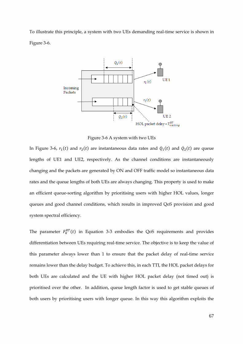
67
To illustrate this principle, a system with two UEs demanding real-time service is shown in
Figure 3-6.
Figure 3-6 A system with two UEs
In Figure 3-6, ( ) and ( ) are instantaneous data rates and ( ) and ( ) are queue
lengths of UE1 and UE2, respectively. As the channel conditions are instantaneously
changing and the packets are generated by ON and OFF traffic model so instantaneous data
rates and the queue lengths of both UEs are always changing. This property is used to make
an efficient queue-sorting algorithm by prioritising users with higher HOL values, longer
queues and good channel conditions, which results in improved QoS provision and good
system spectral efficiency.
The parameter ( ) in Equation 3-3 embodies the QoS requirements and provides
differentiation between UEs requiring real-time service. The objective is to keep the value of
this parameter always lower than 1 to ensure that the packet delay of real-time service
remains lower than the delay budget. To achieve this, in each TTI, the HOL packet delays for
both UEs are calculated and the UE with higher HOL packet delay (not timed out) is
prioritised over the other. In addition, queue length factor is used to get stable queues of
both users by prioritising users with longer queue. In this way this algorithm exploits the
68
variable channel and queue states and updates the priority of users accordingly to meet QoS
demands of real-time service.
Novel Queue Sorting Algorithm for NRT Queue 3.3.3
NRT queue in the scheduling architecture consists of users requiring non-real time
streaming video service. The novel queue-sorting algorithm for NRT queue sorts users in the
queue according to the throughput requirement of streaming video service. The basic QoS
requirement for streaming video service is the provision of long-term minimum throughput
guarantee. Therefore QoS for streaming traffic is evaluated by the average achieved
throughput of users of NRT queue. It must be equal to or greater than the minimum
throughput requirements of streaming service, , in which is instantaneous
throughput and is minimum throughput requirement of streaming service. The minimum
throughput requirement is taken as 240kb/s in this thesis as in [SYLXSYLX09]. To meet the
requirement, this algorithm is designed to maximise the minimal throughput among all
NRT users, which is given in Equation 3-5.
{ ∞∑ ( ) } (3-5)
The minimal throughput among all NRT users is given by Equation 3-6 as used in
[SYLXSYLX09].
( ) (3-6)
To achieve this, the users in this queue are sorted to give priority to the users with low
average achieved throughput.
The priority metric for streaming service is the product of the normalised HOL packet delay
of each user, the ratio of its required throughput to the average throughput over a given

69
time interval and the channel gain. The priority metric considers the product of these
parameters to give equal weight to all parameters included in it. This is because these
parameters equally contribute to the effective resource allocation to users belonging to the
NRT queue.
The priority metric of user at time ( ) is:
( ) ( ) ( ) [
( )] (3-7)
In which, ( ) is the normalised HOL packet delay of NRT user k, ( )is the ratio of
required throughput of streaming service to the average achieved throughput of NRT users
and [ ( )]
is channel gain of NRT user k, at time t. The channel conditions of users are
considered while prioritising users in the queue to improve the data rate of users thus
improving overall system spectral efficiency.
The value of is given in Equation 3-8 and the value of is given in Equation 3-9.
(3-8)
In which NRTDB is delay budget for streaming video service. To reduce the delay of
streaming video packets, it is important to consider HOL packet delay of users belonging to
this queue.
The parameter embodies the throughput requirements of streaming video service. The
value of for NRT user at time t can be calculated by Equation 3-9.
( ) ( )
( ) ( ( ) ) (3-9)
In which ( ) is the minimum required throughput of user at time , and ( ) is its
average achieved throughput which is calculated by (2-3). The rationale behind using this

70
parameter is to keep each user’s average achieved throughput equal or greater than the
minimum throughput requirements of streaming service. As the main evaluation parameter
for streaming service is minimum required throughput, it is very important to take into
account of the minimum throughput requirements of it while prioritising users in this
queue. To understand the logic of how this parameter leads to meet minimum throughput
requirements, consider the following two cases.
Case 1:
In each TTI the value of is calculated to evaluate the performance of streaming video
service. Case 1 shows one scenario in which the average achieved throughput of user is
lower than its minimum throughput requirement.
( ) ( )
( ) (3-10)
Or, ( ) ( )
If the value of ( ) is higher than one, it shows that the average achieved throughput of
user k at time t is lower than the minimum throughput requirement of streaming video
service. If this is the case the priority of user is increased in the next TTI to meet the
throughput requirements. This is achieved by considering the parameter in queue-sorting
algorithm for NRT queue. As given in Equation 3-7, the higher the value of , the higher is
priority of user k.

71
Case 2:
Case 2 shows that the average achieved throughput of user is higher than or equal to its
minimum required throughput.
(3-11)
Or,
If the value of is equal to or lower than one, it shows that the average achieved
throughput of user k is equal to or higher than the minimum throughput requirement. In
this case the priority of user k is either decreased ( ) or is kept same ( ).
In each TTI is updated and users are prioritised accordingly, to meet throughput
requirement of NRT users.
PF Algorithm for BE Queue 3.3.4
The BE queue in the proposed scheduling architecture represents the background service
and does not have any QoS requirements. The priority is, thus, given to BE users based only
on channel conditions. However to maintain fairness among users, the PF algorithm is used
as the queue sorting algorithm for BE queue.
The priority of user in BE queue at time , ( ) is:
( ) ( )
( ) (3-12)
In which is instantaneous throughput and is the average throughput of user at time .
72
Machine Learning Algorithms in TD Scheduler 3.4
Packet scheduling is mainly focused on PRB allocation based on users’ CSI, QCI information
and QoS requirements. However because of ever increasing number of mobile users and
limited number of available PRBs, it is difficult to guarantee all on-going users’ QoS during
the same TTI. Here arises the need of a TD scheduling algorithm to make decisions
adaptively whether to admit or delay scheduling request of users, before actually allocating
the radio resource to users in FD scheduling in each TTI. A novel Adaptive Time Domain
Scheduling Algorithm (ATDSA) is proposed in this thesis which selects a pool of users
adaptively from the service queues based on their priorities and the available radio
resources users. It uses average PDR value of real-time voice & non-real time streaming
video services to select a pool of users from the user queues.
The average PDR is calculated by Equation 3-13.
∑
(3-13)
In which
is the total number of packets dropped for user , is total number of
packets arrived for user and K is total number of active users.
This novel ATDSA works in the second stage of CLPSA, TD Scheduler that incorporates
Hebbian learning process and K-mean clustering algorithm. Hebbian learning process is
applied for adaptively allocating just enough radio resources to different services based on
the average PDR of real-time and streaming services. K-mean clustering algorithm utilises
average PDR information of individual RT users to further arrange the priority of RT users
selected in Traffic Differentiator stage.

73
Figure 3-7 shows the second stage of CLPSA with two main process; Hebbian learning and
K-mean clustering. These processes are described in detail in sections (3.4.1) and (3.4.2).
TD Scheduler
Hebbian Learning ProcessTakes adaptive decisions on
resource allocation
Ave PDRinformation
Traffic Differentiator
FD Scheduler
K-mean Clustering ProcessRe-prioritises selected
RT users
Stage 2: ATDSAAdaptive Time Domain Scheduling Algorithm
Figure 3-7 TD scheduler stage
Hebbian learning Process in ATDSA 3.4.1
Hebbian learning process takes decisions on radio resource allocation to real-time voice,
non-real time streaming video and background services by adjusting the weight of these
services during each TTI based on the average PDR values of the first two services. The aim
is to allocate just enough resources to real-time voice and non-real time streaming video
service, and assign the rest of radio resource to the background service.
In this process x, y and z are the weights of radio resource which should be allocated to real-
time voice, non-real time streaming and background services, respectively such that,
(3-14)

74
The initial values of x, y and z are calculated based on the ratio of the number of active users
in each of service type to the total number of active users in the system. It is given in
Equation 3-15.
{
(3-15)
In which, X, Y and Z represent the number of active users in real-time voice, non-real time
streaming video and background service, respectively. The number of PRBs allocated to
real-time voice, non-real time streaming and background services are represented by α, β
and γ, respectively. The initial values of α, β and γ, are calculated by multiplying the
rounded off values of x, y and z to the total number of available PRBs.
{
( ) ( ) ( )
(3-16)
In which M is the total number of PRBs subtracted by the number of PRBs reserved for
scheduling control data. In each TTI, the average PDRs values of real-time and streaming
services are calculated and this information is saved in vectors PDR_RT and PDR_ST,
respectively. The Hebbian learning process compares the average PDR value in the current
TTI with PDR threshold, and the average PDR values in the previous TTIs and then
based on it, makes resource allocation decision to real-time, non-real time and background
services. According to 3GPP specification for LTE-A, is 0.1.
However to avoid unnecessary resource allocation changes due to the time-variant feature
of average PDR value, which is similar concept as to have a hysteresis in handover to avoid
Ping-Pong effect, the average PDR trend indicators are used. These trend indicators indicate

75
whether the average PDR is increasing by time or it is decreasing. For real-time traffic, the
average PDR trend indicator is represented by and for streaming service it is represented
by . These trend indicators keep a record of previous values of average PDR and allow
resource allocation changes only after a consecutive number of average PDR increases or
consecutive number of average PDR decreases.
To meet QoS requirements of the real-time service, the average PDR in the current TTI is
compared with for real-time and average PDR in the previous TTI. The results derived
from these comparisons for real-time service are saved in temporary parameters ,
and . Similarly to meet QoS requirements of streaming service, the average PDR in the
current TTI is compared with for non-real time and average PDR in the previous TTI.
The results derived from these comparisons are saved in temporary parameters ,
and . These temporary values are then used to make final decision on the values of α, β
and γ in the next TTI.
The systematic flow of Hebbian learning process is shown in Figure 3-8.

76
(Condition c)
)0(
)0(
)0(
0
0
ST
RT
I
I
thRTPtP )(
)1()( tPtPRTRT
)1()( tPtPRTRT
0RT
I
1RTRT
II
0RT
I
5RT
I
)()1(
1)()1(
1)()1(
tt
tt
tt
RT
RT
RT
0RT
I 1RTRT
II
0RT
I
5RT
I
0RT
1)()1(
1)()1(
tt
tt
RT
RT
1)()1(
)()1(
1)()1(
tt
tt
tt
RT
RT
RT
No
Yes
Yes Yes
Yes
Yes
Yes
Yes
Yes
No No
No
No
No
No
No
0RT
I 0RT
I 0RT
I
Phase 1:Initialisation
(Condition b)
(Condition c)
(Condition c)
thSTPtP )(
)1()( tPtPSTST
)1()( tPtPSTST
0ST
I
1STST
II
0ST
I
5ST
I
)()1(
1)()1(
1)()1(
tt
tt
tt
ST
ST
ST
0ST
I 1STST
II
0ST
I
5ST
I
0ST
1)()1(
1)()1(
tt
tt
ST
ST
1)()1(
)()1(
1)()1(
tt
tt
tt
ST
ST
ST
No
Yes
Yes Yes
Yes
Yes
Yes
Yes
Yes
No No
No
No
No
No
No
0ST
I 0ST
I 0ST
I
111
11
11
ttMt
tt
tt
ST
RT
End of TTINo
Yes
End
(condition a)Phase 2: QoS of real-time voice
Phase 3: QoS of non-real time streaming video
Phase 4: Final decision making
(condition a)
(Condition b)
(Condition c)
Figure 3-8 Hebbian learning process

77
The functionality of Hebbian learning process passes through four phases, to reach the final
decision. First phase is the initialisation phase, second phase is to investigate the QoS of real-
time voice service, third phase is to investigate the QoS of non-real time streaming video
service and the fourth phase is to make final decision on resource allocation to real-time
voice, non-real time streaming video and background services. These phases with the
detailed process involved in them, are described as below.
Phase 1: Initialisation
The learning process is initialised by the values of α, β, γ, and . In which α, β and γ, as
mentioned earlier, represent the number of PRBs allocated to the real-time voice, non-real
time streaming video and background services, respectively. These values are defined by
Equation 3-16. To start with, the initial values of temporary parameters ,
and are taken equal to zero. And the trend indicators and are also
initialised by zero value.
Phase 2: QoS of real-time voice
This phase takes into account of the comparison of average PDR value in the current TTI
with the average PDR values in the previous TTIs and the for real-time service and
saves results in and . Phase 2 includes the following conditions.
Condition (a): Compare current average PDR value with the PDR threshold
i. If the average PDR value in the current TTI is higher than for real-time service,
the change in resource allocation to real-time service are triggered. And to increase
resource allocation to real-time service, resource allocation either to streaming or
background service is decreased. As streaming service has its own QoS requirements
and is prioritised over background service. Therefore, first the value of is

78
checked. If , the value of is left unchanged, and the value of is
decreased by 1 PRB to increase the value of by 1 PRB. However if resource
allocation to background service is zero i.e. the value of is decreased by
1 PRB to increase the value of by 1 PRB. There is a change of 1PRB at each trigger
because 1 PRB is a combination of 180 kHz (12 sub-carriers) and 1 ms TTI (14
OFDMA symbols), which is quite large chunk of spectrum to meet the requirement.
ii. If average PDR of real-time traffic in the current TTI is lower than or equal to ,
the average PDR values in the current and previous TTI are compared. And if
average PDR values in the current and previous TTI are equal, the values of ,
and are kept unchanged because the required QoS is already met for real-time
service.
Condition (b): Compare current average PDR value with previous PDR value
i. If the average PDR value in the current TTI is lower than the average PDR value in
previous TTI, the value of the trend indicator is checked. If the value of ,
it is decreased by 1 indicating that average PDR of real-time service is decreasing
with time. And if the value of , its value is reset to zero so that it can be ready
to count number of decrements in the value of average PDR. Reset is important to
track consecutive decrements in the value of .
ii. If average PDR of the real-time service in the current TTI is higher than the previous
TTI but lower than the value of is checked. If , it is reset it to zero.
And if its value is incremented by 1, which indicates that the average PDR is
increasing with time. Reset is important to track consecutive increments in the value
of .
79
iii. If the average PDR value in current TTI is equal to the average PDR value in the
previous TTI, no change either in , and or is required as resource
allocation to real-time service is sufficient.
Condition (c): Avoid Ping-Pong effect
To avoid the Ping-Pong effect, real-time trend indicator is introduced which is initialised by
zero value. It is incremented if the value of average PDR in the current TTI is higher than the
value in previous TTI and vice versa. It only allows a change in the resource allocation to
real-time service if its value reaches to +5 (in case of increments) or -5 (in case of
decrements). This is to avoid too many changes in resource allocation due to time-variant
changes in the value of average PDR. The indicator value is chosen ±5 because higher values
may further improve the scheduling performance of real-time service in terms of reduced,
average packet delay, average PDR, and PDR variation but it affects badly the performance
of non-real time streaming video service in terms of achievable throughput. It also affects
the system performance in terms of fairness among users and system throughput, by
allocating more than enough radio resource to real-time service. To allocate just enough
resources to real-time voice service, 5 is the most suitable value of the trend indicator.
i. If the value of becomes equal to -5, resource allocation to real-time service is
decreased by 1 PRB, the resource allocation to streaming of is increased by 1
PRB. This is because streaming service is prioritised over background service. The
value of is reset to zero. Reset is important to track consecutive increments in the
value of .
ii. If becomes equal to +5, resource allocation to real-time is triggered. For this
resource allocation to background service, is checked. If , the value of
is decreased by 1 PRB to increase the value of by 1 PRB. And if , the
80
value of is decreased by 1 PRB to increase the value of by 1 PRB by keeping
the value of is unchanged. This is because streaming service is prioritised over
background service due to its throughput requirements.
iii. Reset to zero. Reset is important to track consecutive increments in the value
of .
Phase 3: QoS of non-real time streaming video
This phase takes into account of the comparison of the average PDR value of streaming
video service in the current TTI with the average PDR values in the previous TTIs and the
for non-real time streaming video service and saves results in and . The trend
indicator is represented by in this phase. This phase repeats the condition from (a) to (c)
(as in in phase 2) but for streaming video service.
Phase 4: Final decision making
Finally, a decision is made on the number of PRBs to be allocated to real-time voice service,
non-real streaming video service and background service, in the next TTI,. These values are:
i. Resource allocation to real-time voice: α (t+1) = ( )
ii. Resource allocation to non-real time streaming video: β (t+1) = ( )
iii. Resource allocation to background service: γ (t+1)=M-{α (t+1)+β (t+1)}
In which M is total number of available PRBs subtracted by the resource reserved for control
data scheduling.
Hebbian learning process is repeated in each TTI.

81
Hebbian learning process thus allocates just enough resources to real-time voice and non-
real time streaming video services and the rest to background service.
K-Mean Clustering Algorithm in ATDSA 3.4.2
An important criterion to evaluate fairness of real-time service is to measure the variation
among average PDR values of RT users. The variation in average PDR is measured by taking
the Standard Deviation (STD) of average PDR values of the group of all RT users, which is
measured by the square root of the variance of average PDR values. The more the value of
STD, the lesser the variance in average PDR values of RT users the higher is the level of
average PDR fairness.
The STD of average PDR of RT users is given in Equation 3-18.
√
∑ ( )
(3-18)
In which,
∑ (3-19)
In which, σ is the variance (STD) in average PDR values of all RT users and µ is the mean
value of average PDR values of all RT users.
The objective of using K-mean clustering algorithm is to minimise the variation in average
PDR values among all RT users. Meanwhile it minimises the maximum value of PDR
amongst all RT users.
82
The average PDR of user is defined as the ratio of number of packets dropped to total
number of packets arrived for user as given in Equation 3-20 [SYLX09].
( ) ( )
( )
(3-20)
To reduce variance and thus the maximum value of average PDR of the RT users, K-Mean
clustering algorithm groups RT users based on their average PDR values. Users with higher
and lower average PDR values are grouped separately and these groups are then sorted
appropriately to give priority to users with higher average PDR values.
RT users are initially prioritised based on novel delay-dependent queue-sorting algorithm at
the Traffic Differentiator stage. Delay-dependent queue-sorting only tries to reduce the packet
delay (i.e. delay-aware) and does not specifically work for users with higher average PDR
(i.e. PDR-blind). K-mean clustering however takes information on the average PDR values of
individual users and its function is basically to move users with higher average PDR values
to the front of queue thus increasing their priority. This is achieved by sorting
clusters/groups (produced by K-mean algorithm) in the descending order of their mean
value or centroid. However inside the clusters, priority order of users remains the same as at
the Traffic Differentiator stage. In this process the number of clusters sets a trade-off between
delay-dependent queue sorting and K-mean based priority order. Lower number of clusters
leads to more weightage to the delay-dependent queue sorting as the priority of small
number of users is changed. However higher number of clusters give more weightage to K-
mean clustering priority as there is more granularity and in cluster-sorting process, prior
priority of more users may change. For a good trade-off, two clusters are chosen for this
work to keep both priorities meaningful and produce improved results in both domains i.e.
packet delay and average PDR.

83
The schematic process of K-mean clustering algorithm is shown in Figure 3-9.
No
Yes
Start
Number of Clusters
Centroid n
Distance of Users from Centroid
Grouping Based on Minimum Distance
No User move group
Stop
clusN
Figure 3-9 K-Mean clustering algorithm
Step 1: Average PDR of each user is calculated and saved in a vector S.
Step 2: Number of Clusters, are initialised with centroids where
centroid is similar to the centre of a cluster. In this thesis, two clusters are considered, so it
defines two centroids.
Step 2: Each point of given data set S is assigned to its nearest Centroid based on Euclidian
distance as given below.
‖ ‖
(3-21)
In which is the cluster to which is assigned, is the centroid and is the
value in vector S.
Step 3: The mean of all points assigned to a Centroid is calculated and the position of each
Centroid is updated by the mean of points assigned to it.

84
Step 4: Step 3 is repeated until no Centroid is shifted and no user associated with value i of
set S move, resulting in 2 clusters.
Step 5: Repeat the process in each TTI.
Modified PF Algorithm in FD Scheduler 3.5
The selected users from each queue based on Traffic Differentiator and TD scheduler stage are
allocated PRBs in the FD scheduler stage based on the values of α, β and γ, which are decided
in the ATDSA. Figure 3-10 shows the Frequency Domain Resource Allocation (FD-RA) in FD
Scheduler stage. It considers the list of prioritised users, checks per PRB CQI reports for each
user and allocates PRBs to users by exploiting FD MU.
Per PRB CSI
CQISNR ,
Receive from Receiver
Resource Allocation
Resource Pool
Do
wn
lin
k B
and
wid
th
Frequency
Time
Stage 3: FDRAFrequency DomainResource Allocation
FD Scheduler
Queue of prioritised users
Figure 3-10 FD scheduler stage
The users are allocated PRBs in FD by using modified-PF algorithm. In the M-PF, the users
are taken in their priority order. Channel conditions of the HOL user are calculated on each
PRB relative to its average achieved throughput and the PRB on which the user shows the
highest ratio is allocated to it. After this allocation, this PRB is deleted from the PRB list.
Same process is repeated with all selected users until the available PRBs are finished. In this

85
process the real-time voice, non-real time streaming video and background services are
allocated α, β and γ number of PRBs, respectively.
Once a user is allocated a PRB, HOL packets from its buffer are deleted from its queue of
packets and the queue is updated by Equation 3-22.
( ) ( ) [
∑ ( ) ( ) ] (3-22)
In which ( ) length of user k at time t, ( ) is initial queue length of user k, is length
of time interval, s is packet size, M is total number of available PRBs and is 1 if the user
is allocated otherwise it is 0. The queue ( ) is updated after every TTI.
System-Level Performance Indicators 3.6
This thesis considers the system-level scheduling performance along with QoS requirements
of users and uses the overall system throughput and user fairness to evaluate it.
System throughput at a given time is calculated by the sum of average achieved
throughput across all users including RT, NRT and BE users.
∑ ( ) (3-23)
In which ( ) is the average achieved throughput of users at time t.
System spectral efficiency is the ratio of system overall throughput and the total available
bandwidth.
∑ ( )
(3-24)
In which B is the total available bandwidth of system.

86
Fairness in simple words means equal share of throughput among all users [CD07]. To
measure the fairness among users, Raj Jain fairness index is adopted that is given in
Equation 3-25 as used in [XC08] [CD07].
[∑ ]
∑ ( )
(3-25)
The value of fairness index is 1 for the highest fairness when all users have same
throughput. In Equation 3-25, K is the total number of users and (updated by Equation 2-
3) is the time average throughput of user .
The PDR fairness is also considered in this thesis, which is discussed in section (3.4.2).
Summary 3.7
In this chapter the proposed cross layer design QoS packet scheduling architecture is
described in detail. Novel algorithms used at different stages of this architecture are
described. The novel SSSA is used at queue Traffic Differentiator stage to prioritise users in
the RT and NRT queues. The novel ATDSA algorithm with Hebbian learning process and K-
mean clustering algorithm is described at the TD Scheduler stage. Finally the frequency
domain resource mapping is described at FD Scheduler stage. Next chapter describes the
system-level simulation set up to validate the performance of proposed packet scheduling
architecture. Some of the important simulation validation and verifications are also
presented in chapter 4.

87
Chapter 4 System Level Platform
This chapter describes the simulation platform used to evaluate the performance of the
proposed algorithms. It includes simulation model, simulation parameters, important
simulation modules and the overall simulation flowchart. It also gives the wireless channel
model used in this and simulation validation including validation of number of iterations.
Design of System Level Simulation Platform 4.1
The specifications of the system-level simulation are based on the LTE specifications defined
by [3GPP09b]. The platform simulates an LTE-A networks that consists of a single cell with
total system bandwidth of 10 MHz and PRB size of 180 kHz. The system bandwidth is
divided into 55 PRBs and it works with a carrier frequency of 2 GHz. The wireless
environment is the typical Urban Non Line-of-Sight (NLOS) and the path loss model is
COST 231 Walfisch-Ikegami (WI) [Senarath07] which is used in many other LTE related
publications [XC08] [XCSCZ11]. The delay budget for real-time service is 40 ms [SYLX09]
[EFKMPTW06] and the required throughput for non-real time service is taken equal to 240
kbps as in [SYLX09]. The total eNB transmission power is 46dBm (40W) and the maximum
Bit Error Rate (BER) requirement is 10-4 for all users. It is assumed as in [SYLX09]
[JNTMM08] [GBP08] and [JL03] that the power allocation is uniform.

88
The summary of the downlink system parameters are listed in Table 4-1 [GBP08] [AZXY03].
Table 4-1 Downlink transmission parameters
The system-level simulation parameters are summarised in Table 4-2, which are the most
commonly used in the literature on LTE-A.
Table 4-2 System-level simulation parameters

89
Simulation Flow 4.2
The simulation process is comprised of a number of simulation loops and each simulation
loop consists of a number of TTI. In each TTI, a set of users is allocated radio resources based
on the proposed SSSA and ATDSA in the TD, and M-PF algorithm in the FD. The main
simulation modules are summarised below and their full descriptions are presented in
section 4.2.
Initialisation module: It initialises the random positions of all UEs and the position of eNB.
It computes the path loss and shadow fading of each user and creates the multipath fading
in the cell.
Traffic module: It generates traffic for different services and keeps record of the number of
packets generated, scheduled and dropped.
Traffic differentiating module: It divides Layer 2 (L2) buffer data into different service
queues and sorts users within each queue.
CQI feedback module: It sends CQI feedback to different scheduling stages of the proposed
packet scheduling architecture.
Average PDR information module: It calculates average PDR of real-time and non-real time
service and also average PDR of individual RT users and sends this information to adaptive
TD scheduler module.
Adaptive TD scheduler module: It collects the information on CQI and average PDR
information from CQI feedback module and average PDR information module, respectively
and then based on this information it takes decision on resource allocation to different

90
services. It also re-arranges the priority of RT users based on their average PDR information
on individual user-level.
Resource allocation module: It maps PRBs to the selected users based on resource allocation
in adaptive TD scheduler module.
Channel capacity calculation module: It calculates the data rate of each user based on
allocated PRB and CQI feedback.
System performance statistics module: It calculates system performance including QoS for
different services, system throughput and user fairness.
The simulation uses time-stepping where each time step is equivalent to one TTI.
The overall simulation flow chart is shown in Figure 4-1, which includes the detailed
processes involved. Final results are collected after the simulation has finished all TTIs and
all simulation loops. The end of simulation loops indicates the end of whole simulation
process.

91
Start
Initialisation
UE Position Initialisation
Wireless Channel Model
Update Channel Gain
Traffic Differentiation
Service Specific Queue Sorting Algorithms
(SSSA)
Adaptive TD Scheduling Algorithm (ATDSA)
PRB Selection
PRB Allocation
Capacity Calculation
End of TTI
QoS Measurements
End of Simulation
End
Next TTI
No
No
Yes
Yes
TD Priority Metrics & ML Incorporation
Module
Next Loop
FD Resource Allocation
Module
TD: Time DomainFD: Frequency DomainTTI: Transmission Time Interval
Figure 4-1 Flow chart of simulation platform

92
Module Functionality and Implementation 4.3
The functionalities of the main modules are described in the following.
Initialisation Module 4.3.1
This module initialises the system parameters and settings, and also initialises the positions
of eNB and users. It creates shadow fading and multipath, and also calculates path loss. At
the end of the module, it calculates the SNR of each user, which is used at different stages of
packet scheduling architecture. The functionality flow of this module is shown in Figure 4-2.
Start
A Single Cell Topology Creation
eNB & UEs Position Creation
Traffic Generation
Path loss Calculation
Shadow Fading Creation
End
SNR Calculation of Users
Multipath Creation
Figure 4-2 Flow chart of initial module
Traffic Differentiating Module 4.3.2
The main functionalities of this module are shown in Figure 4-3. It differentiates mixed
traffic and generates service-specific queues. It listens to the feedback on SNR and the
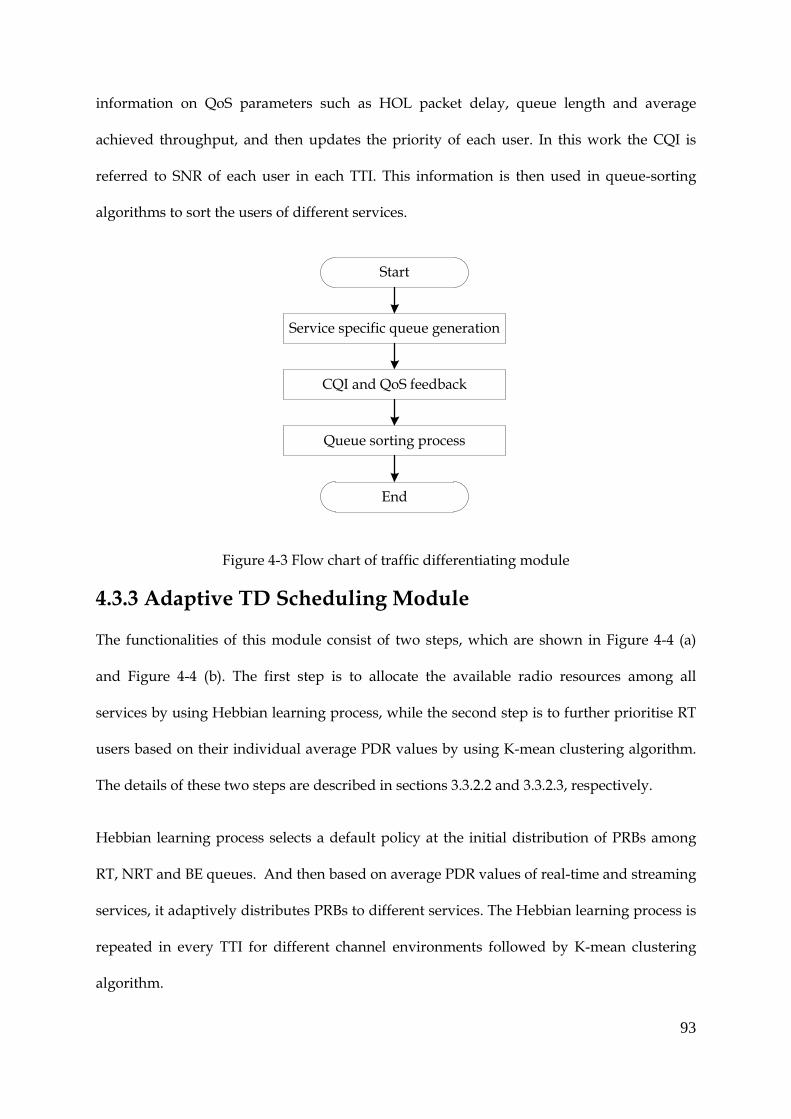
93
information on QoS parameters such as HOL packet delay, queue length and average
achieved throughput, and then updates the priority of each user. In this work the CQI is
referred to SNR of each user in each TTI. This information is then used in queue-sorting
algorithms to sort the users of different services.
Start
Service specific queue generation
CQI and QoS feedback
Queue sorting process
End
Figure 4-3 Flow chart of traffic differentiating module
Adaptive TD Scheduling Module 4.3.3
The functionalities of this module consist of two steps, which are shown in Figure 4-4 (a)
and Figure 4-4 (b). The first step is to allocate the available radio resources among all
services by using Hebbian learning process, while the second step is to further prioritise RT
users based on their individual average PDR values by using K-mean clustering algorithm.
The details of these two steps are described in sections 3.3.2.2 and 3.3.2.3, respectively.
Hebbian learning process selects a default policy at the initial distribution of PRBs among
RT, NRT and BE queues. And then based on average PDR values of real-time and streaming
services, it adaptively distributes PRBs to different services. The Hebbian learning process is
repeated in every TTI for different channel environments followed by K-mean clustering
algorithm.

94
Start
PDR Feedback for real-time & Streaming Services
Resource Allocation Decision
End
Initialise Default Policy
Figure 4-4(a) Flow chart of Hebbian learning module
The systematic flow of second step is shown in Figure 4-4 (b). The K-mean clustering
algorithm uses information of average PDR values of all RT users at individual user-level
instead of average PDR of overall real-time service (as in 4-4 a). This information is used as
an input vector for K-mean Clustering Algorithm to further prioritise RT user. Users with
similar average PDR are grouped together and then these groups in the next TTI are sorted
to give priority to the users with higher average PDR values.
Start
PDR Calculation of each RT User
Re-arrange Priority of RT users
End
K-Mean Clustering Algorithm
Figure 4-4(b) Flow chart of K-mean clustering module

95
Resource Allocation Module 4.3.4
A systematic flow of resource allocation module is shown in Figure 4-5. The output of
adaptive TD scheduler is a queue of users with set priorities. These users are allocated PRBs
in the resource allocation module. This module picks users one-by-one based on their
priority order and allocates PRBs to the users by exploiting FD MU diversity. After
allocating PRBs, it calculates throughput of each user, system throughput and QoS provided
to each user.
Start
CQI Feedback
PRB/Sub channel Allocation
QoS Measurements
End
User Selection
Throughput Calculation
Figure 4-5 Flow chart of resource allocation module
Feedback Module 4.3.5
The flow process of feedback module is shown in Figure 4-6. This module calculates the user
SNR in each PRB, throughput of all NRT users, HOL packet delay and average PDR of RT
users. It then sends this information to Traffic Differentiator stage and adaptive TD Scheduler
stage. The information on SNR, throughput and delay is sent to Traffic Differentiator stage;
meanwhile the information of average PDR of real-time service and individual average PDR

96
of RT users is sent to TD Scheduler stage. In addition, SNR information on each PRB will be
also fed to the FD Scheduler stage.
Start
Calculate SNR on each PRB
Send feedback
End
Calculate Average PDR of RT traffic and Individual RT users
Figure 4-6 Flow chart of feedback module
Wireless Channel Model 4.4
For the design of a radio communication system the information about radio communication
channel characteristics is very important. Unlike fixed communication systems, the
environment of wireless mobile communication systems is difficult to predict. Traditionally,
radio channels are modelled in a statistical way using real propagation measurement data.
Many measurements and studies have been done to obtain the characteristics of the radio
environment. A good review of these measurements is given in [APY95] [FL96] [Mokdarl91]
and [Hashmi93]. In general, signal fading in a radio environment can be divided into three
components: a large-scale path loss, a medium-scale slow varying, and a small-scale fast
fading. Accordingly, these three propagation components are used to describe a wireless
environment that consists of path loss, shadowing (also called slow fading), and multipath
(also called fast fading).

97
Figure 4-7 illustrates the three propagation phenomena occurring in wireless scenario.
Figure 4-7 Radio channel attenuation
Path loss is phenomena of decreasing received signal power with distance due to reflection,
diffraction around structures, and refraction with them. Shadowing is caused by obstruction
of buildings, hills, trees, and foliage. Multipath fading is due to multipath reflection of a
transmitted signal by objects like house, building, and other man-made structures, or
natural objects such as forests surrounding a mobile unit.
In the large-scale transmission model path loss and shadow fading are influenced by the
slow changes of average signal power and UEs positions. Meanwhile, in the small-scale
transmission model multipath fading is mainly caused by the reflection, refraction and
diffraction due to UEs movement and obstacles in the environment. It is used to describe
fast change in the signal strength in short distances or short time.
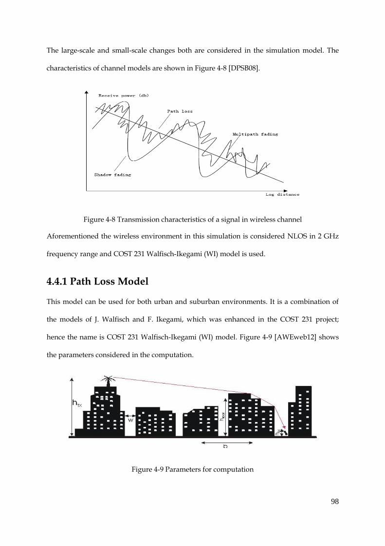
98
The large-scale and small-scale changes both are considered in the simulation model. The
characteristics of channel models are shown in Figure 4-8 [DPSB08].
Figure 4-8 Transmission characteristics of a signal in wireless channel
Aforementioned the wireless environment in this simulation is considered NLOS in 2 GHz
frequency range and COST 231 Walfisch-Ikegami (WI) model is used.
Path Loss Model 4.4.1
This model can be used for both urban and suburban environments. It is a combination of
the models of J. Walfisch and F. Ikegami, which was enhanced in the COST 231 project;
hence the name is COST 231 Walfisch-Ikegami (WI) model. Figure 4-9 [AWEweb12] shows
the parameters considered in the computation.
Figure 4-9 Parameters for computation

99
The model considers the buildings in the vertical plan between the transmitter (Tx) and the
receive (Rx), in which street widths, building heights, transmitter and receiver heights are
considered.
The accuracy of this model is quite high because in urban environments, the propagation in
the vertical plan and over the rooftops i.e. multiple diffraction is dominating, especially if
the transmitters are mounted above rooftop levels [AWEweb12].
The general parameters of the model are:
Frequency (f): (800 to 2000MHz)
Height of transmitter : (4 to 50 m)
Height of the receiver : (1 to 3 m)
Distance d between the transmitter and receiver: (20 to 5000 m)
The parameters depending on buildings are:
Mean value of building heights:
Mean value of width of streets: W
Mean value of building separation: b
There are three terms which make up this path loss model [EHSB01].
(4-1)
= Free space loss
= Roof top to street diffraction

100
= Multi-screen loss
Free space loss is calculated as:
( ) ( ) (4-2)
In which, D is the distance of user from eNB measured in km and f is the carrier frequency
measured in MHz.
Roof top to street diffraction is calculated as:
( ) ( ) ( ) (4-3
In which,
(4-4)
In which and represent building height, Mobile Station (MS) height
and the difference between building and MS heights measured in meters. And w is street
width, which is also measured in meters.
The multi-screen loss is calculated as:
( ) ( ) ( ) (4-5)
In which,
( ( )) (4-5)
( (
)) (4-6)
In which b is the building spacing measured in meters.

101
The value of b=60 m, w = 12 m, average height of roof is 25 m, average mobile height is 1.5 m
and average eNB height is 40 m.
Shadow Fading Model 4.4.2
The correlation for shadow fading is defined as [3GPP09b]:
Shadowing correlation={ ( )
( ) (4-7)
Shadow fading ⁄ (4-8)
In which, is lognormal Gaussian distribution of user k such as:
and (4-9)
In which, and are two Gaussian random variables with an expectation 0 and standard
deviation 8 dB. In addition, a and b are amplitudes of the real and imaginary parts of the
signal, respectively. When , the correlation is 50% and when , the
correlation is 100%.
Multipath Fading 4.4.3
Multipath fading or fast fading or multipath is an important character of wireless channel.
When a radio signal is reflected or refracted in the transmission medium, they arrive at the
receiver with more than one path. If the arrival time and the phase of the multiple signals
are different then these signals can interfere constructively or destructively with each other
at the receiver and the amplitude of resultant signal at the receiver changes dynamically.
This scenario is called fast fading [TV05].
Rayleigh fading model is used in this simulation as it is suitable for NLOS urban
environment. A complex number is used to express the amplitude and phase characteristics

102
of the wireless channel. The real and imaginary parts of this complex number, MF=a + b*i
are two Gaussian random variables with expectation 0 and standard deviation 1.
Radio Resource Allocation 4.5
Radio resource allocation in OFDMA-based LTE-A networks considers available spectrum
resources both in time and frequency domains. Its aim is to effectively use spectrum
resources and improve the network performance. The basic resource allocation unit in LTE-
A network is PRB and one PRB is allocated to one user in the DL scheduling.
Let the total bandwidth be B, the total number of subcarriers be N, the bandwidth for each
subcarrier be ∆ƒ which is equal to 15 kHz and one PRB is composed of 12 subcarriers. There
are K users in the system and each user has data rate requirement .
According to Shannon theory, the data rate is defined as a function of SNR and it can be
expressed as,
( ) (4-9)
In which, f is the PRB bandwidth, is SNR of user k on RB m.
Based on Section 4.3, the wireless channel power gain for user k on subcarrier n experiences
the path loss, shadowing fading and multipath fading. This can be expressed as,
[ ] (4-10)
For user k, let the power transmitted on subcarrier n be and be the variance of
AWGN on subcarrier n then the SNR for user k on this subcarrier is:
[ ]
(4-11)

103
Since the scheduling unit is PRB, let the transmission power on all PRBs be the same which
is given as,
where M is total number of PRBs, is the transmission power for
user k on PRB m. Let is the average SNR for user k on all the subcarriers in PRB m,
[ ] is the channel power gain for user k on PRB m i.e. the average channel power gain for
user k on all the subcarriers of PRB m. Then for user k, the data rate transmitted on PRB m is
given as:
( [ ]
) (4-12)
In which, L is number of consecutive subcarriers in a PRB.
Simulation Validation 4.6
The simulation model is an important groundwork of this thesis, so the simulation code is
debugged line by line. Each module is run separately and then the simulator is analysed and
validated by using classic scheduling algorithms such as RR, MAX C/I and PF in the Traffic
Differentiator stage, and fair or strict pre-scheduling algorithms at the TD Scheduler stage. For
this purpose three service queues are considered in which users are sorted by classic RR,
MAX C/I and PF algorithms, respectively. In each simulation equal number of users and
same network scenarios are taken into account to validate the results. The obtained results
are same with theoretic results defined in the classic algorithms. Theoretically, as explained
in Section 2.6, RR algorithm achieves the highest fairness level and the lowest system
throughput. MAX C/I algorithm, on the other hand achieves the highest system throughput
and the lowest fairness level. PF algorithm however makes a good trade-off between system
throughput and fairness level by achieving system throughput higher than RR algorithm
and fairness level higher than MAX C/I algorithm. The validation results consider system
throughput achieved by RR, MAX C/I and PF algorithm.

104
Random Distribution of UEs 4.6.1
In the first step of simulation the system parameters and cell topology are initialised. The
correlation between different network topologies is eliminated with random UE positions
and wireless channel initialisation process. The wireless channel gain is updated in each TTI.
In the simulation single cell topologies are used and the performance of all packet
scheduling algorithms is analysed under the same network conditions. Average results are
taken by running the simulation over a number of iterations under a particular scenario. The
radius of the cell is 1 km and all UEs are randomly distributed within the cell with minimum
distance of 35 m from eNB.
The position of eNB is (0, 0). The position of eNB and all UEs in one simulation topology is
shown in Figure 4-10 which shows the user random distribution characteristic.
Figure 4-10 UE positions when UE number is 50
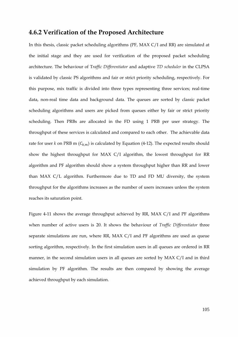
105
Verification of the Proposed Architecture 4.6.2
In this thesis, classic packet scheduling algorithms (PF, MAX C/I and RR) are simulated at
the initial stage and they are used for verification of the proposed packet scheduling
architecture. The behaviour of Traffic Differentiator and adaptive TD scheduler in the CLPSA
is validated by classic PS algorithms and fair or strict priority scheduling, respectively. For
this purpose, mix traffic is divided into three types representing three services; real-time
data, non-real time data and background data. The queues are sorted by classic packet
scheduling algorithms and users are picked from queues either by fair or strict priority
scheduling. Then PRBs are allocated in the FD using 1 PRB per user strategy. The
throughput of these services is calculated and compared to each other. The achievable data
rate for user k on PRB m ( ) is calculated by Equation (4-12). The expected results should
show the highest throughput for MAX C/I algorithm, the lowest throughput for RR
algorithm and PF algorithm should show a system throughput higher than RR and lower
than MAX C/L algorithm. Furthermore due to TD and FD MU diversity, the system
throughput for the algorithms increases as the number of users increases unless the system
reaches its saturation point.
Figure 4-11 shows the average throughput achieved by RR, MAX C/I and PF algorithms
when number of active users is 20. It shows the behaviour of Traffic Differentiator three
separate simulations are run, where RR, MAX C/I and PF algorithms are used as queue
sorting algorithm, respectively. In the first simulation users in all queues are ordered in RR
manner, in the second simulation users in all queues are sorted by MAX C/I and in third
simulation by PF algorithm. The results are then compared by showing the average
achieved throughput by each simulation.
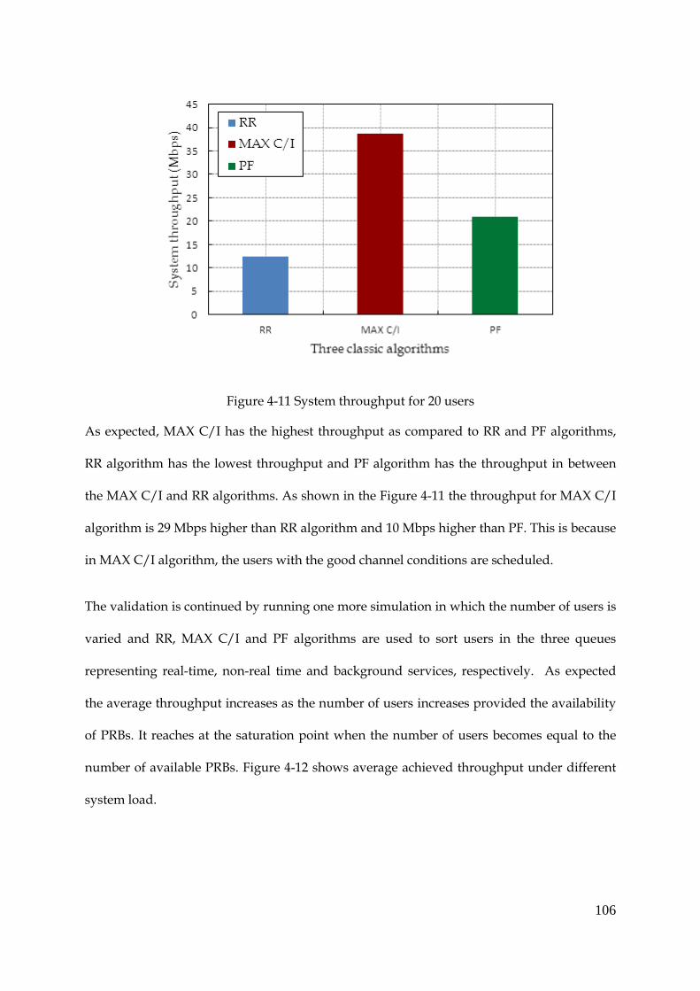
106
Figure 4-11 System throughput for 20 users
As expected, MAX C/I has the highest throughput as compared to RR and PF algorithms,
RR algorithm has the lowest throughput and PF algorithm has the throughput in between
the MAX C/I and RR algorithms. As shown in the Figure 4-11 the throughput for MAX C/I
algorithm is 29 Mbps higher than RR algorithm and 10 Mbps higher than PF. This is because
in MAX C/I algorithm, the users with the good channel conditions are scheduled.
The validation is continued by running one more simulation in which the number of users is
varied and RR, MAX C/I and PF algorithms are used to sort users in the three queues
representing real-time, non-real time and background services, respectively. As expected
the average throughput increases as the number of users increases provided the availability
of PRBs. It reaches at the saturation point when the number of users becomes equal to the
number of available PRBs. Figure 4-12 shows average achieved throughput under different
system load.
107
Figure 4-12 System throughput for different number of active users
It is shown that by increasing number of users, system throughput increases unless users are
more than the number of PRBs and system reaches the saturation point.
The validation is also conducted by taking the throughput of users at TTI level so that
instantaneous throughput of users can be analysed to validate the random changes in user
positions and network conditions. The example of the instantaneous throughput of users
along number of TTIs is shown in Figure 4-13.

108
Figure 4-13 System instantaneous throughput
Figure 4-13 shows instantaneous throughput of 70 users at each TTI when 100 number of
TTIs are used, which varies randomly due to time varying wireless channel conditions and
changing positions of users. For system level throughout, instantaneous throughput on all
TTIs is added and averaged over number of total active users.
Verification of the Number of Iterations 4.6.3
The number of simulation iterations impacts the simulation results a lot. This is because the
locations of users will change randomly in each simulation loop and wireless channel
conditions are time variant. To combat the effect of randomness and of time variant
characteristics of channel conditions, large number of TTI is recommended, for proper
simulation results.
From simulation point of view, the higher the number of simulation iteration, the longer the
simulation time. Therefore a verification of deciding a reasonable number of iterations for
simulations is required. Therefore average system throughput is calculated with different
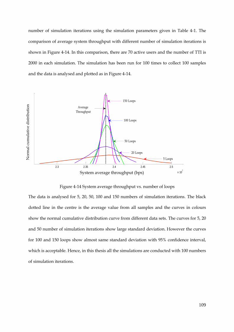
109
number of simulation iterations using the simulation parameters given in Table 4-1. The
comparison of average system throughput with different number of simulation iterations is
shown in Figure 4-14. In this comparison, there are 70 active users and the number of TTI is
2000 in each simulation. The simulation has been run for 100 times to collect 100 samples
and the data is analysed and plotted as in Figure 4-14.
Figure 4-14 System average throughput vs. number of loops
The data is analysed for 5, 20, 50, 100 and 150 numbers of simulation iterations. The black
dotted line in the centre is the average value from all samples and the curves in colours
show the normal cumulative distribution curve from different data sets. The curves for 5, 20
and 50 number of simulation iterations show large standard deviation. However the curves
for 100 and 150 loops show almost same standard deviation with 95% confidence interval,
which is acceptable. Hence, in this thesis all the simulations are conducted with 100 numbers
of simulation iterations.
2.3 2.35 2.4 2.45 2.5
x 107System average throughput (b/s)
50 Loops
20 Loops
150 Loops
100 Loops
Average
Throughput
5 Loops
System average throughput (bps)
No
rmal
cu
mu
lati
ve
dis
trib
uti
on
110
Summary 4.7
In this chapter the system-level simulation set up is presented, which is used to analyse the
performance of packet scheduling architecture. The overall flow chart and the detailed
modules are described. Simulation parameters, wireless channel model and radio resource
allocation model are also presented in this chapter. In addition, simulation validation and
verification of number of iterations is presented. Simulation results on all algorithms
including SSSA, Hebbian learning and K-mean and the joint performance of all algorithms
are given in the next chapter.

111
Chapter 5 Simulation Results and Analysis
This chapter shows the simulation results and their analysis from different perspectives, to
evaluate the performance of the proposed scheduling architecture. These results show the
performance improvements of the proposed, SSSA, Hebbian learning process, K-mean
clustering algorithms separately and the performance of overall scheduling architecture. The
performance of overall scheduling architecture is tested under different network scenarios
such as changing traffic split among real-time, streaming and background services and by
varying system load, to exemplify the real network.
The results are compared against state-of-the-art QoS aware Mixed Traffic Packet
Scheduling algorithm in UTRAN Long Term Evolution Downlink (abbreviated as MIX)
[JNTMM08], Sum Waiting Based Scheduling (SWBS) [SYLX09] and classic PF algorithm. In
MIX [JNTMM08], mix traffic is differentiated into service queue, conventional algorithms
including PF and MAX C/I are used to sort users in the queues of different services and in
the TD, fair scheduling methods are used to pick users from the queues. The second
reference algorithm SWBS [SYLX09] uses the sum of waiting time of all packets of real-time
and non-real time services, respectively to prioritise users in the queues. Waiting time for
real-time service is the time during which packets remain in the queue to be scheduled and
for non-real time service it is calculated by considering the throughput requirements of this
service (section 2.6.4). Users maximising the product of sum waiting time and channel gain
(Equation 2-7) are prioritised. While in the proposed architecture CLPSA, novel service-
specific queue-sorting algorithms (SSSA) are used to prioritise users in RT and NRT queues,
the conventional PF algorithm is used for BE queue and FCFS is used for the control data
queue. In the TD, the scheduling architecture uses novel ATDSA to allocate radio resource
112
efficiently to the prioritised users in RT, NRT and BE queues. In the FD Scheduler stage, PRBs
are mapped to the selected users by M-PF algorithm.
Traffic Model 5.1
An ON-OFF source is used to generate packets for real-time voice service, streaming video
service and background service. It uses only two states, i.e. ON and OFF states and the time
spend between these two states is referred as transition time. The transition time is expected
to follow an exponential distribution [Adas97]. For each user, the source generates packets at
constant rate. The ON-OFF source is characterised by L, which is the mean number of
packets generated during the ON time, the peak rate during ON time S and the mean rate of
total ON and OFF time r. These factors determine the mean duration of the ON and OFF
states. The equilibrium probability of the ON state of the source is calculated as, φ=r/S. As
the ON and OFF states are exponentially distributed, the source can be modelled by two-
state Markov chain. The mean packet generation rate during ON time is represented by L
and is assumed to be much greater than 1, i.e. L >> 1. The transition probabilities are
represented by x and y. The transition rates of the source from ON to OFF and vice versa, is
calculated as follows [Chandrasekaran06]:
( ) ( ( ))⁄ (5-1)
As, , which basically means ( ) therefore ( ). Substituting value
of “ ” in (5-1),
( ) (5-2)
Or, ( )⁄ (5-3)
( ) ⁄ (5-4)

113
Substituting value of “S” in (5-4),
( )
(5.5)
Or, ( )⁄ (5.6)
Therefore,
( )⁄ (5-7)
( )⁄ (5-8)
The probability of mean “ON” time is 0.35 and the user remains active for 0.1 second in the
“ON” time. The packets are generated at constant rate, which is 3 packets in every “ON”
time for real-time service, 2 packets for non-real time streaming video service and 1 packet
for background service [Chandrasekaran06].
The ON-OFF source is shown in Figure 5-1[Chandrasekaran06].
Figure 5-1 ON-OFF traffic model
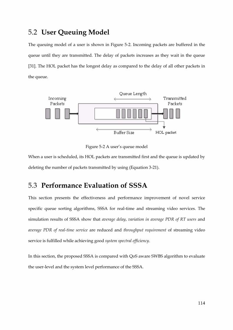
114
User Queuing Model 5.2
The queuing model of a user is shown in Figure 5-2. Incoming packets are buffered in the
queue until they are transmitted. The delay of packets increases as they wait in the queue
[31]. The HOL packet has the longest delay as compared to the delay of all other packets in
the queue.
Figure 5-2 A user’s queue model
When a user is scheduled, its HOL packets are transmitted first and the queue is updated by
deleting the number of packets transmitted by using (Equation 3-21).
Performance Evaluation of SSSA 5.3
This section presents the effectiveness and performance improvement of novel service
specific queue sorting algorithms, SSSA for real-time and streaming video services. The
simulation results of SSSA show that average delay, variation in average PDR of RT users and
average PDR of real-time service are reduced and throughput requirement of streaming video
service is fulfilled while achieving good system spectral efficiency.
In this section, the proposed SSSA is compared with QoS aware SWBS algorithm to evaluate
the user-level and the system level performance of the SSSA.

115
The system model of simulations in this section is shown in Figure 5-3.
Mixed Traffic
Traffic Differentiation
RT Queue Sorting Algorithm
NRT Queue Sorting Algorithm
Time Domain Fair Scheduling
Frequency Domain Resource Allocation
ATDSA is not IncorporatedBE Queue Sorting using PF Algorithm
Figure 5-3 System model of SSSA
The input is mix traffic, which is differentiated into queues based on the requirements of
users. Users in the RT queue and NRT queue are prioritised by the novel SSSA, users in the
BE queue are prioritised by conventional PF algorithm and control data packets are
transmitted in FCFS manner. The prioritised users are then picked one-by-one using fair
scheduling in the TD and finally allocated PRBs in the FD using M-PF algorithm. Novel
ATDSA, which is proposed in the TD to intelligently distribute the available PRBs among all
services, is not implemented in these results. This is because this section presents the
effectiveness of SSSA, separately.
QoS Performance of Real Time and Streaming Services 5.3.1
QoS of real-time service is evaluated by average delay and average PDR of real-time service
and average PDR variation of RT users. QoS of non-real time service is evaluated by average

116
achieved throughput of streaming video service. The average achieved throughput of background
service is also presented in this section.
The number of RT users is taken equal to the total number of NRT and BE users
representing equal load from real-time and non-real time services, as used in [SYLX09].
Figure 5-4 shows the average delay of real-time service for SSSA and SWBS algorithms with
system load.
Figure 5-4 Average delay of real-time service
The proposed SSSA shows slightly higher delay than the reference SWBS algorithm up to a
load of 80 active users however, which becomes lower than SWBS at system loads higher
than 80 active users. This is because the proposed SSSA considers QSI in terms of queue
length of users, to prioritise RT users. Queues do not build up at lower system loads, where
packets of all users are scheduled. At higher system loads when competition to get radio
resource is high, each user’s queue becomes longer and longer. In this scenario, the
consideration of queue length in queue-sorting becomes effective and lowers the average
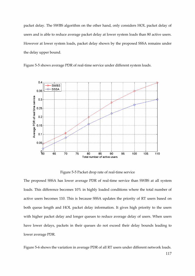
117
packet delay. The SWBS algorithm on the other hand, only considers HOL packet delay of
users and is able to reduce average packet delay at lower system loads than 80 active users.
However at lower system loads, packet delay shown by the proposed SSSA remains under
the delay upper bound.
Figure 5-5 shows average PDR of real-time service under different system loads.
Figure 5-5 Packet drop rate of real-time service
The proposed SSSA has lower average PDR of real-time service than SWBS at all system
loads. This difference becomes 10% in highly loaded conditions where the total number of
active users becomes 110. This is because SSSA updates the priority of RT users based on
both queue length and HOL packet delay information. It gives high priority to the users
with higher packet delay and longer queues to reduce average delay of users. When users
have lower delays, packets in their queues do not exceed their delay bounds leading to
lower average PDR.
Figure 5-6 shows the variation in average PDR of all RT users under different network loads.
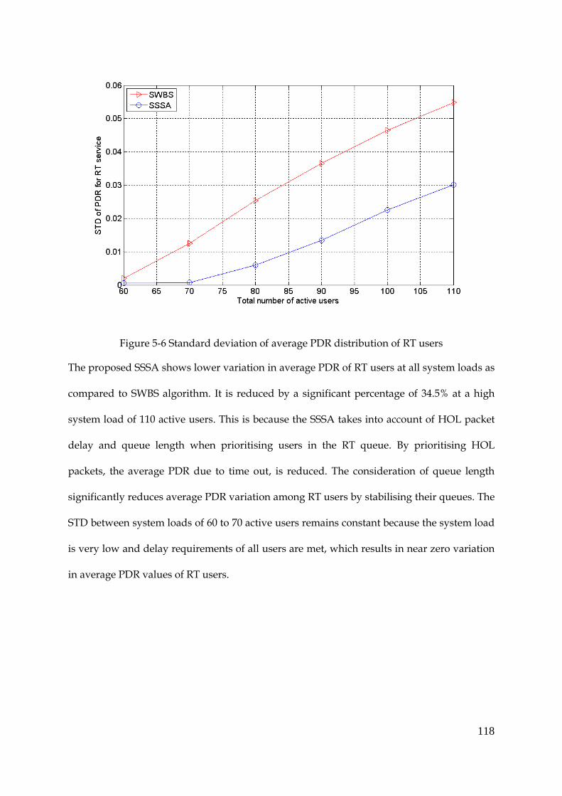
118
Figure 5-6 Standard deviation of average PDR distribution of RT users
The proposed SSSA shows lower variation in average PDR of RT users at all system loads as
compared to SWBS algorithm. It is reduced by a significant percentage of 34.5% at a high
system load of 110 active users. This is because the SSSA takes into account of HOL packet
delay and queue length when prioritising users in the RT queue. By prioritising HOL
packets, the average PDR due to time out, is reduced. The consideration of queue length
significantly reduces average PDR variation among RT users by stabilising their queues. The
STD between system loads of 60 to 70 active users remains constant because the system load
is very low and delay requirements of all users are met, which results in near zero variation
in average PDR values of RT users.

119
Figure 5-7 shows the average throughput of streaming service achieved by the proposed
SSSA and SWBS under different system loads.
Figure 5-7 Average achieved throughput of streaming service
Both the proposed SSSA and SWBS algorithm meet throughput requirement of streaming
service (240 kbps) at all system loads. However SSSA achieves slightly lower throughput
than SWBS because it allocates sufficient resources to streaming and real-time services based
on their QoS requirements and the rest to the background service, to prevent any starvation.
SWBS does not differentiate between streaming and background services and treats them
equally, which may results in either over allocation or starvation to background service.
The results on average achieved throughput by background service are also presented to
verify that BE queue does not starve forever. This is the particular issue to be considered in
communication systems, especially in LTE-A, which has diverse range of applications. Most
of the current scheduling algorithms do not consider separately the background service
while focusing on services with QoS requirements. That is why these algorithms either over

120
allocate the background service or cause starvation to it. Although background service does
not have QoS requirement but still it should not starve forever.
Figure 5-8 shows average achieved throughput of background service shown by SSSA and
SWBS under different system loads.
Figure 5-8 Average throughput of background service
The proposed SSSA shows lower throughput as compared to SWBS and the difference
becomes higher when the system is highly loaded. This is because SSSA considers streaming
and background as two separate services and tries to fulfil the minimum required
throughput to streaming service first. SWBS however equally considers both services and
achieves the average throughput of both at equal level. In this way it over allocates the BE
queue and as a result cannot keep delay, delay variation and average PDR of real-time
service lower, especially when system load is high. The proposed SSSA allocates resources
to BE queue after considering QoS of RT and NRT queues.

121
System Performance 5.3.2
System performance is analysed by calculating fairness among users and overall system
throughput. Fairness among users is calculated by Equation 3-24.
Figure 5-9 shows fairness achieved by the proposed SSSA, QoS aware SWBS algorithm and
classic PF algorithm under different system loads.
Figure 5-9 Fairness among all users
The proposed SSSA achieves higher fairness at all system loads, as compared to SWBS. This
is because SSSA adaptively allocates resources to each queue and tries to prevent over
allocation or starvation to any service. SWBS over allocates some services and cannot
achieve good fairness. This is achieved by updating the priorities of users in each queue
before scheduling decisions. The fairness results are also compared with classic PF
algorithm, which is considered as a bench mark for a good trade-off between system
throughput and user fairness. The proposed SSSA shows almost same fairness with PF at
lower system loads from 60 to 70 active users because every user can get radio resource. At

122
system load higher than 70 active users, fairness shown by SSSA becomes slightly lower
than PF algorithm. This is because SSSA considers both user-level and system-level
performance and PF algorithm considers only system-level performance.
Figure 5-10 System spectral efficiency
Figure 5-10 shows system throughput achieved by the proposed QoS aware SSSA, SWBS
and conventional PF algorithms under different system loads. The proposed SSSA
outperforms all other algorithms. It improves overall system throughput by 4.35 Mbps at a
system load of 100 active users, as compared to SWBS and MIX. This is because SSSA takes
into account of both TD and FD MU diversity by considering radio channel conditions. It
also shows good system throughput than classic PF algorithm, which considers both fairness
and system throughput equally to make the best trade-off between them. QoS aware SWBS
however shows lower throughput than PF algorithm up to a load of 90 active users and
increases afterwards due to exploiting MU diversity in TD. As PF algorithm does not only
improve system throughput but makes a balance between system throughput and user
fairness and shows lower throughput than SWBS at higher system loads.

123
These results show that the proposed SSSA makes a better trade-off between user-level and
system-level performance, as compared to SWBS and PF algorithms. SSSA meets the
minimum throughput requirement of NRT traffic, and also reduces the average PDR
variation in average PDR of RT users, average delay and average PDR of real-time service
by sacrificing throughput of background service slightly. Meanwhile it maintains good
system-level performance by improving system throughput and user fairness.
Joint (SSSA & ATDSA) Performance Evaluation 5.4
This thesis proposes a novel adaptive time domain scheduling algorithm (ATDSA), to
allocate sufficient resources to real-time and streaming video service to meet their QoS
requirements and allocate rest of the resource to background service, to maintain fairness
among users of all services. Hebbian learning process is integrated in ATDSA to intelligently
allocate available resources to different services. In addition K-mean clustering algorithm is
used to further reduce average PDR of real-time service and the average PDR variation
among RT users.
The joint results of the proposed SSSA and ATDSA are presented under different network
scenarios. This is to validate the credibility of the proposed architecture under real network
conditions. The focus of this research work is to improve the QoS of real-time voice and non-
real time streaming video services while maintaining the overall system-level performance
in terms system throughput and user fairness. Therefore, the simulation results include
average packet delay, variation in average PDR of RT users and average PDR of real-time service,
minimum throughput of non-real time service, system throughput and user fairness.
The performance of the proposed ATDSA is compared against two recent QoS aware MIX
[JNTMM08] and SWBS algorithms [SYLX09].

124
The system model used in this section is shown in Figure 5-11.
Figure 5-11 System model of CLPSA
It considers all proposed algorithms at different stages of CLPSA, which include SSSA at the
Traffic Differentiator, ATDSA at the TD Scheduler and M-PF at the FD Scheduler stage.
To exemplify real network, the performance of the proposed scheduling architecture
CLPSA is evaluated under the following simulation scenarios.
Scenario 1: Equal distribution of real-time and non-real time services.
(Real-time service 50%, streaming service 25%, Background service 25%)
Scenario 2: Real-time service dominant over other services.
(Real-time service 70%, streaming service 20%, Background service 10%)
Scenario 3: Background service dominant over other services.
(Real-time service 20%, streaming service 20%, Background service 60%)
Scenario 4: Streaming service dominant over other services.
(Real-time service 20%, streaming service 70%, Background service 10%)

125
Scenario 1: Equal Distribution of Real Time and Non 5.4.1
Real time Services
In this scenario, real-time service is 50%, streaming service is 25% and background service is
25% of the total system load. The performance of the proposed scheduling architecture is
represented by CLPSA, which is compared with SWBS and MIX.
Figure 5-12 shows average packet delay for the proposed CLPSA and the reference (MIX
and SWBS) algorithms under different system loads.
Figure 5-12 Average packet delay of real-time service
As expected, average packet delay of real-time service for all algorithms increases with the
number of active users however the proposed CLPSA shows the lowest delay. This is
because CLPSA uses a novel delay-dependent queue-sorting algorithm for real-time service,
which prioritises users with higher HOL packet delay and longer queues. It uses novel
ATDSA in the TD, which allocates resources to real-time service based on its QoS
requirement. It allocates sufficient resources to further reduce average packet delay. MIX
due to lack of service-specific queue-sorting and uses fair scheduling scheme in the TD,
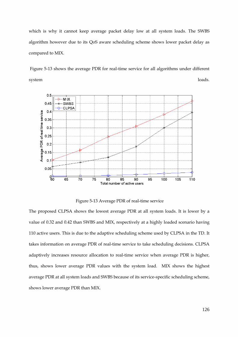
126
which is why it cannot keep average packet delay low at all system loads. The SWBS
algorithm however due to its QoS aware scheduling scheme shows lower packet delay as
compared to MIX.
Figure 5-13 shows the average PDR for real-time service for all algorithms under different
system loads.
Figure 5-13 Average PDR of real-time service
The proposed CLPSA shows the lowest average PDR at all system loads. It is lower by a
value of 0.32 and 0.42 than SWBS and MIX, respectively at a highly loaded scenario having
110 active users. This is due to the adaptive scheduling scheme used by CLPSA in the TD. It
takes information on average PDR of real-time service to take scheduling decisions. CLPSA
adaptively increases resource allocation to real-time service when average PDR is higher,
thus, shows lower average PDR values with the system load. MIX shows the highest
average PDR at all system loads and SWBS because of its service-specific scheduling scheme,
shows lower average PDR than MIX.
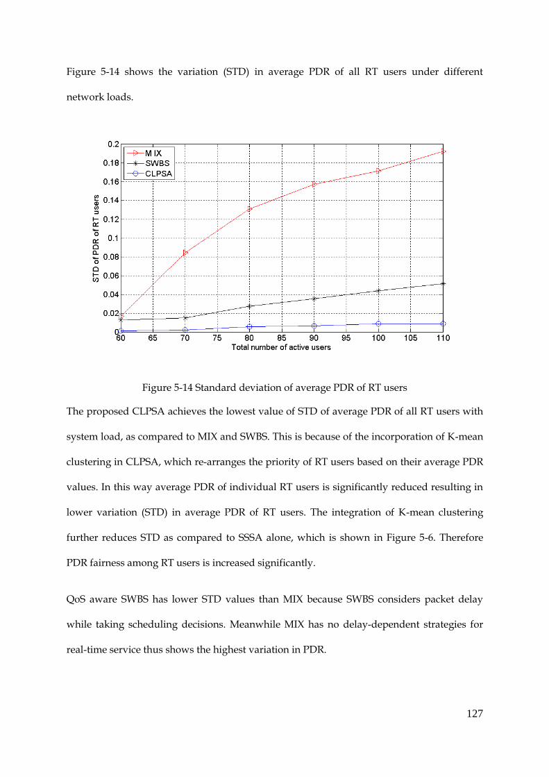
127
Figure 5-14 shows the variation (STD) in average PDR of all RT users under different
network loads.
Figure 5-14 Standard deviation of average PDR of RT users
The proposed CLPSA achieves the lowest value of STD of average PDR of all RT users with
system load, as compared to MIX and SWBS. This is because of the incorporation of K-mean
clustering in CLPSA, which re-arranges the priority of RT users based on their average PDR
values. In this way average PDR of individual RT users is significantly reduced resulting in
lower variation (STD) in average PDR of RT users. The integration of K-mean clustering
further reduces STD as compared to SSSA alone, which is shown in Figure 5-6. Therefore
PDR fairness among RT users is increased significantly.
QoS aware SWBS has lower STD values than MIX because SWBS considers packet delay
while taking scheduling decisions. Meanwhile MIX has no delay-dependent strategies for
real-time service thus shows the highest variation in PDR.

128
Figure 5-15 shows the average throughput of streaming service achieved by MIX, SWBS and
CLPSA algorithms with system load.
Figure 5-15 Average achieved throughput of streaming service
All algorithms achieve almost equal average achieved throughput up tp a system load of 80
active users. However when the load is further increased, the proposed CLPSA outperforms
SWBS and MIX algorithms, by achieving the highest throughout. This is because the
proposed CLPSA uses service specific queue-sorting algorithm SSSA for prioritising users
demanding streaming video service. The SSSA prioritises users with lower average achieved
throughput to improve QoS of NRT users. The adaptive scheduling algorithm in the TD,
ATDSA allocates sufficient resources to meet throughput requirement of streaming service.
However MIX due to its fair scheduling scheme in the TD cannot allocate resources to all
NRT users at higher system load therefore its average achieved throughput drops when
system load is higher than 90.

129
Figure 5-16 shows the fairness achieved by MIX, SWBS and the proposed CLPSA under
different system loads.
Figure 5-16 Fairness among all users
MIX due to its fair scheduling policy shows the highest fairness in this scenario where real-
time and non-real time services have equal load. The proposed CLPSA shows slightly lower
fairness than MIX, which is because CLPSA considers QoS of all services along with fairness.
SWBS however shows the lowest fairness because it only focuses on the QoS provision to
real-time and non-real time services. The good fairness index shown by the proposed
CLPSA is due to its particular design of allocating just enough resources to QoS demanding
services and the rest to background service. This is achieved by integrating Hebbian
learning process in CLPSA, which adaptively allocates sufficient radio resources to real-time
and streaming services and the rest to background service.
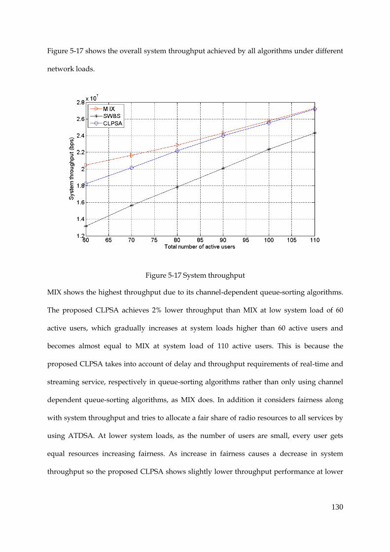
130
Figure 5-17 shows the overall system throughput achieved by all algorithms under different
network loads.
Figure 5-17 System throughput
MIX shows the highest throughput due to its channel-dependent queue-sorting algorithms.
The proposed CLPSA achieves 2% lower throughput than MIX at low system load of 60
active users, which gradually increases at system loads higher than 60 active users and
becomes almost equal to MIX at system load of 110 active users. This is because the
proposed CLPSA takes into account of delay and throughput requirements of real-time and
streaming service, respectively in queue-sorting algorithms rather than only using channel
dependent queue-sorting algorithms, as MIX does. In addition it considers fairness along
with system throughput and tries to allocate a fair share of radio resources to all services by
using ATDSA. At lower system loads, as the number of users are small, every user gets
equal resources increasing fairness. As increase in fairness causes a decrease in system
throughput so the proposed CLPSA shows slightly lower throughput performance at lower

131
system loads as compared to MIX. SWBS basically focuses QoS provision thus it achieves
lower system throughput as compared to both MIX and CLPSA.
Scenario 2: Real Time Service Dominant over Other 5.4.2
Services
In this scenario, real-time service is 70%, streaming video service is 20% and background
service is 10% of total system load.
Figure 5-18 shows average packet delay of real-time service under different system loads.
Figure 5-18 Average packet delay of real-time service
As expected, average packet delay increases for all algorithms with the system load however
the proposed CLPSA shows the lowest delay. This is because CLPSA uses delay-dependent
queue-sorting algorithm for real-time service, which prioritises users with higher HOL delay
and longer queues. Also CLPSA uses adaptive TD scheduling algorithms, which adaptively
allocates resources to different traffic types to meet their QoS requirements under changing
network conditions. SWBS shows almost similar packet delay to CLPSA at lower system

132
loads of 60 and 70 active users however the difference becomes higher at higher system
loads above 70 active users. MIX shows the highest packet delay out of all algorithms.
The average PDR of real-time service is shown in Figure 5-19 under different system loads.
Figure 5-19 Average PDR of real-time service
The proposed CLPSA shows the lowest average PDR values at all system loads because of
its adaptive scheduling policy, which takes information on average PDR of real-time service
before each scheduling decision. It increases resource allocation to real-time service when
average PDR becomes higher. MIX and SWBS have significantly higher average PDR than
CLPSA and it increases in a near linear way with system load. The reason is that MIX and
SWBS do not take into account of the information on average PDR of real-time service before
taking scheduling decisions and are not adaptive to the changing network scenarios.

133
Figure 5-20 shows STD of average PDR of all RT users under increasing system load.
Figure 5-20 Standard deviation of average PDR distribution of all RT users
The proposed CLPSA outperforms all reference algorithms by showing the lowest STD at all
system loads. This is because of K-mean clustering algorithm, which prioritises users with
higher average PDR values, thus, reducing the STD of average PDR distribution of all RT
users. However in this scenario where real-time service is dominant, STD shown by CLPSA
is slightly higher than STD achieved in the previous scenario where real-time and non-real
time services have equal load, as shown in Figure 5.13. This is because under this scenario
real-time service is the dominant. Mix shows the highest STD when compared with CLPSA
and SWBS. This is because MIX does not use service-specific queue-sorting and uses fair
scheduling to allocate radio resources to users demanding different services.

134
The average achieved throughput for streaming service is shown in Figure 5-21 for the
proposed CLPSA, SWBS and MIX.
Figure 5-21 Average achieved throughput of streaming service
All algorithms meet the throughput requirements of streaming video service because users
demanding this service are only 20% of whole active users in this scenario, where real-time
service is dominant over all other services. MIX however shows a sudden drop in average
achieved throughput at higher system loads because of its fair scheduling scheme. However
due to small number of users demanding streaming service, it can still meet minimum
throughput requirements at all system loads.
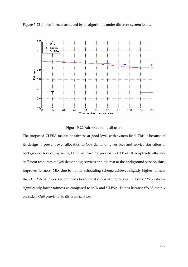
135
Figure 5-22 shows fairness achieved by all algorithms under different system loads.
Figure 5-22 Fairness among all users
The proposed CLPSA maintains fairness at good level with system load. This is because of
its design to prevent over allocation to QoS demanding services and service starvation of
background service, by using Hebbian learning process in CLPSA. It adaptively allocates
sufficient resources to QoS demanding services and the rest to the background service, thus,
improves fairness. MIX due to its fair scheduling scheme achieves slightly higher fairness
than CLPSA at lower system loads however it drops at higher system loads. SWBS shows
significantly lower fairness as compared to MIX and CLPSA. This is because SWBS mainly
considers QoS provision to different services.

136
Figure 5-23 shows the system throughput achieved by all algorithms under variable system
loads.
Figure 5-23 System throughput
The proposed CLPSA achieves almost similar system throughput at all system loads as
achieved by MIX, which uses channel dependent queue-sorting algorithms. At system loads
lower than 80 active users, CLPSA shows slightly lower system throughput, which is
because of considering both user-level and system-level performance at the same time.
However at system loads higher than 80 active users, CLPSA achieves higher system
throughput than MIX.
SWBS shows a nearly linear increase in system throughput with the system load, which is
lower than both MIX and CLPSA algorithms by a significant value of 60.18 Mbps at almost
all system loads.

137
Scenario 3: Background Service Dominant over Other 5.4.3
Services
In this scenario, the background service is 60%, real-time service is 20% and non-real time
service is 20% of total system load.
Figure 5-24 Average packet delay of real-time service
Figure 5-24 shows the comparison of the average packet delay of the real-time service
between the proposed CLPSA, MIX and SWBS algorithms with system load. The average
packet delay of the real-time service increases with the system load for these three
algorithms however, the proposed CLPSA shows the least packet delay. This is because
CLPSA uses delay-dependent queue-sorting algorithms for real-time service which
prioritises users with higher HOL packet delay and longer queues. Adaptive scheduling
with Hebbian learning process in ATDSA, allocates sufficient resources to real-time service
to meet its QoS requirement under this scenario as well. MIX shows the highest packet delay
with an average value of 0.44 ms at a system load of 110 active users. This is because MIX
lacks delay-dependent queue-sorting algorithms as used by CLPSA. SWBS shows lower
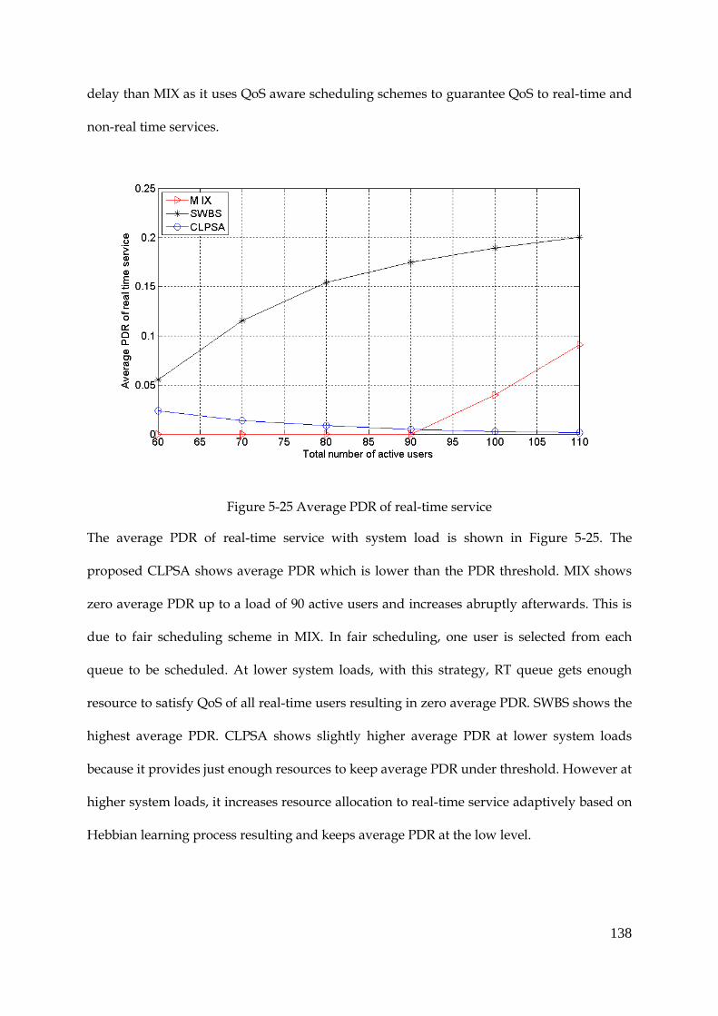
138
delay than MIX as it uses QoS aware scheduling schemes to guarantee QoS to real-time and
non-real time services.
Figure 5-25 Average PDR of real-time service
The average PDR of real-time service with system load is shown in Figure 5-25. The
proposed CLPSA shows average PDR which is lower than the PDR threshold. MIX shows
zero average PDR up to a load of 90 active users and increases abruptly afterwards. This is
due to fair scheduling scheme in MIX. In fair scheduling, one user is selected from each
queue to be scheduled. At lower system loads, with this strategy, RT queue gets enough
resource to satisfy QoS of all real-time users resulting in zero average PDR. SWBS shows the
highest average PDR. CLPSA shows slightly higher average PDR at lower system loads
because it provides just enough resources to keep average PDR under threshold. However at
higher system loads, it increases resource allocation to real-time service adaptively based on
Hebbian learning process resulting and keeps average PDR at the low level.

139
Figure 5-26 Standard deviation of average PDR distribution of all RT users
Figure 5-26 shows STD (variation) of average PDR of all RT users under different network
loads. For this scenario where real-time service is only 20% of the total load, all algorithms
show lower STD. However MIX shows zero STD value for system loads up to 100 active
users but it increases abruptly when load is further increased above 100 active users. This is
because MIX schedules users one-by-one from each queue and allocates a fair share of
resources to each traffic type. As in this particular scenario, the real-time users are only 20%
of all active users, thus with one-by-one scheduling policy up to a load of 100 active users,
all real-time users get enough resources in each TTI and hardly suffer any PDR. However at
higher system load, MIX is unable to schedule all real-time users resulting in a sudden
increase in average PDR, which is not the case with the proposed CLPSA. Although CLPSA
shows slightly higher STD than MIX at lower system loads but it maintains lower STD at
higher system loads as well. This is due to K-mean clustering algorithm, which prioritises
users with higher PDR values. In addition, the proposed CLPSA by using its adaptive
scheduling scheme allocates sufficient resources to real-time service at all system loads.
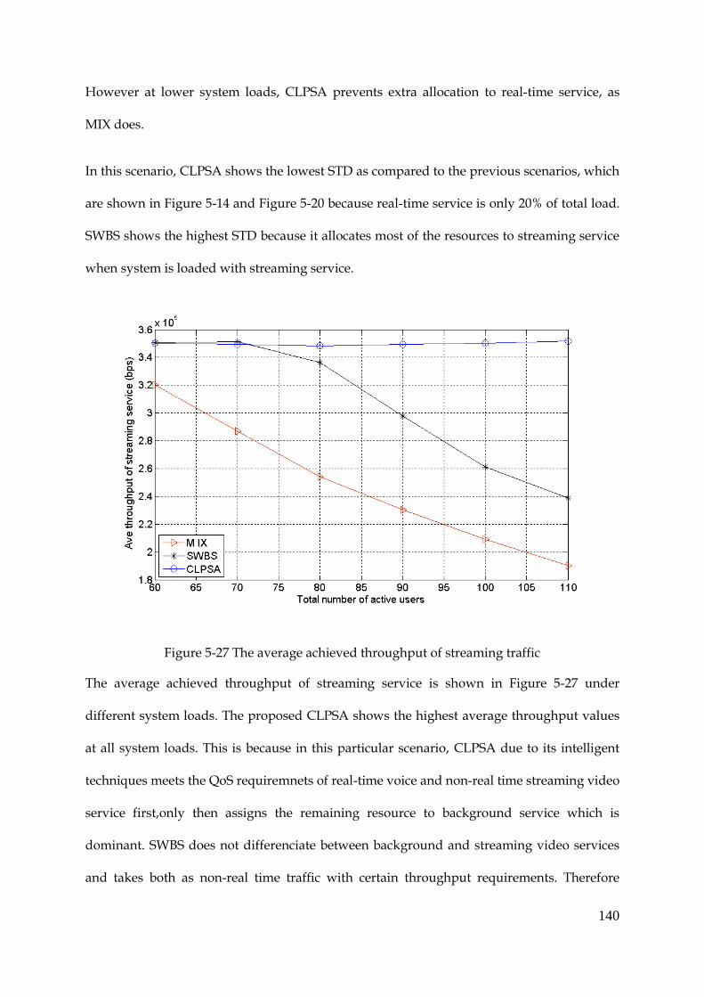
140
However at lower system loads, CLPSA prevents extra allocation to real-time service, as
MIX does.
In this scenario, CLPSA shows the lowest STD as compared to the previous scenarios, which
are shown in Figure 5-14 and Figure 5-20 because real-time service is only 20% of total load.
SWBS shows the highest STD because it allocates most of the resources to streaming service
when system is loaded with streaming service.
Figure 5-27 The average achieved throughput of streaming traffic
The average achieved throughput of streaming service is shown in Figure 5-27 under
different system loads. The proposed CLPSA shows the highest average throughput values
at all system loads. This is because in this particular scenario, CLPSA due to its intelligent
techniques meets the QoS requiremnets of real-time voice and non-real time streaming video
service first,only then assigns the remaining resource to background service which is
dominant. SWBS does not differenciate between background and streaming video services
and takes both as non-real time traffic with certain throughput requirements. Therefore
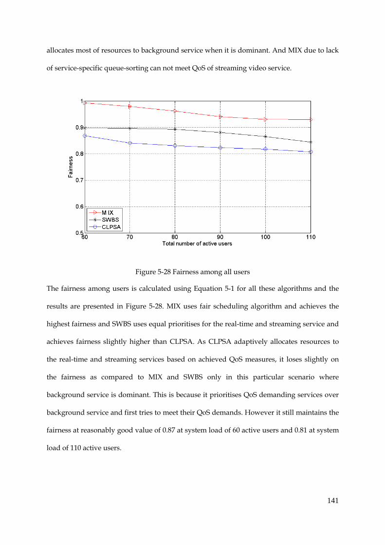
141
allocates most of resources to background service when it is dominant. And MIX due to lack
of service-specific queue-sorting can not meet QoS of streaming video service.
Figure 5-28 Fairness among all users
The fairness among users is calculated using Equation 5-1 for all these algorithms and the
results are presented in Figure 5-28. MIX uses fair scheduling algorithm and achieves the
highest fairness and SWBS uses equal prioritises for the real-time and streaming service and
achieves fairness slightly higher than CLPSA. As CLPSA adaptively allocates resources to
the real-time and streaming services based on achieved QoS measures, it loses slightly on
the fairness as compared to MIX and SWBS only in this particular scenario where
background service is dominant. This is because it prioritises QoS demanding services over
background service and first tries to meet their QoS demands. However it still maintains the
fairness at reasonably good value of 0.87 at system load of 60 active users and 0.81 at system
load of 110 active users.

142
Figure 5-29 System throughput
System throughput is the sum of throughput of all users and is shown in Figure 5-29 under
different system loads. MIX shows the highest throughput because it only uses channel
aware MAX C/I and PF as queue-sorting algorithms. SWBS shows good performance as
compared with the proposed CLPSA up to a system load of 95 active users and then
becomes lower than CLPSA. This is because SWBS does not consider streaming and
background service separately. The proposed CLPSA gives priority to voice and streaming
services as compared with background service. It only allocates resources to background
service when the throughput requirements of streaming service are met. As in this scenario
the background service is dominant, CLPSA shows slightly lower throughput than SWBS at
lower system loads from 60 to 95 active users however it becomes higher than SWBS at
higher system loads from 95 to 110.
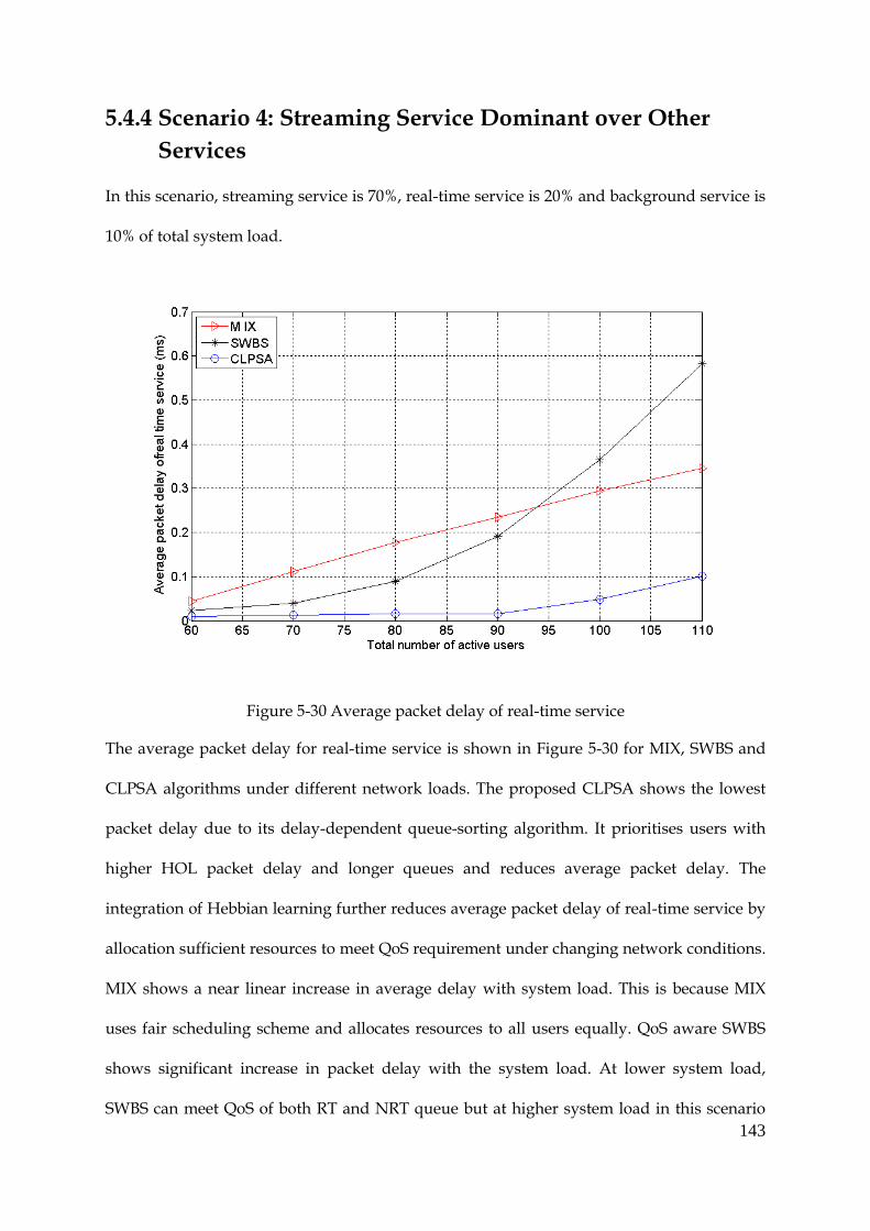
143
Scenario 4: Streaming Service Dominant over Other 5.4.4
Services
In this scenario, streaming service is 70%, real-time service is 20% and background service is
10% of total system load.
Figure 5-30 Average packet delay of real-time service
The average packet delay for real-time service is shown in Figure 5-30 for MIX, SWBS and
CLPSA algorithms under different network loads. The proposed CLPSA shows the lowest
packet delay due to its delay-dependent queue-sorting algorithm. It prioritises users with
higher HOL packet delay and longer queues and reduces average packet delay. The
integration of Hebbian learning further reduces average packet delay of real-time service by
allocation sufficient resources to meet QoS requirement under changing network conditions.
MIX shows a near linear increase in average delay with system load. This is because MIX
uses fair scheduling scheme and allocates resources to all users equally. QoS aware SWBS
shows significant increase in packet delay with the system load. At lower system load,
SWBS can meet QoS of both RT and NRT queue but at higher system load in this scenario
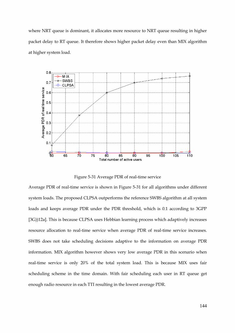
144
where NRT queue is dominant, it allocates more resource to NRT queue resulting in higher
packet delay to RT queue. It therefore shows higher packet delay even than MIX algorithm
at higher system load.
Figure 5-31 Average PDR of real-time service
Average PDR of real-time service is shown in Figure 5-31 for all algorithms under different
system loads. The proposed CLPSA outperforms the reference SWBS algorithm at all system
loads and keeps average PDR under the PDR threshold, which is 0.1 according to 3GPP
[3G))12a]. This is because CLPSA uses Hebbian learning process which adaptively increases
resource allocation to real-time service when average PDR of real-time service increases.
SWBS does not take scheduling decisions adaptive to the information on average PDR
information. MIX algorithm however shows very low average PDR in this scenario when
real-time service is only 20% of the total system load. This is because MIX uses fair
scheduling scheme in the time domain. With fair scheduling each user in RT queue get
enough radio resource in each TTI resulting in the lowest average PDR.

145
Figure 5-32 Standard deviation of average PDR distribution of RT users
Figure 5-32 shows STD of average PDR of all RT users with different network loads. As the
number of the real-time users in this scenario is only 20% of the total system load, all
algorithms have average PDR lower than the PDR threshold. Similar to scenario 3 where RT
users are 20% of the total system load, MIX shows the least STD up to a load of 100 active
users by its fair scheduling but cannot maintain it at higher system loads. The proposed
CLPSA however maintains STD at lower level at higher system load as well by intelligently
prioritising RT users.
MIX uses fair scheduling scheme and it has zero STD up to a load of 100 active users and it
increases suddenly afterwards. This is because it allocates resources to all users equally
without considering the changing load by different services. The proposed CLPSA considers
the changing network scenarios and takes scheduling decisions accordingly. It shows
slightly higher STD at lower system loads up to 104 active users however, it maintains STD
at lower level at higher system loads from 95 to 110 active users. This is because CLPSA
prioritises RT users based on the information of average PDR at the individual user-level, to
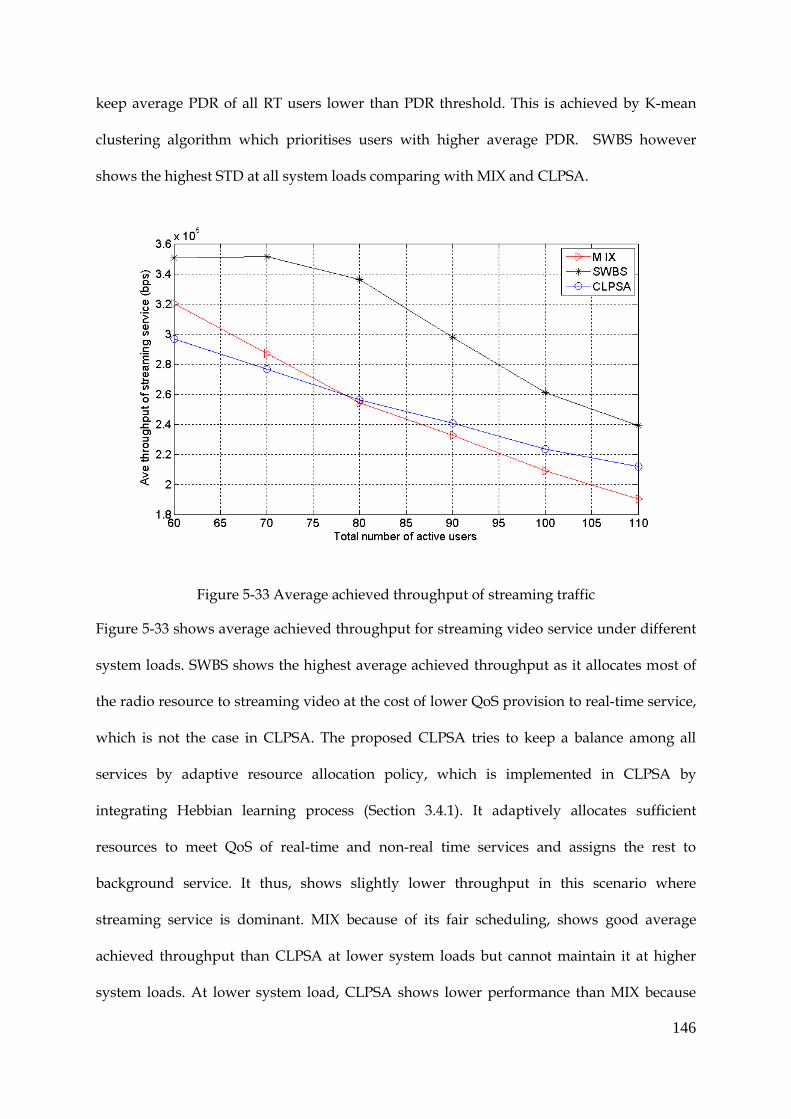
146
keep average PDR of all RT users lower than PDR threshold. This is achieved by K-mean
clustering algorithm which prioritises users with higher average PDR. SWBS however
shows the highest STD at all system loads comparing with MIX and CLPSA.
Figure 5-33 Average achieved throughput of streaming traffic
Figure 5-33 shows average achieved throughput for streaming video service under different
system loads. SWBS shows the highest average achieved throughput as it allocates most of
the radio resource to streaming video at the cost of lower QoS provision to real-time service,
which is not the case in CLPSA. The proposed CLPSA tries to keep a balance among all
services by adaptive resource allocation policy, which is implemented in CLPSA by
integrating Hebbian learning process (Section 3.4.1). It adaptively allocates sufficient
resources to meet QoS of real-time and non-real time services and assigns the rest to
background service. It thus, shows slightly lower throughput in this scenario where
streaming service is dominant. MIX because of its fair scheduling, shows good average
achieved throughput than CLPSA at lower system loads but cannot maintain it at higher
system loads. At lower system load, CLPSA shows lower performance than MIX because

147
CLPSA is designed to allocate just enough resource to meet QoS requirements. MIX
however is blind of QoS requirement and the changing network scenarios.
Figure 5-34 Fairness among all users
The fairness index achieved by MIX, SWBS and CLPSA algorithms is shown in Figure 5-34
under different system loads. MIX achieves the highest fairness because of its fair scheduling
scheme however it cannot maintain it at higher system load due to massive streaming video
service. Despite its fair scheduling scheme, Mix due to uneven distribution of services in this
scenario cannot maintain the highest fairness under higher system loads. CLPSA is capable
to maintain good fairness level due to its adaptive policy in the TD. It achieves fairness
which is slightly lower than MIX at lower system loads but its fairness exceeds that of MIX
at higher system loads due to its adaptive policy. SWBS however shows the least fairness
because it focuses more on QoS provision and lacks fairness criteria in its design.
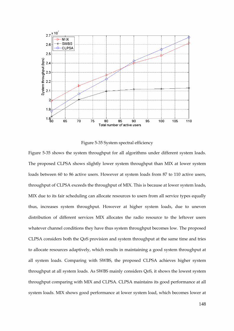
148
Figure 5-35 System spectral efficiency
Figure 5-35 shows the system throughput for all algorithms under different system loads.
The proposed CLPSA shows slightly lower system throughput than MIX at lower system
loads between 60 to 86 active users. However at system loads from 87 to 110 active users,
throughput of CLPSA exceeds the throughput of MIX. This is because at lower system loads,
MIX due to its fair scheduling can allocate resources to users from all service types equally
thus, increases system throughput. However at higher system loads, due to uneven
distribution of different services MIX allocates the radio resource to the leftover users
whatever channel conditions they have thus system throughput becomes low. The proposed
CLPSA considers both the QoS provision and system throughput at the same time and tries
to allocate resources adaptively, which results in maintaining a good system throughput at
all system loads. Comparing with SWBS, the proposed CLPSA achieves higher system
throughput at all system loads. As SWBS mainly considers QoS, it shows the lowest system
throughput comparing with MIX and CLPSA. CLPSA maintains its good performance at all
system loads. MIX shows good performance at lower system load, which becomes lower at

149
higher system loads. This is because MIX cannot adapt itself to uneven distribution of
services, which becomes more affective at higher system loads.
The proposed CLPSA is capable to maintain better performance in the changing network
scenarios as compared to the state-of-the-art QoS aware MIX and SWBS algorithms. This is
because CLPSA allocates resources to different services adaptively based on the achieved
QoS, changing network conditions and variable system load, by using information on QoS
measurements.
Performance Analysis of CLPSA 5.4.5
In the previous section, the performance of proposed CLPSA is compared with QoS aware
SWBS and MIX algorithms under changing network scenarios. The proposed CLPSA is
adaptive to the changing traffic patterns and variable number of active users. To validate it,
this section gives the self-comparison of the proposed CLPSA under different scenarios.
Figure 5-36 Average packet delay of real-time service

150
Figure 5-36 shows the average packet delay of real-time service for CLPSA under different
system loads for all scenarios. It is very low in scenarios I, 3 and 4 in which real-time service
is not dominant. However in scenario 2 where real-time service is dominant over all other
services, the average packet delay increases with system load showing a value of 14 ms at
the highest system load. However average packet delay remains under the delay upper
bound which is 40 ms in LTE-A networks.
Figure 5-37 Average packet drop rate of real-time service
Average PDR of real-time service under different system loads for all scenarios is shown in
Figure 5-37. In the First two scenarios, CLPSA shows the same trend of PDR and is
increasing with the system load. This is because RT users are more in number in these
scenarios as compared to the rest two scenarios. The total percentage of RT users is in these
scenarios is equivalent to 50 % and 70 % of total system load, respectively. However in
scenarios 3 and 4, average PDR is decreasing with system load because in these scenarios,
RT users are only 20% of the total system load. However under all network scenarios,
average PDR remains below the PDR threshold, which is 0.1 for LTE-A networks.

151
Figure 5-38 Standard deviation of average PDR distribution of RT users
Figure 5-38 shows STD of average PDR for all RT users with system loads, under different
network scenarios. It remains under the PDR threshold (o.1) at all system loads and under
all network scenarios. Scenario 2 however behaves differently by showing increasing STD
values with system load, which becomes constant above 100 active users. This is because in
scenario 4, real-time service is dominant over all other services. In scenario 1, 3 and 4, real-
time service is not dominant, therefore STD values decrease with system load.

152
Figure 5-39 Average achieved throughput of streaming traffic
The average achieved throughput of streaming video service with system loads under
different network scenarios is shown in Figure 5-39. The throughput requirement of
streaming service is fulfilled in all scenarios except in scenario 4, in which streaming service
is dominant over all other traffic types. The reason is the massive number of users
demanding streaming service in this scenario. Under such condition, it is normal that all
users cannot be guaranteed their throughput requirements.
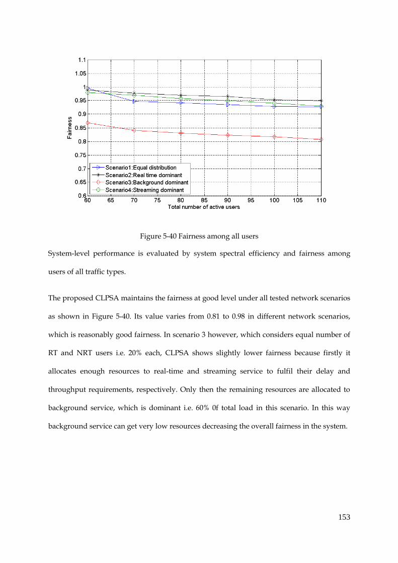
153
Figure 5-40 Fairness among all users
System-level performance is evaluated by system spectral efficiency and fairness among
users of all traffic types.
The proposed CLPSA maintains the fairness at good level under all tested network scenarios
as shown in Figure 5-40. Its value varies from 0.81 to 0.98 in different network scenarios,
which is reasonably good fairness. In scenario 3 however, which considers equal number of
RT and NRT users i.e. 20% each, CLPSA shows slightly lower fairness because firstly it
allocates enough resources to real-time and streaming service to fulfil their delay and
throughput requirements, respectively. Only then the remaining resources are allocated to
background service, which is dominant i.e. 60% 0f total load in this scenario. In this way
background service can get very low resources decreasing the overall fairness in the system.

154
Figure 5-41 System throughput
System throughput with system loads is shown in Figure 5-41, which varies from 15 Mbps to
27.8 Mbps under different scenarios. In scenario 3 the proposed scheduling architecture
shows lower system throughput as compared scenarios 1, 2 and 4. This is because the
proposed CLPSA first considers the QoS requirements of real-time voice and streaming
services. And users requiring these services may not have good channel condition, thus,
decrease overall system throughput in this scenario.
The results show that the proposed CLPSA maintains good scheduling performance both at
the user-level and at the system-level, under various network scenarios. It can work
appropriately when the load of different services including real-time, non-real time and
background is varied and also when the overall system load is varied from low to high.
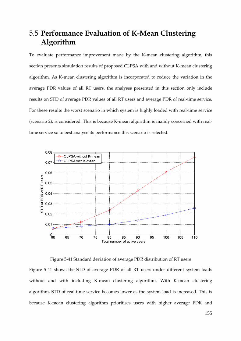
155
Performance Evaluation of K-Mean Clustering 5.5Algorithm
To evaluate performance improvement made by the K-mean clustering algorithm, this
section presents simulation results of proposed CLPSA with and without K-mean clustering
algorithm. As K-mean clustering algorithm is incorporated to reduce the variation in the
average PDR values of all RT users, the analyses presented in this section only include
results on STD of average PDR values of all RT users and average PDR of real-time service.
For these results the worst scenario in which system is highly loaded with real-time service
(scenario 2), is considered. This is because K-mean algorithm is mainly concerned with real-
time service so to best analyse its performance this scenario is selected.
Figure 5-41 Standard deviation of average PDR distribution of RT users
Figure 5-41 shows the STD of average PDR of all RT users under different system loads
without and with including K-mean clustering algorithm. With K-mean clustering
algorithm, STD of real-time service becomes lower as the system load is increased. This is
because K-mean clustering algorithm prioritises users with higher average PDR and

156
becomes more effective when number of users increase as grouping effect becomes
prominent. At lower system loads, due to smaller number of RT users, all users can get PRBs
and meet their QoS demands, thus, clustering has little effect. However at higher system
loads, when users are more in number, the competition to get PRBs becomes higher. In this
scenario K-mean clustering can further arrange the priority of RT users based on their
average PDR values and effectively lowers average PDR, which results in reduced STD of
RT users.
Figure 5-42 Average packet drop rate of real-time service
Figure 5-42 shows average PDR of real-time service under different system loads by using
CLPSA with and without K-mean clustering algorithm. Average PDR of real-time service
becomes lower at higher system loads when K-mean clustering algorithm is used. This is
because K-mean clustering has already effectively reduced average PDR of individual RT
users at highly loaded system, which ultimately reduces the average PDR of overall real-
time service.

157
Summary 5.6
In this chapter simulation results and their analyses on all novel algorithms, proposed in this
thesis, are presented. The performance of SSSA, Hebbian learning and K-mean Clustering
algorithm are presented and compared with two QoS aware state-of-the-art algorithms. The
overall performance of the packet scheduling architecture is tested under different network
scenarios to exemplify the real systems. The results show an improved QoS to real-time
service while fulfilling long-term rate requirements of non-real time service and maintaining
a good trade-off between user-level and system-level performance.

158
Chapter 6 Conclusions and Future Work
Conclusions 6.1
A cross layer packet scheduling architecture (CLPSA) is proposed in this thesis for the DL
transmission of LTE-A networks. In the CLPSA, two novel service specific queue sorting
algorithms (SSSA) are proposed for the real-time voice service and non-real time streaming
service, respectively, to improve user-level performance. An adaptive time domain
scheduling algorithm (ATDSA) is proposed, which integrates Hebbian learning process and
K-mean clustering algorithm to make scheduling decision by taking both system-level and
user-level performance into account. The performance of the proposed SSSA and ATDSA
including the effectiveness of K-mean clustering algorithm are investigated via system level
simulation. The overall performance of CLPSA is analysed under different network
scenarios including (i) equal distribution of real-time and non-real time services, (ii) real-
time service dominant, (iii) background service dominant and (iv) streaming service
dominant. The specific conclusions are:
The proposed SSSA for prioritising real-time service in the Traffic Differentiator can
effectively improve the QoS provision to RT users in terms of reduced average
packet delay and average PDR in comparison to QoS aware SWBS algorithm. This
performance improvement is more obvious at higher system load.
The K-mean clustering algorithm integrated in the TD Scheduler can further reduce
the average PDR of all RT users. In particular, it can effectively reduce the variation
in average PDR of individual RT users, which leads to better fairness among RT
users in terms of PDR. This phenomenon is most obvious in scenario (ii) where real-
time service is dominant.

159
The overall performance of the proposed CLPSA depends on the network scenarios:
o In all four scenarios, CLPSA outperforms SWBS and MIX in terms of average
packet delay of real-time service.
o In scenario (ii) where the real-time service is dominant, CLPSA reduces the
average packet delay and average PDR for real-time service in comparison
with SWBS and MIX. At system-level, CLPSA outperforms SWBS; it achieves
better fairness with a trade-off of a slight loss of system throughput as
compared to MIX.
o In scenario (iv) where the streaming service is dominant, CLPSA still achieves
lower average packet delay of real-time service compared to SWBS and MIX.
At system-level, compared to MIX, CLPSA shows similar performance;
compared to SWBS, CLPSA achieves better fairness and higher system
throughput with a trade-off of lower average throughput of steaming service.

160
Future Work 6.2
In this thesis, the main focus has been on scheduling in OFDMA-based LTE-A networks.
One aspect that has been established is that right techniques can significantly improve the
QoS provision to different services while maintaining a good trade-off between user-level
and system-level performance.
However, there are other techniques that can improve the user-level performance
particularly those near the cell edge. One such technique is relay-based OFDMA networks.
One of the approaches for further work could be applying the principles of the methods of
SSSA and ATDSA in relay-based networks. In particular, there has been no work focusing
on learning environment data and taking scheduling decision based on it, in relay-based
OFDMA networks so this is an area where there is significant potential.

161
References
[3GPP03} 3GPP Recommendation ITU-R M.1079-2, “Performance and quality of service
requirements for mobile telecommunications 2000 (IMT 2000) access
networks”, (1994-2000-2003).
[3GPP07] Recommendation ITU-R M.1822, “Framework for services supported by
IMT”, 2007.
[3GPP09a] 3GPP TSG-RAN TS 36.300, “Evolved universal terrestrial radio access (E-
UTRA) and evolved universal terrestrial radio access network (E-UTRANN)”,
version 9.0.0, June 2009.
[3GPP09b] 3GPP TSG-RAN TR25.814, “Physical layer aspects for evolved UTRA”,
version 7.0.0, June (2006-2009).
[3GPP09c] 3GPP Report ITU-R M.2135-1, “Guidelines for evolution of radio interface
technologies for IM-Advanced”, Dec. 2009.
[3GPP11a] 3GPP TS 36.101, “Evolved universal terrestrial radio access (E-UTRA); user
equipment (UE) radio transmission and reception”, version 10.4.0, Sep. 2011.
[3GPP11b] 3GPP Technical Specification group Radio Access Networks TR 36.913,
“Requirements for Evolved UTRA (E-UTRA) and Evolved UTRAN (E-
UTRAN)”, version 10.0.0 (2011-03).
[3GPP12a] 3GPP TR 36.912, “Feasibility study for further advancements for E-UTRA
(LTE-Advanced)”, Release 9, 2009-2012.
[3GPP12b] 3GPP TR 36.912, “Feasibility study for further advancements for E-UTRA
(LTE-Advanced)”, version 9.1.0 (2009-2012), pp. 42-43.
[3GPP12c] 3GPP TS 23.203, “Policy and charging control architecture”, Release 10, 2012.
[3GPPLTE12d] www.3gpp.org/Technologies/Keywoeds-Acronyms/LTE,
“The mobile broadband standards”, New opportunities for 3GPP in Rel-12,

162
Barcelona 12th Dec. 2012.
[Adachi02] F. Adachi, “Evolution towards broadband wireless systems”, proceedings of
the international symposium on wireless personal multimedia
communications (WPMC), Vol. 1, Honolulu, Hawaii, October 2002, pp. 19-26.
[AG11] M. F. L. Abdullah and M. F. Ghanim, “An overview of CDMA technologies
for mobile communications”, A journal of mobile communication, Vol.5, 2011,
pp. 16-24.
[AKRSW01] M. Andrews, K. Kumaran, K. Ramanan, A. Stolyar and P. Whiting, "Providing
Quality over a shared wireless link”, IEEE communications magazine, Vol. 39,
issue 2, February 2001, pp. 150-154.
[AM08] M. Assaad, A. Mourad, ”New frequency-time scheduling algorithms for
3GPP/LTE-like OFDMA air interface in the downlink”, IEEE vehicular
technology conference (VTC), 2008, pp. 1964-1969.
[APY95] J. B. Anderson, T. S. Rappaport and S. Yoshida, “Propagation measurements
for wireless communication channels”, IEEE communication magazine, Vol.
33, issue, 1 Jan. 1995, pp. 42-44.
[AWEweb12] www-awe-communications.com/Propagation/Urban/COST/index.htm,
“COST 231 Walfisch-Ikegami Model”, retrieved on Jan. 2012.
[Adas97] A. Adas, “Traffic models in broadband networks”, IEEE communication
magazine, Vol. 35, issue 7, July 1997, pp. 82-89.
[CJAV05] W. Christian, O. Jan, G. E. Alexander, E. Von, ”Fairness and throughput
analysis for generalized proportional fair scheduler in fourth generation
wireless systems”, IEEE vehicular technology conference VTC-spring. 2005,
pp. 1095-1098.
[CZWS10] J. Chen, L. Zhu, Q. Wu, Z. Shen, ”Multi-services supporting weighted power
scheduling algorithm based on LWDF”, IEEE international conference on
wireless communications and signal processing (WCSP) 2010, pp. 1-5.

163
[CD07] B. Chisung and Dong-Ho, “Fairness-aware adaptive resource allocation
scheme in multihop OFDMA systems”, IEEE communication letters, Vol. 11,
issue 2, Feb. 2007, pp. 134-136.
[Chandrasekaran06] B. Chandrasekaran, “Survey of network traffic models”, 2006, retrieved on
Sep.2010 from:
http://www.cse.wustl.edu/~jain/cse567-06/ftp/traffic_models3.pdf
[DPSB08] E. Dahlman, S. Parkvall, J. Skold and P. Bening, “3G Evolution; HSPA and
LTE mobile broadband”, 2nd Ed., ISBN 978-0-12-374538-5, pp. 31-34.
[EFKMPTW06] H. Ekstrom, H. Furuskar, J. Karlsson, M. Meyer, S. Parkvall, J. Trsner, and M.
Wahlqvist, ”Technical solution for 3G LTE”, IEEE communications magazine,
Vol. 44, issue 3, March 2006, pp. 38-45.
[EHSB01] V. Erceg, K. V. S. Hari, M. S. Smith and D. S. Baum, “Channel models for fixed
wireless applications”, contribution to IEEE 802.16.3, July 2001.
[FL96] B. H. Fleury and P. E. Leauthold, “Radiowave propagation in mobile
communications: an overview of European research”, IEEE communication
magazine, Vol. 34, issue 2, Feb. 1996, pp. 70-81.
[GBP08] I. Gutierrez, F. Bader, J. L. Pijoan, “Prioritization function for packet
scheduling in OFDMA systems”, proceedings of annual international
conference on wireless Nov. 2008, article no. 19.
[Goldsmith05] A. Goldsmith, “Wireless communications”, Cambridge University press 2005,
ISBN 978-0-521-83716-3, pp. 10-12.
[GS97] A. J. Goldsmith and C. Soon-Ghee, “Variable-power MQAM for fading
channels”, transaction on IEEE communications, Vol. 45, 1997, pp. 1218-1230.
[GPKM08] M. Guillaume, K. I. Pedersen, I. Z. Kovacs and P. E. Mogensen, “QoS oriented
time and frequency domain packet schedulers for the UTRAN Long Term
Evolution”, Proceedings of the IEEE vehicular technology conference (VTC),
Singapore, May 2008, pp. 2532-2536.
164
[Hashmi93] H. Hashmi, “The indoor propagation channel”, proceedings of the IEEE, Vol.
81, issue 7 July 1993, pp. 943-968.
[HT09] H. Harri, A. Toskala, “LTE for UMTS OFDMA and SC-FDMA based radio
access”, John Wiley & Sons, ISBN 978-0-470-99401-6 (H/B), 2009, pp. 5-6.
[Hebb49] D. O. Hebb (1949), “The organization of behaviour”, Wiley: New York, 1949.
[Haykin08] S. Haykin, “Neural networks and learning machines”, 3rd Ed., Vol. 10, ISBN-
10: 0131471392, 2008.
[JN87] A. J. I. Jinning, and P. L. S. Nicholson, “Artificial intelligence in
communication networks”, conference on computing systems and
information technology, 1987.
[Jayakumari10] J. Jayakumari, “MIMO-OFDM for 4G wireless systems”, international journal
of engineering science and technology, Vol. 2, issue 7, 2010.
[JL03] J. Jang and K. B. Lee, “Transmit power adaptation for multiuser OFDM
systems”, IEEE journal on selected areas in communication, Vol. 21, issue 2,
2003, pp. 171-178.
[JWY05] A. Jamalipour, T. Wada and T. Yamazato, “A tutorial on multiple access
technologies for beyond 3G mobile networks”, IEEE communications
magazine, Vol. 43, issue 2, Feb. 2005, pp. 110-117.
[KSA08] C. B. Kian, A. Simon, D. Angela, “Joint time-frequency domain proportional
fair scheduler with HARQ for 3GPP LTE Systems”, IEEE vehicular technology
conference 2008, VTC-Fall, pp. 1-5.
[Kumar09] S. Kumar, “Techniques of efficient spectrum usage for next generation mobile
communication networks-LTE and LTE-Advances study“, doctoral
dissertation, University of Aalborg Denmark, June 2009.
[KALNN05] H. Kaaranen, A. Ahtiainen, S. Naghian, and V. Neime, Eds, “UMTS networks,
165
architecture, mobility and services”, 2nd Ed. John Wiley & Sons, ISBN 978-0-
470-01103-4, 2005.
[KH10] F. Khozeimeh, S. Haykin, “Self-organizing dynamic spectrum management
for cognitive networks”, communication networks and services conference
(CNSR), 2010, pp. 1-7.
[LL05] H. Liu and G. Li, “OFDM-based broadband wireless networks design and
optimizations”, John Willay & Sons, ISBN 978-0-471-72346-2, 2005.
[Molkdar91] D. Molkdar, “Review on radio propagation into and within buildings”, IEEE
Proceedings on microwave, antennas and propagation, Feb 1991, Vol. 138,
issue 1, pp. 61-73.
[NH06] T. Nguyen, Y. Han,”A proportional fairness algorithm with QoS provision in
downlink OFDMA systems”, IEEE communication letters, Nov. 2006, Vol. 10,
issue 11, pp. 760-762.
[PBA05] P. Parag, S. Bhashyam, and R. Aravind, “A subcarrier allocation algorithm for
OFDMA using buffer and channel state information”, IEEE vehicular
technology conference, VTC-2005-Fall, 2005, pp. 622-625.
[PJNTTM03] K. Petter, P. Jani, K. Niko, R. Tapani, H. Tero, M. Martti, ”Dynamic packet
scheduling performance in UTRA Long Term Evaluation downlink”, IEEE
international symposium on wireless pervasive computing (ISWPC), 2008,
pp. 308-313.
[JNTMM08] P. Jani, K. Niko, H. Tero, M. Martti and R. Mika, “Mixed traffic packet
scheduling in UTRAN Long Term Evaluation downlink”, IEEE international
symposium on personal, indoor and mobile radio communications (PIMRC),
2008, pp. 1-5.
[Proakis01] J. G. Proakis, “Digital communications”, ISBN 0-07-232111-3, McGraw-Hill,
New York, 2001.

166
[PKVP06] S. Petridou, V. Koutsonikola, A. Vakali and G. Papadimitriou, “A divergence-
oriented approach for web-users clustering”, proceedings of ICCSA, 2006, pp.
1229-1238.
[PPMRKM07] A. Pokhariyal, K. I. Pedersen, G. Monghal, I. Z. Kovac, C. Rosa, T. E. Kolding
and P. E. Mogensen, ”HARQ aware frequency domain packet with different
degrees of fairness for UTRAN LTE”, IEEE vehicular technology conference
(VTC ) 2007, pp. 2761-2765.
[PR80] A. Peled, A. Ruiz, ”Frequency domain data transmission using reduced
computational complexity algorithms”, proceedings of ICASSP 1980, Vol. 5,
pp. 964-967.
[PSPP07] S. G. Petridou, P. G. Sarigiannidis, Georgios I. Papadimitriou, A. S.
Pomportsis, “Clustering based scheduling: A new approach to the design of
scheduling algorithms for WDM star networks”, IEEE symposium on
communications and vehicular technologies 2007, pp. 1-5.
[Rappaport02] T. S .Rappaport, “Wireless communications, principles and practice”, 2nd Ed.,
ISBN 0-13-042232-0, 2002, pp. 177-179.
[RM86] D. E. Rumelhart, J. L McClelland and PDP research group, “Parallel
distributed processing: Explorations in the microstructure of cognition”,
Cambridge Press, Vol. 1, ISBN 0-262-68053-X, 1986.
[RokeLTE13] Roke, “LTE MAC scheduler & radio bearer QoS”, retrieved on Jan. 2013 from,
www.roke.co.uk/resources/white-papers/0485-LTE-Bearer-QoS.pdf
[Senarath07] G. Senarath, “Multi-Hop relay system evaluation methodology: Channel
model and performance metric”, IEEE 802.16 broadband wireless access
working group, Feb. 2007.
[SLC06] D. Soldani, M. Li, and R. Cuny, “QoS and QoE management in UMTS cellular

167
networks”, John Willey & Sons Ltd, ISBN 978-0-470-01639-8, 2006.
[SR2000] A. L. Stolyar and K. Ramanan,” Largest weighted delay first scheduling:
Large deviations and optimality”, The annals of applied probability, Vol. 11,
No. 1, February 2000, pp. 1-48.
[Shannon48] C. E. Shannon, “A mathematical theory of communication”, Bell system
technical journal, Vol. 27, July and Oct. 1948, pp. 379-423.
[SYLX09] J. Shen, N. Yi, A. Liu and H. Xiang, “Opportunistic scheduling for
heterogeneous services in downlink OFDMA system”, IEEE international
conference on communications and mobile computing, computer Society
2009, pp. 260-264.
[SCDT00] J. Srivastava, R. Cooley, M. Deshpande and P. N. Tan, “Web usage mining:
discovery and application of usage patterns from web data”, SIGKDD
Explorations, Vol. 1, No. 2, 2000, pp. 12-23.
[TCT10] T. U. Tsai, Y. L. Chung and Z. Tsai, “Communications and networking”, ISBN
978-953-114-5, published on Sep. 2010 under CCBY-NC-SA 3.0 licence, pp.
264-288.
[TV05] D. Tse, and P. Viswanath, “Fundamentals of wireless communication”,
Cambridge University Press, 2005.
[WA93] W. Bechtel, and A. Abrahamsen, “Connectionism and the mind”, ISBN-10:
0631207120, Oxford, UK, Blackwell, 2002.
[WXZXY03] A. Wang , L. Xio, S. Zhou, X. Xu, Y. Yao, ”Dynamic resource management in
the fourth generation wireless systems”, proceedings of communication
technology, Vol. 2, ICCT international conference April 2003, pp. 1095-98.
[XC08] L. Xu, L. Cuthbert., “Improving fairness in relay-based access networks”,
proceedings of international symposium on modelling, analysis and

168
simulation of wireless and mobile systems (MSWIM) in ACM Nov. 2008, pp.
18-22.
[XCSCZ11] L. Xu, Y.Chen, J. Schormans, L. Cuthbert, T. Zhang, “User-vote assisted self-
organizing load balancing for OFDMA cellular systems”, IEEE international
symposium on personal, indoor and mobile radio communications (PIMRC)
2011, pp. 217-221.
[XW05] R. Xu and D. Wunsch,”Survey of Clustering Algorithms”, IEEE transaction
on neural networks, Vol.16, no.3, May 2005, pp. 645-78.
[Yang05] H. Yang, “A road to future broadband wireless access: MIMO-OFDM-based
air interface”, IEEE communication magazine, Vol. 43, no. 1, Jan. 2005, pp. 53-
60.
[ZP02] G. Zhang, advisor prof. Panwar, “EL938 Report: Packet scheduling”, April
2002.