qmc.psi - comp-phys.org
TRANSCRIPT

1ALPS Tutorial – PSI 08/09/2006
A Quick introduction to A Quick introduction to Quantum Monte Carlo Quantum Monte Carlo methodsmethods
Fabien Alet LPT, Univ. Paul Sabatier Toulouse
Contact : [email protected]
2F. Alet (Toulouse) – Introduction to QMC – ALPS Tutorial PSI
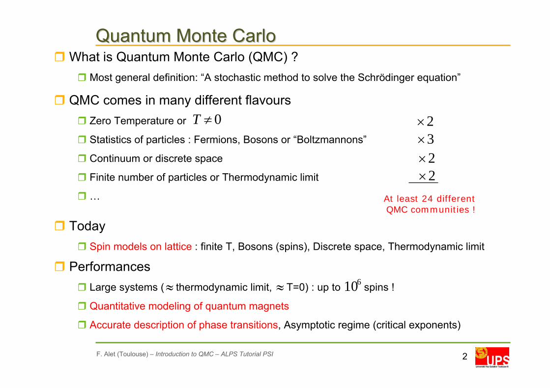
Quantum Monte CarloQuantum Monte CarloWhat is Quantum Monte Carlo (QMC) ?
Most general definition: “A stochastic method to solve the Schrödinger equation”
QMC comes in many different flavoursZero Temperature or
Statistics of particles : Fermions, Bosons or “Boltzmannons”
Continuum or discrete space
Finite number of particles or Thermodynamic limit
…
0≠T 2×
2×2×
3×
TodaySpin models on lattice : finite T, Bosons (spins), Discrete space, Thermodynamic limit
At least 24 different QMC communities !
PerformancesLarge systems ( thermodynamic limit, T=0) : up to spins !
Quantitative modeling of quantum magnets
Accurate description of phase transitions, Asymptotic regime (critical exponents)
≈ ≈ 610

3F. Alet (Toulouse) – Introduction to QMC – ALPS Tutorial PSI
QMC = a large family tree QMC = a large family tree « Variational Monte Carlo » family
« Diffusion Monte Carlo » familyProjector Monte Carlo, Green Function Monte Carlo, Diffusion Monte Carlo (+ Fixed Node, +
Stochastic Reconfiguration) …
(Partial) Ref. for lattice models : S. Sorella and L. Capriotti, Phys. Rev. B 61, 2599 (2000)
« Determinental Monte Carlo » familyAuxiliary Field Monte Carlo, Determinental Monte Carlo, Hirsch-Fye …
(Partial) Ref. for lattice models : F. F. Assaad, Lecture Notes, NIC series 10, 99 (2003)
« Path integral Monte Carlo » familyLattice systems (cluster algorithms)
Basic Idea : Mapping Quantum system in dimension d → Classical system in dimension d+1
Then do classical Monte Carlo on the equivalent problem

4ALPS Tutorial – PSI 08/09/2006
A Quick introduction to A Quick introduction to Quantum Monte Carlo Quantum Monte Carlo methodsmethodsfor for latticelattice quantum spin quantum spin modelsmodels
Derivation of configuration space : Path integral approach
Monte Carlo moves : quantum cluster algorithms
The sign problem
Practical considerations

5F. Alet (Toulouse) – Introduction to QMC – ALPS Tutorial PSI
Quantum Monte Carlo simulationsQuantum Monte Carlo simulationsNot as « easy » as classical Monte Carlo
Calculating the energy eigenvalue Ec = solving the problem
Need to find a mapping of the quantum partition function to a
classical problem
Different approachesPath integrals (time-dependent perturbation theory in imaginary time)
Stochastic Series Expansion (high temperature expansion)
Sign problem if some pc < 0 (thus try to avoid this)
Then need efficient updates for the equivalent classical problem
∑ −− ==c
EH ceeZ ββTr
∑≡= −
cc
H peZ βTr

6F. Alet (Toulouse) – Introduction to QMC – ALPS Tutorial PSI
Hamiltonian of spin ½ modelsHamiltonian of spin ½ modelsExample : XXZ model in a field
Anisotropic exchange interactions : JXY , JZ
Magnetic field h
Heisenberg model : JXY = JZ = J
Hamiltonian matrix in 2-site basis
∑∑
∑∑
−++=
−++=
+−−+
i
zi
ji
zj
zizjiji
XY
i
zi
ji
zj
ziz
yj
yi
xj
xiXYXXZ
ShSSJSSSSJ
ShSSJSSSSJH
,
,
)(2
)(
∑∑ −=i
zi
jiji ShSSJH
,
rr
{ } , , , ↓↓↓↑↑↓↑↑⎟⎟⎟⎟⎟⎟⎟⎟⎟
⎠
⎞
⎜⎜⎜⎜⎜⎜⎜⎜⎜
⎝
⎛
−
−
−
+
=
hJ
JJ
JJ
hJ
H
z
zxy
xyz
z
ij
4000
042
0
024
0
0004

7F. Alet (Toulouse) – Introduction to QMC – ALPS Tutorial PSI
Trotter decompositionTrotter decompositionBasis of most QMC algorithms
Here : Generic mapping of a quantum spin system onto a classical Ising model
Not limited to special cases
Split Hamiltonian into two easily diagonalizable pieces
Obtain a decomposition of the partition function
Insert 2M sets of complete basis states
=
+
H
H1
H2
])Tr[( Tr Tr )()( 2121 MHHHHH eeeZ +Δ−+−− === τββ
)(])Tr[( 221 τττ Δ+= Δ−Δ− Oee MHH
ieiieiieiieiMii
HHM
HMM
H∑ Δ−Δ−−
Δ−Δ− ⋅⋅⋅=21
2121
,...,122312221
ττττ
)/( Mβτ =Δ
H(1) H(2) H(3) H(4)
21 HHH +=
)( 221 εεεε Oeee HHH += −−−

8F. Alet (Toulouse) – Introduction to QMC – ALPS Tutorial PSI
Example : Spin ½ Heisenberg modelExample : Spin ½ Heisenberg model
Quantum problem in d dimensions maps onto a classical problem in d+1Expand the states in the Sz eigenbasis
Effective Ising-model in d+1 dimensions with 2- and 4-sites interaction terms
Each of the matrix
elements
corresponds to a row of
shaded plaquettes and
equals the product over
those plaquettes
αi
21
2121
,...,122312221 ieiieiieiieiZ
Mii
HHM
HMM
H∑ Δ−Δ−−
Δ−Δ− ⋅⋅⋅= ττττ
jH
j iei 2,11
τΔ−+
Conservation of
magnetization :
Continuous worldlines

9F. Alet (Toulouse) – Introduction to QMC – ALPS Tutorial PSI
Weights for the spin ½ Heisenberg modelWeights for the spin ½ Heisenberg modelThe partition function becomes a sum of products of plaquette weights
The only allowed plaquette-configurations are (here h=0)
Ferromagnet (J<0) : All weights are positive
Antiferromagnet on a bipartite lattice : perform a gauge transformation on one sublattice
Frustrated antiferromagnet : we have a sign problem
)( )(
∑ ∏∑ ==C pplaquettes
pC
CwCWZ
( ) ( )+−−+±±
+−−+ +−⎯⎯⎯⎯⎯⎯ →⎯ −→+ jijii
ii
jiji SSSSJSSSSSSJ
2 )1(
2
)2/(4/ Jche J ττ ΔΔ )2/(4/ Jshe J ττ Δ−Δ4/Je τΔ−

10F. Alet (Toulouse) – Introduction to QMC – ALPS Tutorial PSI
)( )(
∏=pplaquettes
pCwCW
)2/(4/ Jche J ττ ΔΔ )2/(4/ Jshe J ττ Δ−Δ4/Je τΔ−
WorldlineWorldline approach : Summaryapproach : SummaryEach valid configuration = continuous worldlines on checkerboard
Worldline QMC = Sampling over all (important) worldline configurationsAccording to the above weight
Try to generate a new configuration from a given one
Already 2 problems arise …

11F. Alet (Toulouse) – Introduction to QMC – ALPS Tutorial PSI
Intermezzo 1 : Stochastic Series Expansion (SSE)Intermezzo 1 : Stochastic Series Expansion (SSE)
Alternative approach : Expansion in inverse temperature
Using the bond Hamiltonians
Similar to path integral approach
(Minor) difference in the treatment of diagonal terms
( )ααβ
β
α
β
∏∑ ∑∑
∑
=
∞
=
∞
=
−
−=
−==
n
ib
bbn
n
n
n
nH
i
n
Hn
Hn
eZ
1,...,0
0
)( !
)Tr(!
)Tr(
1
∑=
=),( jib
bHH
Hd(1,2)
i
54321
configuration operator
Ho(3,4)
Hd(3,4)
Ho(3,4)
1 2 3 4
Hd(1,2)
( )zj
zi
zj
ziz
dji
jijixyo
ji
SSzhSSJH
SSSSJ
H
+−=
+= +−−+
),(
),( )(2
(Sandvik, 1992)

12F. Alet (Toulouse) – Introduction to QMC – ALPS Tutorial PSI
1st solved problem : the continuous time limit1st solved problem : the continuous time limit
Systematic error due to finite value of Δτ (« Trotter error »)Need to perform an extrapolation to Δτ → 0 from simulations with different
values of Δτ (or Trotter number M)
The limit Δτ → 0 can be taken directly in the construction of the algorithm !
(Prokof’ev et al., 1996)
Number of changes
stays finite as
Different computational approach:Discrete time : store configuration at all time steps
Continuous time : store times at which configuration changes (+ initial state)
22JJMNc
βτ→
Δ=
0→Δτ
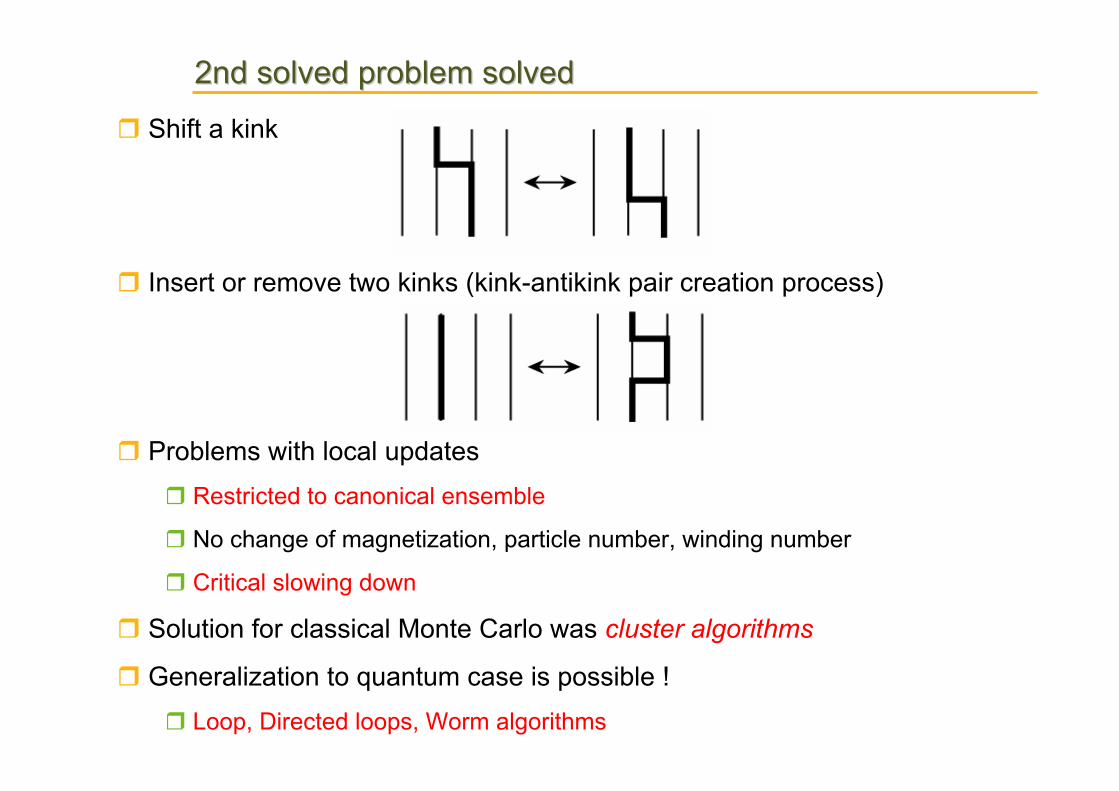
2nd solved problem solved2nd solved problem solved
Shift a kink
Insert or remove two kinks (kink-antikink pair creation process)
Problems with local updatesRestricted to canonical ensemble
No change of magnetization, particle number, winding number
Critical slowing down
Solution for classical Monte Carlo was cluster algorithms
Generalization to quantum case is possible !Loop, Directed loops, Worm algorithms

14F. Alet (Toulouse) – Introduction to QMC – ALPS Tutorial PSI
Worm algorithm : intuitive viewWorm algorithm : intuitive view
Q : How to update non-locally this configuration ?
(SSE Representation)1 2 3 4 5
15F. Alet (Toulouse) – Introduction to QMC – ALPS Tutorial PSI
1 2 3 4 5
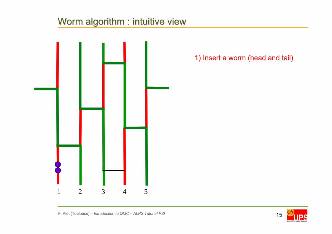
Worm algorithm : intuitive viewWorm algorithm : intuitive view
1) Insert a worm (head and tail)

16F. Alet (Toulouse) – Introduction to QMC – ALPS Tutorial PSI
1 2 3 4 5
Worm algorithm : intuitive viewWorm algorithm : intuitive view
1) Insert a worm (head and tail)
2) Move the worm head – Modify locally the configuration on the fly

17F. Alet (Toulouse) – Introduction to QMC – ALPS Tutorial PSI
Worm algorithm : intuitive viewWorm algorithm : intuitive view
“jump” “turn” “bounce”
3) At every “vertex” : Choose an exit
1) Insert a worm (head and tail)
2) Move the worm head – Modify locally the configuration on the fly
1 2 3 4 5 “straight”

18F. Alet (Toulouse) – Introduction to QMC – ALPS Tutorial PSI
Worm algorithm : intuitive viewWorm algorithm : intuitive view
1 2 3 4 5
1) Insert a worm (head and tail)
2) Move the worm head – Modify locally the configuration on the fly
“straight”, “jump”, “turn”, “bounce”3) At every “vertex” : Choose an exit

19F. Alet (Toulouse) – Introduction to QMC – ALPS Tutorial PSI
Worm algorithm : intuitive viewWorm algorithm : intuitive view
1) Insert a worm (head and tail)
2) Move the worm head – Modify locally the configuration on the fly
1 2 3 4 5
“straight”, “jump”, “turn”, “bounce”3) At every “vertex” : Choose an exit

20F. Alet (Toulouse) – Introduction to QMC – ALPS Tutorial PSI
Worm algorithm : intuitive viewWorm algorithm : intuitive view
1) Insert a worm (head and tail)
2) Move the worm head – Modify locally the configuration on the fly
1 2 3 4 5
“straight”, “jump”, “turn”, “bounce”3) At every “vertex” : Choose an exit
4) Annihilate worms

21F. Alet (Toulouse) – Introduction to QMC – ALPS Tutorial PSI
Worm algorithm : intuitive viewWorm algorithm : intuitive view
1) Insert a worm (head and tail)
2) Move the worm head – Modify locally the configuration on the fly
1 2 3 4 5
“straight”, “jump”, “turn”, “bounce”3) At every “vertex” : Choose an exit
4) Annihilate worms
NEW CONFIGURATION

22F. Alet (Toulouse) – Introduction to QMC – ALPS Tutorial PSI
Intermezzo 2 : How to choose the worm’s moves ?Intermezzo 2 : How to choose the worm’s moves ?
Given a “vertex” (plaquette) configuration and an entrance leg, where to exit ?
Consider exit leg e, given entrance leg i at a vertex in configuration c – weight w(c)
Assign this path a probability
Sum over all paths must equal unity
Choose exit leg e with probability leading to configuration c – weight w(c)
Consider the reverted path , leading back to c
Impose Local detailed balance
),|( cieP∑ =
e
cieP 1),|(
zhJcw Z +−=
2)(
),1|1( cP ),1|2( cP ),1|3( cP ),1|4( cP
),|( cieP
),|( ceiP
)(),|()(),|( cwceiPcwcieP =

Quantum cluster algorithmsQuantum cluster algorithms
Tiny differences in how the worm exactly moves lead to different algorithmsWorm algorithm : random Metropolis move
Directed loop algorithm : locally improved « clever » move
Loop algorithm : deterministic move
Difference in RepresentationSSE : usually slighlty faster
Path Integral (PI) : good when large diagonal terms
Codes in ALPS : Which qlgorithm to choose ?looper = Loop algorithm in PI/SSE : For models with spin inversion symmetry
e.g. : Heisenberg, XY, XXZ model wihout field
dirloop-sse = Directed loops in SSE : Models without inversion symmetry (most genera
e.g. : models with field, boson models etc
worm = Worm algorithm in PI : Models with large diagonal elements
e.g. : large Ising anisotropy
All these algorithms give accurate results for large systems …

24F. Alet (Toulouse) – Introduction to QMC – ALPS Tutorial PSI
Intermezzo 3 : The sign problemIntermezzo 3 : The sign problem
In mapping of quantum to classical system
« Sign problem » if some of the pi<0Cannot interpret pi as probabilities
Appears in simulation of fermions and frustrated magnets
“Way out” : Perform simulations using |pi| and measure the sign :
Sampling
[ ][ ] ∑
∑=
−−
=
i
i
)exp(Tr)exp(Tr
i
ii
p
pA
HHAA
ββ
p
p
iii
iiii
i
ii
Sign
SignA
ppp
pppA
p
pAA
sgn
sgn
ii
ii
i
i ≡==∑∑∑∑
∑∑
∑=i
ip pZ ||
25F. Alet (Toulouse) – Introduction to QMC – ALPS Tutorial PSI
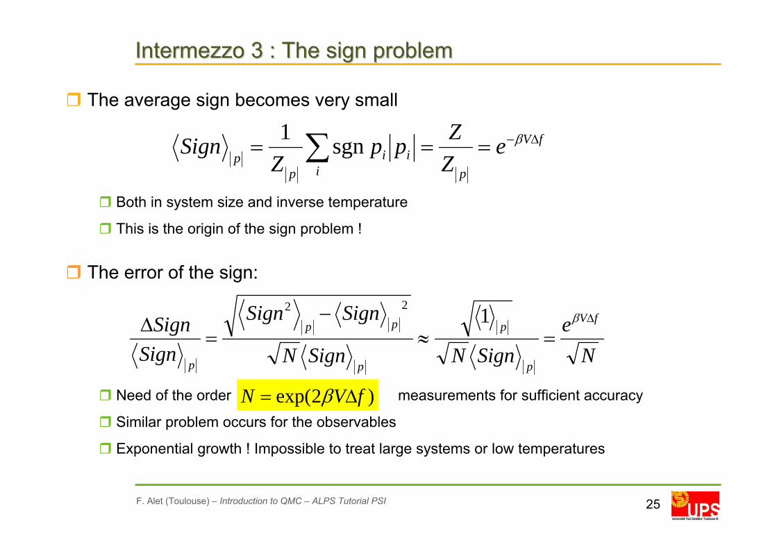
Intermezzo 3 : The sign problemIntermezzo 3 : The sign problem
The average sign becomes very small
Both in system size and inverse temperature
This is the origin of the sign problem !
The error of the sign:
Need of the order measurements for sufficient accuracy
Similar problem occurs for the observables
Exponential growth ! Impossible to treat large systems or low temperatures
fV
pi
ii
pp
eZZpp
ZSign Δ−=== ∑ βsgn1
Ne
SignNSignN
SignSign
SignSign fV
p
p
p
pp
p
Δ
=≈−
=Δ β122
)2exp( fVN Δ= β

26F. Alet (Toulouse) – Introduction to QMC – ALPS Tutorial PSI
In practice, what can I do ?In practice, what can I do ?
Simulate large samples of lattice quantum spin modelsFor non-frustrated models (Note : Diagonal (Ising) frustration is OK)
This includes most Heisenberg-like models
XY, Ising anisotropy, magnetic field, all values of S, single-ion anisotropy, …
Frustrated models are possible : but quickly sign problem arises
In all dimensions on all lattices (one can define its own specific lattice)
For all values of T (including T→0)
Which quantities are accessible ?A lot of observables : Energy, Specific heat, Susceptibilities, Structure factor,
Spin stiffness, Green functions …
In some cases : one can define its own observable
How much time ?Typically simulation time scales as Number of spins x Inverse Temperature
For more details : see hands-on session …

27ALPS Tutorial – PSI 08/09/2006
ThanksThanks !!