QIRANA: a Framework for Scalable Query Pricing

Shaleen DeepUniversity of Wisconsin-Madison

Madison, USAshaleen@cs.wisc.edu

Paraschos KoutrisUniversity of Wisconsin-Madison

Madison, USAparis@cs.wisc.edu

ABSTRACTUsers are increasingly engaging in buying and selling dataover the web. Facilitated by the proliferation of online mar-ketplaces that bring such users together, data brokers needto serve requests where they provide results for user queriesover the underlying datasets, and price them fairly accordingto the information disclosed by the query. In this work, wepresent a novel pricing system, calledQirana, that performsquery-based data pricing for a large class of SQL queries (in-cluding aggregation) in real time. Qirana provides priceswith formal guarantees: for example, it avoids prices thatcreate arbitrage opportunities. Our framework also allowsflexible pricing, by allowing the data seller to choose from avariety of pricing functions, as well as specify relation andattribute-level parameters that control the price of queriesand assign different value to different portions of the data.We test Qirana on a variety of real-world datasets andquery workloads, and we show that it can efficiently computethe prices for queries over large-scale data.

Categories and Subject DescriptorsH.2.4 [Systems]: Relational Databases

KeywordsData Pricing; Arbitrage; Query Determinacy

1. INTRODUCTIONThe last decade has seen an explosion of data being col-

lected from a variety of sources and across a broad rangeof areas. Many companies, including Bloomberg [7], Twit-ter [29], Lattice Data [19], DataFinder [11], and Banjo [4]collect such data, which then sell as structured (relational)datasets. Today, these datasets are often sold through onlinedata markets, which are web platforms for buying and sellingdata: examples include Microsoft Azure Marketplace [32],BDEX [5], and QLik DataMarket [24]. But such datasets areoften prohibitively expensive, since the sellers put a lot of

Permission to make digital or hard copies of all or part of this work for personal orclassroom use is granted without fee provided that copies are not made or distributedfor profit or commercial advantage and that copies bear this notice and the full citationon the first page. Copyrights for components of this work owned by others than theauthor(s) must be honored. Abstracting with credit is permitted. To copy otherwise, orrepublish, to post on servers or to redistribute to lists, requires prior specific permissionand/or a fee. Request permissions from permissions@acm.org.

SIGMOD’17, May 14 - 19, 2017, Chicago, IL, USAc⃝ 2017 Copyright held by the owner/author(s). Publication rights licensed to ACM.

ISBN 978-1-4503-4197-4/17/05. . . $15.00

DOI: http://dx.doi.org/10.1145/3035918.3064017

effort into obtaining, extracting, integrating, cleaning, andtransforming the data into a relational format. Existing datamarkets and data sellers either force users to buy the wholedataset, or support very simplistic pricing mechanisms (e.g.,they price according to output size). This means that valu-able data is often not accessible to lay users, scientists, orentities with limited budgets. In order to facilitate access todata for more users and expand the market for data-sellingcompanies and marketplaces, we need to tailor the purchaseof data to the user’s needs, by charging the user according tothe query workload rather than the full dataset: this is calledquery-based pricing. In this paper, we develop and evaluatean end-to-end framework for query-based pricing, and studyin detail the tradeoffs and design choices for building a com-prehensive query-based pricing system.

Previous work in this area studied the problem of pricingqueries both from a theoretical [16, 20, 21] and practical [18,30] point of view. This work identified a key principle in de-signing a pricing function, which is that it must not exhibitarbitrage: it should not be possible for a buyer to acquire thedesired query for a cheaper price by combining other queryresults. Pricing functions that exhibit arbitrage will lead toinconsistent pricing for queries, and can cause informationleakage. The pricing framework from [16, 18] works by re-quiring that the seller sets fine-grained price points (pricesto simple selection queries with equality predicates) that willbe used as a guide to price the other queries. In this set-ting, pricing join queries is in general NP-hard [16], but fora subclass of join queries it can be done in polynomial time.The QueryMarket prototype [18] showed that by formulat-ing the pricing problem as an ILP and using off-the-shelfILP solvers, one can price also the hard join queries, albeitfor small datasets. More recent work [30] considers simplis-tic pricing schemes, which assign a price according to thenumber of tuples that contribute to the answer, and provideno guarantees against arbitrage.

The above solutions proposed for a pricing framework allhave limitations. QueryMarket cannot handle queries withaggregation or grouping. Even for simple join queries, pric-ing is not scalable to even medium-sized datasets: for in-stance, [18] reports that computing a join query over a re-lation of about 1,000 tuples takes about one minute. Otherpricing schemes that assign a price to a query according toits output size, such as [30], are prone to arbitrage attacks.Thus, to the best of our knowledge, there is no existingquery-based pricing framework that prices a wide spectrumof SQL queries in real time, while providing formal guaran-tees about the properties of the pricing function.

We next provide a motivating example.

Example 1.1. Consider the Twitter database contain-ing two relations User and Tweet in Figure 1. Assume thatthe data seller fixes a price of $100 for the whole dataset andwants to price each individual relation at $50. Consider adata analyst, Alice, who wants to perform statistical analy-sis on demographics of twitter users. Alice cannot afford topurchase the whole dataset, but instead she would like to payaccording to the information content of a sequence of ana-lytics queries that she will ask over time. To begin with, sheasks about the number of female users on Twitter, by posingthe query Q1 = SELECT count(*) FROM User WHERE gen-

der = ’f’. Alternatively, she could ask the query Q2 =SELECT gender, count(*) FROM User GROUP BY gender toobtain the number of male and female users. If Q1 costs $7and Q2 costs $5, Alice has an arbitrage opportunity, becauseshe can get the same data (plus additional information) fromthe cheaper query Q2. The broker can avoid this arbitrageby pricing p(Q2) ≥ p(Q1), for example at $8.

Alice decides to buy Q2. Next, Alice wants to find out theaverage age of all Twitter users. She can ask for the queryQ3 = SELECT AVG(age) FROM User, which costs $11. How-ever, a different way to find the average age is to ask for thesum of age of all users and combine it with number of usersknown from Q2. Let Q4 = SELECT SUM(age) FROM User

and say that broker charges $2 for this query. Notice thatQ3 is more expensive than asking for both Q2 and Q4. Weagain have an arbitrage situation: to avoid this case, thebroker needs to make sure that p(Q3) ≤ p(Q2) + p(Q4).

Alice decides to purchase Q3 as well. Next, she asks Q5 =SELECT COUNT(*) FROM User WHERE gender=’m’, which hasoverlapping content with Q2. If the broker does not keeptrack of the purchase history, Alice will pay for the same in-formation twice and may go over her budget. Therefore, thebroker needs to take into consideration Alice’s query pur-chase history when pricing. In such a history-aware sce-nario, Q5 should be free.

Our Contribution. In this work, we describe, implementand evaluate a system for query-based pricing, called Qi-rana, that formally guarantees certain desirable properties.Our system works as an intermediate layer (broker) betweenthe DBMS and the data buyer. Once a buyer issues a queryQ on the database D, our pricing framework computes theoutput Q(D), and charges the user with a price p(Q,D).Qirana has the following characteristics:

• It allows the data seller to choose from several pricingfunctions, all of which provably avoid any arbitrageopportunities (Section 2.3).

• It supports efficiently history-aware pricing, where eachbuyer is charged not only according to the currentquery, but also according to past queries. This fea-ture prevents the buyer from overpaying when she hasalready acquired all or part of the desired information.

• It requires the seller to specify only a single price forthe whole dataset, without the need to provide mul-tiple fixed price points. In this case, our frameworktreats each part of the dataset as being equally valu-able. It also provides mechanisms so that the seller cantune the prices by specifying explicitly which relationsor attributes should be priced differently (Section 3.3).

• It provides an efficient and scalable implementation fora particular pricing function, called weighted coverage,

Useruid name gender age1 John m 252 Alice f 133 Bob m 454 Anna f 19

Tweettid uid time location1 3 23:29 CA2 3 23:29 WA3 1 23:30 OR4 2 23:31 CA

Figure 1: The database for the running example.

over a large class of SQL queries. In Section 5, we showthat Qirana can compute the price of queries overthe TPC-H and SSB datasets of scale factor 1 with a lowoverhead. Qirana is, to the best of our knowledge, thefirst query-based pricing system that allows real-timepricing with formal guarantees.

• It can be deployed on top of any DBMS without anymodification of the underlying database system.

Technical Overview. The key idea behind our pricingframework is as follows. From the point of view of thebuyer (Alice), there initially exists a set of possible databasesI, which captures the common knowledge about the data(schema, primary keys, data domain, etc.). Whenever Al-ice issues a query Q over the database D , she learns moreinformation, and can safely remove from I any database Dsuch that Q(D) = Q(D), thereby shrinking the number ofpossible databases. The price assigned to Q can then be for-mulated as a function of how much I shrinks. It turns outthat there are several choices of such a function that lead toarbitrage-free pricing functions [13].

Unfortunately, it is infeasible to keep track of all pos-sible databases, since their number can be astronomicallylarge. Our main observation is that instead of consideringall databases in I, it suffices to look only at a small subsetof I (which we call the support set): if we choose it carefully,it can approximate very well the amount of information dis-closed by returningQ(D). In particular, Qirana keeps trackof a subset S of neighboring databases of D in I: these arethe databases that differ from D only in one or two rows.For each neighboring database D ∈ S, our framework needsto compute Q(D), and check whether it agrees with Q(D).

This approach can compute the price for any query, butit requires that we compute Q over |S| databases, whichwe have to keep in the database along with D . Since thisis computationally and memory-wise expensive, we modeleach D ∈ S as an update applied to D (we can do thisbecause D , D are neighbors). To further speed up the exe-cution of the query Q on the updated database, we propose(Section 4) optimizations that allow us to check whether agiven update changes the output of the query, without need-ing to run the query again and again on the full database.Our proposed method can be of independent interest, sinceit can be applied to any view maintenance setting.

2. THE PRICING FRAMEWORKIn this section, we formally define the pricing framework

and introduce the notation used throughout the paper.

2.1 The Basics of PricingA data seller (Bob) wants to sell a database instance D

through a data market, which functions as the broker. Forinstance, suppose that Bob offers for sale the database in-stance in Figure 1. A data buyer (Alice) can purchase infor-mation from the dataset by issuing queries in the form of aquery bundle Q = (Q1, . . . , Qn), which is a vector of queries.

The queries can be formed in any query language, but forthis work we will focus on SQL queries. We denote the out-put of the query bundle by Q(D) = (Q1(D), . . . Qn(D)).

The database has a fixed schema R = (R1, . . . , Rk), whichis known to Alice. In addition to the schema, Alice possiblyhas more (public) knowledge about the database, such asfunctional or other types of dependencies (e.g. primary keys,foreign keys), domain constraints, or bounds on the size ofthe relations. For example, Alice knows that User.uid is aprimary key for User, Tweet.tid a primary key for Tweet, andthat there exists a foreign key dependency from Tweet.uidto User.uid. Let I denote the set of all possible databasesthat conform to the above constraints.

A pricing function p(Q, D) takes as input a query bundleQ and a database instance D ∈ I and assigns to it a price,which is a number in R+. Ideally, the price assigned shouldbe representative of the information that Alice learns fromobtaining the result Q(D). Depending on how the price iscomputed, there exists different types of pricing schemes.We adopt the terminology as introduced in [21]:

• Instance-independent (qps): The price depends onlyon Q, so p(Q, D) = p(Q, D′) for any D,D′ ∈ I.• Answer-dependent (aps): The price depends on Q

and the output E = Q(D). In other words, p(Q, D) =p(Q, D′) for any D,D′ ∈ I such that Q(D) = Q(D′).

• Data-dependent (dps): The price depends on bothQ and the database D.

We also say that Q1 determines Q2, denoted Q1 ↠ Q2,if whenever Q1(D) = Q1(D

′) then Q2(D) = Q2(D′) for

all D,D′ ∈ I.1 If Q1 determines Q2, then we can alwayscompute Q2 from the output Q1(D) without access to theunderlying database D. For example, coming back to Ex-ample 1.1, query Q2 determines query Q1. Similarly, we saythat Q1 determines Q2 under D, denoted D ⊢ Q1 ↠ Q2,if whenever Q1(D) = Q1(D

′) then Q2(D) = Q2(D′) for all

D′ ∈ I. Q1 ↠ Q2 implies that for every database D wehave D ⊢ Q1 ↠ Q2 but not the other way around.

2.2 Pricing DesiderataWhen we design a pricing function, there exist several de-

sirable properties we would like to guarantee, as well as takeinto account certain practical considerations. We next dis-cuss the various desiderata for a pricing function, both froma buyer’s and seller’s perspective. These desiderata form arich design space, with different trade-offs:

Information Arbitrage-Free Pricing We say that a pric-ing function is weakly information arbitrage-free if wheneverQ1 ↠ Q2 we have p(Q2, D) ≤ p(Q1, D) for every D. Wesimilarly say that it is strongly information arbitrage-free ifwhenever D ⊢ Q1 ↠ Q2 we have p(Q2, D) ≤ p(Q1, D). Tosee why the seller may require that a pricing function hasno information arbitrage, consider the example where theprice of a bundle Q1 is more than the price of bundle Q2

and Q1 reveals a subset of information than Q2. Then, Al-ice can choose to purchase Q2 and get the information ofQ1 for a price lower than intended. The strong informa-tion arbitrage condition is generally more desirable than theweak, since it is possible that Q1 ↠ Q2, but D ⊢ Q1 ↠ Q2

1We should note that this definition of determinacy isslightly different from the standard definition, where D,D′

can be any database instances (not necessarily from I).

for the particular database that is for sale. In this case, ifp(Q1,D) < p(Q2,D), the buyer will have an arbitrage op-portunity. Of course, since the underlying database D isunknown to the buyer, this opportunity will occur only bychance and not by following a particular strategy.

The requirement of strong information arbitrage-freenessconstraints our choice for a pricing function: any non-constantpricing function that is strongly information arbitrage-freemust also be aps ([13], Theorem 3.8), i.e. its price must de-pend on both Q and the output Q(D). Pricing schemes thatassign a price depending on the output size, or the prove-nance of the answer [30] offer no protection against arbi-trage. As a simple example, consider the query Q = SELECT

count(*) FROM R. A provenance-based approach would as-sign a full price to query Q since all tuples contribute to theoutput. Even if the provenance is extended to an attributelevel, there exist cases where boolean queries that check ifdatabase is empty cost substantially (see [21]).

Bundle Arbitrage-Free Pricing Consider the case whereAlice wants to obtain the answer for the bundleQ = Q1∥Q2,where ∥ denotes vector concatenation. Instead of asking forQ all at once, Alice can create two separate accounts, use oneto ask forQ1 and the other to ask forQ2. To avoid this issue,the seller must ensure that p(Q, D) ≤ p(Q1, D) + p(Q2, D)for all D ∈ I. In this case, we say that the pricing function isbundle arbitrage-free. Ensuring a bundle arbitrage-free pric-ing aps function can lead to disproportionately high pricesfor some queries, as shown in [13]. In particular, an apspricing function that exhibits no bundle arbitrage will priceany query, even one that touches a small part of the data, toat least half the full price of the dataset for many databaseinstances. On the other hand, presence of bundle arbitrageleads to arbitrage opportunities. This gives an importantdesign trade-off that a data seller needs to consider.

History-Aware Pricing In the context of a data market,Alice may want to issue multiple queries Q1, . . . , Qk overtime, some which may contain repeated information. Insuch a scenario, the data seller has two choices: (a) priceeach query individually, or (b) compute the price consider-ing the purchase history of queries for that particular buyer.If the seller chooses to price queries individually, then Al-ice will have to pay the amount

∑ki=1 p(Qi,D), in which

she could be charged multiple times for the same informa-tion. On the other hand, if the seller opts for history-awarepricing, then after issuing the first k queries, Alice will becharged with the amount p((Q1∥Q2 . . . ∥Qk),D); in otherwords, the whole sequence of the queries will be priced asa bundle. History-aware pricing can be implemented usingdifferent techniques, for example by issuing refunds [30], orby careful bookkeeping of what the buyer has already pur-chased.

Customizability The data seller should ideally be able tocustomize the pricing function as much or as less as possible.A customizable pricing function should be able to producevaried prices when the seller offers a single price point (theprice of the whole dataset), and also be able to incorpo-rate price suggestions from the seller. For example, Bob canrequire that asking for all of relation User costs $100, butrelation Tweet only $10. Or he may want to price a specificattribute to a higher price than another attribute. Previouspricing frameworks allow for fine-grained tuning: the sellercan assign a price to each tuple in the dataset [30], or to

PricingFunction

SupportSet Type

Info.Arbitrage

Free

BundleArbitrage

Free

coverage (1)uniform aps strong 3nbrs dps strong 3

unif. entropy

gain (2)uniform aps strong 7nbrs dps strong 7

Shannonentropy (3)

uniform qps weak 3nbrs dps weak 3

q-entropy (4)uniform qps weak 3nbrs dps weak 3

Table 1: Properties for the pricing functions discussed inSection 2.3 along with different choices of support sets (ran-dom uniform vs random neighborhood).

each selection query on a specific attribute [18].

Scalability Efficient computation of the price is a key re-quirement for any pricing framework that intends to be de-ployed in practice. Ideally, a pricing system must computethe price with a small overhead relative to the time necessaryto compute the query, and scale effectively to large datasets.

Price Leakage The price assigned to a query bundle Q canpotentially be exploited by a user to learn more informationabout D than what she can learn from Q(D); we call thisphenomenon price leakage. A qps pricing function neverleaks any information, since by definition the price dependsonly on the query Q. An aps pricing function also leaks noinformation if we require that the user buys the view if theprice is disclosed: this mechanism is called up-front pricing(see [21]). If we want to reveal the price without returningthe result, then an aps pricing function can disclose infor-mation to the data buyer, since the price depends on thequery output Q(D). A dps pricing function can reveal ad-ditional information about the underlying database even ifwe restrict to up-front pricing. Even though dps and apspricing functions can leak information, it could be possibleto provide worst-case guarantees that bound the price leak-age. We leave this subject for future work; for this paper,we will use the simple guide qps > aps > dps to comparepricing schemes in terms of price leakage.

Information-Aware Pricing An important desideratumof a pricing function is that it captures the amount of infor-mation disclosed by a query. For instance, a pricing functionthat assigns a constant price to every query bundle satis-fies all the above desiderata in this section, but it does notcapture correctly the amount of information disclosed. Tocapture this property experimentally, we propose a simplebenchmark in Section 2.4.

2.3 Constructing Pricing FunctionsLet Q be a query bundle issued by Alice; our task in hand

is to assign a price. Constructing a pricing function in ourframework consists of two components: (a) choose a subsetS ⊆ I called the support set of size S = |S|, and (b) applya function on the elements of the support set depending onthe database D and the query bundle Q.

Choosing a Function Once Alice obtains the query out-put E = Q(D), she knows that any database D ∈ I forwhich Q(D) = E is not possible anymore. The set of suchdatabases is called the conflict set of Q:

CQ(E) = {D ∈ I | Q(D) = E}

We can now compute a price forQ by applying a set functionf : 2I \ {D} → R+ on CQ(E), after restricting it to thesupport set: p(Q, D) = f(CQ(E) ∩ S). A set function f ismonotone if for sets A ⊆ B we always have f(A) ≤ f(B),and subadditive if for every set A,B we have f(A)+ f(B) ≥f(A∪B). By picking f to be monotone and subadditive, wecan guarantee that pricing function exhibits no informationand bundle arbitrage [13]. In this work, we will focus on twofunctions which will be of practical interest.

The weighted coverage function initially assigns a weightwi to each Di ∈ S, and computes the price as the weightedsum of disagreements:

pwc(Q,D) =∑

i:Q(Di )=E

wi (1)

The uniform entropy gain function models the price as thegain in entropy if each database in S is assigned the sameprobability:

pueg(Q,D) =log

∣∣CQ(E) ∩ S∣∣

log |S| (2)

The uniform entropy gain function has no information ar-bitrage, but it does exhibit bundle arbitrage. The weightedcoverage function has no information or bundle arbitrage.

A different class of pricing functions can be constructedby looking at how Q partitions the support set S. Let PQ

be the set of blocks (equivalence classes) in the partitioninduced by the following equivalence relation: D ∼ D′ iffQ(D) = Q(D′). We again assign to each database Di ∈ Sa weight (probability) wi such that

∑i wi = 1. For a block

B ∈ PQ, define wB =∑

i:Di∈B wi. Using the above formu-lation, we can construct entropy-based pricing functions.

The Shannon entropy function computes the price as theentropy of the query output:

pH(Q,D) = −∑

B∈PQ

wB logwB (3)

The q-entropy function (or Tsallis entropy) for q = 2 com-putes the price as a different entropy measure:

pT (Q,D) =∑

B∈PQ

wB · (1− wB) (4)

For both types of entropy, it has been shown [13] that theyare information arbitrage-free and bundle arbitrage-free.

We assume that the data seller has provided a price P forthe whole dataset. Since the whole dataset can be retrievedby the query bundle Qall that returns all the relations, wescale our pricing functions such that p(Qall,D) = P (scalingpreserves all arbitrage-free guarantees).

Choosing a Support Set Choosing the support set to beS = I makes pricing infeasible, since in general I is a com-plex and large space. The naive method of running the queryQ on all databases in I is computationally infeasible, evenin the case where I can be concisely described (e.g. as a atuple-independent probabilistic database). Indeed, comput-ing the size of the conflict set can be reduced to computinga query over a probabilistic database, which is in generala #P -hard problem, even for the class of join queries [10].In fact, even checking whether a view agress with Q(D) ornot is equivalent to the problem of view consistency, whichis NP-hard for join queries [1]. Computation becomes evenharder when we consider entropy-based pricing functions.

1 32 64 128 239

u parameter in Q σu

0

20

40

60

80

100P

rice

1 2 3 4 5 6 7 8 9 10 11 12 13

u parameter in Q πu

0

20

40

60

80

100

coverage - nbrsq-entropy - nbrs

shannon entropy - nbrsuniform info gain - nbrs

coverage - uniformq-entropy - uniform

shannon entropy - uniformuniform info gain - uniform

10-2 10-1 100 101 102

u parameter in Qu

0

20

40

60

80

100

5 10 15 20 25

u parameter in Q γu

0

20

40

60

80

100

1 2 3 4 5 6 7 8 9 10 11 12 13

u parameter in Q πu

020406080

100coverage - nbrsq-entropy - nbrs

shannon entropy - nbrsuniform info gain - nbrs

coverage - uniformq-entropy - uniform

shannon entropy - uniformuniform info gain - uniform

Figure 2: Benchmarking the price behavior for queries Q▷◁u , Qγ

u, Qσu and Qπ

k for the world dataset. Support set size is S = 1000.

To circumvent this issue, our pricing framework picks asupport set S ⊆ I that is much smaller relative to I. Wewill examine two methods of choosing a support set:

• Random Uniform (uniform): This approach gen-erates a support set by sampling uniformly at randomfrom I a set of size S. As we will see shortly, thismethod, although intuitive, is actually not a good so-lution for our proposed pricing functions.

• Random Neighborhood (nbrs): Let G be an undi-rected graph with vertex set I and edge set as follows:two databases D1, D2 are connected by an edge if D1

and D2 differ in one or more attributes of a single tu-ple. In other words, D1, D2 are “similar” databases.Let N i(D) denote the neighborhood of database D inG within distance at most i. The second method forconstructing a support set samples databases from theset N 2(D). The intuition behind this choice is sim-ilar to differential privacy: looking at databases thatare close to the underlying database makes the pricingfunction more sensitive to the information disclosed.

2.4 DiscussionWe summarize the properties of our pricing functions in

Table 1. The choice of the type of support set is orthogo-nal to the choice of the pricing function. Note that choos-ing a random neighborhood around D as a support set im-plies that the pricing function depends (implicitly) on thedatabase D , and thus the pricing function becomes data-dependent (dps).

In order to understand how the pricing functions in Ta-ble 1 capture information, we construct a simple benchmarkto test the resulting prices, using the Country relation in theworld [33] dataset. We add a new candidate key called ID

to the relation. Consider the parametrized query Qσu:

Qσu:SELECT * FROM Country WHERE ID < u ;

As the parameter u ranges from 1 to 240, the cardinal-ity of the output also ranges from 0 to 239 linearly. If thedata has uniform value, an information-aware pricing func-tion should capture this semantic in that the price shouldincrease linearly, starting from 0 and ending up to 100. Wesimilarly define the queries Qπ

u, Q▷◁u and Qγ

u:

Qπu:SELECT A1, . . . , Au FROM Country ;

Q▷◁u :SELECT * FROM Country C,CountryLanguage CL

WHERE C.Code=CL.Code AND CL.Percentage <u ;

Qγu:SELECT Region , AVG(LifeExpectancy) FROM

Country GROUP BY Region LIMIT u;

For Qπu, if all attributes are projected out (for Country,

k = 13 excluding primary key), we obtain the full dataset

and then the price of Qπ13 is the price of full dataset. If

each attribute is uniformly valued, we expect again that theprice decreases linearly with the number of attributes. Thisbenchmark is by no means exhaustive, but rather intends toprovide sanity conditions for a reasonable pricing scheme.We leave development of a formal metric for benchmarkingas subject for future work. Figure 2 shows the behavior ofthe 8 different combinations of pricing functions and supportsets from Table 1 on the four benchmark queries.

The first observation is that pricing functions that use arandom uniform support set are not well behaved. Indeed,the price is almost always equal to the full price of $100even if the query touches a small part of the dataset. Thisphenomenon occurs because a random database is likely veryfar from D , and thus the probability of disagreement is veryhigh even if the query discloses little information. Observethat a random uniform support set also has a big memoryoverhead, since we have to store all instances in the database(detailed discussion in Section 3.2). For these reasons, weconsider only the nbrs support set in the rest of the paper.The second observation is that, among the pricing func-

tions that use random neighborhood as support, weightedcoverage assigns the most reasonable prices, with Shannonentropy as second. Indeed, recall that we designed ourbenchmark for the selection and projection query such thatan information-aware price would grow linearly as the selec-tivity (or the number of attributes) grows, since the datahas uniform value: pwc and pH most closely match such alinear behavior. As for the query Qγ

u, one would expect thatwhen we output all the groups, the price would be at mostthe price of 2 out of the 13 attributes (which is $200/13,since the attributes are priced uniformly); however, only theweighted coverage function is close to this value.

As we will see over the next two sections, weighted cover-age has two additional advantages: (a) it can be customized,and (b) it can be optimized for better performance by usingview maintenance techniques. Hence, although Qirana im-plements all 4 pricing functions, it is strongly recommendedto use weighted coverage as the default pricing function.

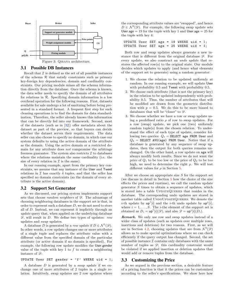
3. SYSTEM ARCHITECTUREIn this section, we describe the architecture of our pricing

system, depicted in Figure 3. Qirana is built as a layerthat sits on top of the DBMS. It consists of three distinctmodules: the support set generator and weight assignmentmodule are used in the preprocessing step (when the datais loaded, and the seller tunes the parameters), while thepricing module is used for interactive pricing. The runningexample throughout this section is the database of Figure 1.

DB

Support set generator module

Weight assignment module

Pricing moduleQ

p(Q,D)

Price points

Buyer Broker Seller

Figure 3: Qirana architecture.

3.1 Possible DB InstancesRecall that I is defined as the set of all possible instances

of the schema R that satisfy constraints such as primarykey-foreign key dependencies, domain and cardinality con-straints. Our pricing module mines all the schema informa-tion directly from the database. Once the schema is known,the data seller needs to specify the domain of all attributesfor relations in R. Specifying domain information is a lowoverhead operation for the following reasons. First, datasetsavailable for sale undergo a lot of sanitizing before being pre-sented in a standard format. A frequent first step for suchcleaning operations is to find the domain for data standard-ization. Therefore, the seller already knows this informationthat can be directly fed into our framework. Second, mostof the datasets (such as in [32]) offer metadata about thedataset as part of the preview, so that buyers can decidewhether the dataset serves their requirements. The dataseller can also choose to specify no domain, in which case oursystem defaults to using the active domain of the attributeas the domain. Using the active domain or a restricted do-main for any attribute does not compromise the arbitragefreeness guarantee. The system also restricts I to databaseswhere the relations maintain the same cardinality (i.e. thesize of every relation in I is the same).

In our running example, apart from the primary key con-straints, we assume that any instance of the User and Tweetrelations in I has exactly 4 tuples, and that the seller hasspecified no domain constraints (so the domain of every at-tribute is the active domain).

3.2 Support Set GeneratorAs we discussed, our pricing system implements support

sets that choose random neighbors of D . The advantage ofchoosing neighboring databases in the support set is that, inorder to represent such a databaseD, we do not need to storeall of D. Instead, we can represent it implicitly through anupdate query that, when applied on the underlying databaseD , will result in D. We define two types of updates: rowupdates and swap updates.

A database D is generated by a row update if D ∈ N 1(D).In other words, a row update changes one or more attributesof a single tuple and replaces the attribute value with adifferent value from the specified domain of the particularattribute (or active domain if no domain is specified). Forexample, the following row update modifies the User.gendervalue of the tuple with key 1 to f to create a neighboringinstance of D :

UPDATE User SET gender = ’f’ WHERE uid = 1;

A database D is generated by a swap update if we ex-change one of more attributes of 2 tuples in a single re-lation. Intuitively, swap updates are 2 row updates where

the corresponding attribute values are“swapped”, and henceD ∈ N 2(D). For example, the following swap update setsUser.age = 19 for the tuple with key 1 and User.age = 25 forthe tuple with key 4:

UPDATE User SET age = 19 WHERE uid = 1;UPDATE User SET age = 25 WHERE uid = 4;

Both row and swap updates always generate a new in-stance that is different from the original database D . Forevery update, we also construct an undo update that re-stores the affected row(s) to the original state. Our moduledecides which updates to apply (and hence what elementsof the support set to generate) using a random generator:

1. We choose the relation to be updated uniformly atrandom. In our running example, we will update Userwith probability 0.5 and Tweet with probability 0.5.

2. We choose each attribute (that is not the primary key)in the relation to be updated independently with prob-ability 0.5. Thus, the number of attributes that willbe modified are drawn from the geometric distribu-tion with p = 0.5. We do this to be more biased todatabases that will be “closer” to D .

3. We choose whether we have a row or swap update us-ing a predefined ratio ρ of row to swap updates. Fora row (swap) update, we pick one (two) uniformlyrandom tuple(s) from the chosen relation. To under-stand the effect of each type of update, consider fol-lowing two queries: Q1 = SELECT age FROM User andQ2 = SELECT AVG(age) FROM User. Notice that if adatabase is generated by any sequence of swap up-dates, then the output for both queries remains un-changed. On the other hand, a row update on age willalways modify both results. Since we do not want theprice of Q1 to be too low or the price of Q2 to be toohigh, we need to determine the right ρ. We will testdifferent values for ρ in Section 5.

After we choose an appropriate size S for the support set(we discuss in detail in Section 5 how the choice of the sizeeffects the prices and runtime), we call the random updategenerator S times to obtain a sequence of updates, whichis stored into a table UpdateQueries that resides in thedatabase. The corresponding undo updates are stored inanother table called UndoUpdateQueries. We denote thei-th update by up↑[i] and the i-th undo update by up↓[i],where i = 1, . . . , S. The i-the element of the support set isobtained as Di = up↑[i](D), and also D = up↓[i](Di).

Remark. We only use row and swap updates instead of awider class of updates (such as updates over multiple rows,insertions and deletions) for two reasons. First, as we willsee in Section 4.2, choosing updates that are from N 2(D)allows us to make special optimizations where we can checkefficiently if the query output has changed. Second, the setof possible instance I contains only databases with the samenumber of tuples as D ; this cardinality constraint wouldbe violated if we applied insertion or deletion updates thatwould add or remove tuples from the database.

3.3 Customizing the PriceAs we argued in the previous section, a desirable feature

of a pricing function is that it the prices can be customizedaccording to the seller’s specifications. We show here how

the weighted coverage function can be customized to reflectsuch choices. We emphasize that our technique does notapply to the other pricing functions, which is an argumentsupporting using weighted coverage as the default pricingfunction. Recall that the weighted coverage function assignsa weight wi to all instances Di ∈ S. The default way toassign these weights when the data seller has provided atthe minimum the price P of the full database is to assignequal weight wi = P/|S| to each instance in the support set.

Our framework allows the data seller to specify additionalprice points as a set of pairs (Qj , pj): this specifies thatfor any pricing function p that we compute, it must bethat p(Qj , D) = pj . For instance, the data seller in ourrunning example can specify that the price of the relationUser must be 70 using the price point (Q1, 70), where Q1 =SELECT * FROM User. The seller can also provide more fine-grained specifications about the pricing function, for exam-ple by pricing the attribute Car.age higher (with the pricepoint (SELECT uid, age FROM User, 50)), or by specifying(SELECT * FROM User WHERE ID = 4, 30).

Qirana can incorporate these price points into the priceby assigning different weights to the instances of the sup-port set. To choose the weights appropriately, we solve thefollowing (convex) entropy maximization(EM) problem:

maximize −|S|∑i=1

wi · log(wi)

subject to∑Di∈S

wi = P∑i:Qj(Di )=Qj(D)

wi = pj , j = 1, . . . , k

wi ≥ 0, i = 1, ..., |S|The first constraint encodes the fact that the price of thewhole dataset is P while the second constraint encodes theprice points. The objective maximizes the entropy of theweights, since under the presence of no additional informa-tion, we want to make the weights as uniform as possible(i.e. every part of the data equally valuable).

In our implementation, we solve this convex program us-ing the SCS conic solver [23] in CVXPY [14]. We shouldnote here that it is possible that the solver finds out thatthere exists no feasible solution for the given support setand the price points. In this case, we call the solver againafter we (a) resample the support set, or (b) increase the sizeof the support set. In such cases, SCS returns a certificate ofinfeasibility or unboundedness of the problem. However, thealgorithm returns optimal points to a modest objective ac-curacy when a solution exists. Hence, even though Qiranasupports arbitrary price points, in practice we restrict theprice points to be queries of two forms: selections over mul-tiple attributes, and projections. Based on our experience,we observed that with such restrictions, the solver could al-ways find a solution within one call when the number ofprice points was at most 11 per relation.

3.4 Computing the Pricing FunctionHere we will present how Qirana computes the price for

the pricing functions in Section 2.2. We will focus on thepricing algorithms for (a) weighted coverage, and (b) Shan-non entropy, since the computation for the uniform entropygain is similar to the weighted coverage, and for q-entropysimilar to Shannon entropy. Let Q = (Q1, Q2, . . . , Qk) bethe query bundle we want to price.

Weighted Coverage. Recall that the weighted coveragefunction computes the price as the weighted sum of the in-stances D in the support set for which Q(D) = Q(D). Qi-rana performs this computation using Algorithm 1. Thealgorithm initially computes the hash value of the outputQ(D) (line 3). Then, it iterates over the sequence of up-dates: for each update up↑[i], it applies the update to createa new databaseD (line 5), computes the hash value ofQ(D),and if it is different from the hash value of the original out-put, it adds wi to the price (line 7). Finally, it resets thedatabase to its original state by executing the correspondingundo update up↓[i] (line 8).

Algorithm 1: WeightedCoverage(Q)

1 price← 02 D ← D3 OUT ← h(Q(D))4 for i = 1, . . . , |S| do5 D ← up↑[i](D)6 if h(Q(D)) = OUT then7 price← price+ wi

8 D ← up↓[i](D)

9 return price

Shannon Entropy. In order to compute the price as theShannon entropy over the support set, we use a similar al-gorithm, depicted in Algorithm 2. The algorithm uses adictionary d to keep a weighted sum of the instances thathave the same hash value (line 5). When it has iterated overthe update sequence, it computes the entropy function basedon the dictionary values. The same algorithm can be usedto compute other entropy measures, with the only differencein the last line (where the output function is different).

Algorithm 2: ShannonEntropy(Q)

1 D ← D2 dict d← {}3 for i = 1, . . . , |S| do4 D ← up↑[i](D)5 d[h(Q(D))]← d[h(Q(D))] + wi

6 D ← up↓[i](D)

7 return −∑

b∈d.keys h[b] · log(h[b])

Both pricing algorithms have to run the query on the(modified) database as many times as the size of the supportset. This means that when the query runtime is slow, or thesupport set is too large, the time to compute the price willbe slow as well. To overcome this bottleneck, we observethat for Algorithm 1 we only need to check whether the up-date has modified the query output, and not actually runthe query. In Section 4 we exploit this observation to speedup the price computation by orders of magnitude.

3.5 Incorporating HistoryIn the previous section, we computed the price of a query

bundle while oblivious of the query history of the data buyer.We will show now how Qirana efficiently supports history-aware pricing while keeping a small memory footprint. Forsimplicity of exposition, we will discuss only the case for theweighted coverage pricing function, but our approach gener-alizes to any other pricing function. Suppose that the data

buyer has already issued queries Q1, . . . , Qk, which togetherform a bundle Q. In history-aware pricing, the buyer haspaid so far a total of p(Q,D) (instead of

∑j p(Qj ,D) in

the history-oblivious case). When a new query Qk+1 is is-sued, our pricing system must compute the new total priceas p(Q′,D), where Q′ is the bundle (Q1, . . . , Qk, Qk+1). De-fine:

Sk+1 = {D ∈ S | Q(D) = Q(D), Qk+1(D) = Qk+1(D)}.

Our key observation is that we express the new price asp(Q′,D) = p(Q,D) +

∑i:Di∈Sk+1

wj . In other words, our

history-aware pricing algorithm suffices to keep track of whichof the instances in S agree with D on all previous queries.Indeed, if at some point in the query history Di disagreedwith D , then Di has already contributed wj to the price, soit can be safely removed from the support set. If at somepoint every instance has disagreed with D , all future queriesare free for the buyer because the entire dataset has alreadybeen paid for.

The detailed history-aware pricing algorithm is presentedin Algorithm 3. The only bookkeeping that the algorithmneeds is a bitmap b that remembers which elements of thesupport set have already contributed to the price (bit setto 1), so they do not need to be considered anymore. No-tice that as the query history grows, computing the pricebecomes actually faster, since we need to consider less in-stances of the support set.

Algorithm 3: WeightedCoverage(Q) with history

1 b: bitmap that keeps history information2 price← 03 D ← D4 OUT ← h(Q(D))5 for i = 1, . . . , |S| do6 if b[i] = 0 then7 D ← up↑[i](D)8 if h(Q(D)) = OUT then9 price← price+ wi

10 b[i] = 1

11 D ← up↓[i](D)

12 return price

4. OPTIMIZING PRICE COMPUTATIONSAs we discussed in the previous section, the baseline pric-

ing algorithm that runs a queryQ on the (modified) databaseas many times as the size of the support set can be slow. Toovercome this issue, we exploit the fact that it suffices tocheck whether a given (row or swap) update modifies thequery output, instead of actually running the query. In thissection we present an algorithm that can tackle this problemefficiently for a large class of SQL queries.

Formally, given a database D, an update up↑, and a queryQ, the problem is to decide whether Q(D) = Q(up↑(D)),i.e. whether there exists a disagreement. This is a viewmaintenance problem, where the update is of a specific form,and we only check whether the output has changed insteadof maintaining the view. We first give the intuition aboutthe algorithm using our running example.

Example 4.1. Consider the query Q = SELECT * FROM

User WHERE age > 40 AND gender = ’m’. Consider the rowupdate up↑1 that sets the age of the tuple with key 3 to 30.

Since the updated tuple does not satisfy the predicate of Qanymore, the database D′ = up↑1(D) disagrees with D for the

query Q. Next, consider the row update up↑2 that modifies thegender of the tuple with key 4 to ′m′. It is not straightforwardto check if Q(up↑2(D)) agrees with Q(D) because we do notknow the age value for the tuple with uid = 4. In this case,we need additional information about all tuples t ∈ Q(D) todetermine if the view output changes or not, which we canobtain by issuing an ad hoc query.

We first consider the class of SPJ queries (queries with Se-lection, Projection, Join) without self-joins under bag (SQL)semantics. We then show how to extend our algorithm foraggregations.

4.1 Basic AlgorithmRecall that the database has schema R = (R1, . . . , Rk).

Let Pi denote the primary key of Ri. We can express anSPJ query Q in the following form in Relational Algebra:

Q = πA(σC(Ri1 × · · · ×Riℓ)) (5)

Here, A denotes the projected attributes in Q, and C is anarbitrary boolean expression over the attributes (which in-cludes both selection and join conditions). Given a tuple t inR, we denote by C[t] the new boolean expression that resultswhen we replace any attribute A of R in C with the valuet.A. We also need to transform Q to an augmented queryQ by including all primary keys Pi in the projection of theoutput for all relations Ri that participate in Q. Specifically,

Q = πPi1,...,Piℓ

,A(σC(Ri1 × · · · ×Riℓ)).

Our algorithm for checking disagreements for row updatesreturns True if we find a disagreement, otherwise False.This is a key difference between our setting and standardview maintenance, where the actual change on the outputresult needs to be computed. It will be convenient to de-scribe a row update up↑ as a pair of tuples (u−, u+) fromthe same relation R: we remove u− and subsequently addu+. By construction of the row updates, we will have thatu−.P = u+.P , where P is the primary key of R.

Algorithm 4: RowDisagree(Q,D, up↑)

1 up↑ = (u−, u+)2 R← updated relation3 P ← primary key of R4 B ← updated attributes of R5 if R ∈ {Ri1 , . . . , Riℓ} then6 return False

7 if u−.P ∈ πP (Q(D)) then8 if B ∩A = ∅ or C[u+] is unsatisfiable then9 return True

10 else11 if Q((D \R)∪{u−}) = Q((D \R)∪{u+}) then12 return True

13 else14 if Q((D \R) ∪ {u+}) = ∅ then15 return True

16 return False

Algorithm 4 first checks (line 5) whether the relation thatis modified by the update is involved in the query; if not,then we can safely say that the query result remains un-modified. Next, it checks (line 7) whether the tuple u− has

contributed to the output. If so, we check whether any ofthe updated attributes B are in the projected attributes A,or whether the new tuple u+ cannot participate in an an-swer because it makes C unsatisfiable. We know that inboth cases the output will certainly change. We should notehere that the unsatisfiability check for C[u+] in our imple-mentation is conservative for efficiency reasons (specifically,we check if the conditions that use only attributes of R be-come false). Also, observe that so far we perform the checks

statically given the output of Q (which we compute once),without running Q on every updated database.

If such a static check is not possible, we need to requestadditional information from the database (lines 11 and 14).In this case, we execute the query Q, but instead of runningthe query using the full relation R, we replace it with thesingleton {u+}. In practice, we implement this as a left outerjoin over the updated and original databases. The proof forthe correctness of Algorithm 4 can be found in Appendix A:

Theorem 4.1. Given a row update up↑ = (u−, u+) andan SPJ query Q, Algorithm 4 outputs False if Q(D) =Q(up↑(D)), otherwise it returns True.The case for swap updates is essentially the same,but withsome additional optimizations. The pseudocode for the algo-rithm SwapDisagree is presented in detail in Appendix A.

4.2 Batching UpdatesWe describe here a further optimization on the basic al-

gorithm presented in the previous section. RowDisagreespeeds up the computation in two ways. First, it can fil-ter out many possible updates from consideration withoutasking a query on the updated database. In practice, wenoticed that a large fraction of updates was evaluated thisway. Second, even if this is not the case, we can speed up thecomputation by running the query on the reduced databasesQ((D \ R) ∪ {u−}) and Q((D \ R) ∪ {u+}), for the updateup↑ = (u−, u+). However, we still need to run these queriesfor as many updates as necessary; even though computationwill be faster than Q(D), if we start with a large supportset, pricing may have a large overhead.

To overcome this problem, we batchmany such query com-putations together in a single query. Suppose that we have nrow updates up↑1, . . . , up

↑n over the same relation R, and the

algorithm needs to check whether Q((D\R)∪{u+i }) = ∅, for

i = 1, . . . , n. Let upid be an additional attribute that we useto keep the unique id of an update (which corresponds to an

element of the support set). Let i be the upid of up↑i for ourcase. We now create an instanceR+ = {(1, u+

1 ), . . . , (n, u+n )}

(we abuse the notation (i, u+i ) to mean that we append an

additional attribute upid to the tuple u+i ). R+ essentially

aggregates all the updates together in a single relation. LetD+ be the database that replaces R in D with R+, andQ the extended query that runs as Q, but projects the at-tribute upid as well. We next compute Q(D+) and observethe following: for any i = 1, . . . , n, Q((D \ R) ∪ {u+

i }) = ∅if and only if the output contains the upid with value i.

In general, for each relation R in the database we createthree batch queries. The one we just described correspondsto the check we do in line 14 of Algorithm 4. We need twomore batch queries for the check in line 11. The benefit ofbatching is that we only ask a constant number of querieson the database, independent of the size of the support set.Further, these queries will be much faster than Q(D), sincethe instances we run them on will be of smaller size.

4.3 AggregationWe present here an extension of our disagreement algo-

rithm for SPJ queries that supports SQL queries with ag-gregation and grouping. We consider queries of the form

Qγ = γG,agg1(A1),...,aggk(Ak)(Q)

where Q is an SPJ query, aggi are aggregation functions(SUM, COUNT, MIN, MAX, AVG), and G are the groupingattributes. Given a (row or swap) update up↑, recall thatour task is to check whether Qγ(D) = Qγ(up

↑(D)).We first describe our algorithm for the case of row up-

dates and aggregation that involves only COUNT; we willdiscuss how our technique can be generalized in the end ofthis section. For now, consider an aggregation query of theform Qγ = γG,COUNT(∗)(Q). Let Q◦

γ be the unrolled versionof the aggregation query, which removes the aggregation andprojects the relevant attributes: Q◦

γ = πG(Q). For exam-ple, the query γage,COUNT(∗)(User) on our running exampleis unrolled into the query πage(User).

The detailed approach is described in Algorithm 5. Noticethat to check whether the tuple u− of the update has con-tributed to the output, we need to compute the augmentedunrolled query Q◦

γ(D) (line 9). Now if the update modifiesany of the grouping attributes G, we know for sure that theoutput of the aggregate query will change, since the groupswill change. Similarly, if the new tuple u+ makes the se-lection or join conditions unsatisfiable, we know that thegroups where u− contributed will have their size reduced,and thus the output will again change. If none of these hap-pens, we have to go to the database and actually check ifQγ changes by running the query on the update database(line 13). Finally, if u− has not contributed to the out-put, we need to check whether u+ will do so (line 16). IfQ◦

γ((D \ R) ∪ {u+}) = ∅, then we know that the updatewill either add a new group, or increase the count of exist-ing group. Observe that for algorithm RowDisagreeAggit is not possible to batch the check of line 13 as with SPJqueries, but we can still batch the execution of line 16.

Algorithm 5: RowDisagreeAgg(Qγ , D, up↑)

1 Qγ = γG,COUNT(∗)(Q)2 Q◦

γ = πG(Q)

3 up↑ = (u−, u+)4 R← updated relation5 P ← primary key of R6 B ← updated attributes of R7 if R ∈ {Ri1 , . . . , Riℓ} then8 return False

9 if u−.P ∈ πP (Q◦γ(D)) then

10 if B ∩G = ∅ or C[u+] is unsatisfiable then11 return True12 else13 if Qγ(D) = Qγ((D \ {u−}) ∪ {u+}) then14 return True

15 else16 if Q◦

γ((D \R) ∪ {u+}) = ∅ then17 return True

18 return False

Theorem 4.2. Given a row update up↑ = (u−, u+) andan aggregate query Qγ = γG,COUNT(∗)(Q), where Q is an SPJ

query, Algorithm 5 outputs False if Qγ(D) = Qγ(up↑(D)),

otherwise it returns True.

The above algorithm can be slightly modified to also han-dle swap updates, in similar fashion to what we did withswap updates for SPJ queries. For aggregate queries involv-ing other types of aggregation functions, disagreements arecomputed in the same way as COUNT queries, except thatwe also need to keep track of the aggregate values of eachgroup in the output Qγ(D). For example, consider the caseof a query that has a MAX aggregate: γG,MAX(A)(Q), where

the unrolled query is πG,A(Q). Let up↑ be a row update forwhich, according to Algorithm 5, we need to check the con-dition in line 16. If Q◦

γ((D \ R) ∪ {u+}) = ∅, we know thatthe update has contributed some new tuples in the unrolledquery Q◦

γ . However, we can’t be sure that these new tupleswill change the output, since it could be that they belongin a group that has a larger maximum value. To overcomethis issue, we need to remember the maximum values fromQγ(D) and check the newly added tuples against the groupmaxima. The SUM aggregation works the same way. How-ever, if we know that all values in the aggregate column arestrictly positive, we can apply exactly Algorithm 5, withoutthe need to do any additional bookkeeping (since we knowthat the addition or removal of tuples will certainly changethe sum aggregate).

5. EXPERIMENTAL RESULTSWe have implemented our pricing framework in a tool

called Qirana in Python. We used MySQL (version 5.6.26)as the underlying DBMS that stores the data, but our ap-proach can work for any DBMS that supports SQL. We eval-uate Qirana on two aspects: (a) the behavior of the pricesassigned to queries, and (b) the runtime performance of thesystem for pricing queries on large datasets.

Benchmark Datasets. We perform our experimental eval-uation running queries over 5 real-world datasets in variousdomains (see Table 2 for a summary of their characteristics):

1. world: a popular database provided for developers. Ithas 3 relations: Country, City and CountryLanguage.

2. US Car crash 2011 [31]: A dataset about people in-volved in car accidents with fatalities available on Mi-crosoft Azure DataMarket.

3. DBLP [12]: describes a co-authorship network: 2 au-thors are connected if they have a publication together.

4. TPC-H [28]: a benchmark for performance metrics forsystems operating at a scale.

5. SSB [26]: a benchmark designed for measuring perfor-mance of classical data warehouse style workloads.

We use the world dataset to evaluate how prices are af-fected by support set size, as well as the fraction of rowto swap updates. The DBLP and US Car Crash datasets areused to show the prices of a range of queries in a real-worldsetting. The TPC-H and SSB datasets are used to evaluatethe scalability of our framework.

Experimental Setup. For all 5 datasets, we construct thesupport set assuming that the buyer knows the active do-main and cardinality of the relations. In order to assign theweights, we assume that the seller has provided no otherprice points apart from the total price of the dataset.

Qirana implements all four of the pricing functions inSection 2.3 with support set as random neighborhood around

dataset # relations # tuples # attributesworld 3 5, 302 21

US car crash 1 71, 115 14DBLP 1 1, 049, 866 2TPC-H 8 SF=1 61SSB 8 SF=1 56Table 2: Dataset characteristics.

D . In the following experiments we focus on the weightedcoverage function pwc unless explicitly stated. We madethis choice because the weighted coverage function is theonly pricing function that satisfies all three of the follow-ing properties: (a) it behaves well according to the bench-marking experiments in Section 2.4, (b) it is amenable tocustomization by using price points, and (c) it can be op-timized for performance using the techniques of Section 4.We further fix a 1 : 1 ratio of row to swap updates for allour experiments, unless explicitly mentioned. We run allour experiments on a single machine running OS X 10.10.5,equipped with 2.2GHz processor and 16GB RAM. For allperformance related experiments, we report the time aver-aged over 3 runs.

5.1 Effect of Framework ParametersWe first evaluate the behavior of prices according to differ-

ent choices of parameters. In particular, we study the effectof the support set size and the ratio of swap-row updates.

Varying Support Set Size. Figures 4a and 4b show theresult of executing the benchmark queries Qσ

u and Qπk (as

listed in Section 2.4) for varying support set size: 10, 100and 1000. The ideal price line plotted in both figures depictsthe price in the case where the support set is equal to thewhole set of neighboring databases. We can observe that forsmall values the resulting prices show high variability, sincethe support set does not cover the whole dataset well enough.Indeed, in the extreme where there exists one database in thesupport set, every query will have price either 0 or the priceof the full database. As the support set size increases, theprices for both selection and projection gradually convergeto the ideal price line. On the other hand, Figure 4d showsthat as the support set size increases, the computation re-quired to compute the price increases almost linearly. Thisexperiment shows the seller has a tradeoff space betweenperformance and how fine-grained the prices are, which shecan tune to her desires.

Varying Row to Swap Update Ratio. We next study theeffect of varying the ratio of row to swap updates. Considerthe following two queries:

Qr1: SELECT AVG(Population) FROM Country ;

Qr2: SELECT Name FROM Country WHERE

Population > 2 ,000 ,000 ,000 ;

For this experiment, we will assume that the buyer doesnot know the domain for Population, in which case a rowupdate can introduce a new value. In Figure 4c, we plotthe price of both queries when the fraction of swap updates(over the size of the support set) ranges from 0 to 1.

We can observe in Figure 4c that the price of both Qr1

and Qr2 is 0 when the fraction of swap updates is 1. This

happens because a swap update will never lead to any dis-agreement for any of the two queries. This is because everyswap will only exchange two values and the maximum valuefor Population in Country is 2, 000, 000, 000. This is not de-

1 32 64 128 239

u parameter in Q σu

0

20

40

60

80

100P

rice

10

100

1000

Ideal price

(a) σ−price vs selectivity

1 2 3 4 5 6 7 8 9 10 11 12 13

u parameter in Q πu

0

20

40

60

80

100

10

100

1000

Ideal price

(b) Π -price vs #attributes

0.00 0.25 0.50 0.75 1.00

fraction of swap updates

0

5

10

15

20Q r

1 Q r2

(c) price vs % of swaps

10 200 400 1000

Support Set size

0.0

0.1

0.2

0.3

0.4

Tim

e t

aken

in

s

Q σ80

Q π4

Q80

Q γ20

(d) time-support size tradeoff

Q1.1 Q1.2 Q1.3 Q2.1 Q2.2 Q2.3 Q3.1 Q3.2 Q3.3 Q3.4 Q4.1 Q4.2 Q4.3

Query

0

5

10

Pri

ce

history-oblivious

history-aware

(e) history aware pricing: SSB

Q1.1 Q1.2 Q1.3 Q2.1 Q2.2 Q2.3 Q3.1 Q3.2 Q3.3 Q3.4 Q4.1 Q4.2 Q4.3

Query

0

10

20

30

Tim

e i

n s

history-oblivious

history-aware

(f) history aware pricing: SSB

0 5 10 15 20 25

Query 1.1

0

5

10

Pri

ce

history-oblivious

history-aware

(g) history aware pricing: Q1.1

Figure 4: Experiments on the world and SSB datasets. The support set size in figures 4e, 4f, 4g is fixed to 100000, and infigure 4c to 1000.

Q1.1 Q1.2 Q1.3 Q2.1 Q2.2 Q2.3 Q3.1 Q3.2 Q3.3 Q3.4 Q4.1 Q4.2 Q4.3

Query

10-1

100

101

102

103

Tim

e i

n s

no batching

with batching

query execution time

(a) SSB scalability

Q1 Q2 Q4 Q5 Q6 Q11 Q12 Q17

Query

10-1

100

101

102

103

104

Tim

e i

n s

no batching with batching query execution time

(b) TPC-H scalability

Figure 5: Time in seconds to price SSB and TPCH queries on a support set of size 100000 without/with batching.

sirable, since when the user learns that the output of Qr2(D)

is empty, she has learned some information about the maxi-mum possible value of Population. Similarly, the output ofQr

1 discloses the average value.As the fraction of swap updates decreases, the prices of

both queries gradually increase. In the extreme that the sup-port set contains only row updates, all updates to Populationwill lead to a disagreement. This is also not desirable, be-cause the price of learning AVG(Population)($17 in our ex-periment) is close to price of learning the projecting of theentire column (in expectation, this would be $ 1

13100 if all

columns are uniformly valued). In our experience, an equalnumber of row and swap updates captures prices for aggre-gate queries best.

5.2 ScalabilityIn order to check how our algorithm scales, we evaluate

our system on the SSB and TPC-H datasets using a scalefactor of 1. As we mentioned in the beginning of the section,we price using only the weighted coverage function. Thesupport sets size for both datasets is set to S = 100, 000.

Our experimental results can be viewed in Figure 5a and5b for the SSB and TPC-H benchmarks respectively. We eval-uate the runtime performance for two different algorithms:the basic algorithm in Section 4.1, and the algorithm opti-mized to perform batch updates in Section 4.2. For refer-ence, we also report the time to execute the query Q on thedatabase D . We should note here that the time to compute

the price excludes the time to compute the query. Hence,we depict only the overhead of query pricing relative to thethe query computation time.

Our experiments show that with all optimizations acti-vated, we can price a query as fast (and sometimes faster)as the database can compute the query. Since the price com-putation involves asking queries over the database, a fasterDBMS would result in more efficient pricing. We can alsoobserve that the update batching optimization is critical tothe efficiency of our pricing algorithm, since the basic al-gorithm involves executing a query multiple times over thedata. Using batching makes pricing one to two orders ofmagnitude faster, since it avoids going to the database veryfrequently. For queries Q1.1-Q1.3 the price computation iseven faster, since the pricing algorithm does not need to runany queries on the database to check for disagreements.

5.3 History-Aware pricingFor queries in the SSB benchmark, we also evaluate history-

aware pricing to (a) observe the resulting prices assignedand (b) report the runtime when history-aware pricing isactivated. Figure 4f depicts the runtime for history-awarepricing when we run all 13 SSB queries in a sequence. Wecan observe that history-aware pricing is more efficient com-pared to the history-oblivious version. This is because ofthe decrease in the number of support set elements that weneed to consider at a later time. Figure 4e shows the pric-

Qd1 Qd

2 Qd3 Qd

4 Qd5 Qd

6

pwc+nbrs 2.07 0 4.29 0.29 0.045 58.82pH+nbrs 3.05 0 6.91 0.29 0.048 62.29

Qd7 Qc

1 Qc2 Qc

3 Qc4

pwc+nbrs 0.035 8.00 0.60 0.70 0pH+nbrs 0.038 9.03 0.58 0.76 0

Table 3: Prices for DBLP (Qdi ) and US Car crash (Qc

i )

ing savings for the same workload. Without history-awarepricing, a buyer would need to pay $12.14 instead of $6.94.

We observe similar behavior with parametrized queries. Inthe following, we generated 25 instances of query Q1.1 fromSSB with varying parameter values for dwdate, lo_discountand lo_quantity sampled uniformly from their domain. Fig-ure 4g shows the history-aware pricing for these queries. Thehistory-oblivious version forces the buyer to pay more than2× as compared to history-aware pricing.

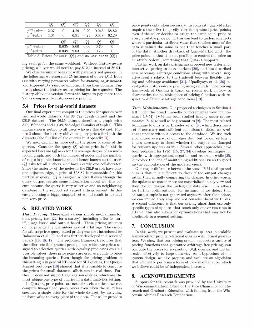
5.4 Prices for real-world datasetsOur final experiment computes the prices for queries over

two real world datasets: the US Car crash dataset and theDBLP dataset. The DBLP dataset describes a graph with317, 080 nodes and 1, 049, 866 edges (number of tuples). Thisinformation is public to all users who use this dataset. Fig-ure 3 shows the history-oblivious query prices for both thedatasets (the full list of the queries in Appendix B).

We next explain in more detail the prices of some of thequeries. Consider the query Qd

2 whose price is 0: this isexpected because Qd

2 asks for the average degree of an undi-rected graph, and both the number of nodes and the numberof edges is public knowledge and hence known to the user.Qd

6 asks for all authors who have exactly one collaborator.Since the majority of the nodes in the DBLP graph have onlyone adjacent edge, a price of $58.82 is reasonable for thisparticular query. Qc

4 is assigned a price 0 even though thequery output reveals some information about D : this oc-curs because the query is very selective and no neighboringdatabase in the support set caused a disagreement. In thiscase, choosing a bigger support set would result in a smallnon-zero price.

6. RELATED WORKData Pricing. There exist various simple mechanisms fordata pricing (see [22] for a survey), including a flat fee tar-iff, usage based and output based. These pricing schemesdo not provide any guarantees against arbitrage. The visionfor arbitrage free query-based pricing was first introduced byBalazinska et al. [3], and was further developed in a series ofpapers [16, 18, 17]. The proposed framework requires thatthe seller sets fine-grained price points, which are prices as-signed to selection queries with equality predicates over allpossible values; these price points are used as a guide to pricethe incoming queries. Even though the pricing problem inthis setting is in general NP-hard for SPJ queries, the Query-Market prototype [18] showed that it is feasible to computethe prices for small datasets, albeit not in real-time. Fur-ther, it does not support aggregation queries, which are themost ubiquitous type of queries in a data analytics setting.

InQirana, price points are not a first-class citizen; we cancompute fine-grained query prices even when the seller hasspecified a single price for the whole dataset, by assigninguniform value to every piece of the data. The seller provides

price points only when necessary. In contrast, QueryMarketrequires the seller to specify very fine-grained price points;even if the seller decides to assign the same equal price toevery available price point, this can lead to undesired effectswhere a particular attribute value that touches most of thedata is valued the same as one that touches a small partof the data. Another drawback of QueryMarket w.r.t. theprice points is that it is not possible to control the price onan attribute-level, something that Qirana supports.

Further work on data pricing has proposed new criteria forinteractive pricing in data markets [20], and has describednew necessary arbitrage conditions along with several neg-ative results related to the trade-off between flexible pric-ing and arbitrage avoidance [21]. Upadhyaya et al. [30] in-vestigates history-aware pricing using refunds. The pricingframework of Qirana is based on recent work on how tocharacterize the possible space of pricing functions with re-spect to different arbitrage conditions [13].

View Maintenance. Our proposed techniques in Section 4fall under the broad umbrella of incremental view mainte-nance (IVM). IVM has been studied heavily under set se-mantics [8, 6] as well as bag semantics [9]. The most relatedtechnique to ours is by Blakeley et al. [6], which describes aset of necessary and sufficient conditions to detect an irrel-evant update without access to the database. We use sucha condition as a part of our algorithm, but for our setting itis also necessary to check whether the output has changedfor relevant updates as well. Several other approaches havebeen proposed for IVM: [15, 27, 34] develops techniques forqueries with aggregation, negation and recursion while [25,2] explore the idea of maintaining additional views to speedup the computation of the updated views.

One major difference between the above IVM settings andours is that it is sufficient to check if the output changesrather than actually computing the change. In other words,the updates we consider are not materialized in any view andthey do not change the underlying database. This allowsfor further optimizations: for instance, if we detect thatan output tuple is not generated anymore after the update,we can immediately stop and not consider the other tuples.A second difference is that our pricing algorithms use onlyspecific types of updates that touch only one or two rows ina table: this also allows for optimizations that may not beapplicable in a general setting.

7. CONCLUSIONIn this work, we present and evaluate qirana, a scalable

framework for pricing relational queries with formal guaran-tees. We show that our pricing system supports a variety ofpricing functions that guarantee arbitrage-free pricing, cancompute the prices for a variety of SQL queries, and furtherscales effectively to large datasets. As a byproduct of oursystem design, we also propose and evaluate an algorithmthat efficiently performs a form of view maintenance, whichwe believe could be of independent interest.

8. ACKNOWLEDGMENTSSupport for this research was provided by the University

of Wisconsin-Madison Office of the Vice Chancellor for Re-search and Graduate Education with funding from the Wis-consin Alumni Research Foundation.

9. REFERENCES[1] S. Abiteboul and O. M. Duschka. Complexity of

answering queries using materialized views. In PODS,pages 254–263. ACM Press, 1998.

[2] Y. Ahmad, O. Kennedy, C. Koch, and M. Nikolic.Dbtoaster: Higher-order delta processing for dynamic,frequently fresh views. Proceedings of the VLDBEndowment, 5(10):968–979, 2012.

[3] M. Balazinska, B. Howe, and D. Suciu. Data marketsin the cloud: An opportunity for the databasecommunity. PVLDB, 4(12), 2011.

[4] Banjo. ban.jo.

[5] Big Data Exchange. www.bigdataexchange.com.

[6] J. A. Blakeley, N. Coburn, P. Larson, et al. Updatingderived relations: Detecting irrelevant andautonomously computable updates. ACMTransactions on Database Systems (TODS),14(3):369–400, 1989.

[7] Bloomberg Market Data. www.bloomberg.com/enterprise/content-data/market-data.

[8] O. P. Buneman and E. K. Clemons. Efficientlymonitoring relational databases. ACM Transactionson Database Systems (TODS), 4(3):368–382, 1979.

[9] S. Chaudhuri, R. Krishnamurthy, S. Potamianos, andK. Shim. Optimizing queries with materialized views.In Data Engineering, 1995. Proceedings of theEleventh International Conference on, pages 190–200.IEEE, 1995.

[10] N. N. Dalvi, C. Re, and D. Suciu. Probabilisticdatabases: diamonds in the dirt. Commun. ACM,52(7):86–94, 2009.

[11] DataFinder. datafinder.com.

[12] DBLP dataset.https://snap.stanford.edu/data/com-DBLP.html.

[13] S. Deep and P. Koutris. The design of arbitrage-freedata pricing schemes. arXiv preprintarXiv:1606.09376, 2016.

[14] S. Diamond and S. Boyd. CVXPY: APython-embedded modeling language for convexoptimization. Journal of Machine Learning Research,17(83):1–5, 2016.

[15] A. Gupta, I. S. Mumick, and V. S. Subrahmanian.Maintaining views incrementally. ACM SIGMODRecord, 22(2):157–166, 1993.

[16] P. Koutris, P. Upadhyaya, M. Balazinska, B. Howe,and D. Suciu. Query-based data pricing. InM. Benedikt, M. Krotzsch, and M. Lenzerini, editors,PODS, pages 167–178. ACM, 2012.

[17] P. Koutris, P. Upadhyaya, M. Balazinska, B. Howe,and D. Suciu. Querymarket demonstration: Pricing foronline data markets. PVLDB, 5(12):1962–1965, 2012.

[18] P. Koutris, P. Upadhyaya, M. Balazinska, B. Howe,and D. Suciu. Toward practical query pricing withquerymarket. In K. A. Ross, D. Srivastava, andD. Papadias, editors, ACMSIGMOD 2013, pages613–624. ACM, 2013.

[19] Lattice Data Inc. lattice.io.

[20] C. Li and G. Miklau. Pricing aggregate queries in adata marketplace. In WebDB, 2012.

[21] B. Lin and D. Kifer. On arbitrage-free pricing forgeneral data queries. PVLDB, 7(9):757–768, 2014.

[22] A. Muschalle, F. Stahl, A. Loser, and G. Vossen.Pricing approaches for data markets. In InternationalWorkshop on Business Intelligence for the Real-TimeEnterprise, pages 129–144. Springer, 2012.

[23] B. O’Donoghue, E. Chu, N. Parikh, and S. Boyd. SCS:Splitting conic solver, version 1.2.6.https://github.com/cvxgrp/scs, Apr. 2016.

[24] QLik Data Market.www.qlik.com/us/products/qlik-data-market.

[25] K. A. Ross, D. Srivastava, and S. Sudarshan.Materialized view maintenance and integrityconstraint checking: Trading space for time. In ACMSIGMOD Record, volume 25, pages 447–458. ACM,1996.

[26] SSB Benchmark.http://www.cs.umb.edu/˜poneil/StarSchemaB.PDF.

[27] M. Staudt and M. Jarke. Incremental maintenance ofexternally materialized views. In VLDB, volume 96,pages 3–6, 1996.

[28] TPC-H Benchmark. http://www.tpc.org/tpch.

[29] Twitter GNIP Audience API.gnip.com/insights/audience.

[30] P. Upadhyaya, M. Balazinska, and D. Suciu.Price-optimal querying with data apis. In PVLDB,2016.

[31] USA Car crash 2011 dataset. https://datamarket.azure.com/dataset/bigml/carcrashusa2011.

[32] Windows Azure Marketplace.www.datamarket.azure.com.

[33] world dataset.https://dev.mysql.com/doc/world-setup/en/.

[34] Y. Zhuge, H. Garcia-Molina, J. Hammer, andJ. Widom. View maintenance in a warehousingenvironment. ACM SIGMOD Record, 24(2):316–327,1995.

APPENDIXA. DETAILS FOR SECTION 4Correctness of Algorithm 4. We first need a basic resultover bag semantics.

Lemma A.1. Let E,F,G be bags. Then, E ∪ F = E ∪Gif and only if F = G.

Proof. For a bag S, let fS be a function that given avalue t returns its multiplicity in S. Since E ∪ F = E ∪ G,we can write that for every t, fE(t)+ fF (t) = fE(t)+ fG(t),which implies that fF (t) = fG(t). Hence, F = G.

Lemma A.2. Consider a database D, and a row updateup↑ = (u−, u+), where u− ∈ R. Then, Q(D) = Q(up↑(D))if and only if Q((D \R) ∪ {u−}) = Q((D \R) ∪ {u+}).

Proof. Let us denote D′′ = D\{u−}. We can now write:

Q(D′) = Q((D \ {u−}) ∪ {u+}) = Q(D′′) ∪Q((D \R) ∪ {u+})Q(D) = Q((D \ {u−}) ∪ {u−}) = Q(D′′) ∪Q((D \R) ∪ {u−})

where the last equality holds because union distributes overcartesian product, selection and projection. Notice that ifthe query includes only selection and projection over therelation R, then we simply have (D \R)∪{u+} = {u+}. Wecan apply now Lemma A.1 to obtain the desired result.

Proof of Theorem 4.1. Let P be the primary key forR. We distinguish the analysis to the following two cases:

1. u−.P ∈ πP (Q(D)): in this case, we know that u− didnot contribute to the output Q(D), and thus it mustbe that Q((D \ R) ∪ {u−}) = ∅. By Lemma A.2, itnow suffices to check whether Q((D \ R) ∪ {u+}) = ∅.Intuitively, if u+ now contributes to some output tuple,we are certain that the output will change.

2. u−.P ∈ πP (Q(D)): in this case, u− contributes to atleast one output tuple. If the new tuple u+ makes Cunsatisfiable, or any of the attributes modified are pro-jected, we are certain that the output will change. Ifnot and the query has no joins, we do not need to doanything further, since we can claim that the outputstays the same. In the case of joins, we need to fallback to running the query. By applying Lemma A.2,it suffices to run the query not on the whole database,but the one that replaces R with the singletons {u−}and {u+} respectively.

This concludes our correctness proof.

Computing Disagreements for Swap Updates. We showin detail the algorithm that checks for disagreements in thecase of a swap update (Algorithm 6). We denote a swap up-date as up↑ = (u−

1 , u+1 , u

+2 , u

+2 ), where all tuples come from

the same relation R. This update sequence removes u−1 , u

−2

and adds u+1 and u+

2 .

Algorithm 6: SwapDisagree(Q,D, up↑)

1 up↑ = (u−1 , u

+1 , u

+2 , u

+2 ) R← updated relation

2 P ← primary key of R3 B ← updated attributes of R4 if R ∈ {Ri1 , . . . , Riℓ} then5 return False

6 if u−1 .P and u−

2 .P /∈ πP (Q(D)) then7 if Q((D \R) ∪ {u+

1 , u+2 }) = ∅ then

8 return True

9 else10 if B ∩A = ∅ then11 return True

12 if C[u+2 ] and C[u+

1 ] are unsatisfiable then13 return True14 else15 if

Q((D \R)∪{u−1 , u

−2 }) = Q((D \R)∪{u+

1 , u+2 })

then16 return True

17 return False

Instance Reduction. We present here another optimiza-tion for price computation. This optimization replaces theinitial instanceD with a smaller instance based on the choiceof the support set S. In particular, we replace the instanceRi with a new relation R0

i by choosing from Ri only thetuples that are updated in S. Since a typical support size issmaller than the relation, R0

i will also be smaller in size. Wedenote the new database by D0

i (all other relations remainthe same). We will next show that we can run the basicalgorithm on any D0

i (instead of D), and obtain exactly thesame disagreements.

random D0 nbrs random

0

20

40

60

80

100

Pri

ce o

ut

of

100

(a) weighted coverage

coverage shannon entropy q-entropy uniform info gain

0

20

40

60

80

100

Pri

ce o

ut

of

10

0

(b) nbrs D support set

coverage shannon entropy q-entropy uniform info gain

0

20

40

60

80

100

Pri

ce o

ut

of

10

0

(c) uniform random support set

Figure 6: Additional benchmarking on world database

Lemma A.3. Let up↑ be a row or swap update that modi-fies Ri. Then, Q(D) = Q(up↑(D)) iff Q(D0

i ) = Q(up↑(D0i )).

Proof. Let us first consider a row update up↑ = (u−, u+)that updates Ri. From Lemma A.2, we know that Q(D) =Q((D \ {u−}) ∪ {u+}) if and only if Q((D \ Ri) ∪ {u−}) =Q((D \Ri) ∪ {u+}). But now for any tuple t, we have thatQ((D \ Ri) ∪ {t}) = Q((D0

i \ Ri) ∪ {t}). Thus, if we applyagain Lemma A.2, we will obtain that the desired resultholds if and only if Q(D0

i ) = Q(D0i \ {u−} ∪ {u+}). The

proof is similar for swap updates.

B. BENCHMARK QUERIESIn this section, we list all the queries used for pricing for

the real datasets. Queries for world, US car crash databsetand DBLP are listed in Table 7, 9 and 8 respectively.

We also performed additional benchmarking experimentto test the behavior of the pricing functions on a varietyof different queries on the world database (the full list ofqueries is in Appendix B). The results are plotted in Fig-ures 6a, 6b, 6c. We can see here the same behavior observedin our initial benchmark.

Query

Qw1 select count(Name) from Country where Continent = ‘Asia’

Qw2 select count(distinct Continent) from Country

Qw3 select avg(Population) from Country

Qw4 select max(Population) from Country

Qw5 select min(LifeExpectancy) from Country

Qw6 select count(Name) from Country where Name like ‘A

Qw7 select Region, max(SurfaceArea) from Country group by Region

Qw8 select Continent, max(Population) from Country group by Continent

Qw9 select Continent, count(Code) from Country group by Continent

Qw10 select * from Country

Qw11 select Name from Country where Name like ’A%’

Qw12 select * from Country where Continent=’Europe’ and Population > 5000000

Qw13 select * from Country where Region=’Caribbean’

Qw14 select Name from Country where Region=’Caribbean’

Qw15 select Name from Country where Population between 10000000 and 20000000

Qw16 select * from Country where Continent=’Europe’ limit 2

Qw17 select Population from Country where Code = USA’

Qw18 select GovernmentForm from Country

Qw19 select distinct GovernmentForm from Country

Qw20 select * from City where Population >= 1000000 and CountryCode = ’USA’

Qw21 select distinct Language from CountryLanguage where CountryCode=’USA’

Qw22 select * from CountryLanguage where IsOfficial = ’T’ ’

Qw23 select Language, count(CountryCode) from CountryLanguage group by Language

Qw24 select count(Language) from CountryLanguage where CountryCode = ’USA’

Qw25 select CountryCode, sum(Population) from City group by CountryCode

Qw26 select CountryCode, count(ID) from City group by CountryCode

Qw27 select * from City where CountryCode = ’GRC’

Qw28 select distinct 1 from City where CountryCode = ’USA’ and Population > 10000000

Qw29 select Name from Country , CountryLanguage where Code = CountryCode and Language = ’Greek’

Qw30

select C.Name from Country C, CountryLanguage L where C.Code = L.CountryCode and L.Language =

’English’ and L.Percentage >= 50

Qw31 select T.district from Country C, City T where C.code = ’USA’ and C.capital = T.id

Qw32

select * from Country C, CountryLanguage L where C.Code = L.CountryCode and L.Language =

’Spanish’

Qw33 select Name, Language from Country , CountryLanguage where Code = CountryCode

Qw34 select * from Country , CountryLanguage where Code = CountryCode

Figure 7: Queries used for world database

Query

Qd1 select FromNodeId, count(ToNodeId) from dblp group by FromNodeId having count(ToNodeId) > 100

Qd2

select avg(cnt) from (select FromNodeId, count(ToNodeId) as cnt from dblp group by FromNodeId )

as rc

Qd3 select count(*) from dblp A where FromNodeId > 10000

Qd4

select FromNodeId, count(*) from dblp A where A.FromNodeId in (select FromNodeId from dblp B

where B.ToNodeId = 38868) group by FromNodeId

Qd5 select ToNodeId from dblp where (FromNodeId = 148255 or FromNodeId = 45479)

Qd6 select FromNodeId, count(*) as collab from dblp group by ToNodeId having collab = 1

Qd7 select * from dblp A where A.FromNodeId = 38868 or A.ToNodeId = 38868

Figure 8: Queries used for DBLP database

Query

Qc1 select state, count(*) from crash group by State

Qc2 select count(*) from crash where State = ’Texas’ and Gender = ’Male’ and Alcohol_Results > 0.0

Qc3

select sum(Fatalities_in_crash) from crash where State = ’California’ and Crash_Date >= date

’2011-01-01’ and Crash_Date < date ’2011-01-01’ + interval ’6’ month

Qc4

select count(Fatalities_in_crash) from crash where State = ’Wisconsin’ and Injury_Severity =

’Fatal Injury (K)’ and (Atmospheric_Condition = ’Snow’)

Figure 9: Queries used for US car crash dataset