QInfer: Statistical inference software for quantumapplicationsChristopher Granade1 2, Christopher Ferrie3, Ian Hincks4 5, Steven Casagrande, Thomas Alexander5 6,Jonathan Gross7, Michal Kononenko5 6, and Yuval Sanders5 6 8

1 School of Physics, University of Sydney, Sydney, NSW, Australia2 Centre for Engineered Quantum Systems, University of Sydney, Sydney, NSW, Australia3 University of Technology Sydney, Centre for Quantum Software and Information, Ultimo NSW 2007, Australia4 Department of Applied Mathematics, University of Waterloo, Waterloo, ON, Canada5 Institute for Quantum Computing, University of Waterloo, Waterloo, ON, Canada6 Department of Physics and Astronomy, University of Waterloo, Waterloo, ON, Canada7 Center for Quantum Information and Control, University of New Mexico, Albuquerque, NM 87131-0001, USA8 Department of Physics and Astronomy, Macquarie University, Sydney, NSW, Australia

April 14, 2017

Characterizing quantum systems through ex-perimental data is critical to applications asdiverse as metrology and quantum computing.Analyzing this experimental data in a robustand reproducible manner is made challenging,however, by the lack of readily-available soft-ware for performing principled statistical anal-ysis. We improve the robustness and repro-ducibility of characterization by introducing anopen-source library, QInfer, to address thisneed. Our library makes it easy to analyzedata from tomography, randomized benchmark-ing, and Hamiltonian learning experiments ei-ther in post-processing, or online as data is ac-quired. QInfer also provides functionality forpredicting the performance of proposed experi-mental protocols from simulated runs. By deliv-ering easy-to-use characterization tools based onprincipled statistical analysis, QInfer helps ad-dress many outstanding challenges facing quan-tum technology.

Contents1 Introduction 1

2 Inference and Particle Filtering 2

Christopher Granade: cgranade@cgranade.com, www.cgranade.com

Complete source code available at DOI 10.5281/zenodo.157007.

3 Applications in Quantum Information 43.1 Phase and Frequency Learning . . . . . 43.2 State and Process Tomography . . . . . 53.3 Randomized Benchmarking . . . . . . . 7

4 Additional Functionality 74.1 Region Estimation and Error Bars . . . . 74.2 Derived Models . . . . . . . . . . . . . . 84.3 Time-Dependent Models . . . . . . . . . 94.4 Performance and Robustness Testing . . 104.5 Parallelization . . . . . . . . . . . . . . . 114.6 Other Features . . . . . . . . . . . . . . . 13

5 Conclusions 14

Acknowledgments 14

References 14

A Custom Model Example 17

B Resampling 17

1 IntroductionStatistical modeling and parameter estimation play acritical role in many quantum applications. In quan-tum information in particular, the pursuit of large-scale quantum information processing devices has mo-tivated a range of different characterization protocols,and in turn, new statistical models. For example, quan-tum state and process tomography are widely usedto characterize quantum systems, and are in essence

1

arX

iv:1

610.

0033

6v2

[qu

ant-

ph]

13

Apr

201

7

matrix-valued parameter estimation problems [1, 2].Similarly, randomized benchmarking is now a main-stay in assessing quantum devices, motivating the useof rigorous statistical analysis [3] and algorithms [4].Quantum metrology, meanwhile, is intimately con-cerned with what parameters can be extracted frommeasurements of a physical system, immediately ne-cessitating a statistical view [5, 6].

The prevalence of statistical modeling in quantumapplications should not be surprising: quantum me-chanics is an inherently statistical theory, thus infer-ence is an integral part of both experimental and theo-retical practice. In the former, experimentalists need tomodel their systems and infer the value of parametersfor the purpose of improving control as well as validat-ing performance. In the latter, numerical experimentsutilizing simulated data are now commonplace in the-oretical studies, such that the same inference problemsare encountered usually as a necessary step to answerquestions about optimal data processing protocols orexperiment design. In both cases, we lack tools torapidly prototype and access inference strategies; QIn-fer addresses this need by providing a modular inter-face to a Monte Carlo algorithm for performing statis-tical inference.

Critically, in doing so, QInfer also supports and en-ables open and reproducible research practices. Par-allel to the challenges faced in many other disciplines[7], physics research cannot long survive its own cur-rent practices. Open access, open source, and opendata provide an indispensable means for research to bereproducible, ensuring that research work is useful tothe communities invested in that research [8]. In theparticular context of quantum information research,open methods are especially critical given the impactof statistical errors that can undermine the claims ofpublished research [9, 10]. Ensuring the reproducibil-ity of research is critical for evaluating the extent towhich statistical and methodological errors underminethe credibility of published research [11].

QInfer also constitutes an important step towards amore general framework for quantum verification andvalidation (QCVV). As quantum information proces-sor prototypes become more complex, the challengeof ensuring that noise processes affecting these de-vices conform to some agreed-upon standard becomesmore difficult. This challenge can be managed, at leastin principle, by developing confidence in the truth ofcertain simplifying assumptions and approximations.The value of randomized benchmarking, for example,depends strongly upon the extent to which noise isapproximately Pauli [12]. QInfer provides a valuableframework for the design of automated and efficientnoise assessment methods that will enable the compar-

ison of actual device performance to the specificationsdemanded by theory.

To the end of enabling reproducible and accessibleresearch, and hence providing a reliable process for in-terpreting advances in quantum information process-ing, we base QInfer using openly-available tools suchas the Python programming language, the IPython in-terpreter, and Jupyter [13, 14]. Jupyter in particularhas already proven to be an invaluable tool for repro-ducible research, in that it provides a powerful frame-work for describing and explaining research software[15]. We provide our library under an open-source li-cense along with examples [16] of how to use QInfer tosupport reproducible research practices. In this way,our library builds on and supports recent efforts to de-velop reproducible methods for physics research [17].

QInfer is a mature open-source software library writ-ten in the Python programming language which hasnow been extensively tested in a wide range of infer-ential problems by various research groups. Recogniz-ing its maturity through its continuing development,we now formally release version 1.0. This maturity hasgiven its developers the opportunity to step back andfocus on the accessibility of QInfer such that other re-searchers can benefit from its utility. This short paperis the culmination of that effort. A full Users’ Guide isavailable in the ancillary files.

We proceed as following. In Section 2, we give abrief introduction to Bayesian inference and particle fil-tering, the numerical algorithm we use to implementBayesian updates. In Section 3, we describe applica-tions of QInfer to common tasks in quantum informa-tion processing. Next, we describe in Section 4 addi-tional features of QInfer before concluding in Section 5.

2 Inference and Particle FilteringQInfer is primarily intended to serve as a toolset forimplementing Bayesian approaches to statistical infer-ence. In this section, we provide a brief review of theBayesian formalism for statistical inference. This sec-tion is not intended to be comprehensive; our aim israther to establish the language needed to describe theQInfer codebase.

In the Bayesian paradigm, statistical inference is theprocess of evaluating data obtained by sampling anunknown member of a family of related probabilitydistributions, then using these samples to assign a rel-ative plausibility to each distribution. Colloquially, wethink of this family of distributions as a model param-eterized by a vector x of model parameters. We thenexpress the probability that a dataset D was obtainedfrom the model parameters x as Pr(D|x) and read it as

2

“the probability of D given that the model specified byx is the correct model.” The function Pr(·|x) is calledthe likelihood function, and computing it is equivalentto simulating an experiment1. For example, the Bornrule is a likelihood function, in that it maps a known orhypothetical quantum density matrix x ≡ ρ to a distri-bution over measurement outcomes of a measurementD ∈ {E,1−E} via

Pr(D = E|x) = Tr(Eρ). (1)

The problem of estimating model parameters is asfollows. Suppose an agent is provided with a datasetD and is tasked with judging the probability that themodel specified by a given vector x is in fact the correctone. According to Bayes’ rule,

Pr(x|D) =Pr(D|x)Pr(x)

Pr(D), (2)

where Pr(x) is a probability distribution called theprior distribution and Pr(x|D) is called the posteriordistribution. If the agent is provided with a priordistribution, then they can estimate parameters usingBayes’ rule. Note that Pr(D) can be computed throughmarginalization, which is to say that the value can inprinciple be calculated via the equation

Pr(D) =

∫x

Pr(D|x)Pr(x)dx. (3)

For the inference algorithm used by QInfer, Pr(D) isan easily computed normalization constant and thereis no need to compute a possibly complicated integral.

Importantly, we will demand that the agent’s dataprocessing approach works in an iterative manner.Consider the example in which the data D is in facta set D = {d1, . . . , dN} of individual observations. Inmost if not all classical applications, each individualdatum is distributed independently of the rest of thedata set, conditioned on the true state. Formally, wewrite that for all j and k such that j 6= k, dj ⊥ dk | x.This may not hold in quantum models where measure-ment back-action can alter the state. In such cases, wecan simply redefine what the parameters x label, suchthat this independence property can be taken as a con-vention, instead of as an assumption. Then, we havethat

Pr(x|d1, . . . , dN ) =Pr(dN |x)Pr(x|d1, . . . , dN−1)

Pr(dN ).

(4)

1Here, we use the word “simulation” in the sense of what Vanden Nest [18] terms “strong simulation,” as opposed to drawingdata consistent with a given model (“weak simulation”).

In other words, the agent can process the data sequen-tially where the prior for each successive datum is theposterior from the last.

This Bayes update can be solved analytically in someimportant special cases, such as frequency estimation[19, 20], but is more generally intractable. Thus, to de-velop a robust and generically useful framework forparameter estimation, the agent relies on numerical al-gorithms. In particular, QInfer is largely concernedwith the particle filtering algorithm [21], also knownas the sequential Monte Carlo (SMC) algorithm. Inthe context of quantum information, SMC was firstproposed for learning from continuous measurementrecords [22], and has since been used to learn fromstate tomography [23], Hamiltonian learning [24], andrandomized benchmarking [4], as well as other appli-cations.

The aim of particle filtering is to replace a continuousprobability distribution Pr(x) with a discrete approxi-mation ∑

k

wkδ(x−xk), (5)

where w = (wk) is a vector of probabilities. The entrywk is called the weight of the particle, labeled k, and xkis the location of particle k.

Of course, the particle filter∑k wkδ(x − xk) does

not directly approximate Pr(x) as a distribution; theparticle filter, if considered as a distribution, is sup-ported only a discrete set of points. Instead, the par-ticle filter is used to approximate expectation values: iff is a function whose domain is the set of model vec-tors x, we want the particle filter to satisfy∫

f(x)Pr(x)dx ≈∑k

wkf(xk). (6)

The posterior distribution can also be approximatedusing a particle filter. In fact, a posterior particle filtercan be computed directly from a particle filter for theprior distribution as follows. Let {(wk,xk)} be the setof weights and locations for a particle filter for someprior distribution Pr(x). We then compute a particlefilter {(w′k,x′k)} for the posterior distribution by set-ting x′k = xk and

w′k =wk Pr(D|xk)∑j wj Pr(D|xj)

, (7)

whereD is the data set used in the Bayesian update. Inpractice, updating the weights in this fashion causesthe particle filter to become unstable as data is col-lected; by default, QInfer will periodically apply theLiu–West algorithm to restore stability [25]. See Ap-pendix B for details.

3

At any point during the processing of data, the ex-pectation of any function with respect to the posterioris approximated as

E[f(x)|D] ≈∑k

wk(D)f(xk). (8)

In particular, the expected error in x is given bythe posterior covariance, Cov(x|D) := E[xxT|D] −E[x|D]ET[x|D]. This can be used, for instance, toadaptively choose experiments which minimize theposterior variance [24]. This approach has been usedto exponentially improve the number of samples re-quired in frequency estimation problems [19, 20], andin phase estimation [26, 27]. Alternatively, other costfunctions can be considered, such as the informationgain [23, 28]. QInfer allows for quickly computing ei-ther the expected posterior variance or the informa-tion gain for proposed experiments, making it straight-forward to develop adaptive experiment design proto-cols.

The functionality exposed by QInfer follows a sim-ple object model, in which the experiment is describedin terms of a model, and background information is de-scribed in terms of a prior distribution. Each of theseclasses is abstract, meaning that they define what be-havior a QInfer user must specify in order to fullyspecify an inference procedure. For convenience, QIn-fer provides several pre-defined implementations ofeach, as we will see in the following examples. Con-crete implementations of a model and a prior distribu-tion are then used with SMC to update the prior basedon data. In summary, the iterative approach describedabove is formalized in terms of the following Pythonobject model:

class qinfer.Distribution:

abstract sample(n): Returns n samples fromthe represented distribution.

class qinfer.Model:

abstract likelihood(d, x, e): Returns an evalu-ation of the likelihood function Pr(d|x; e) fora single datum d, a vector of model parame-ters x and an experiment e.

abstract are models valid(x): Evaluateswhether x is a valid assignment of modelparameters.

class qinfer.SMCUpdater:

update(d, e): Computes the Bayes update (7) fora single datum (that is, D = {d}).

est mean(): Returns the current estimate x =E[x].

A complete description of the QInfer object modelcan be found in the Users’ Guide. Notablyqinfer .SMCUpdater relies only on the behavior specifiedby each of the abstract classes in this object model.Thus, it is straightforward for the user to specifytheir own prior and likelihood function by either im-plementing these classes (as in the example of Ap-pendix A), or by using one of the many concrete im-plementations provided with QInfer.

The concrete implementations provided with QIn-fer are useful in a range of common applications, as de-scribed in the next Section. We will demonstrate howthese classes are used in practice with examples drawnfrom quantum information applications. We will alsoconsider the qinfer .Heuristic class, which is useful in con-texts such as online adaptive experiments and simu-lated experiments.

3 Applications in Quantum InformationIn this Section, we describe various possible applica-tions of QInfer to existing experimental protocols. Indoing so, we highlight both functionality built-in toQInfer and how this functionality can be readily ex-tended with custom models and distributions. We be-gin with the problems of phase and frequency learning,then describe the use of QInfer for state and process to-mography, and conclude with applications to random-ized benchmarking.

3.1 Phase and Frequency LearningOne of the primary applications for particle filtering isfor learning the Hamiltonian H under which a quan-tum system evolves [24]. For instance, consider thesingle-qubit Hamiltonian H = ωσz/2 for an unknownparameter ω. An experiment on this qubit may thenconsist of preparing a state |+〉 = (|0〉 + |1〉)/

√2,

evolving for a time t and then measuring in the σx ba-sis. This model commonly arises from Ramsey inter-ferometry, and gives a likelihood function

Pr(0|ω; t) =∣∣ 〈+| e−iωtσz/2 |+〉

∣∣2= cos2(ωt/2).

(9)

Note that this is also the same model for Rabi inter-ferometry as well, with the interpretation ofH as driveterm rather than the internal Hamiltonian for a system.Similarly, this model forms the basis of Bayesian andmaximum likelihood approaches to phase estimation.

In any case, QInfer implements (9) as theSimplePrecessionModel class, making it easy to quicklyperform Bayesian inference for Ramsey or Rabi esti-mation problems. We demonstrate this in Listing 1,

4

0 20 40 60 80 100

# of Experiments Performed

0.4

0.5

0.6

0.7

0.8

0.9

ω

Est. True

Figure 1: Frequency estimate obtained using Listing 1 as a function of the number of experiments performed.

using ExpSparseHeuristic to select the kth measurement time tk = (9/8)k, as suggested by analytic arguments[19].

Listing 1: Frequency estimation example using SimplePrecessionModel.>>> from q i n f e r import *>>> model = SimplePrecessionModel ( )>>> p r i o r = UniformDistr ibut ion ( [ 0 , 1 ] )>>> n p a r t i c l e s = 2000

5 >>> n experiments = 100>>> updater = SMCUpdater ( model , n p a r t i c l e s , p r i o r )>>> h e u r i s t i c = ExpSparseHeurist ic ( updater )>>> true params = p r i o r . sample ( )>>> for idx experiment in range ( n experiments ) :

10 . . . experiment = h e u r i s t i c ( ). . . datum = model . s imulate experiment ( true params , experiment ). . . updater . update ( datum , experiment )>>> print ( updater . est mean ( ) )

More complicated models for learning Hamiltonianswith particle filtering have also been considered [29–32]; these can be readily implemented in QInfer as cus-tom models by deriving from the Model class, as de-scribed in Appendix A.

3.2 State and Process Tomography

Though originally conceived of as a algebraic inverseproblem, quantum tomography is also a problem ofparameter estimation. Many have also considered theproblem in a Bayesian framework [33, 34] and the se-quential Monte Carlo algorithm has been used in boththeoretical and experimental studies [23, 28, 35–37].

To define the model, we start with a basis for trace-less Hermitian operators {Bj}d

2−1j=1 . In the case of a

qubit, this could be the basis of Pauli matrices, for ex-

ample. Then, any state ρ can be written

ρ =1

d+d2−1∑j=1

θjBj , (10)

for some vector of parameters θ. These parametersmust be constrained such that ρ ≥ 0.

In the simplest case, we can consider two-outcomemeasurements represented by the pair {E,1−E}. TheBorn rule defines the likelihood function

Pr(E|ρ) = Tr(ρE). (11)

For multiple measurements, we simply iterate. Formany trials of the same measurement, we can use aderived model as discussed below.

QInfer’s TomographyModel abstracts many of the im-plementation details of this problem, exposing tomo-graphic models and estimates in terms of QuTiP’s Qobj

5

1 0 1

Tr(σxρ)

1

0

1

Tr(σzρ)

Credible Region (α= 0. 95)

Posterior

True

Posterior Mean

Figure 2: Posterior over rebit states after 100 random Pauli measurements, each repeated five times, as implemented by Listing 2.

class [38]. This allows for readily integrating QIn-fer functionality with that of QuTiP, such as fidelitymetrics, diamond norm calculation, and other suchmanipulations.

Tomography support in QInfer requires one of the

bases mentioned above in order to parameterize thestate. Many common choices of basis are included asTomographyBasis objects, such as the Pauli or Gell-Mannbases. Many of the most commonly used priors are al-ready implemented as a QInfer Distribution.

Listing 2: Rebit state tomography example using TomographyModel.>>> from q i n f e r import *>>> from q i n f e r . tomography import *>>> b a s i s = p a u l i b a s i s ( 1 ) # Single−qubit Paul i b a s i s .>>> model = TomographyModel ( b a s i s )

5 >>> p r i o r = G i n i b r e R e d i t D i s t r i b u t i o n ( b a s i s )>>> updater = SMCUpdater ( model , 8000 , p r i o r )>>> h e u r i s t i c = RandomPauliHeuristic ( updater )>>> t r u e s t a t e = p r i o r . sample ( )>>>

10 >>> for idx experiment in range ( 5 0 0 ) :>>> experiment = h e u r i s t i c ( )>>> datum = model . s imulate experiment ( t r u e s t a t e , experiment )>>> updater . update ( datum , experiment )

For simulations, common randomized measure-ment choices are already implemented. For exam-ple, RandomPauliHeuristic chooses random Pauli mea-surements for qubit tomography.

In Listing 2, we demonstrate QInfer’s tomographysupport for a rebit. By analogy to the Bloch sphere, arebit may be represented by a point in the unit disk,making rebit tomography useful for plotting exam-ples. More generally, with different choices of basis,QInfer can be used for qubits or higher-dimensionalstates. For example, recent work has demonstrated theuse of QInfer for tomography procedures on seven-dimensional states [39]. Critically, QInfer provides aregion estimate for this example, describing a region thathas a 95% probability of containing the true state. We

will explore region estimation further in Section 4.1.

Finally, we note that process tomography is a spe-cial case of state tomography [36], such that the samefunctionality described above can also be used to ana-lyze process tomography experiments. In particular,the qinfer .ProcessTomographyHeuristic class represents theexperiment design constraints imposed by process to-mography, while BCSZChoiDistribution uses the distribu-tion over completely positive trace-preserving mapsproposed by Bruzda et al. [40] to represent a prior dis-tribution over the Choi states of random channels.

6

3.3 Randomized BenchmarkingIn recent years, randomized benchmarking (RB) hasreached a critical role in evaluating candidate quantuminformation processing systems. By using random se-quences of gates drawn from the Clifford group, RBprovides a likelihood function that depends on the fi-delity with which each Clifford group element is im-plemented, allowing for estimates of that fidelity to bedrawn from experimental data [4].

In particular, suppose that each gate is implementedwith fidelity F , and consider a fixed initial state andmeasurement. Then, the survival probability over se-quences of length m is given by [41]

Pr(survival|p,A,B;m) = Apm +B, (12)

where p := (dF − 1)/(d− 1), d is the dimension of thesystem under consideration, and where A and B de-scribe the state preparation and measurement (SPAM)errors. Learning the modelx = (p,A,B) thus provides

an estimate of the fidelity of interest F .The likelihood function for randomized benchmark-

ing is extremely simple, and requires only scalararithmetic to compute, making it especially usefulfor avoiding the computational overhead typically re-quired to characterize large quantum systems withclassical resources. Multiple generalizations of RBhave been recently developed which extend these ben-efits to estimating crosstalk [42], coherence [43], and toestimating fidelities of non-Clifford gates [44, 45]. RBhas also been extended to provide tomographic infor-mation as well [46]. The estimates provided by ran-domized benchmarking have also been applied to de-sign improved control sequences [47, 48].

QInfer supports RB experiments through theqinfer .RandomizedBenchmarkingModel class. For commonpriors, QInfer also provides a simplified interface,qinfer .simple est rb, that reports the mean and covarianceover an RB model given experimental data. We pro-vide an example in Listing 3.

Listing 3: Randomized benchmarking example using simple est rb .>>> from q i n f e r import *>>> import numpy as np>>> p , A, B = 0 . 9 5 , 0 . 5 , 0 . 5>>> ms = np . l i n s p a c e ( 1 , 800 , 2 0 1 ) . astype ( i n t )

5 >>> s i g n a l = A * p * * ms + B>>> n shots = 25>>> counts = np . random . binomial ( p=s ignal , n=n shots )>>> data = np . column stack ( [ counts , ms , n shots * np . o n e s l i k e ( counts ) ] )>>> mean , cov = s i m p l e e s t r b ( data , n p a r t i c l e s =12000 , p min = 0 . 8 )

10 >>> print ( mean , np . s q r t ( np . diag ( cov ) ) )

4 Additional FunctionalityHaving introduced common applications for QInfer, inthis Section we describe additional functionality whichcan be used with each of these applications, or withcustom models.

4.1 Region Estimation and Error BarsAs an alternative to specifying the entire posterior dis-tribution approximated by qinfer .SMCUpdater, we pro-vide methods for reporting credible regions over theposterior, based on covariance ellipsoids, convex hulls,and minimum volume enclosing ellipsoids [35]. Theseregion estimators provide a rigorous way of summa-rizing one’s uncertainty following an experiment (col-loquially referred to as “error bars”), and owing to theBayesian approach, do so in a manner consistent withexperimental experience.

Posterior credible regions can be found by usingthe SMCUdater.est credible region method. This methodreturns a set of particles such that the sum of theirweights corresponding weights is at least a specified

ratio of the total weight. For example, a 95% credibleregions is represented as a collection of particles whoseweight sums to at least 0.95.

This does not necessarily admit a very compact de-scription since many of the particles would be interiorto the regions. In such cases, it is useful to find regionestimators containing all of the particles describing acredible region. The SMCUpdater.region est hull methoddoes this by finding a convex hull of the credible parti-cles. Such a hull is depicted in Figure 2.

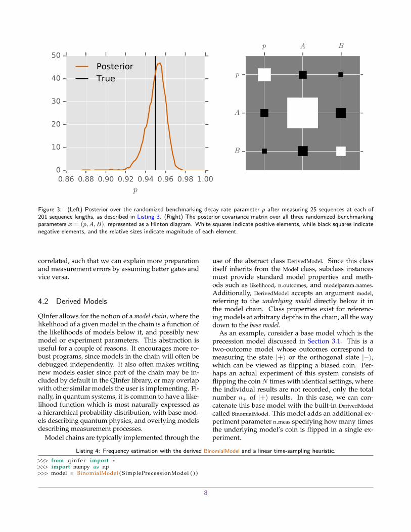
The convex hull of an otherwise random set of pointsis also not necessarily easy to describe or intuit. In suchcases, SMCUdpater.region est ellipsoid finds the minimum-volume enclosing ellipse (MVEE) of the convex hullregion estimator. As the name suggests, this is thesmallest ellipsoid containing the credible particles. Itis strictly larger than the hull and thus maintains cred-ibility. Ellipsoids are specified by their center andcovariance matrix. Visualizing the covariance ma-trix can also usually provide important diagnostic in-formation, as in Figure 3. In that example, we canquickly see that the p and A parameters estimatedfrom a randomized benchmarking experiment are anti-

7

0.86 0.88 0.90 0.92 0.94 0.96 0.98 1.00p

0

10

20

30

40

50

Posterior

True

p A B

p

A

B

Figure 3: (Left) Posterior over the randomized benchmarking decay rate parameter p after measuring 25 sequences at each of201 sequence lengths, as described in Listing 3. (Right) The posterior covariance matrix over all three randomized benchmarkingparameters x = (p, A, B), represented as a Hinton diagram. White squares indicate positive elements, while black squares indicatenegative elements, and the relative sizes indicate magnitude of each element.

correlated, such that we can explain more preparationand measurement errors by assuming better gates andvice versa.

4.2 Derived Models

QInfer allows for the notion of a model chain, where thelikelihood of a given model in the chain is a function ofthe likelihoods of models below it, and possibly newmodel or experiment parameters. This abstraction isuseful for a couple of reasons. It encourages more ro-bust programs, since models in the chain will often bedebugged independently. It also often makes writingnew models easier since part of the chain may be in-cluded by default in the QInfer library, or may overlapwith other similar models the user is implementing. Fi-nally, in quantum systems, it is common to have a like-lihood function which is most naturally expressed asa hierarchical probability distribution, with base mod-els describing quantum physics, and overlying modelsdescribing measurement processes.

Model chains are typically implemented through the

use of the abstract class DerivedModel. Since this classitself inherits from the Model class, subclass instancesmust provide standard model properties and meth-ods such as likelihood, n outcomes, and modelparam names.Additionally, DerivedModel accepts an argument model,referring to the underlying model directly below it inthe model chain. Class properties exist for referenc-ing models at arbitrary depths in the chain, all the waydown to the base model.

As an example, consider a base model which is theprecession model discussed in Section 3.1. This is atwo-outcome model whose outcomes correspond tomeasuring the state |+〉 or the orthogonal state |−〉,which can be viewed as flipping a biased coin. Per-haps an actual experiment of this system consists offlipping the coinN times with identical settings, wherethe individual results are not recorded, only the totalnumber n+ of |+〉 results. In this case, we can con-catenate this base model with the built-in DerivedModelcalled BinomialModel. This model adds an additional ex-periment parameter n meas specifying how many timesthe underlying model’s coin is flipped in a single ex-periment.

Listing 4: Frequency estimation with the derived BinomialModel and a linear time-sampling heuristic.>>> from q i n f e r import *>>> import numpy as np>>> model = BinomialModel ( SimplePrecessionModel ( ) )

8

0 5 10 15 20

# of Times Sampled (25 measurements/ea)

0.0

0.1

0.2

0.3

0.4

0.5

0.6

ω

Est. True

Figure 4: Frequency estimate after 25 measurements at each of 20 linearly-spaced times, using qinfer .BinomialModel as in Listing 4.

>>> n meas = 255 >>> p r i o r = UniformDistr ibut ion ( [ 0 , 1 ] )>>> updater = SMCUpdater ( model , 2000 , p r i o r )>>> true params = p r i o r . sample ( )>>> for t in np . l i n s p a c e ( 0 . 1 , 2 0 , 2 0 ) :. . . experiment = np . array ( [ ( t , n meas ) ] , dtype=model . expparams dtype )

10 . . . datum = model . s imulate experiment ( true params , experiment ). . . updater . update ( datum , experiment )>>> print ( updater . est mean ( ) )

Note that parallelization, discussed in Section 4.5,is implemented as a DerivedModel whose likelihoodbatches the underlying model’s likelihood functionacross processors.

4.3 Time-Dependent ModelsSo far, we have only considered time-independent (pa-rameter estimation) models, but particle filtering isuseful more generally for estimating time-dependent(state-space) models. Following the work of Isardand Blake [49], when performing a Bayes update, wemay also incorporate state-space dynamics by addinga time-step update. For example, to follow a Wienerprocess, we move each particle xi(tk) at time tk to itsnew position

xi(tk+1) = xt(tk) + (tk+1 − tk)η, (13)

with η ∼ N(0, Σ) for a covariance matrix Σ.Importantly, we need not assume that time-

dependence in x follows specifically a Wiener process.

For instance, one may consider timestep incrementsdescribing stochastic evolution of a system undergo-ing weak measurement [22], such as an atomic en-semble undergoing probing by an optical interferom-eter [50]. In each case, QInfer uses the timestep incre-ment implemented by the Model.update timestep method,which specifies the time step that SMCUpdater shouldperform after each datum. This design allows for thespecification of more complicated time step updatesthan the representative example of (13). For instance,the qinfer .RandomWalkModel class adds diffusive stepsto existing models and can be used to quickly learntime-dependent properties, such as shown in Listing 5.Moreover, QInfer provides the DiffusiveTomographyModelfor including time-dependence in tomography bytruncating time step updates to lie within the space ofvalid states [36]. A video example of time-dependenttomography can be found on YouTube [51].

In this way, by following the Isard and Blake [49] al-gorithm, we obtain a very general solution for time-dependence. Importantly, other approaches exist that

9

0 10 20 30 40 50 60 70

t (µs)

0.2

0.3

0.4

0.5

0.6

0.7

0.8

ω (

GH

z)

True Estimated

Figure 5: Time-dependent frequency estimation, using qinfer .RandomWalkModel as in Listing 5.

may be better suited for individual problems, includ-ing modifying resampling procedures to incorporate

additional noise [52, 53], or adding hyperparametersto describe deterministic time-dependence [36].

Listing 5: Frequency estimation with a time-dependent model.>>> from q i n f e r import *>>> import numpy as np>>> p r i o r = UniformDistr ibut ion ( [ 0 , 1 ] )>>> true params = np . array ( [ [ 0 . 5 ] ] )

5 >>> n p a r t i c l e s = 2000>>> model = RandomWalkModel (. . . BinomialModel ( SimplePrecessionModel ( ) ) , NormalDistr ibution ( 0 , 0 . 0 1 * * 2 ) )>>> updater = SMCUpdater ( model , n p a r t i c l e s , p r i o r )>>> t = np . pi / 2

10 >>> n meas = 40>>> expparams = np . array ( [ ( t , n meas ) ] , dtype=model . expparams dtype )>>> for idx in range ( 1 0 0 0 ) :. . . datum = model . s imulate experiment ( true params , expparams ). . . true params = np . c l i p ( model . update t imestep ( true params , expparams ) [ : , : , 0 ] , 0 , 1 )

15 . . . updater . update ( datum , expparams )

4.4 Performance and Robustness Testing

One important application of QInfer is predicting howwell a particular parameter estimation experiment willwork in practice. This can be formalized by consider-ing the risk R(x) := ED[(x(D)− x)T(x(D)− x)] in-curred by the estimate x(D) as a function of some truemodel x. The risk can be estimated by drawing manydifferent data setsD, computing the estimates for each,and reporting the average error. Similarly, one can es-timate the Bayes risk r(π) := Ex∼π [R(x)] by drawinga new “true” model x from a prior π along with eachdata set.

In both cases, QInfer automates the process of per-forming many independent estimation trials throughthe perf test multiple function. This function will runan updater loop for a given model, prior, and exper-iment design heuristic, returning the errors incurredafter each measurement in each trial. Taking an expec-tation value with numpy.mean returns the risk or Bayesrisk, depending if the true model keyword argument isset.

For example, Listing 6 finds the Bayes risk for a fre-quency estimation experiment (Section 3.1) as a func-tion of the number of measurements performed.

Performance evaluation can also easily be paral-

10

0 10 20 30 40 50

# of Experiments Performed

10-6

10-5

10-4

10-3

10-2

10-1

Bayes

Ris

k

Figure 6: Bayes risk of a frequency estimation model with exponentially sparse sampling as a function of the number of experimentsperformed, and as calculated by Listing 6.

lelized over trials, as discussed in Section 4.5, allow-ing for efficient use of computational resources. Thisis especially important when comparing performancefor a range of different parameters. For instance,one might want to consider how the risk and Bayes

risk of an estimation procedure scale with errors in afaulty simulator; QInfer supports this usecase with theqinfer .PoisonedModel derived model, which adds errorsto an underlying “valid” model. In this way, QInfer en-ables quickly reasoning about how much approxima-tion error can be tolerated by an estimation procedure.

Listing 6: Bayes risk of frequency estimation as a function of the number of measurements, calculated using perf test multiple .>>> performance = p e r f t e s t m u l t i p l e (. . . # Use 100 t r i a l s to es t imate ex p e c t a t i o n over data .. . . 100 ,. . . # Use a simple precess ion model both to generate ,

5 . . . # data , and to perform est imat ion .. . . SimplePrecessionModel ( ) ,. . . # Use 2 ,000 p a r t i c l e s and a uniform p r i o r .. . . 2000 , UniformDistr ibut ion ( [ 0 , 1 ] ) ,. . . # Take 50 measurements with tk = abk .

10 . . . 50 , ExpSparseHeurist ic. . . )>>> # The returned performance data has an index f o r the t r i a l , and an index f o r the measurement number .>>> print ( performance . shape )( 1 0 0 , 50)

15 >>> # Ca l c u l a te the Bayes r i s k by taking a mean over the t r i a l index .>>> r i s k = np . mean( performance [ ’ l o s s ’ ] , a x i s =0)

4.5 Parallelization

At each step of the SMC algorithm, the likelihoodPr(dn|x) of an experimental datum dn is computed forevery particle xk in the distribution. Typically, the to-tal running time of the algorithm is overwhelminglyspent calculating these likelihoods. However, individ-ual likelihood computations are independent of each

other and therefore may be performed in parallel. Ona single computational node with multiple cores, lim-ited parallelization is performed automatically by rely-ing on NumPy’s vectorization primitives [54].

More generally, however, if the running time ofPr(dn|x) is largely independent of x, we may divide

11

1 2 4 8 12 16 24

# Engines

2-4

2-3

2-2

2-1

20

Norm

aliz

ed C

om

puta

tion T

ime

Figure 7: Parallelization of the likelihood function being tested on a single computer with 12 physical Intel Xeon cores. 5000particles are shared over a varying number of ipyparallel engines. The linear unit slope indicates that overhead is negligible inthis example. This holds until the number of physical cores is reached, past which hyper-threading continues to give diminishingreturns. The single-engine running time was about 37 seconds, including ten different experiment values, and 5 possible outcomes.

our particles into L disjoint groups,

{x(1)1 , ...,x(1)k1} t · · · t {x(L)1 , ...,x(L)kL

}, (14)

and send each group along with dn to a separate pro-cessor to be computed in parallel.

In QInfer, this is handled by the derived model (Sec-

tion 4.2) qinfer .DirectViewParallelizedModel which uses thePython library ipyparallel [55]. This library supportseverything from simple parallelization over the coresof a single processor, to make-shift clusters set up overSSH, to professional clusters using standard job sched-ulers. Passing the model of interest as well as anipyparallel .DirectView of the processing engines is all thatis necessary to parallelize a model.

Listing 7: Example of parallelizing likelihood calls with DirectViewParallelizedModel .>>> from q i n f e r import *>>> from i p y p a r a l l e l import C l i e n t>>> rc = C l i e n t ( p r o f i l e =” my cores ” )>>> model = DirectViewParal le l izedModel ( SimplePrecessionModel ( ) , r c [ : ] )

In Figure 7, a roughly 12× speed-up is demonstratedby parallelizing a model over the 12 cores of a sin-gle computer. This model was contrived to demon-strate the parallelization potential of a generic Hamil-tonian learning problem which uses dense operatorsand states. A single likelihood call generates a random16× 16 anti-hermitian matrix (representing the gener-ator of a four qubit system), exponentiates it, and re-turns overlap with the |0000〉 state. Implementationdetails can be found in the QInfer examples repository[16], or in the ancillary files.

So far, we have discussed parallelization from theperspective of traditional processors (CPUs), which

typically have a small number of processing cores oneach chip. By contrast, moderately-priced desktopgraphical processing units (GPUs) will often containthousands of cores, while GPU hosts tailored for sci-entific use can have tens of thousands. This massiveparallelization makes GPUs attractive for particle fil-tering [56]. Using libraries such as PyOpenCL and Py-CUDA [57] or Numba [58], custom models can be writ-ten which take advantage of GPUs within QInfer [52].For example, qinfer .AcceleratedPrecessionModel offloads itscomputation of cos2 to GPUs using PyOpenCL.

12

4.6 Other FeaturesIn addition to the functionality described above, QIn-fer has a wide range of other features that we describemore briefly here. A complete description can be foundin the provided Users’ Guide (see ancillary files ordocs.qinfer.org).

Plotting and Visualization QInfer provides plot-ting and visualization support based on matplotlib [59]and mpltools [60]. In particular, qinfer .SMCUpdater pro-vides methods for plotting posterior distributions andcovariance matrices. These methods make it straight-forward to visually diagnose the operation of and re-sults obtained from particle filtering.

Similarly, the qinfer . tomography module provides sev-eral functions for producing plots of states and distri-butions over rebits (qubits restricted to real numbers).Rebit visualization is in particular useful for demon-strating the conceptual operation of particle filter–based tomography in a clear and attractive manner.

Fisher Information Calculation In evaluating es-timation protocols, it is important to establish a base-line of how accurately one can estimate a model evenin principle. Similarly, such a baseline can be used tocompare between protocols by informing as to howmuch information can be extracted from a proposedexperiment. The Cramer–Rao bound and its Bayesiananalog, the van Trees inequality (a.k.a. the BayesianCramer–Rao bound), formalize this notion in terms ofthe Fisher information matrix [61, 62]. For any modelwhich specifies its derivative in terms of a score, QIn-fer will calculate each of these bounds, providing use-ful information about proposed experimental and es-timation protocols. The qinfer .ScoreMixin class builds onthis by calculating the score of an arbitrary model us-ing numerical differentiation.

Model Selection and Averaging Statistical infer-ence does not require asserting a priori the correctnessof a particular model (that is, likelihood function), butallows a model to be taken as a hypothesis and com-pared to other models. This is made formal by modelselection. From a Bayesian perspective, the ratio ofthe posterior normalizations for two different modelsgives a natural and principled model selection crite-rion, known as the Bayes factor [63]. The Bayes fac-tor provides a model selection rule that is significantlymore robust to outlying data than conventional hy-pothesis testing approaches [64]. For example, in quan-tum applications, the Bayes factor is particularly use-ful in tomography, and can be used to decide the rankor dimension of a state [35]. QInfer implements this

criterion as the SMCUpdater.normalization record property,allowing for model selection and averaging to be per-formed in a straightforward manner.

Approximate Maximum-Likelihood EstimationAs opposed to the Bayesian approach, one mayalso consider maximum likelihood estimation (MLE),in which a model is estimated as xMLE :=arg maxx Pr(D|x). MLE can be approximated as themean of an artificially tight posterior distribution ob-tained by performing Bayesian inference with a likeli-hood function Pr′(D|x) related to the true likelihoodby

Pr′(D|x) = (Pr(D|x))γ (15)

for a quality parameter γ > 1 [65]. Similarly, takingγ < 1 with appropriate resampling parameters allowsthe user to anneal updates [66], avoiding the dangersposed by strongly multimodal likelihood functions. Inthis way, taking γ < 1 is roughly analogous to the useof “reset rule” techniques employed in other filteringalgorithms [53]. In QInfer, both cases are implementedby the class qinfer .MLEModel, which decorates anothermodel in the manner of Section 4.2.

Likelihood-Free Estimation For some models, ex-plicitly calculating the likelihood function Pr(D|x) isintractable, but good approaches may exist for draw-ing new data sets consistent with a hypothesis. This isthe case, for instance, if a quantum simulator is used inplace of a classical algorithm, as recently proposed forlearning in large quantum systems [29]. In the absenceof an explicit likelihood function, Bayesian inferencemust be implemented in a likelihood-free manner, us-ing hypothetical data sets consistent to form a approx-imate likelihood instead [67]. This introduces an esti-mation error which can be modeled in QInfer by usingthe qinfer .PoisonedModel class discussed in Section 4.4.

Simplified Estimation For the frequency estima-tion and randomized benchmarking examples de-scribed in Section 3, QInfer provides functions toperform estimation using a “standard” updater loop,making it easy to load data from NumPy-, MATLAB-or CSV-formatted files.

Jupyter Integration Several QInfer classes, in-cluding qinfer .Model and qinfer .SMCUpdater, integratewith Jupyter Notebook to provide additional in-formation formatted using HTML. Moreover, theqinfer .IPythonProgressBar class provides a progress bar asa Jupyter Notebook widget with a QuTiP-compatibleinterface, making it easy to report on performance test-ing progress.

13

MATLAB/Julia Interoperability Finally, QIn-fer functionality is also compatible with MATLAB2016a and later, and with Julia (using the PyCall. jl pack-age [68]), enabling integration both with legacy codeand with new developments in scientific computing.

5 ConclusionsIn this work, we have presented QInfer, our open-source library for statistical inference in quantum in-formation processing. QInfer is useful for a range ofdifferent applications, and can be readily used for cus-tom problems due to its modular and extensible de-sign, addressing a pressing need in both quantum in-formation theory and in experimental practice. Impor-tantly, our library is also accessible, in part due to theextensive documentation that we provide (see ancil-lary files or docs.qinfer.org). In this way, QInfer sup-ports the goal of reproducible research by providingopen-source tools for data analysis in a clear and un-derstandable manner.

AcknowledgmentsCG and CF acknowledge funding from the ArmyResearch Office grant numbers W911NF-14-1-0098and W911NF-14-1-0103, from the Australian ResearchCouncil Centre of Excellence for Engineered QuantumSystems. CG, CF, IH, and TA acknowledge fundingfrom Canadian Excellence Research Chairs (CERC),Natural Sciences and Engineering Research Councilof Canada (NSERC), the Province of Ontario, and In-dustry Canada. JG acknowledges funding from ONRGrant No. N00014-15-1-2167. YS acknowledges fund-ing from ARC Discovery Project DP160102426. CGgreatly appreciates help in testing and feedback fromNathan Wiebe, Joshua Combes, Alan Robertson, andSarah Kaiser.

References[1] G. M. D’Ariano, M. D. Laurentis, M. G. A. Paris,

A. Porzio, and S. Solimeno, “Quantum tomog-raphy as a tool for the characterization of opticaldevices,” Journal of Optics B: Quantum and Semi-classical Optics 4, S127 (2002).

[2] J. B. Altepeter, D. Branning, E. Jeffrey, T. C. Wei,P. G. Kwiat, R. T. Thew, J. L. O’Brien, M. A.Nielsen, and A. G. White, “Ancilla-assisted quan-tum process tomography,” Phys. Rev. Lett. 90,193601 (2003).

[3] J. J. Wallman and S. T. Flammia, “Randomizedbenchmarking with confidence,” New Journal ofPhysics 16, 103032 (2014).

[4] C. Granade, C. Ferrie, and D. G. Cory, “Acceler-ated randomized benchmarking,” New Journal ofPhysics 17, 013042 (2015).

[5] A. S. Holevo, Statistical Structure of QuantumTheory, edited by R. Beig, J. Ehlers, U. Frisch,K. Hepp, W. Hillebrandt, D. Imboden, R. L. Jaffe,R. Kippenhahn, R. Lipowsky, H. v. Lohneysen,I. Ojima, H. A. Weidenmuller, J. Wess, J. Zit-tartz, and W. Beiglbock, Lecture Notes in PhysicsMonographs, Vol. 67 (Springer Berlin Heidelberg,Berlin, Heidelberg, 2001).

[6] C. W. Helstrom, Quantum Detection and EstimationTheory (Academic Press, 1976).

[7] B. Goldacre, “Scientists are hoarding data and it’sruining medical research,” BuzzFeed (2015).

[8] V. Stodden and S. Miguez, “Best practices forcomputational science: Software infrastructureand environments for reproducible and extensi-ble research,” Journal of Open Research Software2, e21 (2014).

[9] J. P. A. Ioannidis, “Why Most Published ResearchFindings Are False,” PLOS Med 2, e124 (2005).

[10] R. Hoekstra, R. D. Morey, J. N. Rouder, and E.-J.Wagenmakers, “Robust misinterpretation of con-fidence intervals,” Psychonomic Bulletin & Re-view , 1 (2014).

[11] J. P. A. Ioannidis, “How to Make More PublishedResearch True,” PLOS Med 11, e1001747 (2014).

[12] Y. R. Sanders, J. J. Wallman, and B. C. Sanders,“Bounding quantum gate error rate based on re-ported average fidelity,” New Journal of Physics18, 012002 (2016).

[13] F. Perez and B. E. Granger, “IPython: A Systemfor Interactive Scientific Computing,” Computingin Science and Engineering 9, 21 (2007).

[14] Jupyter Development Team, “Jupyter,” (2016).[15] S. R. Piccolo and M. B. Frampton, “Tools and tech-

niques for computational reproducibility,” Giga-Science 5, 30 (2016); A. de Vries, “Using R withJupyter Notebooks,” (2015); D. Donoho andV. Stodden, “Reproducible research in the math-ematical sciences,” in The Princeton Companionto Applied Mathematics, edited by N. J. Higham(2015).

[16] C. Granade, C. Ferrie, I. Hincks, S. Casagrande,T. Alexander, J. Gross, M. Kononenko, andY. Sanders, “QInfer Examples,” http://goo.gl/4sXY1t.

[17] M. Dolfi, J. Gukelberger, A. Hehn, J. Imriska,K. Pakrouski, T. F. Rønnow, M. Troyer,I. Zintchenko, F. Chirigati, J. Freire, and

14

D. Shasha, “A model project for reproduciblepapers: Critical temperature for the Ising modelon a square lattice,” (2014), arXiv:1401.2000[cond-mat, physics:physics] .

[18] M. Van den Nest, “Simulating quantum com-puters with probabilistic methods,” Quant. Inf.Comp. 11, 784 (2011), arXiv:0911.1624 .

[19] C. Ferrie, C. E. Granade, and D. G. Cory, “Howto best sample a periodic probability distribution,or on the accuracy of Hamiltonian finding strate-gies,” Quantum Information Processing 12, 611(2013).

[20] A. Sergeevich, A. Chandran, J. Combes, S. D.Bartlett, and H. M. Wiseman, “Characterizationof a qubit Hamiltonian using adaptive measure-ments in a fixed basis,” Physical Review A 84,052315 (2011).

[21] A. Doucet and A. M. Johansen, A Tutorial on Par-ticle Filtering and Smoothing: Fifteen Years Later(2011).

[22] B. A. Chase and J. M. Geremia, “Single-shot pa-rameter estimation via continuous quantum mea-surement,” Physical Review A 79, 022314 (2009).

[23] F. Huszar and N. M. T. Houlsby, “AdaptiveBayesian quantum tomography,” Physical Re-view A 85, 052120 (2012).

[24] C. E. Granade, C. Ferrie, N. Wiebe, andD. G. Cory, “Robust online Hamiltonian learn-ing,” New Journal of Physics 14, 103013 (2012).

[25] J. Liu and M. West, “Combined parameter andstate estimation in simulation-based filtering,” inSequential Monte Carlo Methods in Practice, editedby De Freitas and N. Gordon (Springer-Verlag,New York, 2001).

[26] D. W. Berry and H. M. Wiseman, “Optimal Statesand Almost Optimal Adaptive Measurements forQuantum Interferometry,” Physical Review Let-ters 85, 5098 (2000).

[27] B. L. Higgins, D. W. Berry, S. D. Bartlett, H. M.Wiseman, and G. J. Pryde, “Entanglement-free Heisenberg-limited phase estimation,” Na-ture 450, 393 (2007).

[28] G. I. Struchalin, I. A. Pogorelov, S. S. Straupe,K. S. Kravtsov, I. V. Radchenko, and S. P. Kulik,“Experimental adaptive quantum tomography oftwo-qubit states,” Physical Review A 93, 012103(2016).

[29] N. Wiebe, C. Granade, C. Ferrie, and D. G.Cory, “Hamiltonian learning and certification us-ing quantum resources,” Physical Review Letters112, 190501 (2014).

[30] N. Wiebe, C. Granade, C. Ferrie, and D. Cory,“Quantum Hamiltonian learning using imper-

fect quantum resources,” Physical Review A 89,042314 (2014).

[31] N. Wiebe, C. Granade, and D. G. Cory, “Quantumbootstrapping via compressed quantum Hamilto-nian learning,” New Journal of Physics 17, 022005(2015).

[32] M. P. V. Stenberg, Y. R. Sanders, and F. K.Wilhelm, “Efficient Estimation of Resonant Cou-pling between Quantum Systems,” Physical Re-view Letters 113, 210404 (2014).

[33] K. R. W. Jones, “Principles of quantum inference,”Annals of Physics 207, 140 (1991).

[34] R. Blume-Kohout, “Optimal, reliable estimationof quantum states,” New Journal of Physics 12,043034 (2010).

[35] C. Ferrie, “Quantum model averaging,” NewJournal of Physics 16, 093035 (2014).

[36] C. Granade, J. Combes, and D. G. Cory, “PracticalBayesian tomography,” New Journal of Physics18, 033024 (2016).

[37] K. S. Kravtsov, S. S. Straupe, I. V. Radchenko,N. M. T. Houlsby, F. Huszar, and S. P. Kulik,“Experimental adaptive Bayesian tomography,”Physical Review A 87, 062122 (2013).

[38] A. Pitchford, C. Granade, P. D. Nation, and R. J.Johansson, “QuTiP 4.0.0,” (2015–).

[39] C. Granade, C. Ferrie, and S. T. Flammia, “Prac-tical adaptive quantum tomography,” (2016),arXiv:1605.05039 [quant-ph] .

[40] W. Bruzda, V. Cappellini, H.-J. Sommers, andK. Zyczkowski, “Random quantum operations,”Physics Letters A 373, 320 (2009).

[41] E. Magesan, J. M. Gambetta, and J. Emerson,“Scalable and robust randomized benchmarkingof quantum processes,” Physical Review Letters106, 180504 (2011).

[42] J. M. Gambetta, A. D. Corcoles, S. T. Merkel,B. R. Johnson, J. A. Smolin, J. M. Chow, C. A.Ryan, C. Rigetti, S. Poletto, T. A. Ohki, M. B.Ketchen, and M. Steffen, “Characterization of Ad-dressability by Simultaneous Randomized Bench-marking,” Physical Review Letters 109, 240504(2012).

[43] J. Wallman, C. Granade, R. Harper, and S. T.Flammia, “Estimating the coherence of noise,”New Journal of Physics 17, 113020 (2015).

[44] A. W. Cross, E. Magesan, L. S. Bishop, J. A.Smolin, and J. M. Gambetta, “Scalable ran-domized benchmarking of non-Clifford gates,”npj Quantum Information 2, 16012 (2016),arXiv:1510.02720 .

[45] R. Harper and S. T. Flammia, “Estimating thefidelity of T gates using standard interleavedrandomized benchmarking,” Quantum Science

15

and Technology 2, 015008 (2017), arXiv:1608.02943[quant-ph] .

[46] S. Kimmel, M. P. da Silva, C. A. Ryan, B. R. John-son, and T. Ohki, “Robust Extraction of Tomo-graphic Information via Randomized Benchmark-ing,” Physical Review X 4, 011050 (2014).

[47] C. Ferrie and O. Moussa, “Robust and efficientin situ quantum control,” Physical Review A 91,052306 (2015).

[48] D. J. Egger and F. K. Wilhelm, “Adaptive HybridOptimal Quantum Control for Imprecisely Char-acterized Systems,” Physical Review Letters 112,240503 (2014).

[49] M. Isard and A. Blake, “CONDENSA-TION—Conditional Density Propagation forVisual Tracking,” International Journal of Com-puter Vision 29, 5 (1998).

[50] B. A. Chase, B. Q. Baragiola, H. L. Partner, B. D.Black, and J. M. Geremia, “Magnetometry viaa double-pass continuous quantum measurementof atomic spin,” Physical Review A 79, 062107(2009).

[51] C. Granade, J. Combes, and D. G. Cory, “Prac-tical Bayesian tomography supplementary video:State-space state tomography,” https://goo.gl/mkibti (2015).

[52] C. E. Granade, Characterization, Verification andControl for Large Quantum Systems, Ph.D. thesis(2015).

[53] N. Wiebe and C. Granade, “Efficient Bayesianphase estimation,” Physical Review Letters 117,010503 (2016).

[54] S. van der Walt, S. C. Colbert, and G. Varoquaux,“The NumPy Array: A Structure for Efficient Nu-merical Computation,” Computing in Science &Engineering 13, 22 (2011).

[55] IPython Development Team, “Ipyparallel,”(2016).

[56] A. Lee, C. Yau, M. B. Giles, A. Doucet, and C. C.Holmes, “On the Utility of Graphics Cards to Per-form Massively Parallel Simulation of AdvancedMonte Carlo Methods,” Journal of Computationaland Graphical Statistics 19, 769 (2010).

[57] A. Klockner, N. Pinto, Y. Lee, B. Catanzaro,P. Ivanov, and A. Fasih, “PyCUDA and Py-OpenCL: A Scripting-Based Approach to GPURun-Time Code Generation,” Parallel Computing38, 157 (2012).

[58] S. K. Lam, A. Pitrou, and S. Seibert, “Numba: ALLVM-based Python JIT Compiler,” in Proceedings

of the Second Workshop on the LLVM Compiler Infras-tructure in HPC, LLVM ’15 (ACM, New York, NY,USA, 2015) pp. 7:1–7:6.

[59] J. D. Hunter, “Matplotlib: A 2D graphics environ-ment,” Computing In Science & Engineering 9, 90(2007).

[60] T. S. Yu, “Mpltools,” (2015).[61] T. M. Cover and J. A. Thomas, Elements of Infor-

mation Theory (Wiley-Interscience, Hoboken, N.J.,2006).

[62] R. D. Gill and B. Y. Levit, “Applications of thevan Trees inequality: A Bayesian Cramer-Raobound,” Bernoulli 1, 59 (1995), mathematical Re-views number (MathSciNet): MR1354456.

[63] H. Jeffreys, The Theory of Probability (Oxford Uni-versity Press, Oxford, 1998).

[64] W. Edwards, H. Lindman, and L. J. Savage,“Bayesian statistical inference for psychologicalresearch,” Psychological Review 70, 193 (1963).

[65] A. M. Johansen, A. Doucet, and M. Davy, “Par-ticle methods for maximum likelihood estimationin latent variable models,” Statistics and Comput-ing 18, 47 (2008).

[66] J. Deutscher, A. Blake, and I. Reid, “Articulatedbody motion capture by annealed particle filter-ing,” in Proceedings IEEE Conference on ComputerVision and Pattern Recognition. CVPR 2000 (Cat.No.PR00662), Vol. 2 (2000) pp. 126–133 vol.2.

[67] C. Ferrie and C. E. Granade, “Likelihood-freemethods for quantum parameter estimation,”Physical Review Letters 112, 130402 (2014).

[68] S. G. Johnson, “PyCall.jl,” (2016).[69] A. Beskos, D. Crisan, and A. Jasra, “On the sta-

bility of sequential Monte Carlo methods in highdimensions,” The Annals of Applied Probability24, 1396 (2014).

[70] M. West, “Approximating posterior distributionsby mixture,” Journal of the Royal Statistical Soci-ety. Series B (Methodological) 55, 409 (1993).

[71] Y. Sanders, Characterizing Errors in Quantum Infor-mation Processors, Ph.D. thesis, University of Wa-terloo (2016).

[72] T. Minka, A Family of Algorithms for ApproximateBayesian Inference, Ph.D. thesis, Massachusetts In-stitute of Technology (2001).

[73] C. Granade, “Robust online Hamiltonian learn-ing: Multi-cos2 model resampling,” https://goo.gl/O2KmEQ (2015).

16

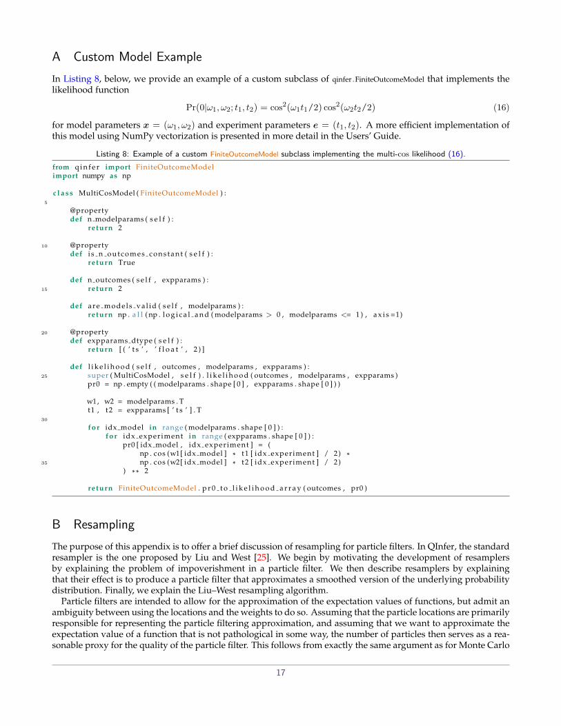
A Custom Model ExampleIn Listing 8, below, we provide an example of a custom subclass of qinfer .FiniteOutcomeModel that implements thelikelihood function

Pr(0|ω1,ω2; t1, t2) = cos2(ω1t1/2) cos2(ω2t2/2) (16)

for model parameters x = (ω1,ω2) and experiment parameters e = (t1, t2). A more efficient implementation ofthis model using NumPy vectorization is presented in more detail in the Users’ Guide.

Listing 8: Example of a custom FiniteOutcomeModel subclass implementing the multi-cos likelihood (16).from q i n f e r import FiniteOutcomeModelimport numpy as np

c l a s s MultiCosModel ( FiniteOutcomeModel ) :5

@propertydef n modelparams ( s e l f ) :

return 2

10 @propertydef i s n outcomes cons tant ( s e l f ) :

return True

def n outcomes ( s e l f , expparams ) :15 return 2

def are models va l id ( s e l f , modelparams ) :return np . a l l ( np . l o g i c a l a n d ( modelparams > 0 , modelparams <= 1 ) , a x i s =1)

20 @propertydef expparams dtype ( s e l f ) :

return [ ( ’ t s ’ , ’ f l o a t ’ , 2 ) ]

def l i k e l i h o o d ( s e l f , outcomes , modelparams , expparams ) :25 super ( MultiCosModel , s e l f ) . l i k e l i h o o d ( outcomes , modelparams , expparams )

pr0 = np . empty ( ( modelparams . shape [ 0 ] , expparams . shape [ 0 ] ) )

w1, w2 = modelparams . Tt1 , t2 = expparams [ ’ t s ’ ] . T

30

for idx model in range ( modelparams . shape [ 0 ] ) :for idx experiment in range ( expparams . shape [ 0 ] ) :

pr0 [ idx model , idx experiment ] = (np . cos (w1[ idx model ] * t1 [ idx experiment ] / 2) *

35 np . cos (w2[ idx model ] * t2 [ idx experiment ] / 2)) * * 2

return FiniteOutcomeModel . p r 0 t o l i k e l i h o o d a r r a y ( outcomes , pr0 )

B ResamplingThe purpose of this appendix is to offer a brief discussion of resampling for particle filters. In QInfer, the standardresampler is the one proposed by Liu and West [25]. We begin by motivating the development of resamplersby explaining the problem of impoverishment in a particle filter. We then describe resamplers by explainingthat their effect is to produce a particle filter that approximates a smoothed version of the underlying probabilitydistribution. Finally, we explain the Liu–West resampling algorithm.

Particle filters are intended to allow for the approximation of the expectation values of functions, but admit anambiguity between using the locations and the weights to do so. Assuming that the particle locations are primarilyresponsible for representing the particle filtering approximation, and assuming that we want to approximate theexpectation value of a function that is not pathological in some way, the number of particles then serves as a rea-sonable proxy for the quality of the particle filter. This follows from exactly the same argument as for Monte Carlo

17

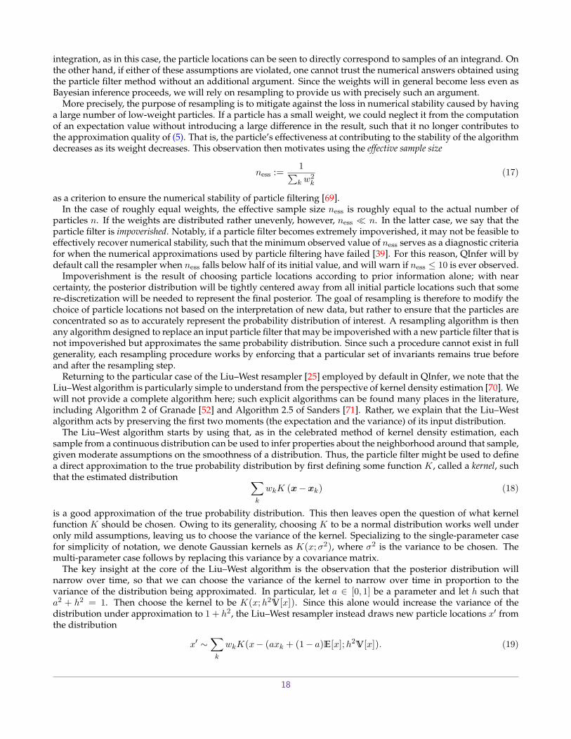
integration, as in this case, the particle locations can be seen to directly correspond to samples of an integrand. Onthe other hand, if either of these assumptions are violated, one cannot trust the numerical answers obtained usingthe particle filter method without an additional argument. Since the weights will in general become less even asBayesian inference proceeds, we will rely on resampling to provide us with precisely such an argument.

More precisely, the purpose of resampling is to mitigate against the loss in numerical stability caused by havinga large number of low-weight particles. If a particle has a small weight, we could neglect it from the computationof an expectation value without introducing a large difference in the result, such that it no longer contributes tothe approximation quality of (5). That is, the particle’s effectiveness at contributing to the stability of the algorithmdecreases as its weight decreases. This observation then motivates using the effective sample size

ness :=1∑k w

2k

(17)

as a criterion to ensure the numerical stability of particle filtering [69].In the case of roughly equal weights, the effective sample size ness is roughly equal to the actual number of

particles n. If the weights are distributed rather unevenly, however, ness � n. In the latter case, we say that theparticle filter is impoverished. Notably, if a particle filter becomes extremely impoverished, it may not be feasible toeffectively recover numerical stability, such that the minimum observed value of ness serves as a diagnostic criteriafor when the numerical approximations used by particle filtering have failed [39]. For this reason, QInfer will bydefault call the resampler when ness falls below half of its initial value, and will warn if ness ≤ 10 is ever observed.

Impoverishment is the result of choosing particle locations according to prior information alone; with nearcertainty, the posterior distribution will be tightly centered away from all initial particle locations such that somere-discretization will be needed to represent the final posterior. The goal of resampling is therefore to modify thechoice of particle locations not based on the interpretation of new data, but rather to ensure that the particles areconcentrated so as to accurately represent the probability distribution of interest. A resampling algorithm is thenany algorithm designed to replace an input particle filter that may be impoverished with a new particle filter that isnot impoverished but approximates the same probability distribution. Since such a procedure cannot exist in fullgenerality, each resampling procedure works by enforcing that a particular set of invariants remains true beforeand after the resampling step.

Returning to the particular case of the Liu–West resampler [25] employed by default in QInfer, we note that theLiu–West algorithm is particularly simple to understand from the perspective of kernel density estimation [70]. Wewill not provide a complete algorithm here; such explicit algorithms can be found many places in the literature,including Algorithm 2 of Granade [52] and Algorithm 2.5 of Sanders [71]. Rather, we explain that the Liu–Westalgorithm acts by preserving the first two moments (the expectation and the variance) of its input distribution.

The Liu–West algorithm starts by using that, as in the celebrated method of kernel density estimation, eachsample from a continuous distribution can be used to infer properties about the neighborhood around that sample,given moderate assumptions on the smoothness of a distribution. Thus, the particle filter might be used to definea direct approximation to the true probability distribution by first defining some function K, called a kernel, suchthat the estimated distribution ∑

k

wkK (x−xk) (18)

is a good approximation of the true probability distribution. This then leaves open the question of what kernelfunction K should be chosen. Owing to its generality, choosing K to be a normal distribution works well underonly mild assumptions, leaving us to choose the variance of the kernel. Specializing to the single-parameter casefor simplicity of notation, we denote Gaussian kernels as K(x;σ2), where σ2 is the variance to be chosen. Themulti-parameter case follows by replacing this variance by a covariance matrix.

The key insight at the core of the Liu–West algorithm is the observation that the posterior distribution willnarrow over time, so that we can choose the variance of the kernel to narrow over time in proportion to thevariance of the distribution being approximated. In particular, let a ∈ [0, 1] be a parameter and let h such thata2 + h2 = 1. Then choose the kernel to be K(x;h2V[x]). Since this alone would increase the variance of thedistribution under approximation to 1 + h2, the Liu–West resampler instead draws new particle locations x′ fromthe distribution

x′ ∼∑k

wkK(x− (axk + (1− a)E[x];h2V[x]). (19)

18

This distribution contracts each original particle towards the mean by 1− a, such that the mean and variance ofthe post-resampling distribution are identical to the distribution being approximated.

Importantly, the Liu–West generalizes existing resampling algorithms, such that the bootstrap [21] and assumeddensity filtering resamplers [53, 72] are given by a = 1 and a = 0, respectively. We also note that violating theinvariant that V[x] is preserved can allow for some robustness to multimodal distributions and time-dependence[52]. Finally, a video of the Liu–West resampler applied to Bayesian inference on the model of Listing 8 is availableonline [73].

19