qcd resummation techniques - arxiv.org · and, instead, it must be resummed. the development of...
TRANSCRIPT

arX
iv:h
ep-p
h/04
0302
3v1
2 M
ar 2
004
QCD Resummation Techniques
A Dissertation, Presented
by
Tibor Kucs
to
The Graduate School
in Partial Fulfillment of the
Requirements
for the Degree of
Doctor of Philosophy
in
Physics
State University of New York
at Stony Brook
May 2004
Dissertation Director: Prof. George Sterman

State University of New York
at Stony Brook
The Graduate School
Tibor Kucs
We, the dissertation committee for the above candidate for the Doctor ofPhilosophy degree, hereby recommend acceptance of this dissertation.
George StermanProfessor, C.N. Yang Institute for Theoretical Physics, SBU
Dissertation Director
Jack SmithChair, C.N. Yang Institute for Theoretical Physics, SBU
Chairman of Dissertation
Michael RijssenbeekProfessor, Department of Physics, SBU
Werner VogelsangDepartment of Physics, Brookhaven National Laboratory
Outside Member
This dissertation is accepted by the Graduate School.
Graduate School
ii

Abstract of the Dissertation
QCD Resummation Techniques
by
Tibor Kucs
Doctor of Philosophy
in
Physics
State University of New York
at Stony Brook
2004
Dissertation Director: Prof. George Sterman
The primary aim of high-energy QCD phenomenology is the de-
termination of cross sections for particle collisions. One of the
fundamental properties of QCD, the asymptotic freedom, suggests
that the coupling constant in this high-energy regime is small. Pro-
vided that the coefficients of the perturbative expansion are small
enough, the perturbation theory should give reliable results. How-
ever, in many quantities of interest the smallness of the expansion
coefficients is violated due to large logarithmic enhancements. In
this case the perturbation series cannot be truncated at fixed order
iii

and, instead, it must be resummed. The development of such re-
summation algorithms is the main subject of the research presented
in this thesis.
In the first part, we propose a resummation technique applicable
to the Regge limit, which is defined for elastic scattering as the
region of large energies and small momentum transfer. We develop
a new systematic procedure for this limit in perturbative QCD to
arbitrary logarithmic order. The formalism relies on the IR struc-
ture and the gauge symmetry of the theory. We identify leading
regions in loop momentum space responsible for the singular struc-
ture of the amplitudes and perform power counting to determine
the strength of these divergences. Using a factorization procedure
introduced by Sen, we derive a sum of convolutions in transverse
momentum space over soft and jet functions, which approximate
the amplitude up to power-suppressed corrections. A set of evolu-
tion equations generalizing the BFKL equation and controlling the
high energy behavior of the amplitudes to arbitrary logarithmic
accuracy is derived. The general method is illustrated in the case
of leading and next-to-leading logarithmic gluon reggeization and
BFKL equation. We confirm the standard results at LL accuracy.
At NLL order, we find an agreement with the reggeization conjec-
ture up to two loops. However, starting at three loop order, we
identify contributions violating the Regge ansatz. In addition, we
calculate the evolution kernel determining the high-energy behav-
iv
ior of the non-reggeized term in the scattering amplitude.
In the second part, we focus our attention to another intriguing
problem of high-energy QCD, the resummation associated with soft
radiation in dijet events which is complicated by the presence of
non-global logarithms. We introduce a set of correlations between
energy flow and event shapes that are sensitive to the flow of color
at short distances in jet events. These correlations are formulated
for a general set of event shapes, which includes jet broadening and
thrust as special cases. We illustrate the method for e+e− dijet
events, and calculate the correlation at leading logarithm in the
energy flow and at next-to-leading-logarithm in the event shape.
v

Contents
Acknowledgements x
1 Introduction 1
I Regge Resummation 6
2 The Method 7
2.1 Introduction . . . . . . . . . . . . . . . . . . . . . . . . . . . . 7
2.2 Kinematics and Gauge . . . . . . . . . . . . . . . . . . . . . . 11
2.3 Leading Regions, Power Counting . . . . . . . . . . . . . . . . 15
2.3.1 Singular contributions and reduced diagrams . . . . . . 15
2.3.2 Power counting . . . . . . . . . . . . . . . . . . . . . . 18
2.3.3 First factorized form . . . . . . . . . . . . . . . . . . . 25
2.4 The Jet Functions . . . . . . . . . . . . . . . . . . . . . . . . . 28
2.4.1 Decoupling of a soft gluon from a jet . . . . . . . . . . 28
2.4.2 Variation of a jet function with respect to a gauge fixing
vector η . . . . . . . . . . . . . . . . . . . . . . . . . . 31
vi

2.4.3 Dependence of a jet function on the plus component of
a soft gluon’s momentum attached to it . . . . . . . . . 34
2.5 Factorization and Evolution Equations . . . . . . . . . . . . . 36
2.5.1 Second factorized form . . . . . . . . . . . . . . . . . . 37
2.5.2 Evolution equation . . . . . . . . . . . . . . . . . . . . 41
2.5.3 Counting the number of logarithms . . . . . . . . . . . 47
2.5.4 Solution of the evolution equations . . . . . . . . . . . 49
2.6 Conclusions . . . . . . . . . . . . . . . . . . . . . . . . . . . . 54
3 The Applications 55
3.1 Amplitude at LL . . . . . . . . . . . . . . . . . . . . . . . . . 56
3.2 Amplitude at NLL . . . . . . . . . . . . . . . . . . . . . . . . 62
3.2.1 Evolution of Γ(n) at LL . . . . . . . . . . . . . . . . . . 74
3.3 Gluon reggeization at NLL . . . . . . . . . . . . . . . . . . . . 76
3.3.1 Color octet and negative signature amplitude . . . . . 76
3.3.2 NLL evolution equation for J(1)A . . . . . . . . . . . . . 80
3.4 Conclusions . . . . . . . . . . . . . . . . . . . . . . . . . . . . 85
II Resummation in Dijet Events 87
4 Event Shape / Energy Flow Correlations 88
4.1 Introduction . . . . . . . . . . . . . . . . . . . . . . . . . . . . 88
4.2 Shape/Flow Correlations . . . . . . . . . . . . . . . . . . . . . 93
4.2.1 Weights and energy flow in dijet events . . . . . . . . . 93
4.2.2 Weight functions and jet shapes . . . . . . . . . . . . . 97
4.2.3 Low order example . . . . . . . . . . . . . . . . . . . . 99
vii

4.3 Factorization of the Cross Section . . . . . . . . . . . . . . . . 103
4.3.1 Leading regions near the two-jet limit . . . . . . . . . . 104
4.3.2 The factorization in convolution form . . . . . . . . . . 107
4.3.3 The short-distance function . . . . . . . . . . . . . . . 112
4.3.4 The jet functions . . . . . . . . . . . . . . . . . . . . . 114
4.3.5 The soft function . . . . . . . . . . . . . . . . . . . . . 118
4.4 Resummation . . . . . . . . . . . . . . . . . . . . . . . . . . . 122
4.4.1 Energy flow . . . . . . . . . . . . . . . . . . . . . . . . 123
4.4.2 Event shape transform . . . . . . . . . . . . . . . . . . 126
4.4.3 The resummed correlation . . . . . . . . . . . . . . . . 130
4.4.4 The inclusive event shape . . . . . . . . . . . . . . . . 132
4.5 Results at NLL . . . . . . . . . . . . . . . . . . . . . . . . . . 133
4.5.1 Lowest order functions and anomalous dimensions . . . 133
4.5.2 Checking the ξc-dependence . . . . . . . . . . . . . . . 138
4.5.3 The inclusive event shape at NLL . . . . . . . . . . . . 139
4.5.4 Closed expressions . . . . . . . . . . . . . . . . . . . . 143
4.6 Numerical Results . . . . . . . . . . . . . . . . . . . . . . . . . 145
4.7 Summary and Outlook . . . . . . . . . . . . . . . . . . . . . . 148
A 151
A.1 Power counting with contracted vertices . . . . . . . . . . . . 151
A.2 Varying the Gauge-Fixing Vector . . . . . . . . . . . . . . . . 157
A.3 Tulip-Garden Formalism . . . . . . . . . . . . . . . . . . . . . 161
A.4 Feynman Rules . . . . . . . . . . . . . . . . . . . . . . . . . . 163
A.5 Origin of Glauber Region . . . . . . . . . . . . . . . . . . . . . 165
viii
B 167
B.1 Symmetry property of the jet functions . . . . . . . . . . . . . 167
B.2 Evolution kernel . . . . . . . . . . . . . . . . . . . . . . . . . . 170
C 184
C.1 Eikonal Example . . . . . . . . . . . . . . . . . . . . . . . . . 184
C.2 Recoil . . . . . . . . . . . . . . . . . . . . . . . . . . . . . . . 188
Bibliography 204
ix

Acknowledgements
It is my pleasure to thank all the people who directly or indirectly influenced
the course of my research and without whom this work would have never been
completed.
I wish to thank my adviser George Sterman for his patient guidance and
invaluable help during my graduate career. I would also like to thank my
collaborators Carola F. Berger and Maarten Boonekamp for working with me
on many challenging problems. I am grateful to Zurab Kakushadze, Peter
van Nieuwenhuizen, Martin Rocek, Robert Shrock, Jack Smith and George
Sterman for wonderful lectures on quantum field theory, particle physics and
string theory that I was lucky to attend. I am very thankful to Michael
Rijssenbeek and Werner Vogelsang for making it possible to spend very fruitful
research periods at CERN and BNL, respectively. My first steps in particle
physics started in Prague, where Jiri Formanek, Jiri Horejsi and Jiri Chyla had
very positive influence on me. I have also benefited from many physics and
non-physics related conversations with my friends Lilia Anguelova, Nathan
Clisby, Olindo Corradini, Alberto Iglesias, Peter Langfelder, Valer Zetocha
and Kostas Zoubos during the years spent at Stony Brook.
Last but definitely not least, I am indebted to my parents and to my wife

Simona for their love and overall support during my educational period.
Chapter 1
Introduction
The birth of modern theory of strong interactions dates back to the early
sixties when Gell-Mann and Zweig, [1] proposed the quark model to describe
the properties of hadrons. This model suggests that all strongly interacting
objects are composed of more elementary constituents named quarks. The
first experimental support of this idea came in the late sixties at SLAC in
a Deeply Inelastic Scattering. After this, the top priority became the hunt
for a theory describing the dynamics of quarks. The distinctive feature of
quarks is that they carry internal quantum number called color. Each quark
can be in three color states. In the early seventies, Fritzsch, Gell-Mann and
Leutwyler, Ref. [2], proposed a gauge theory describing the interaction between
these quarks, called Quantum Chromodynamcis (QCD). The mediator of this
interaction, analogous to a photon in QED, is a gluon. At the classical level,
QCD is invariant under the color SU(3) local gauge transformations. The
quarks transform in the fundamental representation and the gluons in the
adjoint representation of this group. The process of quantization introduces
1

a gauge-fixing and the ghost terms into the Lagrangian. It satisfies a global
residual gauge symmetry, called BRS symmetry, Ref. [3]. This symmetry
proves to be very powerful in deriving identities between Green functions which
are exact, i.e. they hold to all orders in perturbation theory.
The use of QCD as a perturbation theory is justified due to the property
of asymptotic freedom discovered by ’t Hooft, Gross, Wilczek and Politzer [4].
This property says that with increasing energies the coupling characterizing
the interaction between the quarks and gluons decreases.
At the Ultra-Violet (UV) spectrum of internal momenta, the 4-D field the-
ory is plagued by infinities. They appear since the current theory is only an
effective theory valid in a certain energy regime. At sufficiently high energies it
must, presumably, be embedded into some more fundamental theory. Never-
theless the theory is internally consistent, since we can remove these infinities
by the process of renormalization, [5].
On the opposite end of momentum spectra, we encounter another type of
divergences due to the Infra-Red (IR) region of soft momenta and collinear
momenta. These divergences occur only for Green functions with external
particles on-shell, when at least one of the particles is massless. Their origin
is due to the degeneracy of states occurring in the soft and collinear limit,
since we cannot possibly distinguish soft emissions and collinear splittings from
situations when these emissions and splittings are absent. This observation
suggests, that although IR divergences appear on a diagram by diagram basis,
they cancel in properly averaged quantities. Namely, one needs to sum over
all indistinguishable states. Already in 1937, Bloch and Nordsieck, Ref. [6],
showed that this is, indeed, the case in QED when the summation over final
2
states is performed.
In QCD the situation is more complicated due to the self-coupling of gluons.
In this case the KLN theorem, Ref. [7], which extends the summation over
final state degeneracies to initial states as well, comes to our rescue. It is these
quantities, which are free of IR divergences in QCD. From the experimental
point of view this solution to the IR problem has a caveat, however. We can
hardly expect to prepare our initial states in collision experiments to satisfy the
conditions of the KLN theorem. Instead, we take one step further and invoke
factorization theorems, Ref. [8]. It is exactly these theorems that enable us to
turn perturbative QCD to a predictive calculational tool.
Factorization theorems claim that it is possible to separate short and long
distance physics in physical quantities. A cross section for hadronic colli-
sion can be written as a convolution over functions describing long distance
dynamics, which can be either Parton Distribution Functions (PDFs) or Frag-
mentation Functions (FFs), and functions describing short distance physics,
which are partonic cross sections. The former have a physical interpretation of
probabilities to find partons inside hadrons in case of PDFs, or to find hadrons
inside partons in the case of FFs. These quantities cannot be completely de-
termined from perturbative QCD and need to be fitted to experimental data.
However, perturbative QCD enables us to find the evolution of the density
functions with energy scale, Ref. [9]. These evolution equations resum large
logarithmic corrections in this energy scale. They are the consequence of the
factorized form for the cross section and the renormalization group equation
stating that the physical quantities cannot depend on the scale at which we
make the separation of short and long distance dynamics. Actually, under
3

very general assumptions, we can claim that whenever there is a factorization,
there is a corresponding resummation. We will encounter concrete examples
of this statement in later chapters. The main feature of the distribution func-
tions is that they are process independent. This suggests that after fitting long
distance functions in one process, we can use them in certain other processes
involving the same type of hadron.
The second ingredient of the factorized cross section is the partonic cross
section, which quantifies the interaction of the underlying partons in the hard
process. This quantity is IR safe and calculable within perturbation theory
provided the coefficients of the perturbative expansion are small. This is, how-
ever, not always the case. The coefficients are usually enhanced at kinematic
edges of phase space. The reason for this is easily understood. The cancellation
of IR divergences happens between virtual and real corrections. The integra-
tion in the virtual corrections spans all the energy scales: soft, hard and UV.
The last one is removed by renormalization, so only the region between the soft
and the hard scale remains. The phase space for real corrections depends on
the kinematics considered. If we are completely inclusive then the integration
region is the same as in the case of virtual corrections and there is a perfect
cancellation between the two. However, once we impose kinematic constraints
on the final state, then the cancellation between the two is incomplete and we
can be left with large logarithms spoiling the perturbative expansion. In this
case we need to resum the perturbation series.
The development of resummation procedures for various processes is the
main topic of this work. It consists of two parts. In the first part we propose
a systematic resummation technique applicable in the Regge limit, Ref. [10]
4

- [11]. This limit concerns almost forward elastic scattering of particles. In
the second part of this thesis we pursue resummation of soft radiation accom-
panying final state jets in lepton collisions, Ref. [12].
5

Part I
Regge Resummation
6

Chapter 2
The Method
2.1 Introduction
The study of semi-hard processes within the framework of gauge quantum
field theories has a long history. For reviews see Refs. [13]- [15]. The defin-
ing feature of such processes is that they involve two or more hard scales,
compared to ΛQCD, which are strongly ordered relative to each other. The
perturbative expansions of scattering amplitudes for these processes must be
resummed since they contain logarithmic enhancements due to large ratios of
the scales involved. One of the most important examples is elastic 2 → 2
particle scattering in the Regge limit, s ≫ |t| (with s and t the usual Mandel-
stam variables). It is this process that we investigate in the next two chapters.
We extend the techniques developed in Refs. [16] and [17] and devise a new
systematic method for evaluation of QCD scattering amplitudes in the Regge
limit to arbitrary logarithmic accuracy, Ref. [10].
The problem of the Regge limit in quantum field theory was first tackled in
7

the case of fermion exchange amplitude within QED in Ref. [18]. Here it was
found that the positive signature amplitude takes a reggeized form up to the
two loop level in Leading Logarithmic (LL) approximation. In Ref. [19] the
calculations were extended to higher loops, and the imaginary part of the Next-
to-Leading Logarithms (NLL) was also obtained. The analysis in Refs. [18]
and [19] was performed in Feynman gauge. It was realized in Ref. [20] that a
suitable choice of gauge can simplify the class of diagrams contributing at LL.
The common feature of all this work was the use of fixed order calculations.
To verify that the pattern of low order calculations survives at higher orders, a
method to demonstrate the Regge behavior of amplitudes to all orders is nec-
essary. This analysis was provided by A. Sen in Ref. [16], in massive QED. Sen
developed a systematic way to control the high energy behavior of fermion and
photon exchange amplitudes to arbitrary logarithmic accuracy. The formalism
relies heavily on the IR structure and gauge invariance of QED and provides
a proof of the reggeization of a fermion at NLL to all orders in perturbation
theory.
The resummation of color singlet exchange amplitudes in non-abelian gauge
theories in LL was achieved in the pioneering work of Ref. [21], where the
reggeization of a gluon in LL was also demonstrated. The evolution equations
resumming LL in the case of three gluon exchange was derived in Ref. [22]. In
Ref. [17], n-gluon exchange amplitudes in QCD at LL level were studied and a
set of evolution equations governing the high energy behavior of these ampli-
tudes was obtained at LL. A different approach was undertaken in Ref. [23].
Here n → m amplitudes were studied in SU(2) Higgs model with spontaneous
symmetry breaking. Starting with the tree level amplitudes, an iterative proce-
8

dure was developed, which generates a minimal set of terms in the perturbative
expansion that have to be taken into account in order to satisfy the unitarity
requirement of the theory. See also Ref. [24]. The extension of the BFKL
formalism to NLL spanned over a decade. For a review see Ref. [25]. The
building blocks of NLL BFKL are the emissions of two gluons or two quarks
along the ladder, Ref. [26], one loop corrections to the emission of a gluon along
the ladder, Ref. [27], and the two loop gluon trajectory, Refs. [28], [29], [30]
and [31]. The particular results were put together in Ref. [32]. In Ref. [33],
the trajectory for the fermion at NLL was evaluated by taking the Regge limit
of the explicit two loop partonic amplitudes, Ref. [34].
Besides the NLO perturbative corrections to the BFKL kernel a variety
of approaches have been developed for unitarization corrections, Refs. [35–
37], which extend the BFKL formalism by incorporating selected higher-order
corrections. The procedure proposed in this work, Refs. [10] and [11], in a
way, places these approaches in an even more general context. In principle,
it makes it possible to find the scattering amplitudes to arbitrary logarithmic
accuracy and to determine the evolution kernels to arbitrary fixed order in the
coupling constant. The formalism contains all color structures and, of course,
the construction of the amplitude to any given level requires the computation
of the kernels and the solution of the relevant equations.
The first part of the thesis is organized as follows. In Chapter 2, we develop
the general algorithm. In Sec. 2.2 we discuss the kinematics of the partonic
process under study and the gauge used. In Sec. 2.3 we identify the leading
regions in internal momentum space, which produce logarithmic enhancements
in the perturbation series. After identifying these regions, we perform power
9

counting to verify that the singularity structure of individual diagrams is at
worst logarithmic. The leading regions lead to a factorized form for the ampli-
tude (First Factorized Form). It consists of soft and jet functions, convoluted
over soft loop momenta, which can still produce logarithms of s/|t|. In Sec.
2.4 we study the properties of the jet functions appearing in the factorization
formula for the amplitude. We show how the soft gluons can be factored from
the jet functions. In Sec. 2.5 we demonstrate how to express systematically the
amplitude as a convolution in transverse momenta. In this form all the large
logarithms are organized in jet functions and the soft transverse momenta in-
tegrals do not introduce any logarithms of s/|t| (Second Factorized Form). We
derive evolution equations that enable us to control the high energy behavior
of the scattering amplitudes.
In Chapter 3, we illustrate the general method valid to all logarithmic
accuracy in the case of LL and NLL in the amplitude and we examine the
evolution equations at the same level. In Sec. 3.1, we resum the amplitude at
LL and we find the LL gluon Regge trajectory. In Sec. 3.2, we analyze the
amplitude at NLL order. We confirm the LL BFKL evolution equation. In
Sec. 3.3, we address the problem of NLL evolution equations and the gluon
reggeization at this accuracy. We confirm the Regge hypothesis at two loop
level. However, we identify contributions violating the Regge ansatz starting
at three loop order.
Some technical details are discussed in appendices A.1 - B.2. The first
appendix treats power counting for regions of integration space where internal
loop momenta become much larger than the momentum transfer. In Appendix
A.2 we illustrate the origin of special vertices encountered due to the resum-
10

mation. In Appendix A.3 we show a systematic expansion for the amplitude
leading to the first factorized form. In Appendix A.4 we list the Feynman
rules used throughout the text. In Appendix A.5 we demonstrate the origin
of extra soft momenta configurations (Glauber region) which need to be con-
sidered in the analysis of amplitudes in the Regge limit. In Appendix B.1, we
study some symmetry properties of jet functions and finally in Appendix B.2,
we give details on the derivation of the color octet NLL evolution equations.
2.2 Kinematics and Gauge
We analyze the amplitude for the elastic scattering of massless quarks
q(pA, rA, λA) + q′(pB, rB, λB) → q(pA − q, r1, λ1) + q′(pB + q, r2, λ2), (2.1)
within the framework of perturbative QCD in the kinematic region s ≫ −t
(Regge limit), where s = (pA +pB)2 and t = q2 are the usual Mandelstam vari-
ables. We stress, however, that the results obtained below apply to arbitrary
elastic two-to-two partonic process. We pick process (2.1) for concreteness
only. The arguments in Eq. (2.1) label the momenta, pi, the colors, ri, and
polarizations, λi, for i = A, B, 1, 2, respectively, of the initial and final state
quarks. We choose to work in the center-of-mass (c.m.) where the momenta
of the incoming quarks and the momentum transfer have the following com-
11

ponents 1
pA =
(√
s
2, 0−, 0⊥
)
,
pB =
(
0+,
√
s
2, 0⊥
)
,
q = (0+, 0−, q⊥). (2.2)
Strictly speaking q± = ±|t|/√
2s, so the q± components vanish in the Regge
limit only.
In the color basis
b1 = δrA, r1δrB , r2 ,
b8 = − 1
2Nc
δrA, r1δrB , r2 +1
2δrA, r2δrB, r1, (2.3)
with Nc the number of colors, we can view the amplitude for process (2.1) as
a two dimensional vector in color space
A =
A1
A8
, (2.4)
where A1 and A8 are defined by the expansion
A rA rB, r1 r2 = A1 (b1)rA rB , r1 r2 + A8 (b8)rA rB , r1 r2 . (2.5)
Since the amplitude is dimensionless and all particles are massless, its compo-
1We use light-cone coordinates, v = (v+, v−, v⊥), v± = (v0 ± v3)/√
2.
12
nents can depend, in general, on the following variables
Ai ≡ Ai
(
s
µ2,
t
µ2, αs(µ
2), ǫ
)
for i = 1, 8, (2.6)
where µ is a scale introduced by regularization. We use dimensional regu-
larization in order to regulate both infrared (IR) and ultraviolet (UV) di-
vergences with D = 4 − 2ε the number of dimensions. Choosing the scale
µ2 = s, the strong coupling, αs(µ), is small. However, in general, an in-
dividual Feynman diagram contributing to the process (2.1) at r-loop order
can give a contribution as singular as (s/t) αr+1s ln2r(−s/t). In Sec. 2.5.3 we
will confirm that there is a cancellation of all terms proportional to the i-th
logarithmic power for i = r + 1, . . . , 2r at order αr+1s in the perturbative ex-
pansion of the amplitude. Hence at r loops the amplitude is enhanced by a
factor (s/t) αr+1s lnr(−s/t), at most. In order to get reliable results in pertur-
bation theory we must, nevertheless, resum these large contributions. In the
k-th non-leading logarithmic approximation one needs to resum all the terms
proportional to (s/t) αr+1s lnr−j(−s/t), j = 0, . . . , k at r-loop level.
We perform our analysis in the Coulomb gauge, where the propagator of a
gluon with momentum k has the form
−i δabNαβ(k, k)
k2 + iǫ≡ −i δab
1
k2 + iǫ
(
gαβ − kα kβ + kα kβ − kα kβ
k · k
)
, (2.7)
in terms of the vector
k = k − (k · η) η, (2.8)
13

with
η =
(
1√2,
1√2, 0⊥
)
, (2.9)
an auxiliary four-vector defined in the partonic c.m. frame. The numerator of
the gluon propagator satisfies the following identities
kα Nαβ(k, k) = k2 kβ − kβ
k · k ,
kα Nαβ(k, k) = 0. (2.10)
The first equality in Eq. (2.10) is the statement that the nonphysical degrees of
freedom do not propagate in this gauge. For use below, we list the components
of the gluon propagator:
N+−(k) = N−+(k) =k+k− − k2
⊥k · k ,
N++(k) = N−−(k) =k+k−
k · k ,
N± i(k) = N i ±(k) = ±(k− − k+)ki
2k · k ,
N i j(k) = N j i(k) = gij − kikj
k · k . (2.11)
We note that these are symmetric functions under the transformation k± →
−k±, except for the components N± i = N i ±, which are antisymmetric under
this transformation. It was demonstrated in Ref. [38] that QCD is renormal-
izable in Coulomb gauge, by considering a class of gauges which interpolates
between the covariant (Landau) and the physical (Coulomb) gauge.
14

2.3 Leading Regions, Power Counting
In order to resum the Regge logarithms, we need to identify the regions of
integration in the loop momentum space that give rise to singularities in the
limit t/s → 0. We follow the method developed in Refs. [39,40], which begins
with the identification of the relevant regions in momentum space.
2.3.1 Singular contributions and reduced diagrams
The singular contributions of a Feynman integral come from the points in loop
momentum space where the integrand becomes singular due to the vanishing
of propagator denominators. However, in order to give a true singularity the
integration variables must be trapped at such a singular point. Otherwise we
can deform the integration contour away from the dangerous region. These
singular points are called pinch singular points. They can be identified with
the following regions of integration in momentum space,
1. soft momenta, with scaling behavior kµ ∼ σ√
s for all components
(σ ≪ 1),
2. momenta collinear to the momenta of the external particles, with scaling
behavior
k+ ∼ √s, k− ∼ λ
√s, |k⊥| ∼ λ1/2
√s for the particles moving in the +
direction and
k+ ∼ λ√
s, k− ∼ √s, |k⊥| ∼ λ1/2
√s for the particles moving in the −
direction,
3. so-called Glauber or Coulomb momenta, Ref. [41], with scaling behavior
15

ABS0 = A
BS0S ABS0a) b) )
Figure 2.1: The reduced diagrams a) and c) contributing to the amplitude.Diagram b) represents a decomposition of diagram a) for the purpose of powercounting.
k± ∼ σ± √s, |k⊥| ∼ σ
√s, where λ . σ± . σ, and where the scaling
factors λ, σ satisfy the strong ordering λ ≪ σ ≪ 1 (The origin of this
region is illustrated in Appendix A.5.),
4. hard momenta, having the scaling behavior kµ ∼ √s for all components.
The extra gauge denominators 1/(k · k) originating from the numerators of
the gluon propagator, Eq. (2.7), do not alter the classification of the pinch
singular points mentioned above. Actually, only the subsets 1 and 3 in the
above classification can be produced due to the extra gauge denominators.
With every pinch singular point, we may associate a reduced diagram,
which is obtained from the original diagram by contracting all hard lines (sub-
set 4) at the particular singular point. As shown in Refs. [39, 40, 42] the
reduced diagram corresponding to a given pinch singular point must describe
a real physical process, with each vertex of the reduced diagram representing
a real space-time point. This physical interpretation suggests two types of
reduced diagrams contributing to the process (2.1), shown in Fig. 2.1.
16

The jet A(B) contains lines whose momenta represent motion in the + (−)
direction. The lines included in the blob S ′ and the lines coming out of it are
all soft (configurations 1 and 3 in the classification of loop momenta described
above). These two oppositely moving (virtual) jets may interact through the
exchange of soft lines, Fig. 2.1a, and/or they can meet at one or more space-
time points, Fig. 2.1c.
Having found the most general reduced diagrams giving the leading be-
havior of the amplitude for process (2.1) in the Regge limit, we can estimate
the strength of the IR divergence of the integral near a given pinch singular
point. First we restrict ourselves to cases involving subsets 1 and 2 from the
classification of loop momenta above. To do so, we count powers in the scaling
variables λ and σ.
The scaling behavior of these loop momenta implies that every soft loop
momentum contributes a factor σ4, every jet loop momentum gives rise to
the power λ2, every internal soft boson (fermion) line provides a contribu-
tion σ−2 (σ−1) and every internal jet line (fermionic or bosonic) scales as λ−1.
In addition, there can be suppression factors arising from the numerators of
the propagators associated with internal lines and from internal vertices. As
pointed out in Ref. [39], in physical gauges each three-point vertex connecting
three jet lines is associated with a numerator factor that vanishes at least lin-
early in the components of the transverse jet momenta, and therefore provides
a suppression λ1/2.
We are now ready to estimate the power of divergence corresponding to
the reduced diagrams describing our process. First we restrict ourselves to
the case shown in Fig. 2.1a. As indicated schematically in Fig. 2.1b, we can
17

perform the power counting for the jets and for the soft part separately. All
soft propagators and all soft loop momenta are included in the soft subdiagram
S. The superficial degree of IR divergence of the reduced diagram R from Fig.
2.1a and Fig. 2.1b can then be written as
ω(R) = ω(A) + ω(B) + ω(S), (2.12)
where the external lines and loops of S ′ are included in S. For ω(R) > 0
the overall integral is finite, while ω(R) ≤ 0 corresponds to an IR divergent
integral. When ω(R) = 0, the integral diverges logarithmically. Here we set
λ ∼ σ for power counting purposes. We come back to the effect of relaxing
this condition in connection with a discussion of item 3, Glauber regions, in
our list of singular momentum configurations.
2.3.2 Power counting
In this subsection, we consider the case when all vertices in a diagram are
elementary only, that is, without contracted sub-diagrams carrying large loop
momenta. In Appendix A.1 we show that our conclusions are unchanged by
contracted vertices.
We perform the power counting for the soft part S first. Let f, b be the
number of fermion, boson lines external to S′
and let E = f+b. The superficial
degree of divergence for S, found by summing powers of σ, can be written
ω(S) = 4(E − 2) − 2b − f + 2 + ω(S′
), (2.13)
18

where the first term is due to loop integrations linking S ′ to the jets, while
the second and the third terms originate from propagators associated with
the bosonic and fermionic lines, respectively, connecting the jets A, B and
the soft part S ′. The term +2 is introduced because we are resumming only
leading power corrections proportional to s/t and therefore we exclude the
overall factor s/t from the power counting. Since the lines entering S ′ are soft,
we obtain the superficial degree of divergence for S ′ simply from dimensional
analysis. It is given by
ω(S′
) = 4 − b − 3f/2. (2.14)
Combining Eqs. (2.13) and (2.14), the superficial degree of infrared divergence
for the soft part S is then
ω(S) = b + 3f/2 − 2. (2.15)
Before carrying out the jet power counting, we introduce some notation.
Let EA be the number of soft lines attached to jet A; I is the total number
of jet internal lines; vα is the number of α-point vertices connecting jet lines
only; wα has a meaning similar to vα, with the difference that every vertex
counted by wα has at least one soft line attached to it. These are the vertices
that connect the jet A to the soft part S. Finally, L denotes the number of
loops internal to jet A. As noted above, we will perform the power counting
for the case when the scaling factor for the soft momenta, σ, is of the same
order as the scaling factor for jet A momenta. When the scaling factors are
19

different we encounter subdivergencies, which can be analyzed the same way
as described below. We also assume that there are no internal and external
ghost lines included in the jet function. Later we will discuss the effect of
adding ghost lines.
The superficial degree of divergence for jet A can now be expressed as
ω(A) = 2L − I + v3/2. (2.16)
The last term represents the suppression factor associated with the three point
vertices. We denote the total number of vertices internal to jet A by
v =∑
α
(vα + wα). (2.17)
Next we use the Euler identity relating the number of loops, internal lines and
vertices of jet A
L = I − v + 1, (2.18)
and the relation between the number of lines and the number of vertices
2I + EA + 2 =∑
α
α(vα + wα). (2.19)
Using Eqs. (2.16)-(2.19) we arrive at the following form for the superficial
degree of divergence for jet A
ω(A) = 1 − (EA + w3)/2 +∑
α≥5
(α − 4)(vα + wα)/2. (2.20)
20

Since every vertex counted by wα connects at least one external soft line, we
have the condition
EA ≥ w3 +∑
α≥4
wα. (2.21)
The equality holds when there is no vertex with two or more soft lines attached
to it. Combining Eqs. (2.20)-(2.21) we arrive at the following lower bound on
the superficial degree of divergence for jet A:
ω(A) ≥ 1 − EA +∑
α≥4
wα/2 +∑
α≥5
(α − 4)(vα + wα)/2. (2.22)
The third and the last term in Eq. (2.22) are always positive or zero and hence
ω(A) ≥ 1 − EA. (2.23)
A similar result holds for jet B, and therefore the superficial degree of collinear
divergence for jets A and B is
ω(A) + ω(B) ≥ 2 − E, (2.24)
with E = EA + EB as in Eq. (2.13). Combining the results for soft and jet
power counting, Eqs. (2.15) and (2.24), respectively in Eq. (2.12), we finally
obtain the superficial degree of IR divergence for the reduced diagram in Fig.
2.1a,
ω(R) ≥ f/2. (2.25)
This condition says that we can have at worst logarithmic divergences, pro-
vided no soft fermion lines are exchanged between the jets A and B. We
21

can therefore conclude that a reduced diagram from Fig. 2.1a containing ele-
mentary vertices can give at worst logarithmic enhancements in perturbation
theory. In order for the divergence to occur, the following set of conditions
must be satisfied:
1. There is an exchange of soft gluons between the jets A and B only, with
no soft fermion lines attached to the jets.
2. The jets A and B contain 3 and 4 point vertices only, see Eq. (2.22).
3. Soft gluons are connected to jets only through 3 point vertices, Eq.
(2.22), and at most one soft line is attached to each vertex inside the
jets, Eq. (2.21).
4. In the reasoning above we have assumed that there is no suppression
factor associated with the vertices where soft and jet lines meet. In
order for this to be true, the soft gluons must be connected to the jet
A(B) lines via the +(−) components of the vertices.
Next we consider adding ghost lines to the jet functions. As we review in
Appendix A.4, the propagator for a ghost line with momentum k is propor-
tional to 1/(k · k). Hence every internal ghost line belonging to the jet gives
a contribution which is power suppressed as 1/s. Since the numerator factors
do not compensate for this suppression, we can immediately conclude that the
jet functions cannot contain internal or external ghost lines at leading power.
So far we have not taken into account the possibility when the soft loop
momenta are pinched by the singularities of the jet lines. This situation allows
different components of soft momenta to scale differently. For example, a
22
minus component of soft momentum can scale as the minus component of jet
A momentum λ, while the rest of the soft momentum components may scale
as σ, where λ ≪ σ ≪ 1. The origin of these extra pinches is illustrated in
Appendix A.5.
Let us see what happens when we attach the ends of a gluon line with this
extra pinch to jet A at one end and the soft subdiagram S at the other end.
The integration volume for this soft loop momentum scales as λσ3. The soft
gluon denominator gives a factor σ−2. If this soft gluon is connected to the soft
part at a 4-point vertex, there is no new denominator in the soft part. On the
other hand, if the soft gluon is attached to the soft part via a 3-point vertex
then the extra denominator including the numerator suppression factors scales
as σ−1. The new jet line scales as λ−1 as long as the condition λ1/2 & σ is
obeyed; otherwise, we have the scaling σ−2 for the extra jet line. For λ1/2 & σ
the Glauber region produces logarithmic infrared divergence. When λ1/2 . σ,
the overall scaling factor λ/σ2 indicates power suppressed contribution.
Let us now investigate another possibility, when the soft gluon connects jet
A and jet B directly and its momentum is pinched by the singularities of the
jet A and the jet B lines. Denoting the scaling factors of jet A and jet B as λA
and λB, respectively, the integration volume provides the factor λAλBσ2 and
the soft gluon denominator contributes the power σ−2. The extra jet A and
jet B denominators scale as λ−1A and λ−1
B , provided λ1/2A & σ and λ
1/2B & σ. For
λ1/2A,B . σ both extra jet denominators provide the scaling factor σ−2. When
λ1/2A,B & σ, the power counting suggests logarithmically divergent integrals.
We have therefore verified that when the softest component of a soft line
satisfies the ordering σ2 . λ . σ, the Glauber (Coulomb) momenta produce
23

logarithmically IR divergent integrals and need to be taken into an account
when identifying enhancements in perturbation series. The analysis demon-
strated above for the case of one Glauber gluon can be extended to the situa-
tion with arbitrary number of Glauber gluons. This follows from dimensional
analysis, in a similar fashion as the treatment of purely soft loop momenta
above.
We conclude that the reduced diagram in Fig. 2.1a is at most logarithmi-
cally IR divergent, modulo the factor s/|t|. The reduced diagram in Fig. 2.1b
looses one small denominator compared to the reduced diagram in Fig. 2.1a
and since we are working in physical gauge, this loss cannot be compensated
by a large kinematical factor coming from the numerator. Hence the reduced
diagram in Fig. 2.1b is power suppressed compared to the reduced diagram in
Fig. 2.1a, and we do not need to consider it at leading power.
Finally, let us discuss the scale of the soft momenta. In the case of soft
exchange lines, each gluon propagator supplies a factor 1/(σ2 s), which we
want to keep at or below the order t in the leading power approximation.
Thus the size of the scale is fixed to be σ ∼√
|t|/√s. In the case of soft
lines which are attached to jet A or to jet B only, the scaling factor lies in the
interval (√
|t|/√s, 1). In the case of Glauber momenta, we again need σ ∼√
|t|/√s. Then the condition λ1/2 & σ, which is necessary for the logarithmic
enhancement, implies that the scaling factors for + and − components of the
Glauber (Coulomb) momenta can go down to |t|/s, the scale of the small
components of jet momenta. Additionally, we should note that soft and jet
sub-diagrams that do not carry the momentum transfer may approach the
mass shell (λ, σ → 0). Such lines produce true infrared divergences, which
24

Ak1a1 k2a2 knan B
p1b1 p2b2 pmbma) b)Figure 2.2: Jet A moving in the + direction (a) and jet B moving in the −direction (b).
we assume are made finite by dimensional regularization to preserve the gauge
properties that we will use below. The same power counting as above shows
that these divergences are also at worst logarithmic.
2.3.3 First factorized form
The analysis of the previous subsection suggests the following decomposition
of the leading reduced diagram from Fig. 2.1a. Let us denote the (n + 2)-
point and (m + 2)-point Green functions, 1PI in external soft gluon lines,
corresponding to jet A, J(n) a1... an
(A) µ1... µn(pA, q, η; k1, . . . , kn), Fig. 2.2a, and to jet B,
J(m) b1... bm
(B) ν1... νm(pB, q, η; p1, . . . , pm), Fig. 2.2b, respectively. The jet function J
(n)(A)
(J(m)(B) ) also depends on the color of the incoming and outgoing partons rA,
r1 (rB, r2), as well as on their polarizations λA, λ1 (λB, λ2), respectively. In
order to avoid making the notation even more cumbersome we do not exhibit
this dependence explicitly. In addition the dependence of J(n)(A) and J
(m)(B) on
the renormalization scale µ and the running coupling αs(µ) is understood.
The jet functions also depend on the following parameters: the gauge fixing
vector η, Eq. (2.9), of the Coulomb gauge, the four momenta of the external
25
soft gluons attached to jet A (B), k1, . . . , kn (p1, . . . , pm), and the Lorentz and
color indices of the soft gluons attached to the jet A (B), µ1, . . . , µn; a1, . . . , an
(ν1, . . . , νm; b1, . . . , bm). The momenta of the soft gluons attached to the jets
A and B satisfy the constraints∑n
i=1 ki = q and∑m
j=1 pj = q.
According to the results of the power counting, the soft gluons couple to jet
A via the minus components of their polarizations, and to jet B via the plus
components of their polarizations. Therefore, only the following components
survive in the leading power approximation
J(n) a1... an
A (pA, q, η, vB; k1, . . . , kn) ≡(
n∏
i=1
vµi
B
)
J(n) a1... an
(A) µ1... µn(pA, q, η; k1, . . . , kn),
J(m) b1... bm
B (pB, q, η, vA; p1, . . . , pm) ≡(
m∏
i=1
vνiA
)
J(m) b1... bm
(B) ν1... νm(pB, q, η; p1, . . . , pm),
(2.26)
where we have defined light-like momenta in the plus direction vA = (1, 0, 0⊥)
and in the minus direction vB = (0, 1, 0⊥). We can now write the contribution
to the reduced diagram in Fig. 2.1a, and hence to the amplitude for process
(2.1), in the form
A =∑
n,m
∫
(
n−1∏
i=1
dDki
)
∫
(
m−1∏
j=1
dDpj
)
J(n) a1... an
A (pA, q, η, vB; k1, . . . , kn)
× S(n,m)a1... an,b1... bm
(q, η, vA, vB; k1, . . . , kn; p1, . . . , pm)
× J(m) b1... bm
B (pB, q, η, vA; p1, . . . , pm), (2.27)
where the sum over repeated color indices is understood. Corrections to Eq.
(2.27) are suppressed by positive powers of t/s. The jet functions JA,B are de-
26

fined in Eq. (2.26) in the leading power accuracy. The internal loop momenta
of the jets A, B and of the soft function S are integrated over. The soft function
will, in general, include delta functions setting some of the momenta k1, . . . , kn
and color indices a1, . . . , an of jet function JA to the momenta p1, . . . , pm and
to the color indices b1, . . . , bm of jet function JB. The construction of the soft
function S is described in Appendix A.3. For a given Feynman diagram there
exist many reduced diagrams of the type shown in Fig. 2.1a, and one has to be
careful in systematically expanding this diagram into the terms that have the
form of Eq. (2.27). This systematic method can be achieved using the “tulip-
garden” formalism first introduced in Ref. [44] and used in a similar context
in Ref. [16]. For convenience of the reader we summarize this procedure in
Appendix A.3.
Let us now identify the potential sources of the enhancements in ln(s/|t|) of
the amplitude given by Eq. (2.27). If we integrate over the internal momenta of
the jet functions then we can get ln((pA · η)2/|t|) from JA and ln((pB · η)2/|t|)
from JB. In addition, according to the results of the power-counting, Eq.
(2.23), we know that the jet function with n external soft gluons diverges as
1/λn−1. After performing the integrals over the minus components of the ex-
ternal soft gluon lines attached to jet A and over the plus components of the
external soft gluons connected to jet B, these divergent factors are potentially
converted into logarithms of ln((pA · η)2/|t|) and ln((pB · η)2/|t|), respectively.
Our goal will be to separate the full amplitude into a convolution over param-
eters that do not introduce any further logarithms of the form ln(s/|t|). This
task will be achieved in Sec. 2.5.1. In the following section, we analyze the
characteristics of the jet functions.
27

Aj vA = Pi 6=j A
ij vA Aj GSa) b)
Figure 2.3: a) Decoupling of a K gluon from jet A. b) Leading contributionsresulting from the attachment of a G gluon to jet A.
2.4 The Jet Functions
In this section we study the properties of the jet functions A, B given by Eq.
(2.26) since, as Eq. (2.27) suggests, they will play an essential role in later
analysis. Since the methods for both jet functions are similar we restrict our
analysis to jet A only; jet B can be worked out in the same way. In Sec.
2.4.1 we examine the properties of jet A when the minus component of one
of its external soft gluon momenta is of order√
|t|. In Sec. 2.4.2 we find the
variation of jet A with respect to the gauge fixing vector η, and finally in Sec.
2.4.3 we examine the dependence of jet A on the plus component of a soft
gluon momentum attached to this jet.
2.4.1 Decoupling of a soft gluon from a jet
According to the results of power counting above, soft gluons attach to lines in
jet A via the minus components of their polarization. Following the technique
of Grammer and Yennie [45] we decompose the vertex at which the jth gluon
is connected to jet A. We start with a trivial rewriting of JA in Eq. (2.26)
28

J(n) a1... an
A =
(
n∏
i6=j
vµi
B
)
vµj
B g νjµj
J(n) a1... an
(A) µ1... νj ... µn. (2.28)
We now decompose the metric tensor into the form gµν = Kµν(kj) + Gµν(kj)
where for a gluon with momentum kj attached to jet A, Kµν and Gµν are
defined by
Kµν(kj) ≡ vµA kν
j
vA · kj − iǫ
Gµν(kj) ≡ gµν − Kµν(kj). (2.29)
The K gluon carries scalar polarization. Since the jet A function has no
internal tulip-garden subtractions (they are contained in the soft function S),
we can use the Ward identities of the theory [46], which are readily derived
from its underlying BRS symmetry [47], to decouple this gluon from the rest
of the jet A after we sum over all possible insertions of the gluon. The result
is
J(n) a1... aj ... an
A (pA, q, vB, η; k1, . . . , ki, . . . , kj, . . . , kn) = − 1
vA · kj − iǫ
×n∑
i6=j
(−igsfciaiaj ) J
(n−1) a1... ci... aj ... an
A (pA, q, vB, η; k1, . . . , ki + kj, . . . , kj, . . . kn).
(2.30)
The notation aj and kj indicates that the jet function J(n−1)A does not depend
on the color index aj and the momentum kj , because they have been factored
out. In Eq. (2.30), gs is the QCD coupling constant and f ciaiaj are the
structure constants of the SU(3) algebra. The pictorial representation of this
29

equation is shown in Fig. 2.3a. The arrow represents a scalar polarization and
the double line stands for the eikonal line. The Feynman rules for the special
vertices and the eikonal lines in Fig. 2.3a are listed in Appendix A.4. Strictly
speaking the right-hand side of Eq. (2.30) and Fig. 2.3a contain contributions
involving external ghost lines. However, from the power counting arguments
of Sec. 2.3.2 we know that when all lines inside of the jet are jet-like, the
jet function can contain neither external nor internal ghost lines. Therefore
Eq. (2.30) is valid up to power suppressed corrections for this momentum
configuration.
The idea behind the K-G decomposition is that the contribution of the
soft G gluon attached to the jet line in the leading power is proportional
to vµBGµνv
νA = 0. In order to avoid this suppression, the G gluon must be
attached to a soft line. The general reduced diagram corresponding to the G
gluon attached to jet A is depicted in Fig. 2.3b. The lines coming out of S
as well as the lines included in it are soft. The letter G next to the jth gluon
in Fig. 2.3b reminds us that this gluon is a G-gluon attaching to jet J(A) µ via
the G+µ(kj) vertex.
The reasoning described above applies to the case when all components of
soft momenta are of the same order. In the situation of Coulomb (Glauber)
momenta, this picture is not valid anymore, since the large ratio k⊥/k− com-
ing from the G+⊥ component can compensate for the suppression due to the
attachment of the G part to a jet A line via the transverse components of the
vertex.
30

2.4.2 Variation of a jet function with respect to a gauge
fixing vector η
In this subsection we find the variation of the jet function J(n)A with respect
to a gauge fixing vector η. The motivation to do this can be easily under-
stood. We consider the jet function with one soft gluon attached to it only,
J(1)A (pA, q, vB, η). Let us define
ξA ≡ pA · η and ζB ≡ η · vB. (2.31)
In these terms, jet function J(1)A can depend on the following kinematical
combinations: J(1)A (pA, q, vB, η) = J
(1)A (ξA, pA · vB, ζB, t). Using the identity
pA · vB = 2 ξAζB and the fact, that the dependence of JA on the vector vB is
introduced trivially via Eq. (2.26), we conclude that
J(1)A (pA, q, vB, η) = ζB J
(1)A (ξA, t). (2.32)
Our aim is to resum the large logarithms of ln(p+A) that appear in the pertur-
bative expansion of the jet A function. In order to do so, we shall derive an
evolution equation for p+A ∂J
(1)A /∂p+
A. Since pA appears in combination with η
only, we can trace out the p+A dependence of J
(1)A by tracing out its dependence
on η. This can be achieved by varying the gauge fixing vector η. The idea
goes back to Collins and Soper [44] and Sen [43]. We will generalize the result
to J(n)A in Sec. 2.5.2.
We consider a variation that corresponds to an infinitesimal Lorentz boost
in a positive + direction with velocity δβ. Thus, for the gauge fixing vector
31

Pi; Ai i1 ini1 i2 in Pi; Ak l ii1 ini1 ina) b)
Figure 2.4: The result of a variation of jet function J(n)A with respect to a
gauge fixing vector.
η = (1, 0, 0, 0) 2, Eq. (2.9), the variation is: δη ≡ η δβ ≡ (0, 0, 0, 1) δβ. It
leaves invariant the norm η2 = 1 to order O(δβ). The precise relation between
the variation of the jet A function with respect to p+A and δηα is
p+A
∂J(1)A
∂ p+A
= −ηα ∂J(1)A
∂ ηα+ ζB
∂J(1)A
∂ζB= −ηα ∂J
(1)A
∂ ηα+ J
(1)A . (2.33)
We have used the chain rule in the first equality and the simple relation
ζB ∂J(1)A /∂ζB = J
(1)A , following from Eq. (2.32), in the second one.
In order for Eq. (2.33) to be useful, we need to know what the variation of
jet A with respect to the gauge fixing vector η is. The result of this variation
for J(n)A is shown in Fig. 2.4. It can be derived using either the formalism of
the effective action, Ref. [48], or a diagrammatic approach first suggested in
Ref. [44] and performed in axial gauge. We give an argument how Fig. 2.4
arises in Appendix A.2. Here we only note that the form of the diagrams in
Fig. 2.4 is a direct consequence of a 1PI nature of the jet functions. The
2For the moment we use Cartesian coordinates.
32
explicit form of the boxed vertex
−i Sα(k) ≡ −i (η · k ηα + η · k ηα) , (2.34)
as well as of the circled vertex is given in Fig. A.2 of Appendix A.4, while
their origin is demonstrated in Appendix A.2. The dashed lines in Fig. 2.4
represent ghosts, and these are also given in Fig. A.2 of Appendix A.4. The
four vectors η, given in Eq. (2.9), and
η =
(
1√2,− 1√
2, 0⊥
)
, (2.35)
appearing in Eq. (2.34) are defined in the partonic c.m. frame, Eq. (2.2). We
list the components of Sµ Nµ α(k)
Sµ(k) Nµ±(k) = k∓(
k2+ − k2
−2 k · k ± 1
)
,
Sµ(k) Nµ i(k) =k2− − k2
+
2k · k ki, (2.36)
for later reference.
In Fig. 2.4, we sum over all external gluons. This is indicated by the sum
over i. In addition, we sum over all possible insertions of external soft gluons
i1, . . . , inπ ∈ 1, . . . , n\i. This summation is denoted by the symbol π.
We note that at lowest order, with only a gluon i attached to the vertical
blob in Fig. 2.4b, this vertical blob denotes the transverse tensor structure
33

depending on the momentum ki of this gluon
i(
k2i g
αβ − kαi kβ
i
)
. (2.37)
It is labeled by a gluon line which is crossed by two vertical lines, Fig. A.2.
The ghost line connecting the boxed and the circled vertices in Fig. 2.4b can
interact with jet A via the exchange of an arbitrary number of soft gluons. We
do not show this possibility in Fig. 2.4b for brevity.
Let us now examine what the important integration regions for a loop with
momentum k in Fig. 2.4b are. The presence of the ghost line and of the
nonlocal boxed vertex requires that in the leading power the loop momentum
k must be soft. It can be neither collinear nor hard. This will enable us to
factor the gluon with momentum k from the rest of the jet according to the
procedure described in Sec. 2.4.1.
2.4.3 Dependence of a jet function on the plus compo-
nent of a soft gluon’s momentum attached to it
In this subsection we want to find the leading regions of the object k+j ∂J
(n)A /∂k+
j .
This information will be essential for the analysis pursued in the next sections.
For a given diagram contributing to J(n)A we can always label the internal loop
momenta in such a way that the momentum kj flows along a continuous path
connecting the vertices where the momentum kj enters and leaves the jet
function J(n)A . When we apply the operation k+
j ∂/∂k+j on a particular graph
corresponding to J(n)A , it only acts on the lines and vertices which form this
path. The idea is illustrated in Fig. 2.5a. The gluon with momentum k at-
34

taches to jet A via the three-point vertex v1. Then the momentum k flows
through the path containing the vertices v1, v2, v3 and the lines l1, l2. The
action of the operator k+∂/∂k+ on a line or vertex which carries jet-like mo-
mentum gives a negligible contribution, since the + component of this lines
momentum will be insensitive to k+. In order to get a non-negligible contribu-
tion, the corresponding line must be soft. In Fig. 2.5a, lines l1 and l2 must be
soft in order to get a non-suppressed contribution from the diagram after we
apply the k+∂/∂k+ operation on it. This, with the fact that the external soft
gluons carry soft momenta, also implies that the lines l3, . . . , l6 must be soft.
This reasoning suggests that in general a typical contribution to k+j ∂J
(n)A /∂k+
j
comes from the configurations shown in Fig. 2.5b. It can be represented as
J(n) a1 ... an
A =
∫
(
n′−1∏
i=1
dDk′i
)
j(n,n′) a1 ... an, a′
1 ... a′
n′ (vA, q, η; k1, . . . , kn; k′1, . . . , k
′n′)
× J(n′) a′
1 ... a′
n′
A (pA, q, η, vB; k′1, . . . , k
′n′). (2.38)
The function j(n,n′) contains the contributions from the soft part S and from
the gluons connecting the jet J(n′)A and S in Fig. 2.5b. The jet function J
(n′)A
has fewer loops than the original jet function J(n)A . Now applying the operation
k+j ∂/∂k+
j to Eq. (2.38), the operator k+j ∂/∂k+
j acts only to the function j(n,n′).
Hence we can write
k+j
∂
k+j
J(n) a1 ... an
A =
∫
(
n′−1∏
i=1
dDk′i
)
k+j
∂
∂k+j
j(n,n′) a1 ... an, a′
1 ... a′
n′ (vA, q, η;
k1, . . . , kn; k′1, . . . , k
′n′) J
(n′) a′
1 ... a′
n′
A (pA, q, η, vB; k′1, . . . , k
′n′).
(2.39)
35

v1 v2v3l2l1l4 l3l5 l6k q k
Akj Sa) b)
Figure 2.5: a) Momentum flow of the external soft gluon inside of jet A. b)
Typical contribution to k+j ∂J
(n)A /∂k+
j .
We conclude that the contribution to k+j ∂J
(n)A /∂k+
j can be expressed in terms
of jet functions J(n′)A which have fewer loops than the original jet function.
2.5 Factorization and Evolution Equations
We are now ready to obtain evolution equations which will enable us to resum
the large logarithms. First, in Sec. 2.5.1, we will put Eq. (2.27) into what
we call the second factorized form. Then, in Sec. 2.5.2, we derive the desired
evolution equations. In Sec. 2.5.3, we will show the cancellation of the double
logarithms and finally in Sec. 2.5.4, we demonstrate that the evolution equa-
tions derived in Sec. 2.5.2 are sufficient to determine the high-energy behavior
of the scattering amplitude.
36

2.5.1 Second factorized form
The goal of this subsection is to rewrite Eq. (2.27) into the following form [16]
A =∑
n,m
∫
(
n−1∏
i=1
dD−2ki⊥
)(
m−1∏
j=1
dD−2pj⊥
)
× Γ(n) a1... an
A (pA, q, η, vB; k1⊥, . . . , kn⊥; M)
× S′ (n,m)a1... an, b1... bm
(q, η, vA, vB; k1⊥, . . . , kn⊥; p1⊥, . . . , pm⊥; M)
× Γ(m) b1... bm
B (pB, q, η, vA; p1⊥, . . . , pm⊥; M), (2.40)
where Γ(n)A and Γ
(m)B are defined as the integrals of the jet functions J
(n)A and
J(m)B , over the minus and plus components, respectively, of their external soft
momenta, with the remaining light-cone components of soft momenta set to
zero,
Γ(n) a1... an
A (pA, q, η, vB; k1⊥, . . . , kn⊥; M) ≡n−1∏
i=1
(∫ M
−M
dk−i
)
× J(n) a1... an
A (pA, q, η, vB; k1⊥, . . . , kn⊥, k+1 = 0, . . . , k+
n = 0, k−1 , . . . , k−
n ),
Γ(m) b1... bm
B (pB, q, η, vA; p1⊥, . . . , pm⊥; M) ≡m−1∏
i=1
(∫ M
−M
dp+i
)
× J(m) b1... bm
B (pB, q, η, vA; p1⊥, . . . , pm⊥, p−1 = 0, . . . , p−m = 0, p+1 , . . . , p+
m).
(2.41)
In Eq. (2.40), S ′ is a calculable function of its arguments and M is an arbitrary
scale of the order√
|t|. The functions ΓA,B and S ′ depend individually on this
scale, but the final result, of course, does not. Based on the discussion at the
end of Sec. 2.3.3, one can immediately recognize that all the large logarithms
37

are now contained in the functions ΓA and ΓB. The convolution of ΓA, ΓB and
S ′ is over the transverse momenta of the exchanged soft gluons. Since these
momenta are restricted to be of the order√
|t|, the integration over transverse
momenta cannot introduce ln(s/|t|). This indicates that at leading logarithm
approximation the factorized diagram with the exchange of one gluon only
contributes. In general, when we consider a contribution to the amplitude at
L = LA + LB + LS′ loop level, where LA, LB and LS′ is the number of loops
in ΓA, ΓB and S ′, respectively, we can get L−LS′ logarithms of s/|t| at most.
Hence, the investigation of the s/t dependence of the full amplitude reduces
to the study of the p+A and p−B dependence of ΓA and ΓB, respectively. We
formalize this statement at the end of Sec. 2.5.3 after we have proved that ΓA
(ΓB) contains one logarithm of p+A (p−B) per loop.
Let us now show how we can systematically go from Eq. (2.27) to Eq.
(2.40). We follow the method developed in Ref. [16]. We start from Eq. (2.27)
and consider the k−i integrals over the jet function JA for fixed k+
i , ki⊥:
A =∑
n
∫ n−1∏
i=1
dk−i R a1... an
A (k−1 , . . . , k−
n ; . . .) J(n) a1... an
A (pA, q, η, vB; k1, . . . , kn),
(2.42)
where RA is given by the soft function S and the jet function JB,
R a1... an
A (k−1 , . . . , k−
n ; . . .) =∑
m
∫
(
m−1∏
j=1
dDpj
)
×S(n,m)a1... an,b1... bm
(q, η, vA, vB; k1, . . . , kn; p1, . . . , pm)
× J(m) b1... bm
B (pB, q, η, vA; p1, . . . , pm). (2.43)
38

We next use the following identity for RA: 3
RA(k−1 , . . . , k−
n−1) = RA(k−1 = 0, . . . , k−
n−1 = 0)
n−1∏
i=1
θ(M − |k−i |)
+
n−1∑
i=1
[
RA(k−1 , . . . , k−
i , k−i+1 = 0, . . . , k−
n−1 = 0)
− RA(k−1 , . . . , k−
i−1, k−i = 0, . . . , k−
n−1 = 0) θ(M − |k−i |)]
×n−1∏
j=i+1
θ(M − |k−j |). (2.44)
We have suppressed the dependence on the color indices and other possible
arguments in RA for brevity. The scale M can be arbitrary, but, as above, we
take it to be of the order of√
|t|. The first term on the right hand side of Eq.
(2.44) has all k−i = 0. The rest of the terms can be analyzed using the K-G
decomposition discussed in Sec. 2.4.1. Consider the (i = 1) term, say, in the
square bracket of Eq. (2.44) inserted in Eq. (2.42). Let us denote it A1. In the
region |k−1 | ≪ M the integrand vanishes. On the other hand, for |k−
1 | ∼ M
we can use the K-G decomposition for the gluon with momentum k1. The
contribution from the K part factorizes and the integral over the component
k−1 has the form
A1 =
∫
dk−1
vA · k1
[
R a1... an
A (k−1 , k−
2 = 0, . . . , k−n−1 = 0)
− θ(M − |k−1 |) R a1... an
A (k−1 = 0, . . . , k−
n−1 = 0)]
×n−1∑
i=2
(
igsfa1ciai
∫ M
−M
n−1∏
j=2
dk−j J
(n−1) a2... ci... an
A (pA, q, η, vB;
k2, . . . , k1 + ki, . . . , kn)) . (2.45)
3Recall that kn = q − (k1 + . . . + kn−1), so kn is not an independent momentum.
39
Eq. (2.45) is valid when all the lines inside the jet are jet-like. In that case
the contributions from the ghosts are power suppressed. The contribution
corresponding to a G gluon comes from the region of integration shown in
Fig. 2.3b. It can be expressed in the form of Eq. (2.42) involving some J(n′)A
with fewer loops than in the original J(n)A , and an R′
A with more loops than in
the original RA. Then we can repeat the steps described above with this new
integral.
Every subsequent term in the square bracket of Eq. (2.44) can be treated
the same way as the first term. This allows us to express the integral in Eq.
(2.42) in terms of k−i integrals over some J
(n′)A s, which have the same or fewer
number of loops than the original J(n)A ,
Γ(n′) a′
1... a′
n′
A
(
pA, q, η, vB; k′ +1 , . . . , k
′ +n′ ; k′
1⊥, . . . , k′n′⊥; M
)
≡∫ M
−M
n′−1∏
i=1
dk′ −i J
(n′) a′
1... a′
n′
A (pA, q, η, vB; k′1, . . . , k
′n′) . (2.46)
We now want to set k′ +i = 0 in order to put Eq. (2.42) into the form of Eq.
(2.40). To that end, we employ an identity for J(n′)A (we again suppress the
dependence on the color indices for brevity)
J(n′)A (pA, q, η, vB; k′
1, . . . , k′n′) =
J(n′)A
(
pA, q, η, vB; k′ +1 = 0, . . . , k
′ +n′ = 0, k
′ −1 , . . . , k
′ −n′ , k′
1⊥, . . . , k′n′⊥
)
+
n′−1∑
i=1
∫ k′ +i
0
dl+i∂
∂l+iJ
(n′)A
(
pA, q, η, vB; k′1⊥, . . . , k′
n′⊥, k′ −1 , . . . , k
′ −n′ ,
k′ +1 , . . . , k
′ +i−1, l+i , k
′ +i+1 = 0, . . . , k
′ +n′ = 0
)
. (2.47)
40

Substituting the first term of Eq. (2.47) into Eq. (2.46), we recognize the def-
inition for ΓA, Eq. (2.41). We have shown in Sec. 2.4.3 that the contributions
from the terms proportional to ∂J(n′)A /∂l+i in Eq. (2.47) can be expressed as
soft-loop integrals of some J(n′′)A , again with fewer loops than in J
(n′)A . When
we substitute this into Eq. (2.46) we may express the resulting contribution
in terms of integrals which have the form of Eq. (2.42). We can now repeat all
the steps mentioned so far, with this new integral. By this iterative procedure
we can transfer the k−i integrals in Eq. (2.42) to J
(n)A and also set k+
i = 0 inside
J(n)A . In a similar manner, we can analyze the p+
j integrals in Eq. (2.27), and
express them in terms of ΓB defined in Eq. (2.41). This algorithm, indeed,
leads from the first factorized form of the considered amplitude, Eq. (2.27),
to the second factorized form, Eq. (2.40).
2.5.2 Evolution equation
We have now collected all the ingredients necessary to derive the evolution
equations for quantities defined in Eq. (2.41). Consider Γ(n)A . We aim to find
an expression for p+A∂Γ
(n)A /∂p+
A. As discussed in Sec. 2.4.2 this will enable
us to resum the large logarithms of ln(p+A) and eventually the logarithms of
ln(s/|t|). According to Eq. (2.41), in order to find p+A∂Γ
(n)A /∂p+
A, we need to
study p+A∂J
(n)A /∂p+
A. Using the identities pA · vB = 2 ξAζB, pA · ki = 2 ξAξi,
where ξi ≡ k−i η+ and ξA, ζB are defined in Eq. (2.31), we conclude that
J(n)A = ζn
B J(n)A
(
ξA, ξin−1i=1 , t, q⊥ · ki⊥n−1
i=1 , ki⊥ · kj⊥n−1i,j=1
)
. (2.48)
41
From this structure, using the chain rule, we derive the following relation
satisfied by J(n)A , which generalizes Eq. (2.33) to J
(n)A with arbitrary number
of external gluons,
p+A
∂J(n)A
∂ p+A
= −ηα ∂J(n)A
∂ ηα+
n−1∑
i=1
k−i
∂J(n)A
∂k−i
+ ζB∂J
(n)A
∂ζB
. (2.49)
Now, we integrate both sides of Eq. (2.49) over∏n−1
j=1
(
∫M
−Mdk−
j
)
and set all
k+j = 0. Then, using the definition for Γ
(n)A , Eq. (2.41), the left hand side is
nothing else but p+A∂Γ
(n)A /∂p+
A. The first term on the right hand side of Eq.
(2.49) is simply −ηα∂ Γ(n)A /∂ ηα. Noting that ζB∂J
(n)A /∂ζB = n J
(n)A , the last
term gives simply n Γ(n)A . For the middle term, we use integration by parts
n−1∏
j=1
(∫ M
−M
dk−j
) n−1∑
i=1
k−i
∂J(n)A
∂k−i
=
n−1∏
j=1
(∫ M
−M
dk−j
) n−1∑
i=1
[
∂
∂k−i
(k−i J
(n)A ) − J
(n)A
]
=
n−1∑
i=1
∫ M
−M
(
n−1∏
j 6=i
dk−j
)
M[
J(n)A (k−
i = +M, . . .) + J(n)A (k−
i = −M, . . .)]
− (n − 1) Γ(n)A . (2.50)
Combining the partial results, Eqs. (2.49) and (2.50), we obtain the following
evolution equation
p+A
∂ Γ(n)A
∂ p+A
=n−1∑
i=1
∫ M
−M
(
n−1∏
j 6=i
dk−j
)
M[
J(n)A (k−
i = +M, . . .) + J(n)A (k−
i = −M, . . .)]
+ Γ(n)A − ηα∂ Γ
(n)A
∂ ηα. (2.51)
42

The jet function J(n)A in the first term of Eq. (2.51) is evaluated at k+
i = 0ni=1
and the k−j s are integrated over for j = 1, . . . , n − 1 and j 6= i. The first term
in Eq. (2.51) can be analyzed using the K-G decomposition for gluon i since
the k−i is evaluated at the scale M ∼
√
|t|. The outcome of the last term
in Eq. (2.51) has been determined in Sec. 2.4.2, Fig. 2.4 4. As a result we
have all the tools necessary to determine the asymptotic behavior of the high
energy amplitude for process (2.1). To demonstrate this, we will rewrite Eq.
(2.51) into the form where on the right hand side there will be a sum of terms
involving Γ(n′)A s convoluted with functions which do not depend on p+
A. Let us
proceed term by term.
Again, the K-G decomposition applies to the first term in Eq. (2.51) be-
cause the external momenta are fixed with k−i = ±M . Using the factorization
of a K gluon given in Eq. (2.30) it is clear that the contributions from the K
gluons cancel for J(n)A s evaluated at k−
i = +M and k−i = −M . Hence only the
G gluon contribution survives in this term. Its most general form is shown in
Fig. 2.3b. Before writing it down let us introduce the following notation. For
a set of indices 1, 2, . . . , n\i consider all the possible subsets of this set,
with 1, 2, . . . , (n − 1) number of elements. Let us denote a given subset by π,
its complementary subset π, the number of elements in this subset as nπ and
in its complementary as nπ ≡ (n − 1) − nπ. With this notation, we can write
4Strictly speaking we have analyzed ηα∂ J(n)A
/∂ ηα, but because of the relationship be-
tween J(n)A
and Γ(n)A
given by Eq. (2.41), once we know ηα∂ J(n)A
/∂ ηα we also know
ηα∂ Γ(n)A
/∂ ηα.
43

the ith contribution to the first term in Eq. (2.51) in the form
J(n) a1 ... an
A
(
k−i = +M, . . .
)
+ J(n) a1 ... an
A
(
k−i = −M, . . .
)
=∑
π
∫ N−1∏
j=1
dDlj(2π)D
Sµ1... µN
ai ai1... ainπ
b1... bN
(
k−i = +M, k−
i1, . . . , k−
inπ; k+
i = 0, k+i1
= 0, . . . , k+inπ
= 0;
ki⊥, ki1 ⊥, . . . , kinπ ⊥; l1, . . . , lN ; q, η)
× J(nπ+N) ai1
... ainπb1... bN
A µ1... µN
(
k−i1, . . . , k−
inπ; k+
i1= 0, . . . , k+
inπ= 0;
ki1 ⊥, . . . , kinπ ⊥; l1, . . . , lN ; pA, q, η)
+ (k−i → −M). (2.52)
In Eq. (2.52), the summation over repeated indices is understood. We sum
over all possible subsets π. In other words, we sum over all possible attach-
ments of external gluons to jet function JA and to the soft function S. The
elements of a given set π are denoted i1, i2, . . . , inπ . The elements of a comple-
mentary set π are labeled i1, i2, . . . , inπ . The number of gluons connecting S
and J(nπ+N)A is N .
Following the procedure described in Sec. 2.5.1 with RA in Eq. (2.42)
replaced by S in Eq. (2.52), we can express the contribution from a G gluon
in the first term of Eq. (2.51) in a form
n−1∑
i=1
∫ M
−M
(
n−1∏
j 6=i
dk−j
)
M[
J(n) a1 ... an
A (k−i = +M, . . .) + J
(n) a1 ... an
A (k−i = −M, . . .)
]
=∑
m
∫ m∏
j=1
dD−2lj⊥K(n,m)a1... an; b1... bm
(k1⊥, . . . , kn⊥, l1⊥, . . . , lm⊥; q, η; M)
× Γ(m) b1... bm
A (pA, q, η; l1⊥, . . . , lm⊥; M). (2.53)
The function K(n,m) does not contain any dependence on pA. It can contain
44
delta functions setting some of the color indices bi, as well as transverse mo-
menta li⊥ of Γ(m)A equal to color indices ai and transverse momenta ki⊥ of
Γ(n)A .
Next we turn our attention to the last term appearing in Eq. (2.51). The
contribution to this term has been depicted graphically in Fig. 2.4. Consider
the term in Fig. 2.4a. It can be written in a form
∫ M
−M
(
n−1∏
j=1
d k−j
)
(Fig. 2.4a) =
∫ M
−M
(
n−1∏
j=1
d k−j
)
×∑
π
S ′ai ai1
... ainπb (k−
i , k−i1, . . . , k−
inπ; k+
i = 0, k+i1
= 0, . . . , k+inπ
= 0;
ki⊥, ki1 ⊥, . . . , kinπ ⊥; l = ki + ki1 + . . . + kinπ; q, η)
× J(nπ+1) ai1
...ainπb
A (k−i1, . . . , k−
inπ; k+
i1= 0, . . . , k+
inπ= 0; ki1 ⊥, . . . , kinπ ⊥;
l = ki + ki1 + . . . + kinπ; pA, q, η). (2.54)
In Eq. (2.54), we have used the same notation as in Eq. (2.52). Momentum l
connects S ′ with J(nπ+1)A . Following the same procedure as in Sec. 2.5.1 with
RA appearing in Eq. (2.42) replaced by S ′ introduced in Eq. (2.54), we can
express this contribution in a form given by Eq. (2.53) with a different kernel
K(n,m).
45
The contribution from Fig. 2.4b can be written
∫ M
−M
(
n−1∏
j=1
d k−j
)
(Fig. 2.4b) =
∫ M
−M
(
n−1∏
j=1
d k−j
)
∑
π
∫
dDk
(2π)D
×S ′′ai ai1
... ainπb c (k−
i , k−i1, . . . , k−
inπ; k+
i = 0, k+i1
= 0, . . . , k+inπ
= 0;
ki⊥, ki1 ⊥, . . . , kinπ ⊥; k, l; q, η)
× J(nπ+2) ai1
... ainπb c
A
(
k−i1, . . . , k−
inπ; k+
i1= 0, . . . , k+
inπ= 0;
ki1 ⊥, . . . , kinπ ⊥; k, l; pA, q, η)
.
(2.55)
The flow of momenta k and l is exhibited in Fig. 2.4b. The momentum k flows
through the boxed vertex and the ghost line shown in Fig. 2.4b which forces
this momentum to be soft, so that lines k and l are part of the function S ′′.
Since the line with momentum k is soft, then all gluons attaching to J(nπ+2)A
in Eq. (2.55) are soft and we can again apply the procedure described in Sec.
2.5.1 to bring the contribution in Fig. 2.4b into the form given by Eq. (2.53)
with a different kernel, of course.
In summary, we have demonstrated that all the terms on the right hand
side of Eq. (2.51) can be put into the form given by Eq. (2.53). This indicates
that Eq. (2.51), indeed, describes the evolution of Γ(n)A in ln p+
A since it can be
written as
(
p+A
∂
∂ p+A
− 1
)
Γ(n) a1... an
A (pA, q, η; k1⊥, . . . , kn⊥) =
∑
m
∫ m∏
j=1
dD−2lj⊥K(n,m)a1... an; b1... bm
(k1⊥, . . . , kn⊥, l1⊥, . . . , lm⊥; q, η)
×Γ(m) b1... bm
A (pA, q, η; l1⊥, . . . , lm⊥). (2.56)
46
The kernels K(n,m) do not depend on p+A. As indicated above, they can contain
delta functions setting some of the color indices bi, as well as transverse mo-
menta li⊥ of Γ(m)A equal to color indices ai and transverse momenta ki⊥ of Γ
(n)A .
The systematic use of this evolution equation enables us to resum large loga-
rithms ln(p+A) at arbitrary level of logarithmic accuracy. Analogous equation
is satisfied by ΓB. It resums logarithms of ln(p−B).
2.5.3 Counting the number of logarithms
Having derived the evolution equations for Γ(n)A , Eqs. (2.51) and (2.56), it does
not take too much effort to show that at r-loop order the amplitude contains at
most r powers of ln(s/|t|). We follow the method of Ref. [16]. We have argued
in Sec. 2.5.1 that the power of ln(s/|t|) in the overall amplitude corresponds
to the power of ln(p+A) in Γ
(n)A . So we have to demonstrate that at r-loop
order Γ(n,r)A , where Γ
(n,r)A represents a contribution to Γ
(n)A at r-loop level, does
not contain more than r logarithms of ln(p+A). We prove this statement by
induction. First of all, the tree level contribution to Γ(n,0)A is proportional to
the expression
∫ M
−M
(
n−1∏
i=1
dk−i
)
∑
i1,...,in
n−1∏
j=1
1
(pA −∑jl=1 kil)
2 + iǫ
(
1∏
j=n
taij
)
r1,rA
, (2.57)
where taij s are the generators of the SU(3) algebra in the fundamental rep-
resentation. The sum over i1, . . . , in indicates that we sum over all possi-
ble insertions of the external soft gluons. Eq. (2.57) is evaluated at k+i =
0ni=1. Expanding the denominators in Eq. (2.57) we obtain the expression
−2p+A(k−
i1+ . . . + k−
ij) − (ki1 + . . . + kij)
2⊥ + iǫ. We see that the poles in k−
i
47

planes are not pinched and therefore the k−i integrals cannot produce ln(p+
A)
enhancements.
Next we assume that the statement is true at r-loop order, and show that
it then also holds at (r + 1)-loop level. To this end we consider the evolution
equation, Eq. (2.51), and examine (p+A ∂/∂ p+
A − 1) Γ(n,r+1)A . Its contribution
is given by the first and the third term on the right hand side of Eq. (2.51).
As already mentioned, the first term in Eq. (2.51) can be analyzed using
K-G decomposition. The contributions from the K terms cancel each other
while the contribution from the G gluons are given by the kind of diagram
shown in Fig. 2.3b. The latter, however, can be written as a sum of soft loop
integrals over J(n′,r′)A with r′ ≤ r, since we loose at least one loop in the original
J(n,r+1)A due to the soft momentum integration. This is demonstrated in Eq.
(2.52). Following the procedure described in Sec. 2.5.1, we may express these
contributions as transverse momentum integrals of some Γ(n′,r′)A , see Eq. (2.53).
These contain at most r′ ≤ r logarithms of ln(p+A). The contribution from the
third term in the evolution equation, Eq. (2.51), is given by the diagrams
depicted in Fig. 2.4. These are again soft loop integrals of some J(n′,r′)A with
r′ ≤ r, and they can be expressed as transverse momentum integrals of Γ(n′,r′)A ,
see Eqs. (2.54) and (2.55), which have, therefore, at most r logarithms of
ln(p+A). Since both terms on the right hand side of Eq. (2.51) have at most r
logarithms of ln(p+A), then also p+
A∂ Γ(n,r+1)A /∂ p+
A has at most r logarithms of
ln(p+A) at (r +1)-loop level. This immediately shows that Γ
(n,r+1)A itself cannot
have more than (r + 1) logarithms of ln(p+A) at (r + 1)-loop level.
This result enables us to formally classify the types of diagrams which con-
tribute to the amplitude at the k-th nonleading logarithm level. As has been
48

shown in Sec. 2.5.1, we can write an arbitrary contribution to the amplitude
for process (2.1) in the Regge limit in the second factorized form given by
Eq. (2.40). Consider an r-loop contribution to the amplitude and let LA, LB
and LS be the number of loops contained in ΓA, ΓB and S. Since ΓA (ΓB)
can contain LA (LB) number of logarithms of p+A (p−B) at most, the maximum
number of logarithms, NmaxLog, we can get is
NmaxLog = r − LS. (2.58)
This indicates that when evaluating the amplitude at the k-th nonleading
approximation, we need to consider diagrams where 1, 2, . . . , (k+1) soft gluons
are exchanged between the jet functions JA and JB.
2.5.4 Solution of the evolution equations
Having obtained the evolution equations, Eqs. (2.51) and (2.56), we discuss
how to construct their solution. Our starting point is Eq. (2.56). In shorthand
notation it reads
p+A
∂
∂ p+A
Γ(n,r)A =
r−1∑
r′=0
∑
n′
K(n,n′;r−r′) ⊗ Γ(n′,r′)A , (2.59)
at r-loop level. Indices n and n′, besides denoting the number of external
gluons of the jet function, also label the transverse momenta and the color
indices of these gluons. The symbol ⊗ in Eq. (2.59) denotes convolution over
the transverse momenta and the color indices. Note that Eq. (2.59) holds for
ΓA with the overall factor p+A divided out (ΓA ≡ ΓA/p+
A). We have proved,
49
in Sec. 2.5.3, that Γ(n,r)A can contain at most r logarithms of ln(p+
A) at r-loop
level. Therefore the most general expansion for ΓA is
Γ(n,r)A ≡
r∑
j=0
c(n,r)j lnj(p+
A). (2.60)
If we want to know Γ(n,r)A at NkLL accuracy (k = 0 is LL, k = 1 is NLL, etc.),
we need to find all c(n,r)j such that r − j ≤ k. The coefficients c
(n,r)j in Eq.
(2.60) depend on the transverse momenta and the color indices of the external
gluons. Using the expansion for Γ(n,r)A and Γ
(n′,r′)A , Eq. (2.60), in Eq. (2.59)
and comparing the coefficients with the same power of ln(p+A), we obtain the
recursive relation satisfied by the coefficients c(n,r)j
j c(n,r)j =
r−1∑
r′=j−1
n+r−r′∑
n′=1
K(n,n′;r−r′) ⊗ c(n′,r′)j−1 . (2.61)
In Eq. (2.61), we have used that, in general, 1 ≤ n′ ≤ n + r − r′.
We now show that Eq. (2.61) enables us to determine all the relevant
coefficients c(r,n)j of Γ
(n)A order by order in perturbation theory at arbitrary
logarithmic accuracy. We start at LL, k = 0, and consider n = 1. At r-loop
level we need to find the coefficient c(1,r)r . It can be expressed in terms of lower
loop coefficients using Eq. (2.61) and setting j = r and n = 1
r c(1,r)r =
2∑
n′=1
K(1,n′;1) ⊗ c(n′,r−1)r−1 . (2.62)
In Sec. 3.1 we will prove that the one loop kernel satisfies K(1,2;1) = 0, Eq.
(3.6). This implies that in Eq. (2.62) the coefficient c(1,r)r is expressed in terms
50
of lower loop coefficient c(1,r−1)r−1 and hence, we can construct the coefficients
at arbitrary loop level once we compute c(1,0)0 , the coefficient corresponding to
the tree level jet function Γ(1,0)A .
Next we construct all Γ(n)A for n > 1 at LL accuracy. Let us assume that
we know all c(n′,r)r for all r and for n′ < n. We apply Eq. (2.61) for j = r
r c(n,r)r =
n+1∑
n′=1
K(n,n′;1) ⊗ c(n′,r−1)r−1 . (2.63)
In Sec. 3.2 we will show that the evolution kernel in Eq. (2.63) obeys K(n,n′;1) =
θ(n−n′) K(n,n′;1), Eq. (3.39), where θ(n−n′) is the step function. This implies
that the sum over n′ in Eq. (2.63) terminates at n′ = n. Isolating this term
in Eq. (2.63), we can write
r c(n,r)r = K(n,n;1) ⊗ c
(n,r−1)r−1 +
n−1∑
n′=1
K(n,n′;1) ⊗ c(n′,r−1)r−1 . (2.64)
So after we calculate the tree level coefficient c(n,0)0 , we can construct all the
coefficients c(n,r)r using Eq. (2.64) order by order in perturbation theory, since
according to the assumption we know c(n′,r)r for all r and for n′ < n. This
proves that we can construct the jet functions at LL, k = 0, for all n to all
loops.
We now assume that we have constructed all the jet functions at the NkLL
accuracy for a given k ≥ 0 and we will show that we can determine all the jet
functions at the Nk+1LL level. We start with n = 1. Using Eq. (2.61) with
n = 1, j = r − (k + 1), isolating the term with r′ = r − 1 in the sum over r′
51

and using K(1,n′;1) = δ1 n′ K(1,1;1), we arrive at
(r−k−1) c(1,r)r−k−1 = K(1,1;1)⊗c
(1,r−1)r−k−2 +
r−2∑
r′=r−k−2
1+r−r′∑
n′=1
K(1,n′;r−r′)⊗c(n′,r′)r−k−2. (2.65)
After we evaluate the coefficient c(1,k+1)0 (impact factor), Eq. (2.65) implies that
we can calculate the coefficients c(1,r)r−k−1 order by order in perturbation theory,
because, according to the induction assumption, we know all the coefficients
c(n′,r′)r−k−2 since they are at most NkLL. Once the coefficients of Γ
(1)A are determined
at Nk+1LL level, we assume that we know all the coefficients of Γ(n′)A s for n′ < n.
We want to show that we can now construct all the coefficients for Γ(n)A at
Nk+1LL accuracy. First we need to calculate c(n,k+1)0 . Then we use Eq. (2.61)
to express the coefficient c(n,r)r−k−1, isolating the terms with r′ = r−1 and n′ = n,
as
(r − k − 1) c(n,r)r−k−1 = K(n,n;1) ⊗ c
(n,r−1)r−k−2 +
n−1∑
n′=1
K(n,n′;1) ⊗ c(n′,r−1)r−k−2
+r−2∑
r′=r−k−2
n+r−r′∑
n′=1
K(n,n′;r−r′) ⊗ c(n′,r′)r−k−2. (2.66)
The terms appearing in the sum over r′ in Eq. (2.66) are known according to
the assumptions since for them r′−(r−k−2) ≤ k. We also know, according to
the induction assumptions, the contributions to the second term of Eq. (2.66),
since they have n′ < n. Therefore, we can construct c(n,r)r−k−1 order by order in
perturbation theory. This finishes our proof that we can determine the high
energy behavior of Γ(n)A at arbitrary logarithmic accuracy. Note that to any
fixed accuracy only a finite number of fixed-order calculations of kernels and
52
coefficients c(n,r)0 must be carried out. In a similar way we can construct a
solution for Γ(m)B .
Once we know the high energy behavior for Γ(n)A and Γ
(m)B , then the second
factorized form, Eq. (2.40), implies that we also know the high energy behavior
for the overall amplitude. Because a jet function Γ(n) is always associated with
at least n − 1 soft loop momentum integrals in the amplitude, we infer from
Eq. (2.58) that if we want to know this amplitude at NKLL accuracy, it is
sufficient to know Γ(n)A (Γ
(m)B ) at NK+1−nLL (NK+1−mLL) level for n ≤ K + 1
(m ≤ K + 1). We note, however, that to construct these functions according
to the algorithm above, it may be necessary to go to slightly larger, although
always finite, values of n and m. Let us describe how this comes about, starting
with the basic recursion relations for coefficients, Eq. (2.61).
We assume that for fixed n on the left-hand side of Eq. (2.61), the loga-
rithmic accuracy k is bounded by the value necessary to determine the overall
amplitude to Kth nonleading logarithm: k = r − j ≤ K + 1 − n, which we
may rewrite as n + r − (K + 1) ≤ j ≤ r. On the right-hand side of Eq.
(2.61) we encounter the coefficients of the jet functions with n′ external lines,
satisfying the inequality n′ ≤ n + r − r′ ≤ n + r − (j − 1). Combining these
two inequalities, we immediately obtain that n′ ≤ K + 2. Then, for any given
number of external gluons n′ on the right-hand side, we encounter a level of
logarithmic accuracy k′ = r′− (j−1) ≤ n+ r−n′− (j−1) ≤ K +2−n′. This
reasoning indicates that, in general, we will need all Γ(n′)A (Γ
(m′)B ) at NK+2−n′
LL
(NK+2−m′
LL) level for n′ ≤ K + 2 (m′ ≤ K + 2), when evaluating the ampli-
tude at NKLL accuracy. We note that for fermion exchange in QED it was
shown in Ref. [16] that only contributions with n′ ≤ K +1 are nonzero. As we
53

will witness in Chapter 3, two-loop calculations appear to indicate, Ref. [11],
that QCD requires the full range of n′ identified above, starting at NLL.
2.6 Conclusions
We have established a systematic method that shows that it is possible to
resum the large logarithms appearing in the perturbation series of scattering
amplitudes for 2 → 2 partonic processes to arbitrary logarithmic accuracy in
the Regge limit. Up to corrections suppressed by powers of |t|/s, the amplitude
can be expressed as a sum of convolutions in transverse momentum space over
soft and jet functions, Eq. (2.40). All the large logarithms are organized in
the jet functions, Eq. (2.41). They are resummed using Eqs. (2.51) and/or
(2.56). The evolution kernel K in Eq. (2.56) is a calculable function of its
arguments order by order in perturbation theory. This is the central result of
our analysis.
The derivation of the evolution equations and the procedure for finding
the kernels were given above in Coulomb gauge. Clearly, it will be useful and
interesting to reformulate our arguments in covariant gauges. In addition, the
connection of our formalism to the effective action approach to small-x and
the Regge limit, Refs. [35, 36] should provide further insight.
54
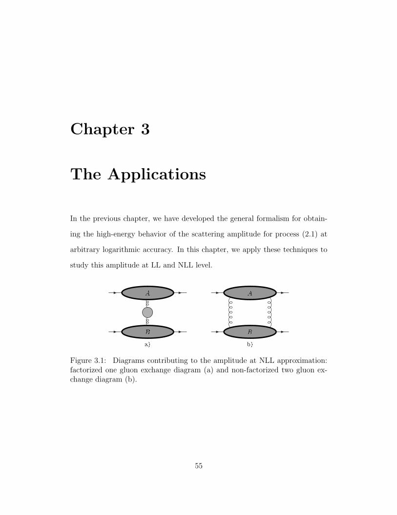
Chapter 3
The Applications
In the previous chapter, we have developed the general formalism for obtain-
ing the high-energy behavior of the scattering amplitude for process (2.1) at
arbitrary logarithmic accuracy. In this chapter, we apply these techniques to
study this amplitude at LL and NLL level.AB ABa) b)Figure 3.1: Diagrams contributing to the amplitude at NLL approximation:factorized one gluon exchange diagram (a) and non-factorized two gluon ex-change diagram (b).
55

3.1 Amplitude at LL
According to Eq. (2.58), the amplitude at LL comes solely from the factorized
diagram shown in Fig. 3.1a, but without any gluon self-energy corrections.
The jet A, containing lines moving in the plus direction, and jet B, consisting
of lines moving in the minus direction, interact via the exchange of a single soft
gluon. This gluon couples to jet A via the − component of its polarization and
to jet B via the + component of its polarization. Since vαA Nα β(q, η) vβ
B = 1,
we can write at LL
A8 b8 = −1
tJ
(1) aA (pA, q, η) J
(1)aB (pB, q, η), (3.1)
where b8 is the color basis vector corresponding to the octet exchange, defined
in Eq. (2.3). Using s = 2p+A p−B, the logarithmic derivative of the amplitude
can be expressed as
∂A8
∂ ln sb8 = −1
t
∂J(1) aA
∂ ln p+A
J(1) aB = −1
tJ
(1) aA
∂J(1) aB
∂ ln p−B. (3.2)
In Sec. 2.4.2, Eq. (2.33), we have derived an evolution equation resumming
ln(p+A) in J
(1)A . We note that J
(1)A = Γ
(1)A , and that (2.33) is a special case of the
evolution equation (2.51). The diagrammatic representation of the first term
on the far right hand side of Eq. (2.33), which follows from Fig. 2.4 in the
case when we have one external soft gluon attached to a jet function, is given
by the diagrams in Fig. 3.2. Diagram in Fig. 3.2a corresponds to Fig. 2.4b
and the diagrams in Figs. 3.2b and 3.2c correspond to Fig. 2.4a for n = 1.
The diagrams in Figs. 3.2b and 3.2c are in the factorized form, while the one
56

Ak + A + Aa) b) )
Figure 3.2: Diagrammatic representation of the evolution equation for jet J(1)A
at LL.
in Fig. 3.2a is not.
As discussed in Sec. 2.4.2, power counting shows that the loop momentum
k in Fig. 3.2a must be soft. This implies that we can make the following
approximations. First, since at LL all internal lines of the jet A are collinear
to the + direction, we can neglect the k+ dependence of J(2)A , i.e. we may
set k+ = 0 inside J(2)A . Also, we can pick the plus components of the vertices
where the soft gluons attach to the jet J(2)A . A short calculation, which uses
the Feynman rules for special lines and vertices listed in Appendix A.4, gives
the contribution to Fig. 3.2a in a form
Fig. 3.2a = −gs t facb
∫
dDk
(2π)D
1
k2(k − q)2 k · k vρANρµ(k)Sµ(k)
× vαBNαν(q − k)vν
A vβB vγ
B J(2) bc(A) β γ
(
pA, q, η; k+ = 0, k−, k⊥)
,
(3.3)
where we have defined gs ≡ gsµǫ. Using Eqs. (2.11) and (2.36) for the
components of the gluon propagator and the boxed vertex, respectively, it
is easy to see that in the Coulomb (Glauber) region, k− ≪ k+ ∼ k⊥, the
integrand in Eq. (3.3) becomes an antisymmetric function of k+ and that
57

vAa) b) )
Figure 3.3: Diagrams determining the contributions to the gluon trajectoryat the order αs.
therefore the integration over k+ vanishes in this region.
In the soft region, where all the components of soft momenta are of the
same size√−t, we can use the K-G decomposition for the soft gluon with
momentum k attached to J(2)A . At LL, however, there cannot be any soft
internal lines in J(2)A in Eq. (3.3), since, as discussed in Sec. 2.5.3, only
integrals over collinear momenta can produce powers of ln p+A. Therefore, at
LL, only the K gluon contributes, because the G gluon must be attached to
a soft line. The K gluon can be decoupled from the rest of the jet J(2)A using
the Ward identities, Eq. (2.30). Their application in Eq. (3.3) gives
Fig. 3.2a = −ig2sCAt
∫
dDk
(2π)D
1
k2(k − q)2 k · k vA · k vρANρµ(k)Sµ(k)
× vαBNαν(q − k)vν
A J(1) aA (pA, q, η). (3.4)
We have used the identity facb fdcb = Nc δad ≡ CA δad in Eq. (3.4). Eq. (3.4)
now gives a factorized form for Fig. 3.2a. Since the contributions in Figs. 3.2b
and 3.2c are already in the factorized form, we can immediately infer that the
gluon reggeizes at LL. Combining the terms from Fig. 3.2 in Eq. (2.33), we
58

obtain the evolution equation at leading logarithm
p+A
∂
∂p+A
J(1) aA (pA, q, η) = α(t) J
(1) aA (pA, q, η). (3.5)
Using the notation for evolution kernels introduced in Sec. 2.5.4, Eq. (3.5)
implies that
K(1,2;1) = 0. (3.6)
In Eq. (3.5)
α(t) ≡ 1 + α(1)a (t) + α
(1)b (t) + α(1)
c (t), (3.7)
is the gluon trajectory up to the order αs, and α(1)a (t), α
(1)b (t) and α
(1)c (t) are
its contributions given in Figs. 3.3a - 3.3c, respectively,
α(1)a (t) ≡ −ig2
sCAt
∫
dDk
(2π)D
1
k2(k − q)2 k · k vA · k vρANρµ(k)Sµ(k)
× vβBNβν(q − k)vν
A,
α(1)b (t) ≡ ig2
sCA
∫
dDk
(2π)D
1
k2(k − q)2 k · k Sα(k)Nα µ(k) vρAN ν
ρ (q − k)
× Vµβν(k,−q, q − k)vβB,
α(1)c (t) ≡ −ig2
sCA
∫
dDk
(2π)D
1
k2 k · k (q − k) · (q − k)vρ
ANρµ(k)Sµ(k) (vB · k) .
(3.8)
In Eq. (3.8), Vµβν(k,−q, q−k) stands for the momentum part of the three-
point gluon vertex. After contracting the tensor structures in Eq. (3.8), using
the explicit form for Vµβν , vA, vB, Sµ (Eq. (2.34)) and for the components of
59

the gluon propagator, Eq. (2.11), we obtain for α(1)a,b,c(t),
α(1)a (t) = −ig2
sCAt
2
∫
dDk
(2π)D
[k2⊥k0 + k2k3][(k − q)2 − (k − q)2
⊥]
(k0 + k3) k2 (k − q)2 (k · k)2 (k − q) · (k − q),
α(1)b (t) = ig2
sCA1
2
∫
dDk
(2π)D
1
k2 (k − q)2 (k · k)2 (k − q) · (k − q)
× [k2⊥ k2 (k − q)2 + 2k2 k2
3 (k − q)⊥ · q⊥ + 2k20 k2
3 k⊥ · (k − q)⊥ + 2k20 k2
⊥ (k − q)2⊥] ,
α(1)c (t) = ig2
sCA1
2
∫
dDk
(2π)D
k23
(k · k)2 (k − q) · (k − q). (3.9)
Next, we perform the k0 and k3 integrals in Eq. (3.9). For α(1)a (t), these
integrals are UV/IR finite. However in the case of α(1)b,c (t), the k0 integral is
linearly UV divergent. In order to regularize this energy integral, we invoke
split dimensional regularization introduced in Ref. [49]. The idea is to regu-
larize separately the energy and the spatial momentum integrals, i.e. to write
d4kE → dD1k4 dD2~k for Euclidean loop momenta kE. The dimensions D1 and
D2 are given by D1 = 1−2ε1 and D2 = 3−2ε2, with εj → 0+ for j = 1, 2. Since
the energy integral for α(1)c (t) is scaleless, it vanishes in this split dimensional
regularization. The energy integrals in α(1)a,b(t) are straightforward.
All the k3 integrals can be expressed as derivatives with respect to k2⊥
and/or (k − q)2⊥ of a single integral
I(a, b) ≡∫ ∞
0
dk3 1√
k23 + a2 (k2
3 + b2)=
1
b√
b2 − a2ln
(
b +√
b2 − a2
a
)
.
(3.10)
60

The result of these integrations over k3 is
α(1)a (t) = αsµ
2ǫ CA t
∫
dD−2k⊥(2π)D−2
×(
I(|k⊥|, |k⊥ − q⊥|)k2⊥
[(k − q)2⊥ − k2
⊥]2+
2(k − q)2⊥ − 3k2
⊥k2⊥ [(k − q)2
⊥ − k2⊥]2
)
,
α(1)b (t) = −αsµ
2ǫ CA t
∫
dD−2k⊥(2π)D−2
×(
I(|k⊥|, |k⊥ − q⊥|)k2⊥
[(k − q)2⊥ − k2
⊥]2− 1
[(k − q)2⊥ − k2
⊥]2
)
,
α(1)c (t) = 0. (3.11)
Combining the results of Eq. (3.11) and Eq. (3.7), we obtain the standard
expression for the gluon trajectory at LL
α(t) = 1 + CAαsµ2ǫ
∫
dD−2k⊥(2π)D−2
t
k2⊥ (k − q)2
⊥. (3.12)
We can now simply solve the evolution equation (3.2), to derive the factorized
(reggeized) form for the amplitude in the color octet
A8(s, t, αs) = sα(t) A8(t, αs). (3.13)
The amplitude factorizes into the universal factor sα(t), which is common for
all processes involving two partons in the initial and final state and dominated
by the gluon exchange, and the part A8, the so-called impact factor, which is
specific to the process under consideration.
61

3.2 Amplitude at NLL
At NLL level the contribution to the amplitude comes from both the one gluon
exchange diagram, Fig. 3.1a, and from the two gluon exchange diagram, Fig.
3.1b. At this level, both singlet and octet color exchange are possible in the
latter. Including the self-energy corrections to the propagator of the exchanged
gluon (taking into account the corresponding counter-terms), we can write the
contribution from the diagram in Fig. 3.1a as follows,
A(1) ≡ −1
tJ
(1) a(A) α (pA, q, η)
(
Nαβ(q, η) +1
tvα
B vµA Πµ ν(q, η) vν
B vβA
)
J(1) a(B) β (pB, q, η),
(3.14)
where Πµ ν(q, η) stands for the one loop gluon self-energy. We now put this
contribution into the first factorized form, Eq. (2.27), isolating the plus po-
larization for jet A, and the minus polarization for jet B. At NLL in the
amplitude, we need the soft function S(1,1), Eq. (2.27) with n = m = 1,
to accuracy O(αs). Using the tulip-garden formalism described in Appendix
A.3, the contribution to the first term on the right hand side of Eq. (3.14) is
given by the subtractions shown in Fig. 3.4. In accordance with the notation
adopted in Appendix A.3, the dashed lines indicate that we have made soft
approximations on gluons that are cut by them. A dashed line cutting a gluon
attached to jet A(B) means that the gluon is attached to the corresponding jet
through minus(plus) component of its polarization. Since q± = 0 in the Regge
limit, Eq. (2.2), we have Nµ±(q) = gµ±. This implies that the contributions
between the diagrams in Fig. 3.4c and in Fig. 3.4d as well as between the
diagrams in Fig. 3.4e and in Fig. 3.4f cancel each other. Therefore only the
62

AB NLL= AB + ABa) b) ) AB + AB ABd) e) f)Figure 3.4: Expansion of the one gluon exchange amplitude at NLL using thetulip garden formalism.
zeroth-order soft function diagram in Fig. 3.4b survives in the factorized form,
Eq. (2.27).
For the two gluon exchange, Fig. 3.1b, we only need the lowest order soft
function at NLL in the amplitude (and LL in singlet exchange). The expression
for the two gluon exchange diagram in Fig. 3.1b takes the form, Eq. (2.27),
A(2) =
∫
dDk
(2π)DJ
(2) a bA (k+ = 0, k−, k⊥) S(k+, k−, k⊥) J
(2) a bB (k− = 0, k+, k⊥),
(3.15)
where S(k) is given by
S(k) ≡ i
2!
N−+(k)
k2 + iǫ
N−+(q − k)
(q − k)2 + iǫ. (3.16)
We have suppressed the dependence of the functions appearing in Eq. (3.44)
on other arguments for brevity. At NLL accuracy we are entitled to pick the
plus Lorentz indices for jet function JA and the minus indices for jet function
63

JB only. We can also set k+ = 0 in JA and k− = 0 in JB since all the loop
momenta inside the jets are collinear. Eq. (3.44) represents the first factorized
form, Eq. (2.27), for the amplitude A(2).
Next, we follow the procedure described in Sec. 2.5.1 to bring the amplitude
into the second factorized form, Eq. (2.40). We employ an identity based on
Eq. (2.44), for the function S(k) defined in Eq. (3.16)
S(k+, k−) = S(k+ = 0, k− = 0) θ(M − |k+|) θ(M − |k−|)
+ [S(k+, k− = 0) − S(k+ = 0, k− = 0) θ(M − |k+|)] θ(M − |k−|)
+ [S(k+ = 0, k−) − S(k+ = 0, k− = 0) θ(M − |k−|)] θ(M − |k+|)
+ [S(k+, k−) − S(k+, k− = 0) θ(M − |k−|) −
S(k+ = 0, k−) − S(k+ = 0, k− = 0) θ(M − |k−|) θ(M − |k+|)].
(3.17)
The contribution from the first term in Eq. (3.17) gives immediately the
second factorized form with Γ(2)A and Γ
(2)B defined in Eq. (2.41) for n = m = 2.
We now discuss the rest of the terms in Eq. (3.17), which can be analyzed
using the K-G decomposition, since, by construction, there is no contribution
from the Glauber region. At the current accuracy only the K-gluon con-
tributes. After substituting the second term of Eq. (3.17) into Eq. (3.44),
we can factor the gluon with momentum k from jet J(2)B . However, it is easy
to verify, using the definitions for K and G gluons, Eq. (2.29), the Ward
identities, Eq. (2.30), and the explicit components of the gluon propagator,
Eq. (2.11), that the k+ integral is over an antisymmetric function. As a re-
64

sult, this contribution vanishes. In a similar fashion, the contribution from
the third term in Eq. (3.17), after used in Eq. (3.44), vanishes, since now we
can factor the soft gluon with momentum k from jet J(2)A and the k− integral
is over an antisymmetric function.
In the case of the last term in Eq. (3.17), after used in Eq. (3.44), we
can factor the soft gluon with momentum k from both jets J(2)A and J
(2)B . The
integrals of the soft function S(k) over k+ and k− are then
S(k⊥, q; M) ≡ CAg2
s
(2π)2
∫ M
−M
dk+
k+
dk−
k− S(k+, k−, k⊥, q). (3.18)
As usually, we leave the transverse momentum integral undone. The 1/k+
and 1/k− in the integral above are given by the Principal Value prescription
because there is no contribution from the Glauber region. Since the amplitude
is independent on the choice of scale M , we can evaluate it at arbitrary scale.
We choose to work in the limit M → 0. In this limit the contribution to
the integral comes from the imaginary parts of the gluon propagators in Eq.
(3.16), −iπδ(k2) and −iπδ((k − q)2). The integration is then trivial and Eq.
(3.18) becomes
S(k⊥, q) ≡ limM→0
S(k⊥, q; M) ≡ −CAig2
s
8
1
k2⊥ (k − q)2
⊥. (3.19)
Combining the partial results of the analysis described above in Eq. (3.44), we
arrive at the second factorized form for the double gluon exchange amplitude,
65
Fig. 3.1b,
A(2) =
∫
dD−2k⊥(2π)D−2
Γ(2) a bA (k⊥)
1
(2π)2S(k+ = 0, k− = 0, k⊥) Γ
(2) a bB (k⊥)
+
∫
dD−2k⊥(2π)D−2
Γ(1) aA (pA, q) S(k⊥, q) Γ
(1) aB (pA, q). (3.20)
Using Eq. (3.14) for A(1) and Eq. (3.20) for A(2), we obtain the amplitude for
the process (2.1) at NLL accuracy
A(NLL) = −1
tΓ
(1) aA (pA, q, η)
(
1 +1
tΠ+−(q, η) +
iπ
2α(1)(t)
)
Γ(1) aB (pB, q, η)
+
∫
dD−2k⊥(2π)D−2
Γ(2) a bA (k⊥)
i
8π2
1
k2⊥ (k − q)2
⊥Γ
(2) a bB (k⊥). (3.21)
In Eq. (3.21), we have used the explicit form for S(k+ = 0, k− = 0, k⊥),
which can be easily identified from Eq. (3.16). We have also used the integral
representation of the gluon trajectory given in Eq. (3.12).
In order to determine the high energy behavior of the amplitude in Eq.
(3.21), we need to examine the high energy behavior of Γ(1)A or Γ
(1)B at NLL
and the evolution of Γ(2)A or Γ
(2)B at LL. In this section, we restrict the discussion
of evolution equations to LL level, and hence we analyze the behavior of Γ(2)A
only. We will address the study of NLL jet evolution, and gluon reggeization
at this level in the next section.
We use the evolution equation given by Eq. (2.51) in order to determine
the LL dependence of Γ(2)A on ln(p+
A). In our special case of the two gluon
66

+ Ak q kl G + Ak q kl G + Ak q kq la) b) )+ Ak q kl + A
k q kl Alk q kd) e) f)Figure 3.5: Diagrams determining the evolution of Γ
(2)A .
exchange amplitude, it reads
(
p+A
∂
∂ p+A
− 1
)
Γ(2) a bA = M
[
J(2) a bA (k− = +M, k+ = 0, k⊥)
+ J(2) a bA (k− = −M, k+ = 0, k⊥)
]
− ηα ∂
∂ ηαΓ
(2) a bA .
(3.22)
The first term in Eq. (3.22) can be analyzed using the K-G decomposition.
The contributions from the K-gluon cancel between the J(2)A (k− = +M) and
J(2)A (k− = −M). The contributions from the G gluon, which we now discuss,
are shown in Figs. 3.5a and 3.5b.
Since the gluon with momentum q−k in Fig. 3.5a cannot be in the Glauber
region, we can use K-G decomposition on it. The K part factors from J(3)A ,
while the G part does not contribute at LL. After factoring out the gluon with
momentum q − k and performing the approximations on the jet function J(2)A ,
67

the contribution to Fig. 3.5a for k− = +M is
Fig. 3.5a = −ig2sfaecfdeb
1
M
∫
dDl
(2π)DS1(k
+ = 0, k− = +M, k⊥, l)
× J(2) c dA (l+ = 0, l−, l⊥), (3.23)
where we have defined
S1(k, l) ≡ N−µ(l)
l2N− ν(k − l)
(k − l)2Vµ ρ ν(l,−k, k − l)
(
gρ+ − kρ
M
)
. (3.24)
Next we follow the established procedure. First, we write
S1(k, l) = S1(k, l− = 0) θ(M − |l−|) +[
S1(k, l) − S1(k, l− = 0) θ(M − |l−|)]
.
(3.25)
When we use the second term of Eq. (3.25) in Eq. (3.23), we can factor
the gluon with momentum l from J(2)A . Since the resulting integrand is an
antisymmetric function under the simultaneous transformation M → −M ,
l± → −l±, the contributions on the right hand side of Eq. (3.22) evaluated
for k− = +M and k− = −M cancel each other. Therefore we can write, using
Eq. (3.25) in Eq. (3.23),
Fig. 3.5a = −ig2s faecfdeb
1
M
∫
dD−2l⊥(2π)D
∫
dl+
× S1(k+ = 0, k− = +M, k⊥, l− = 0, l+, l⊥) Γ
(2) c dA (l⊥) + . . . ,
(3.26)
where by dots we mean the term which is canceled after we take into account
68

the contributions to both J(2)A (k− = +M) and J
(2)A (k− = −M) on the right
hand side of Eq. (3.22).
Next, we perform the l+ integral in Eq. (3.26). As we have already men-
tioned above, since the final result does not depend on the scale M , we can
choose arbitrary value of M . We have chosen to perform the calculation in
the limit M → 0. Then the only non-vanishing contribution comes from the
imaginary part of the propagator 1/[(l−k)2 + iǫ], −iπ δ(2Ml+ +(l−k)2⊥). For
this term the l+ integration is trivial and we obtain
M (Fig. 3.5a) = −αs faecfdeb
∫
dD−2l⊥(2π)D−2
2k⊥ · l⊥l2⊥ (k − l)2
⊥Γ
(2) c dA (l⊥) + . . . , (3.27)
which gives an M-independent contribution to the right hand side of Eq.
(3.23).
We follow the same steps when dealing with the diagram in Fig. 3.5b,
whose soft sub-diagram is given by
S2(k, l) ≡ N−µ(l)
l2N− ν(q − l)
(q − l)2Vµ ρ γ(l,−k, k − l)
(
gρ+ − kρ
M
)
Nγδ(l − k)
(l − k)2
× Vν δ −(q − l, l − k, k − q). (3.28)
First we use the identity (3.25) for S2. The contribution due to the second term
in Eq. (3.25) vanishes, after the gluon with momentum l has been factored
from J(2)A , due to the antisymmetry of the integrand. Hence again, as in the
case discussed above, only the term given by S2(l− = 0, l+, l⊥, k) contributes.
In the limit M → 0, the contribution comes from the imaginary part of the
69

same denominator as in the case of Fig. 3.5a. The result is
M (Fig. 3.5b) = − αs faecfdeb
∫
dD−2l⊥(2π)D−2
2
l2⊥ (l − q)2⊥ (k − l)2
⊥
×(
k2⊥l2⊥ − k⊥ · l⊥l2⊥ − k⊥ · q⊥l2⊥ − k2
⊥l⊥ · q⊥ + 2k⊥ · l⊥l⊥ · q⊥)
× Γ(2) c dA (l⊥) + . . . . (3.29)
Combining the results of Eqs. (3.27) and (3.29), we obtain the expression for
the surface term in Eq. (3.22)
M [ J(2) a bA (k− = +M, k+ = 0, k⊥) + J
(2) a bA (k− = −M, k+ = 0, k⊥) ]
= 2αs faecfbed
∫
dD−2l⊥(2π)D−2
(
k2⊥
l2⊥ (k − l)2⊥
+(k − q)2
⊥(l − q)2
⊥ (k − l)2⊥− q2
⊥l2⊥ (q − l)2
⊥
)
×Γ(2) c dA (l⊥). (3.30)
Next, we analyze the contributions to the term ηα∂/∂ ηα Γ(2)A in the evo-
lution equation (3.22). The contributing diagrams are shown in Figs. 3.5c -
3.5f. Note that for every diagram in Figs. 3.5c - 3.5f, we have also diagrams
when a loop containing the boxed vertex is attached to the external gluon with
momentum k, instead of to the external gluon with momentum q − k.
In Fig. 3.5c, we have to consider all the possible insertions of external
gluons with momenta k and q−k. We have six possibilities. The contribution
shown in Fig. 3.5c is proportional to (omitting the color factor)
∫ M
−M
dk− (Fig. 3.5c) ∝∫ M
−M
dk−∫
dDl
(2π)D
N−µ(l)
l2Sµ(l)
l · l(l − k)+
(l − k)2
(q − l)+
(q − l)2(k+ = 0).
(3.31)
Since the integrand is an antisymmetric function under k− → −k− and l± →
70

+ Alk q k A lk q k Al kk q ka) b) ) Al kk q k A l kq k + A lk q kd) e) f)Figure 3.6: Contributions to the diagram in Fig. 3.5f when the gluon comingout of the boxed vertex is attached to the soft line (a) and when either or bothgluons with momenta k and l are K gluons and they are factored from the jet(b - f).
−l±, the integral in Eq. (3.31) vanishes. The same antisymmetry property
holds for the remaining five diagrams and therefore, there is no contribution
from them.
Let us next focus on the diagram in Fig. 3.5f. When the gluon with
momentum l attaches to a soft line inside of the jet J(3)A , the contribution
takes the form shown in Fig. 3.6a. If it attaches to a jet line, its contribution
can be written as
Fig. 3.5f = −gsfbcd
∫
dDl
(2π)DS3(k
+ = 0, k−, k⊥, l)
× J(3) a c dA (k+ = 0, k−, k⊥, l+ = 0, l−, l⊥), (3.32)
71
with the soft function
S3(k, l) ≡ (q − k)2 N−µ(l)
l2Sµ(l)
l · lN−+(q − k − l)
(q − k − l)2. (3.33)
We use the identity for this soft function S3, obtained from Eq. (3.17) by the
replacement k+ → l−,
S3(l−, k−) = S3(l
− = 0, k− = 0) θ(M − |l−|) θ(M − |k−|)
+ [S3(l−, k− = 0) − S3(l
− = 0, k− = 0) θ(M − |l−|)] θ(M − |k−|)
+ [S3(l− = 0, k−) − S3(l
− = 0, k− = 0) θ(M − |k−|)] θ(M − |l−|)
+ [S3(l−, k−) − S3(l
−, k− = 0) θ(M − |k−|)
− S3(l− = 0, k−) − S3(l
− = 0, k− = 0) θ(M − |k−|) θ(M − |l−|)],
(3.34)
to treat the soft gluons with momenta k and l attached to jet J(3)A . The con-
tribution from the first term in Eq. (3.34), when used in Eq. (3.32), vanishes
since the integrand S3(k+ = k− = 0, k⊥, l− = 0, l+, l⊥) is an antisymmetric
function of l+, as can be easily checked using Eqs. (2.11), (2.36) and (B.35).
We can apply the K-G decomposition on the gluon with momentum l when
treating the second term in Eq. (3.34) used in Eq. (3.32). At LL only the
K gluon contributes. It can be factored from the jet function J(3)A with the
result shown in Figs. 3.6b and 3.6c. In a similar way we can treat the gluon
with momentum k in the third term of Eq. (3.34). After we factor this gluon
from the jet J(3)A , we obtain the contributions shown in Figs. 3.6d and 3.6e.
In the case of the last term in Eq. (3.34), we can factor out both soft gluons
72

with momenta k and l from jet J(3)A . The result of this factorization is shown
in Fig. 3.6f.
Next, we note that the combination of the diagrams in Figs. 3.5d, 3.5e and
3.6b is the same as the result encountered in the analysis of the LL amplitude,
Fig. 3.3. We write
∫ M
−M
dk− (Fig. 3.5d + Fig. 3.5e + Fig. 3.6b) = α(1)(q⊥ − k⊥) Γ(2) a bA (pA, q, k⊥).
(3.35)
where α(1)(q − k) in Eq. (3.35) is given by the diagrams in Fig. 3.3 with an
external momentum q − k = (0+, 0−, q⊥ − k⊥). In the case when the gluon
coming out of the boxed vertex attaches to an external gluon with momentum
k, we evaluate the one loop trajectory α(1)(k⊥) in Eq. (3.35).
To complete the analysis, we have to discuss the diagrams in Figs. 3.6a
and 3.6c - 3.6f. In the region l± ∼ l⊥, we can factor the gluon with momentum
l from the jet function J(2)A (l+ = 0, l−, l⊥) in the case of the diagram in Fig.
3.6a. The resulting k− and l± integral is over an antisymmetric function of
k− and l±, and therefore it vanishes. So the only contribution comes from the
Glauber region, where we can set l− = 0 outside J(2)A (l+ = 0, l−, l⊥). As above,
we perform the l+ and k− integrals in the limit M → 0. The integrand does
not develop a singularity in k− and/or l+ strong enough to compensate for the
shrinkage of the integration region∫M
−Mdk− when M → 0. Hence the diagram
in Fig. 3.6a does not contribute in the limit M → 0. In a similar way as for
the diagram in Fig. 3.6a, none of the diagrams in Figs. 3.6c - 3.6f contribute.
The diagrams in Figs. 3.6c - 3.6e vanish in the M → 0 limit, while in the case
of the diagram in Fig. 3.6f the k− and l± integral is over an antisymmetric
73
function of k− and l±.
At this point we have discussed all the contributions appearing on the right
hand side of the evolution equation (3.22). Combining the partial results given
by Eqs. (3.35) and (3.30) in Eq. (3.22), we arrive at the evolution equation
governing the high energy behavior of Γ(2)A
(
p+A
∂
∂ p+A
− 1
)
Γ(2) a bA (p+
A, q, k⊥) = 2αs faecfbed
∫
dD−2l⊥(2π)D−2
Γ(2) c dA (p+
A, q, l⊥)
×(
k2⊥
l2⊥ (k − l)2⊥
+(k − q)2
⊥(l − q)2
⊥ (k − l)2⊥− q2
⊥l2⊥ (q − l)2
⊥
)
+(
α(1)(k⊥) + α(1)(q⊥ − k⊥))
× Γ(2) a bA (p+
A, q, k⊥).
(3.36)
Projecting out onto the color singlet in Eq. (3.36), we immediately recover
the celebrated BFKL equation [21].
3.2.1 Evolution of Γ(n) at LL
We can now generalize Eq. (3.36) to the case of Γ(n)A . The evolution kernel in
this case contains, besides a piece diagonal in the number of external gluons,
also contributions which relate jet functions with different number of external
74

gluons
(
p+A
∂
∂ p+A
− 1
)
Γ(n) a1... an
A (p+A, q, k1⊥, . . . , kn⊥) =
2αs
n∑
i<j
fai e bifaj e bj
∫
dD−2li⊥(2π)D−2
dD−2lj ⊥(2π)D−2
δ(2)(li⊥ + lj ⊥ − ki⊥ − kj ⊥)
×(
k2i⊥
l2i⊥ (ki − li)2⊥
+k2
j ⊥l2j ⊥ (kj − lj)
2⊥− (ki + kj)
2⊥
l2i⊥ l2j ⊥
)
× Γ(n) a1... bi... bj ... an
A (p+A, q, k1⊥, . . . , li⊥, . . . , lj ⊥, . . . , kn⊥)
+
n∑
i=1
(
α(1)(ki⊥))
× Γ(n) a1... an
A (p+A, q, k1⊥, . . . , kn⊥)
+
n−1∑
n′=1
K(n,n′)a1... an; b1... bn′
⊗⊥ Γ(n′) b1... bn′
A , (3.37)
where ⊗⊥ denotes a convolution in transverse momentum space. The last term
in Eq. (3.37) corresponds to the configurations when one or more external
gluons attach to a gluon or a ghost lines forming the one loop kernel derived
for Γ(2)A . Using the notation of Sec. 2.5.4, we can write Eq. (3.37) at r-loop
order in a form
(
p+A
∂
∂p+A
− 1
)
Γ(n,r)A =
n∑
n′=1
K(n,n′;1) ⊗ Γ(n′,r−1)A . (3.38)
It corresponds to Eq. (2.64) of Sec. 2.5.4 when written in terms of the coef-
ficients c(n,r)r introduced in Eq. (2.60). From Eq. (3.38) we immediately see
that the following property of the one loop kernel
K(n,n′;1) = θ(n − n′) K(n,n′;1), (3.39)
75

is satisfied. We recall that this step was essential in demonstrating that the
set of evolution equations, Eq. (2.51), forms a consistent system, refer to the
paragraph above Eq. (2.64).
The term diagonal in the number of external gluons in Eq. (3.37) coin-
cides with the evolution equation derived in Ref. [17]. Our formalism, besides
enabling us to go systematically beyond LL accuracy, indicates that even at
LL, in addition to the kernels found in Ref. [17], the kernel has contributions
which relate jet functions with different number of external gluons.
3.3 Gluon reggeization at NLL
In this section, we study the NLL evolution equation and the gluon reggeiza-
tion. In Sec. 3.3.1, we identify the contributions to the amplitude at NLL
and negative signature channel. Sec. 3.3.2 gives a detailed derivation of the
relevant evolution equation.
3.3.1 Color octet and negative signature amplitude
The statement of gluon reggeization means that the scattering amplitude in the
Regge limit, dominated by the gluon exchange (color octet) in the t-channel,
and antisymmetric under s ↔ u (negative signature), takes the form
A(−)8
(s, t) rArB ,r1r2 = F aA(t) r1rA
[
(
s
−t
)α(t)
−(−s
−t
)α(t)]
F aB(t) r2rB
, (3.40)
where F aA(t) and F a
B(t) are the impact factors, which depend on the properties
of the scattered particles. The Regge trajectory α(t) determines the depen-
76

PAPBP1P2AB A0B0 PAPB
P1P2A0B AB0Figure 3.7: Projection of the amplitude onto the negative signature channel.
dence on the energy√
s. It is a universal function of t meaning that it does
not depend on the particles involved in the scattering. In order to project onto
the negative signature channel, besides the amplitude for qq′ → qq′ scattering,
Eq. (2.1), we consider the amplitude for the process
q(pA, r1, λA) + q′(pB, rB, λB) → q(pA − q, rA, λ1) + q′(pB + q, r2, λ2). (3.41)
The amplitude for scattering (3.41), A(s, t), can be obtained from the ampli-
tude for the process (2.1), A(s, t), by the crossing symmetry s ↔ u. This
means that A(s, t) = A(u, t) ≃ A(−s, t). Hence, if we define
A(−)(s, t) ≡ 1
2
(
A(s, t) − A(s, t))
, (3.42)
as indicated in Fig. 3.7, the amplitude A(−) will have a negative signature by
construction. Since s ∼ −u in the Regge limit, the logarithmic derivative of
this amplitude is:
∂A(−)
∂ ln s(s, t) =
1
2
(
s∂A
∂s(s, t) − u
∂A
∂u(s, t)
)
, (3.43)
We now isolate the negative signature contribution to the amplitude for
77

process (2.1) at NLL. The projection of the set of two gluon exchange diagrams,
Fig. 3.1b, onto the negative signature takes the form:
A(−)2 =
∫
dDk
(2π)D
[
J(2) a bA (k+ = 0, k−, k⊥) − J
(2) a bA (k+ = 0, k−, k⊥)
]
× S(k+, k−, k⊥) × J(2) a bB (k− = 0, k+, k⊥), (3.44)
where S(k) has been defined in Eq. (3.16) and J(2)A is the jet function corre-
sponding to the anti-quark in the process (3.41) moving in the plus direction.
In Appendix B.1 we show that the jet functions J(n)A and J
(n)A are related by
the symmetry:
J(n)A (k+
i → −k+i , k−
i → −k−i , ki⊥ → ki⊥) = (−1)n−1 (−1)λA+λ1 J
(n)A (k+
i , k−i , ki⊥),
(3.45)
in the Regge limit. Applying this identity to the jet function with two external
gluons (n = 2), the helicity conserving part of the jet function (λA + λ1 =
2λA = ±1) obeys:
J(2)A (k+ = 0,−k−, k⊥) = J
(2)A (k+ = 0, k−, k⊥). (3.46)
We apply this result to analyze Eq. (3.44). Using Eqs. (3.16) and (3.46),
we easily see that in the Glauber region k− ≪ k+ ∼ k⊥ the integrand in Eq.
(3.44) is over an antisymmetric function of k− and therefore the k− integral
vanishes. This indicates that there is no contribution from the Glauber region
when analyzing a soft gluon with momentum k in Fig. 3.2b and therefore this
gluon can be factored from the jet functions J(2)A and J
(2)B . As a consequence,
78

the high-energy behavior of the amplitude for the process (2.1), projected
onto the negative signature channel, is determined by the jet functions with
one external gluon only, J(1)A and J
(1)B . It also means that A
(−)2 is automatically
in the color octet channel.
Combining the contributions from the one and the two gluon exchange
diagrams shown in Fig. 3.1, the negative signature amplitude A(−)8
takes the
form:
A(−)8
= −1
t
(
J(1) aA (pA, q, η) − J
(1) aA (pA, q, η)
)
(
1 +1
tΠ+−(q, η) +
iπ
2α(1)(t)
)
× J(1) aB (pA, q, η), (3.47)
where Π+−(q, η) is the one-loop gluon self-energy and α(1)(t) is the one-loop
contribution to the gluon trajectory given in Eq. (3.12). Eq. (3.47) indicates
that in order to determine the high energy behavior of the scattering ampli-
tude, we need to determine the high-energy behavior of J(1)A and J
(1)A . If we
show that J(1)A and J
(1)A satisfy:
p+A
∂J(1)A
∂p+A
= α(t) J(1)A ,
p+A
∂J(1)A
∂p+A
= α(t) J(1)A , (3.48)
at NLL, then the solution to the evolution equation (3.48) used in Eqs. (3.43)
and (3.47) implies the Regge ansatz, Eq. (3.40). This would provide a proof
of gluon reggeization at NLL to all orders in perturbation theory in QCD,
Ref. [28]. We study the evolution equation (3.48) in the next section.
79

Ak Ak Ak l + Aa) b) ) d)
Figure 3.8: Diagrammatic representation of the evolution equation for jet J(1)A
at NLL.
3.3.2 NLL evolution equation for J(1)A
We now derive the evolution equation for jet function J(1) aA at NLL. We restrict
ourselves to J(1)A since J
(1)A can be analyzed in the same way. Applying the
general evolution equation, Eq. (2.51), for n = 1 and using the results in Fig.
2.4, we arrive at the contributions to (∂/∂ ln p+A − 1)J
(1) aA shown in Fig. 3.8.
The diagram in Fig. 3.8d, is already in a factorized form so it does not need to
be analyzed further. The blob in the bottom part of this diagram represents
all possible two loop corrections.
In Fig. 3.8b, the bottom dark blob denotes the one loop gluon-self energy.
The gluon with momentum k can be analyzed the same way as in the case of
LL, Sec. 3.1, with a result in a factorized form.
In order to prove reggeization of a gluon at NLL, we need to show that the
soft gluon with momentum k in Fig. 3.8a and the soft gluons with momenta
k and l in Fig. 3.8c can be factored from the jet functions J(2)A and J
(3)A ,
respectively. Let us now analyze these particular diagrams. The contribution
to Fig. 3.8a can be written
Fig. 3.8a = −igsfabc
∫
dDk
(2π)DSµ ν(k, q) J
(2) µ ν(A) b c (pA, q; k). (3.49)
80

Ak q AvAlk q
AvAlk qa) b) )Figure 3.9: Contributions to Fig. 3.8a from the K gluon at NLL.
Next, we use the following identity for the integrand in Eq. (3.49)
Sµ ν(k) J(2) µ ν(A) b c (k) = S++(k) J
(2) + +(A) b c (k+ = 0, k−, k⊥)
+[
S++(k) J(2) + +(A) b c (k) − S++(k) J
(2) ++(A) b c (k+ = 0, k−, k⊥)
]
+[
Sµ ν(k) J(2) µ ν(A) b c (k) − S+ +(k) J
(2) + +(A) b c (k)
]
. (3.50)
The first term in Eq. (3.50), after being inserted into Eq. (3.49), can be
analyzed using the K-G decomposition, since there is no contribution from
the Glauber region due to the antisymmetry of S+ +(k+, k− = 0, k⊥) under
the transformation k+ → −k+. The contributions from the K gluon, after
applying the Ward identities, can be expressed in a form shown in Fig. 3.9.
The diagram in Fig. 3.9a is the same as in the case of LL. At NLL, we also have
to insert the gluon and ghost self-energies where appropriate. This diagram
is in a factorized form and therefore consistent with a gluon reggeization at
NLL.
As for diagrams in Figs. 3.9b and 3.9c, the gluon with momentum l can
be factored from the jet function J(2)A as shown in Appendix B.2. Thus the
contributions from the K gluon in Figs. 3.9a - 3.9c can be written in a factor-
ized form and they are in an agreement with the gluon reggeization at NLL.
81

Akl Al q k Akla) b) )Ak l Ak l Ak ld) e) f)Figure 3.10: Soft contributions to Figs. 3.8a and 3.8c.
Next, we analyze the contributions from the G gluon with momentum k cor-
responding to the first term in Eq. (3.50) and to Fig. 3.8a. They come from
the diagrams shown in Figs. 3.10a, 3.10c and 3.10d since the G gluon must
be attached to a soft line. In Appendix B.2, we show that the soft gluons
with momenta l and k − l can be factored from the jet function J(3)A in Fig.
3.10a, the soft gluons with momenta l can be factored from the jet functions
J(2)A in Figs. 3.10c and 3.10d and therefore the contribution from the G gluon
corresponding to Fig. 3.8a is in a factorized form.
Now, we examine the gluons with momenta k and/or q − k in the second
and the third terms of Eq. (3.50), after used in Eq. (3.49). They must attach
to soft lines and therefore the typical contributions to these terms come from
diagrams shown in Figs. 3.10a - 3.10d. First we analyze the contributions to
the second term in Eq. (3.50). As shown in Appendix B.2, the contribution
to the diagram in Fig. 3.10c is in a factorized form. However, there are
82
contributions to the diagrams in Fig. 3.10a and Fig. 3.10b, coming from
the region when all soft gluons external to J(3)A are Glauber, which cannot be
written in a simple factorized form. These contributions, Eq. (B.20) and Eq.
(B.24), are rather in a form of a convolution in transverse momentum space.
As far as the last term in Eq. (3.50) is concerned, its contributions come
from the diagrams in Figs. 3.10a - 3.10d. As we demonstrate in Appendix
B.2, the soft gluons external to J(3)A in Figs. 3.10a and 3.10b, as well as the
soft gluons external to J(2)A in Figs. 3.10c and 3.10d can be factored from the
the jet functions.
Finally, we need to examine the diagram in Fig. 3.8c which can be written
as
Fig. 3.8c ≡∫
dDk
(2π)D
dDl
(2π)DSb c d(k, l, q)
× J(3) b c dA (pA, q; k+ = 0, k−, k⊥, l+ = 0, l−, l⊥)
+
∫
dDl
(2π)DSb c(l, q) J
(2) b cA (pA, q; l+ = 0, l−, l⊥)
+
∫
dDk
(2π)DSb c(k, q) J
(2) b cA (pA, q; k+ = 0, k−, k⊥). (3.51)
The contribution to the first term in Eq. (3.51) comes from a diagram shown
in Fig. 3.8c where the soft gluons with momenta k, l and q−k− l attach to jet
lines inside the jet function J(3)A . At NLL we can set k+ = l+ = 0 inside J
(3)A
and also the soft gluons attach to the plus components of the jet’s vertices. As
shown in Appendix B.2, in the region when both gluons with momenta k and
l are Glauber, we cannot factor out these gluons and the contribution from
this double Glauber region is not in a factorized form.
83

The contribution to the last two terms in Eq. (3.51) comes from the graphs
shown in Figs. 3.10e and 3.10f, respectively. The gluon with momentum
q−k− l attaches to soft gluons with momenta k, Fig. 3.10e, and l, Fig. 3.10f,
respectively. In Appendix B.2 we demonstrate that the gluons external to J(2)A ,
can be factored from the jet functions J(2)A .
As a result of the previous reasoning, we arrive at a conclusion that the
evolution equation for the jet function J(1)A at NLL takes the form:
p+A
∂J(1) aA
∂p+A
(pA, q) = K(1,1)(t) J(1) aA (pA, q) +
∫
dD−2k⊥(2π)D−2
dD−2l⊥(2π)D−2
K(1,3)abcd (q, k⊥, l⊥)
× Γ(3) b c dA (pA, q; k⊥, l⊥). (3.52)
The kernel K(1,1) is given by all the diagrams where it was possible to factor
the soft gluons from the jet functions. This piece is in an agreement with
gluon reggeization at NLL according to Eq. (3.48). Besides this term, there
is a contribution in Eq. (3.52) corresponding to the configurations when all
soft gluons external to the jet function J(3)A are Glauber. Combining the re-
sults of Eqs. (B.20), (B.24) and (B.39) in Appendix B.2, we can find out the
explicit form of the kernel K(1,3). The presence of this term in Eq. (3.52)
suggests the breakdown of gluon reggeization at NLL level. We have to note
the following, however. At two loop level, these non-factorizing terms vanish.
The non-factorizing piece in every diagram comes from the double pinched
region, corresponding to the two delta function terms originating from the
two denominators on the fermion line present in the tree-level jet function.
They, however, do not produce any dependence on transverse momenta and
therefore this term is symmetric in external momenta. Hence if we inter-
84

change the two external momenta flowing out of J(3)A and into the three point
gluon-gluon-gluon or ghost-gluon-ghost vertex, Figs. 3.10a, 3.10b and 3.8c, the
integrand becomes an antisymmetric function under this exchange and the in-
tegral vanishes. However, when the jet function contains loop corrections, it
will, in general, not be symmetric under the interchange of external momenta
only. In order to get the symmetry, we need to interchange the colors as well.
Nevertheless, the above argument shows that the standard analysis and the
calculations which have been performed at the two loop level, Refs. [26] - [33],
are not in a contradiction with our results.
3.4 Conclusions
As an illustration of the general algorithm we have demonstrated it in an
action at NLL in both the amplitude and the evolution equations. First, in
Sec. 3.1, we have performed the resummation of the amplitude at LL. We
have found the standard expression for the gluon Regge trajectory, Eq. (3.12).
Then, in Sec. 3.2, we have identified the class of diagrams contributing to the
amplitude at NLL level. They involved one and two gluon exchange diagrams,
Fig. 3.1. The resummation of the two gluon exchange diagram in Sec. 3.2,
needed to be performed at LL. It has lead to the celebrated BFKL equation,
Eq. (3.36). The one gluon exchange contribution had to be resummed at
NLL. Together with this resummation, we have addressed the question of
gluon reggeizaiton at NLL in Sec. 3.3. We have found that the majority of the
terms in the evolution kernel are in an agreement with this conjecture to all
orders in perturbation theory. However, we have also identified contributions
85
violating the Regge ansatz starting at the three loop level and calculated the
corresponding evolution kernels, Eqs. (B.20), (B.24), (B.39). We have not
been able to prove that these contributions decouple from the jets. A further
study of symmetries involving jets with three external gluons should shed more
light on the presence or absence of the non-factorized terms, Ref. [11].
86

Part II
Resummation in Dijet Events
87

Chapter 4
Event Shape / Energy Flow
Correlations
4.1 Introduction
The agreement of theoretical predictions with experiment for jet cross sections
is often impressive. This is especially so for inclusive jet cross sections at high
pT , using fixed-order factorized perturbation theory and parton distribution
functions [52]. A good deal is also known about the substructure of jets,
through the theoretical and experimental study of multiplicity distributions
and fragmentation functions [53], and of event shapes [54–56]. Event shape
distributions [57–59] in particular offer a bridge between the perturbative,
short-distance and the nonperturbative, long-distance dynamics of QCD [60].
Energy flow [61] into angular regions between energetic jets gives informa-
tion that is in some ways complementary to what we learn from event shapes.
In perturbation theory, the distribution of particles in the final state reflects
88
interference between radiation from different jets [53], and there is ample evi-
dence for perturbative antenna patterns in interjet radiation at both e+e− [62]
and hadron colliders [63, 64]. Energy flow between jets must also encode the
mechanisms that neutralize color in the hadronization process, and the tran-
sition of QCD from weak to strong coupling. Knowledge of the interplay
between energy and color flows [65,66] may help identify the underlying event
in hadron collisions [67], to distinguish QCD bremsstrahlung from signals of
new physics. Nevertheless, the systematic computation of energy flow into
interjet regions has turned out to be subtle [68] for reasons that we will review
below, and requires a careful construction of the class of jet events. It is the
purpose of this work to provide such a construction, using event shapes as a
tool.
In this paper, we introduce correlations between event shapes and energy
flow, “shape/flow correlations”, that are sensitive primarily to radiation from
the highest-energy jets. So long as the observed energy is not too small, in
a manner to be quantified below, we may control logarithms of the ratio of
energy flow to jet energy [66, 69].
The energy flow observables that we discuss below are distributions asso-
ciated with radiation into a chosen interjet angular region, Ω. Within Ω we
identify a kinematic quantity QΩ ≡ εQ, at c.m. energy Q, with ε ≪ 1. QΩ
may be the sum of energies, transverse energies or related observables for the
particles emitted into Ω. Let us denote by Ω the complement of Ω. We are
interested in the distribution of QΩ for events with a fixed number of jets in
89
Ω. This set of events may be represented schematically as
A + B → Jets + XΩ + RΩ(QΩ) . (4.1)
Here XΩ stands for radiation into the regions between Ω and the jet axes, and
RΩ for radiation into Ω.
The subtlety associated with the computation of energy flow concerns the
origin of logarithms, and is illustrated by Fig. 4.1. Gluon 1 in Fig. 4.1 is an
example of a primary gluon, emitted directly from the hard partons near a jet
axes. Phase space integrals for primary emissions contribute single logarithms
per loop: (1/QΩ)αns lnn−1(Q/QΩ) = (1/εQ)αn
s lnn−1(1/ε), n ≥ 1, and these
logarithms exponentiate in a straightforward fashion [66]. At fixed QΩ for
Eq. (4.1), however, there is another source of potentially large logarithmic
corrections in QΩ. These are illustrated by gluon 2 in the figure, an example
of secondary radiation in Ω, originating a parton emitted by one of the leading
jets that define the event into intermediate region Ω. As observed by Dasgupta
and Salam [68], emissions into Ω from such secondary partons can also result
in logarithmic corrections, of the form (1/QΩ)αns lnn−1(QΩ/QΩ), n ≥ 2, where
QΩ is the maximum energy emitted into Ω. These logarithms arise from strong
ordering in the energies of the primary and secondary radiation because real
and virtual enhancements associated with secondary emissions do not cancel
each other fully at fixed QΩ.
If the cross section is fully inclusive outside of Ω, so that no restriction
is placed on the radiation into Ω, QΩ can approach Q, and the secondary
logarithms can become as important as the primary logarithms. Such a cross
90
section, in which only radiation into a fixed portion of phase space (Ω) is
specified, was termed “non-global” by Dasgupta and Salam, and the associated
logarithms are also called non-global [68, 70, 71].
In effect, a non-global definition of energy flow is not restrictive enough
to limit final states to a specific set of jets, and non-global logarithms are
produced by jets of intermediate energy, emitted in directions between region
Ω and the leading jets. Thus, interjet energy flow does not always originate
directly from the leading jets, in the absence of a systematic criterion for
suppressing intermediate radiation. Correspondingly, non-global logarithms
reflect color flow at all scales, and do not exponentiate in a simple manner.
Our aim in this paper is to formulate a set of observables for interjet radiation
in which non-global logarithms are replaced by calculable corrections, and
which reflect the flow of color at short distances. By restricting the sizes of
event shapes, we will limit radiation in region Ω, while retaining the chosen
jet structure.
An important observation that we will employ below is that non-global
logarithms are not produced by secondary emissions that are very close to a
jet direction, because a jet of parallel-moving particles emits soft radiation
coherently. By fixing the value of an event shape near the limit of narrow
jets, we avoid final states with large energies in Ω away from the jet axes. At
the same time, we will identify limits in which non-global logarithms reemerge
as leading corrections, and where the methods introduced to study nongobal
effects in Refs. [68, 70, 71] provide important insights.
To formalize these observations, we study below correlated observables for
e+e− annihilation into two jets. (In Eq. (4.1) A and B denote positron and
91

A BJet 2
Jet 1Q QQ1 2
Figure 4.1: Sources of global and non-global logarithms in dijet events. Config-uration 1, a primary emission, is the source of global logarithms. Configuration2 can give non-global logarithms.
electron.) In e+e− annihilation dijet events, the underlying color flow pattern
is simple, which enables us to concentrate on the energy flow within the event.
We will introduce a class of event shapes, f(a) suitable for measuring energy
flow into only part of phase space, with a an adjustable parameter. To avoid
large non-global logarithmic corrections we weight events by exp[−νf ], with
ν the Laplace transform conjugate variable.
For the restricted set of events with narrow jets, energy flow is proportional
to the lowest-order cross section for gluon radiation into the selected region.
The resummed cross section, however, remains sensitive to color flow at short
distances through anomalous dimensions associated with coherent interjet soft
emission. In a sense, our results show that an appropriate selection of jet events
92

automatically suppresses nonglobal logarithms, and confirms the observation
of coherence in interjet radiation [53, 63].
In the next section, we introduce the event shapes that we will correlate
with energy flow, and describe their relation to the thrust and jet broadening.
Section 3 contains the details of the factorization procedure that characterizes
the cross section in the two-jet limit. This is followed in Sec. 4 by a derivation
of the resummation of logarithms of the event shape and energy flow, following
the method introduced by Collins and Soper [72]. We then go on in Sec. 5
to exhibit analytic results at leading logarithmic accuracy in QΩ/Q and next-
to-leading logarithm in the event shape. Section 6 contains representative
numerical results. We conclude with a summary and a brief outlook on further
applications.
4.2 Shape/Flow Correlations
4.2.1 Weights and energy flow in dijet events
In the notation of Eq. (4.1), we will study an event shape distribution for the
process
e+ + e− → J1(pJ1) + J2(pJ2) + XΩ
(
f)
+ RΩ(QΩ) , (4.2)
at c.m. energy Q ≫ QΩ ≫ ΛQCD. Two jets with momenta pJc , c = 1, 2 emit
soft radiation (only) at wide angles. Again, Ω is a region between the jets
to be specified below, where the total energy or the transverse energy QΩ of
the soft radiation is measured, and Ω denotes the remaining phase space (see
Fig. 4.1). Radiation into Ω is constrained by event shape f . We refer to cross
93

sections at fixed values (or transforms) of f and QΩ as shape/flow correlations.
To impose the two-jet condition on the states of Eq. (4.2) we choose weights
that suppress states with substantial radiation into Ω away from the jet axes.
We now introduce a class of event shapes f , related to the thrust, that enforce
the two-jet condition in a natural way.
These event shapes interpolate between and extend the familiar thrust [55]
and jet broadening [58,59], through an adjustable parameter a. For each state
N that defines process (4.2), we separate Ω into two regions, Ωc, c = 1, 2,
containing jet axes, nc(N). To be specific, we let Ω1 and Ω2 be two hemispheres
that cover the entire space except for their intersections with region Ω. Region
Ω1 is centered on n1, and Ω2 is the opposite hemisphere. We will specify the
method that determines the jet axes n1 and n2 momentarily. To identify a
meaningful jet, of course, the total energy within Ω1 should be a large fraction
of the available energy, of the order of Q/2 in dijet events. In e+e− annihilation,
if there is a well-collimated jet in Ω1 with nearly half the total energy, there
will automatically be one in Ω2.
We are now ready to define the contribution from particles in region Ωc to
the a-dependent event shape,
fΩc(N, a) =
1√s
∑
ni∈Ωc
kai,⊥ ω1−a
i (1 − ni · nc)1−a , (4.3)
where a is any real number less than two, and where√
s = Q is the c.m.
energy. The sum is over those particles of state N with direction ni that flow
into Ωc, and their transverse momenta ki,⊥ are measured relative to nc. The
jet axis n1 for jet 1 is identified as that axis that minimizes the specific thrust-
94

related quantity fΩ1(N, a = 0). When Ωc in Eq. (4.3) is extended to all of
phase space, the case a = 0 is then essentially 1− T , with T the thrust, while
a = 1 is related to the jet broadening.
Any choice a < 2 in (4.3) specifies an infrared safe event shape variable,
because the contribution of any particle i to the event shape behaves as θ2−ai
in the collinear limit, θi = cos−1(ni · nc) → 0. Negative values of a are clearly
permissible, and the limit a → −∞ corresponds to the total cross section.
At the other limit, the factorization and resummation techniques that we
discuss below will apply only to a < 1. For a > 1, contributions to the event
shape (4.3) from energetic particles near the jet axis are generically larger than
contributions from soft, wide-angle radiation, or equal for a = 1. When this is
the case, the analysis that we present below must be modified, at least beyond
the level of leading logarithm [59].
In summary, once n1 is fixed, we have divided the phase space into three
regions:
• Region Ω, in which we measure, for example, the energy flow,
• Region Ω1, the entire hemisphere centered on n1, that is, around jet 1,
except its intersection with Ω,
• Region Ω2, the complementary hemisphere, except its intersection with
Ω.
In these terms, we define the complete event shape variable f(N, a) by
f(N, a) = fΩ1(N, a) + fΩ2
(N, a) , (4.4)
95

with fΩc, c = 1, 2 given by (4.3) in terms of the axes n1 of jet 1 and n2 of jet
2. We will study the correlations of this set of event shapes with the energy
flow into Ω, denoted as
f(N) =1√s
∑
ni∈Ω
ωi . (4.5)
The differential cross section for such dijet events at fixed values of f and
f is now
dσ(ε, ε, s, a)
dε dε dn1
=1
2s
∑
N
|M(N)|2 (2π)4 δ4(pI − pN )
×δ(ε − f(N)) δ(ε − f(N, a)) δ2(n1 − n(N)) ,(4.6)
where we sum over all final states N that contribute to the weighted event,
and where M(N) denotes the corresponding amplitude for e+e− → N . The
total momentum is pI , with p2I = s ≡ Q2. As mentioned in the introduction,
for much of our analysis, we will work with the Laplace transform of (4.6),
dσ(ε, ν, s, a)
dε dn1
=
∫ ∞
0
dε e−νε dσ(ε, ε, s, a)
dε dε dn1
=1
2s
∑
N
|M(N)|2 e−νf(N,a) (2π)4 δ4(pI − pN)
×δ(ε − f(N)) δ2(n1 − n(N)) . (4.7)
Singularities of the form (1/ε) lnn(1/ε) in the cross section (4.6) give rise to
logarithms lnn+1 ν in the transform (4.7).
Since we are investigating energy flow in two-jet cross sections, we fix the
96
constants ε and ε to be both much less than unity:
0 < ε, ε ≪ 1. (4.8)
We refer to this as the elastic limit for the two jets. In the elastic limit, the
dependence of the directions of the jet axes on soft radiation is weak. We will
return to this dependence below. Independent of soft radiation, we can always
choose our coordinate system such that the transverse momentum of jet 1 is
zero,
pJ1,⊥ = 0 , (4.9)
with ~pJ1 in the x3 direction. In the limit ε, ε → 0, and in the overall c.m., pJ1
and pJ2 then approach light-like vectors in the plus and minus directions:
pµJ1
→(√
s
2, 0−, 0⊥
)
pµJ2
→(
0+,
√
s
2, 0⊥
)
. (4.10)
As usual, it is convenient to work in light-cone coordinates, pµ = (p+, p−, p⊥),
which we normalize as p± = (1/√
2)(p0 ± p3). For small ε and ε, the cross
section (4.6) has corrections in ln(1/ε) and ln(1/ε), which we will organize in
the following.
4.2.2 Weight functions and jet shapes
In Eq. (4.3), a is a parameter that allows us to study various event shapes
within the same formalism; it helps to control the approach to the two-jet
97

limit. As noted above, a < 2 for infrared safety, although the factorization that
we will discuss below applies beyond leading logarithm only to 1 > a > −∞.
A similar weight function with a non-integer power has been discussed in a
related context for 2 > a > 1 in [73]. To see how the parameter a affects the
shape of the jets, let us reexpress the weight function for jet 1 as
fΩ1(N, a) =
1√s
∑
ni∈Ω1
ωi sina θi (1 − cos θi)
1−a , (4.11)
where θi is the angle of the momentum of final state particle i with respect to
jet axis n1. As a → 2 the weight vanishes only very slowly for θi → 0, and at
fixed fΩ1, the jet becomes very narrow. On the other hand, as a → −∞, the
event shape vanishes more and more rapidly in the forward direction, and the
cross section at fixed fΩ1becomes more and more inclusive in the radiation
into Ω1.
In this paper, as in Ref. [66], we seek to control corrections in the single-
logarithmic variable αs(Q) ln(1/ε), with ε = QΩ/Q. Such a resummation is
most relevant when
αs(Q) ln
(
1
ε
)
≥ 1 → ε ≤ exp
( −1
αs(Q)
)
. (4.12)
Let us compare these logarithms to non-global effects in shape/flow correla-
tions. At ν = 0 and for a → −∞, the cross section becomes inclusive outside
Ω. As we show below, the non-global logarithms discussed in Refs. [66, 68]
appear in shape/flow correlations as logarithms of the form αs(Q) ln(1/(εν)),
with ν the moment variable conjugate to the event shape. To treat these
98

logarithms as subleading for small ε and (relatively) large ν, we require that
αs(Q) ln
(
1
εν
)
< 1 → ε >1
νexp
( −1
αs(Q)
)
. (4.13)
For large ν, there is a substantial range of ε in which both (4.12) and (4.13)
can hold. When ν is large, moments of the correlation are dominated precisely
by events with strongly two-jet energy flows, which is the natural set of events
in which to study the influence of color flow on interjet radiation. (The peak
of the thrust cross section is at (1 − T ) of order one-tenth at LEP energies,
corresponding to ν of order ten, so the requirement of large ν is not overly
restrictive.) In the next subsection, we show how the logarithms of (εν)−1
emerge in a low order example. This analysis also assumes that a is not large
in absolute value. The event shape at fixed angle decreases exponentially with
a, and we shall see that higher-order corrections can be proportional to a. We
always treat ln ν as much larger than |a|.
4.2.3 Low order example
In this section, we check the general ideas developed above with the concrete
example of a two-loop cross section for the process (4.2). This is the lowest
order in which a non-global logarithm occurs, as observed in [68]. We normalize
this cross section to the Born cross section for inclusive dijet production. A
similar analysis for the same geometry has been carried out in [68] and [74].
The kinematic configuration we consider is shown in Fig. 4.2. Two fast
partons, of velocities ~β1 and ~β2, are treated in eikonal approximation. In
addition, gluons are emitted into the final state. A soft gluon with momentum
99

12 2Æ
k lFigure 4.2: A kinematic configuration that gives rise to the non-global loga-rithms. A soft gluon with momentum k is radiated into the region Ω, and anenergetic gluon with momentum l is radiated into Ω. Four-vectors β1 and β2,define the directions of jet 1 and jet 2, respectively.
k is radiated into region Ω and an energetic gluon with momentum l is emitted
into the region Ω. We consider the cross section at fixed energy, ωk ≡ ε√
s.
As indicated above, non-global logarithms arise from strong ordering of the
energies of the gluons, which we choose as ωl ≫ ωk. In this region, the gluon
l plays the role of a “primary” emission, while k is a “secondary” emission.
For our calculation, we take the angular region Ω to be a “slice” or “ring”
in polar angle of width 2δ, or equivalently, (pseudo) rapidity interval (−η, η),
with
∆η = 2η = ln
(
1 + sin δ
1 − sin δ
)
, (4.14)
The lowest-order diagrams for this process are those shown in Fig. 4.3, includ-
ing distinguishable diagrams in which the momenta k and l are interchanged.
The diagrams of Fig. 4.3 give rise to color structures C2F and CFCA, but
terms proportional to C2F may be associated with a factorized contribution to
the cross section, in which the gluon k is emitted coherently by the combina-
100

12 l; kk; l 12 l; kk; l 12 lka) b) )12 k l 12 lk 12 l; kk; ld) e) f)Figure 4.3: The relevant two-loop cut diagrams corresponding to the emissionof two real gluons in the final state contributing to the eikonal cross section.The dashed line represents the final state, with contributions to the amplitudeto the left, and to the complex conjugate amplitude to the right.
101

tions of the gluon l and the eikonals. To generate the CFCA part, on the other
hand, gluon k must “resolve” gluon l from the eikonal lines, giving a result
that depends on the angles between ~l and the eikonal directions.
The computation of the diagrams is outlined in Appendix C.1; here we
quote the results. We adopt the notation cl ≡ cos θl, sl ≡ sin θl, with θl the
angle of momentum ~l measured relative to ~β1, and similarly for k. We take, as
indicated above, a Laplace transform with respect to the shape variable, and
identify the logarithm in the conjugate variable ν. We find that the logarithmic
CFCA-dependence of Fig. 4.3 may be written as a dimensionless eikonal cross
section in terms of one energy and two polar angular integrals as
dσeik
d ε= CF CA
(αs
π
)2 1
ε
∫ sin δ
− sin δ
dck
∫ 1
sin δ
dcl
∫
√s
ε√
s
dωl
ωle−ν ωl (1−cl)
1−a sal /Q
×[
1
ck + cl
1
1 + ck
(
1
1 + cl+
1
1 − ck
)
− 1
s2k
1
1 + cl
]
. (4.15)
In this form, the absence of collinear singularities in the CFCA term at cos θl =
+1 is manifest, independent of ν. Collinear singularities in the l integral
completely factorize from the k integral, and are proportional to C2F . The
logarithmic dependence on ε for ν > 1 is readily found to be
dσeik
d ε= CFCA
(αs
π
)2 1
εln
(
1
εν
)
C(∆η) , (4.16)
where C(∆η) is a finite function of the angle δ, given explicitly in Appendix
C.1.
We can contrast this result to what happens when ν = 0, that is, for an
inclusive, non-global cross section. In this case, recalling that ε = QΩ/Q, we
102
find in place of Eq. (4.16) the non-global logarithm
dσeik
d ε= CFCA
(αs
π
)2 1
εln
(
Q
QΩ
)
C(∆η) . (4.17)
As anticipated, the effect of the transform is to replace the non-global loga-
rithm in Q/QΩ, by a logarithm of 1/(εν). We are now ready to generalize this
result, starting from the factorization properties of the cross section near the
two-jet limit.
4.3 Factorization of the Cross Section
In this section we study the factorization of the correlations (4.6). The analysis
is based on a general approach that begins with the all-orders treatment of
singularities in perturbative cross sections [75, 76], and derives factorization
from the analyticity and gauge properties of high energy Green functions and
cross sections [8]. The functions that appear in factorized cross sections are
expressible in terms of QCD matrix elements [77], and the matrix elements
that we will encounter are familiar from related analyses for heavy quark and
jet production [78]. We refer in several places below to standard arguments
discussed in more detail in [76, 8]. The aim of this section, and the reason
why a careful analysis is necessary, is to identify the specific dimensionless
combinations of kinematic variables on which the factorized matrix elements
may depend. We will use these dependences in the following section, when we
discuss the resummation properties of our correlations.
103

4.3.1 Leading regions near the two-jet limit
In order to resum logarithms of ε and ε (or equivalently ν, the Laplace con-
jugate of ε) we have first to identify their origin in momentum space when
ε, ε → 0. Following the procedure and terminology of [75], we identify “lead-
ing regions” in the momentum integrals of cut diagrams, which can give rise to
logarithmic enhancements of the cross section associated with lines approach-
ing the mass shell. Within these regions, the lines of a cut diagram fall into
the following subdiagrams:
• A hard-scattering, or “short-distance” subdiagram H , where all compo-
nents of line momenta are far off-shell, by order Q.
• Jet subdiagrams, J1 and J2, where energies are fixed and momenta are
collinear to the outgoing primary partons and the jet directions that
emerge from the hard scattering. (For ε = ε = 0, the sum of all energies
in each jet is one-half the total energy.) To characterize the momenta of
the lines within the jets, we introduce a scaling variable, λ ≪ 1. Within
jet 1, momenta ℓ scale as (ℓ+ ∼ Q, ℓ− ∼ λQ, ℓ⊥ ∼ λ1/2Q).
• A soft subdiagram, S connecting the jet functions J1 and J2, in which the
components of momenta k are small compared to Q in all components,
scaling as (k± ∼ λQ, k⊥ ∼ λQ).
An arbitrary final state N is the union of substates associated with these
subdiagrams:
N = Ns ⊕ NJ1 ⊕ NJ2 . (4.18)
104
As a result, the event shape f can also be written as a sum of contributions
from the soft and jet subdiagrams:
f(N, a) = fN(Ns, a) + fNΩ1
(NJ1, a) + fNΩ1
(NJ2 , a) . (4.19)
The superscript N reminds us that the contributions of final-state particles
associated with the soft and jet functions depend implicitly on the full final
state, through the determination of the jet axes, as discussed in Sec. 2. In
contrast, the energy flow weight, f(N), depends only on particles emitted at
wide angles, and is hence insensitive to collinear radiation:
f(N) = f(Ns) . (4.20)
When we sum over all diagrams that have a fixed final state, the contribu-
tions from these leading regions may be factorized into a set of functions, each
of which corresponds to one of the generic hard, soft and jet subdiagrams. The
arguments for this factorization at leading power have been discussed exten-
sively [72, 8, 79]. The cross section becomes a convolution in ε, with the sums
over states linked by the delta function which fixes n1, and by momentum
105

conservation,
dσ(ε, ε, s, a)
dε dε dn1=
dσ0
dn1H(s, n1)
∑
Ns,NJc
∫
dεs S(Ns) δ(ε − f(Ns))
× δ(εs − fN(Ns, a))
×2∏
c=1
∫
dεJc Jc(NJc) δ(εJc − fNΩc
(NJc , a))
× (2π)4 δ4(pI − p(NJ2) − p(NJ1) − p(Ns))
× δ2(n1 − n(N)) δ(ε − εJ1 − εJ2 − εs)
=dσ0
dn1δ(ε) δ(ε) + O(αs) . (4.21)
Here dσ0/dn1 is the Born cross section for the production of a single par-
ticle (quark or antiquark) in direction n1, while the short-distance function
H(s, n1) = 1+O(αs), which describes corrections to the hard scattering, is an
expansion in αs with finite coefficients. The functions Jc(NJc), S(Ns) describe
the internal dynamics of the jets and wide-angle soft radiation, respectively.
We will specify these functions below. We have suppressed their dependence
on a factorization scale. Radiation at wide angles from the jets will be well-
described by our soft functions S(Ns), while we will construct the jet functions
Jc(NJc) to be independent of ε, as in Eq. (4.21).
So far, we have specified our sums over states in Eq. (4.21) only when
all lines in Ns are soft, and all lines in NJc have momenta that are collinear,
or nearly collinear to pJc . As ε and ε vanish, these are the only final-state
momenta that are kinematically possible. Were we to restrict ourselves to
these configurations only, however, it would not be straightforward to make
the individual sums over Ns and NJc infrared safe. Thus, it is necessary
106
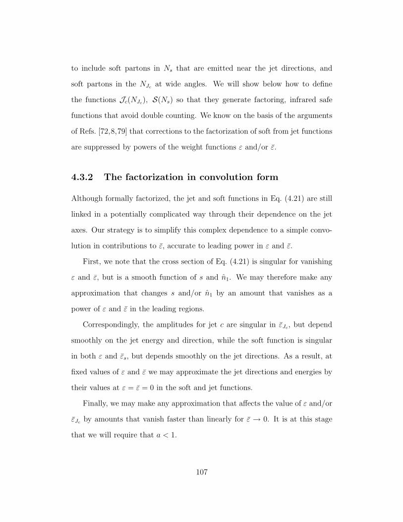
to include soft partons in Ns that are emitted near the jet directions, and
soft partons in the NJc at wide angles. We will show below how to define
the functions Jc(NJc), S(Ns) so that they generate factoring, infrared safe
functions that avoid double counting. We know on the basis of the arguments
of Refs. [72,8,79] that corrections to the factorization of soft from jet functions
are suppressed by powers of the weight functions ε and/or ε.
4.3.2 The factorization in convolution form
Although formally factorized, the jet and soft functions in Eq. (4.21) are still
linked in a potentially complicated way through their dependence on the jet
axes. Our strategy is to simplify this complex dependence to a simple convo-
lution in contributions to ε, accurate to leading power in ε and ε.
First, we note that the cross section of Eq. (4.21) is singular for vanishing
ε and ε, but is a smooth function of s and n1. We may therefore make any
approximation that changes s and/or n1 by an amount that vanishes as a
power of ε and ε in the leading regions.
Correspondingly, the amplitudes for jet c are singular in εJc, but depend
smoothly on the jet energy and direction, while the soft function is singular
in both ε and εs, but depends smoothly on the jet directions. As a result, at
fixed values of ε and ε we may approximate the jet directions and energies by
their values at ε = ε = 0 in the soft and jet functions.
Finally, we may make any approximation that affects the value of ε and/or
εJc by amounts that vanish faster than linearly for ε → 0. It is at this stage
that we will require that a < 1.
107

With these observations in mind, we enumerate the replacements and ap-
proximations by which we reduce Eq. (4.21), while retaining leading-power
accuracy.
1. To simplify the definitions of the jets in Eq. (4.21), we make the replace-
ments fNΩc
(NJc , a) → fc(NJc, a) with
fc(NJc, a) ≡ 1√s
∑
all ni∈NJc
kai,⊥ ω1−a
i (1 − ni · nc)1−a . (4.22)
The jet weight function fc(NJc, a) now depends only on particles asso-
ciated with NJc. The contribution to fc(NJc , a) from particles within
region Ωc, is exactly the same here as in the weight (4.3), but we now in-
clude particles in all other directions. In this way, the independent sums
over final states of the jet amplitudes will be naturally infrared safe. The
value of fc(NJc , a) differs from the value of fNΩc
(NJc , a), however, due to
radiation outside Ωc, as indicated by the new subscript. This radiation
is hence at wide angles to the jet axis. In the elastic limit (4.8), it is
also constrained to be soft. Double counting in contributions to the total
event shape, f(N, a), will be avoided by an appropriate definition of the
soft function below. The sums over states are still not yet fully indepen-
dent, however, because the jet directions nc still depend on the full final
state N .
2. Next, we turn our attention to the condition that fixes the jet direction
n1. Up to corrections in the orientation of n1 that vanish as powers of ε
108

and ε, we may neglect the dependence of n1 on Ns and NJ2 :
δ(n1 − n(N)) → δ(n1 − n(NJ1)) . (4.23)
In Appendix C.2, we show that this replacement also leaves the value of ε
unchanged, up to corrections that vanish as ε2−a. Thus, for a < 1, (4.23)
is acceptable to leading power. For a < 1, we can therefore identify the
direction of jet 1 with n1. These approximations simplify Eq. (4.21) by
eliminating the implicit dependence of the jet and soft weights on the
full final state. We may now treat n1 as an independent vector.
3. In the leading regions, particles that make up each final-state jet are
associated with states NJc, while Ns consists of soft particles only. In
the momentum conservation delta function, we can neglect the four-
momenta of lines in Ns, whose energies all vanish as ε, ε → 0:
δ4(pI − p(NJ2) − p(NJ1) − p(Ns)) → δ4(pI − pJ2 − pJ1). (4.24)
4. Because the cross section is a smooth function of the jet energies and
directions, we may also neglect the masses of the jets within the momen-
tum conservation delta function, as in Eq. (4.10). In this approximation,
109

we derive in the c.m.,
δ4(pI − pJ2 − pJ1) → δ(√
s − ω(NJ1) − ω(NJ2)) δ(|~pJ1| − |~pJ2|)1
|~pJ1|2× δ2(n1 + n2)
→ 2
sδ
(√s
2− ω(NJ1)
)
δ
(√s
2− ω(NJ2)
)
× δ2(n1 + n2) . (4.25)
Our jets are now back-to-back:
n2 → −n1 . (4.26)
Implementing these replacements and approximations for a < 1, we rewrite
the cross section Eq. (4.21) as
dσ(ε, ε, s, a)
dε dε dn1
=dσ0
dn1
H(s, n1, µ)
∫
dεs S(ε, εs, a, µ)
×2∏
c=1
∫
dεJc Jc(εJc, a, µ) δ(ε − εJ1 − εJ2 − εs) , (4.27)
with (as above) H = 1 + O(αs). Referring to the notation of Eqs. (4.21) and
(4.22), the functions S and Jc are:
S(ε, εs, a, µ) =∑
Ns
S(Ns, µ) δ(ε − f(Ns)) δ(εs − f(Ns, a)) (4.28)
Jc(εJc, a, µ) =2
s(2π)6
∑
NJc
Jc(NJc , µ) δ(εJc − fc(NJc, a)) δ
(√s
2− ω(NJc)
)
× δ2(n1 ± n(NJc)),
(4.29)
110

with the plus sign in the angular delta function for jet 2, and the minus for
jet 1. The weight functions for the jets are given by Eq. (4.22) and induce
dependence on the parameter a. We have introduced the factorization scale
µ, which we set equal to the renormalization scale.
We note that we must construct the soft functions S(Ns, µ) to cancel the
contributions of final-state particles from each of the Jc(NJc , µ) to the weight ε,
as well as the contributions of the jet functions to ε from soft radiation outside
their respective regions Ωc. Similarly, the jet amplitudes must be constructed
to include collinear enhancements only in their respective jet directions. Ex-
plicit constructions that satisfy these requirements will be specified in the
following subsections.
To disentangle the convolution in (4.27), we take Laplace moments with
respect to ε:
dσ(ε, ν, s, a)
dε dn1=
∫ ∞
0
dε e−ν ε dσ(ε, ε, a)
dε dε dn1
=dσ0
dn1H(s, n1, µ) S(ε, ν, a, µ)
2∏
c=1
Jc(ν, a, µ). (4.30)
Here and below unbarred quantities are the transforms in ε, and barred quan-
tities denote untransformed functions.
S(ε, ν, a, µ) =
∫ ∞
0
dεs e−ν εsS(ε, εs, a, µ), (4.31)
and similarly for the jet functions.
In the following subsections, we give explicit constructions for the functions
participating in the factorization formula (4.27), which satisfy the requirement
111
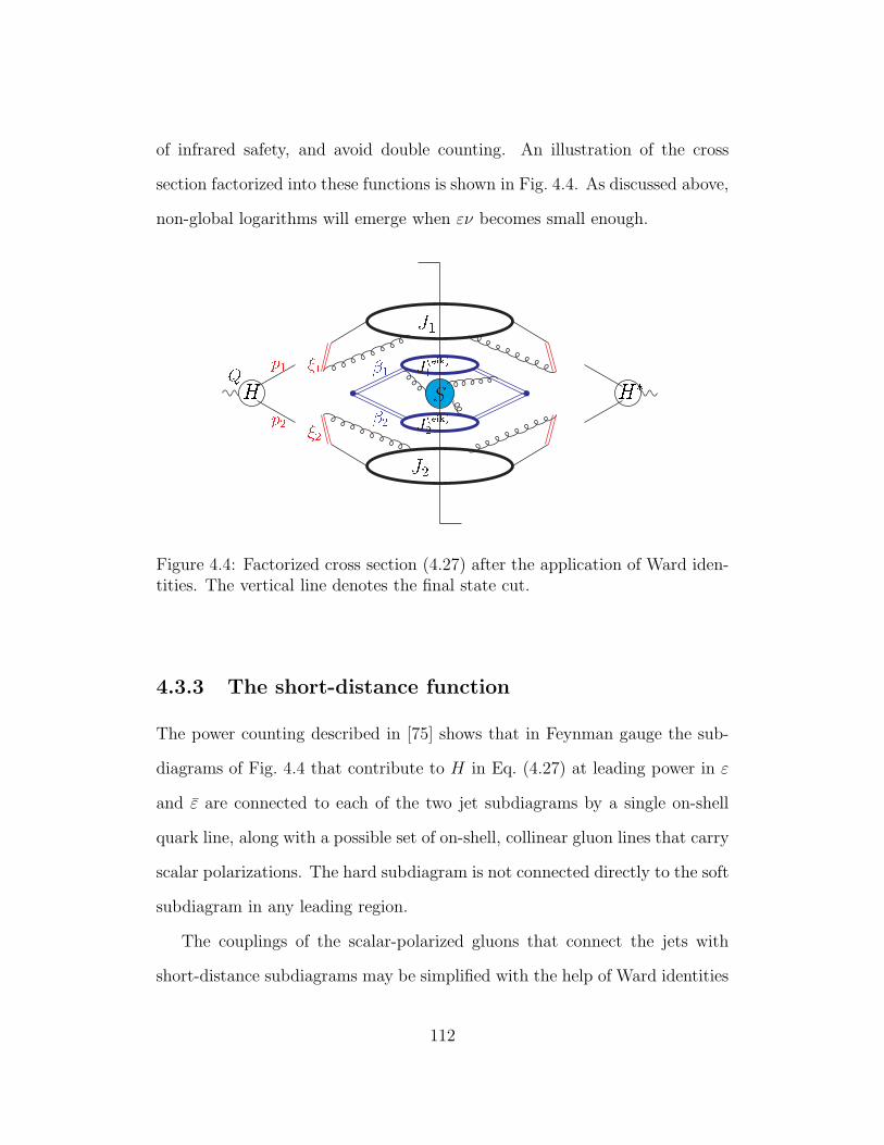
of infrared safety, and avoid double counting. An illustration of the cross
section factorized into these functions is shown in Fig. 4.4. As discussed above,
non-global logarithms will emerge when εν becomes small enough.
H HQ p1p2J1J2
12 S12 J (eik)1J (eik)2Figure 4.4: Factorized cross section (4.27) after the application of Ward iden-tities. The vertical line denotes the final state cut.
4.3.3 The short-distance function
The power counting described in [75] shows that in Feynman gauge the sub-
diagrams of Fig. 4.4 that contribute to H in Eq. (4.27) at leading power in ε
and ε are connected to each of the two jet subdiagrams by a single on-shell
quark line, along with a possible set of on-shell, collinear gluon lines that carry
scalar polarizations. The hard subdiagram is not connected directly to the soft
subdiagram in any leading region.
The couplings of the scalar-polarized gluons that connect the jets with
short-distance subdiagrams may be simplified with the help of Ward identities
112

(see, e. g. [8]). At each order of perturbation theory, the coupling of scalar-
polarized gluons from either jet to the short-distance function is equivalent
to their coupling to a path-ordered exponential of the gauge field, oriented in
any direction that is not collinear to the jet. Corrections are infrared safe,
and can be absorbed into the short-distance function. Let h(pJc , n1,A) rep-
resent the set of all short-distance contributions to diagrams that couple any
number of scalar-polarized gluons to the jets, in the amplitude for the produc-
tion of any final state. The argument A stands for the fields that create the
scalar-polarized gluons linking the short-distance function to the jets. On a
diagram-by-diagram basis, h depends on the momentum of each of the scalar-
polarized gluons. After the sum over all diagrams, however, we can make the
replacement:
h(pJc , n1,A(q,q)) → Φ(q)ξ2
(0,−∞; 0) h2(pJc, n1, ξc) Φ(q)ξ1
(0,−∞; 0) , (4.32)
where h2 is a short-distance function that depends only on the total momenta
pJ1 and pJ2 . It also depends on vectors ξc that characterize the path-ordered
exponentials Φ(0,−∞; 0):
Φ(f)ξc
(0,−∞; 0) = Pe−ig∫ 0−∞
dλ ξc·A(f)(λξc) , (4.33)
where the superscript (f) indicates that the vector potential takes values in
representation f, in our case the representation of a quark or antiquark. These
operators will be associated with gauge-invariant definitions of the jet functions
below. To avoid spurious collinear singularities, we choose the vectors ξc,
113

c = 1, 2, off the light cone. In the full cross section (4.30) the ξc-dependence
cancels, of course.
The dimensionless short-distance function H = |h2|2 in Eq. (4.27) depends
on√
s and pJc · ξc, but not on any variable that vanishes with ε and ε:
H(pJc , ξc, n1, µ) = H
(√s
µ,pJc · ξc
µ, n1, αs(µ)
)
, (4.34)
where
ξc ≡ ξc/√
|ξ2c | . (4.35)
Here we have observed that each diagram is independent of the overall scale
of the eikonal vector ξµc .
4.3.4 The jet functions
The jet functions and the soft functions in Eq. (4.27) can be defined in terms
of specific matrix elements, which absorb the relevant contributions to leading
regions in the cross section, and which are infrared safe. Their perturbative
expansions specify the functions S and Jc of Eq. (4.29). We begin with our
definition of the jet functions.
The jet functions, which absorb enhancements collinear to the two outgoing
particles produced in the primary hard scattering, can be defined in terms
of matrix elements in a manner reminiscent of parton distribution or decay
114

functions [77]. To be specific, we consider the quark jet function:
J ′µc (εJc, a, µ) =
2
s
(2π)6
NC
∑
NJc
Tr[
γµ⟨
0∣
∣
∣Φ
(q)ξc
†(0,−∞; 0)q(0)∣
∣
∣NJc
⟩
×⟨
NJc
∣
∣
∣q(0)Φ
(q)ξc
(0,−∞; 0)∣
∣
∣0⟩]
× δ(εJc − fc(NJc , a)) δ
(√s
2− ω(NJc)
)
× δ2(nc − n(NJc)) , (4.36)
where NC is the number of colors, and where nc denotes the direction of
the momentum of jet c, Eq. (4.29), with n2 = −n1. q is the quark field,
Φ(q)ξc
(0,−∞; 0) a path-ordered exponential in the notation of (4.33), and the
trace is taken over color and Dirac indices. We have chosen the normalization
so that the jet functions J ′µ in (4.36) are dimensionless and begin at lowest
order with
J ′µc(0)(εJc, a, µ) = βµ
c δ(εJc) , (4.37)
with βµc the lightlike velocities corresponding to the jet momenta in Eq. (4.10):
βµ1 = δµ+ , βµ
2 = δµ− . (4.38)
The scalar jet functions of Eq. (4.29) are now obtained by projecting out the
component of J ′cµ in the jet direction:
Jc(εJc , a, µ) = βc · J ′c(εJc, a, µ) = δ(εJc) + O(αs) , (4.39)
115
where β1 = β2, β2 = β1 are the lightlike vectors in the directions opposite to
β1 and β2, respectively. By construction, the Jc are linear in βc.
To resum the jet functions in the variables εJc , it is convenient to reexpress
the weight functions (4.22) in combinations of light-cone momentum compo-
nents that are invariant under boosts in the x3 direction,
f1 (NJ1, a) =1
s1−a/2
∑
ni∈NJ1
kai,⊥(
2p+J1
k−i
)1−a,
f2 (NJ2, a) =1
s1−a/2
∑
ni∈NJ2
kai,⊥(
2p−J2k+
i
)1−a. (4.40)
Here we have used the relation√
s/2 = ωJc, valid for both jets in the c.m. At
the same time, we make the identification,
1
sδ
(√s
2− ω(NJc)
)
δ2(nc − n(NJc)) =1
4δ3 (~pJc − ~p(NJc)) , (4.41)
which again holds in the c.m. frame. The spatial components of each pJc are
thus fixed. Given that we are at small εJc, the jet functions may be thought
of as functions of the light-like jet momenta pµJc
of Eq. (4.10) and of εJc.
Because the vector jet function is constructed to be dimensionless, J ′µc in Eq.
(4.36) is proportional to βc rather than pJc . Otherwise, it is free of explicit
βc-dependence.
The jet functions can now be written in terms of boost-invariant arguments,
116

homogeneous of degree zero in ξc:
Jc (εJc , a, µ) = βc µ
[
βµc J (1)
c
(
pJc · ξc
µ, εJc
√s
µ
( √s
2pJc · ξc
)1−a
, a, αs(µ)
)
+2 ξµ
c βc · ξc
|ξc|2J (2)
c
(
pJc · ξc
µ, εJc
√s
µ
( √s
2pJc · ξc
)1−a
, a, αs(µ)
)]
,
(4.42)
where J (1) and J (2) are independent functions, and where we have suppressed
possible dependence on ξc,⊥. For jet c, the weight εJc is fixed by δ(εJc −
fc(NJc , a)), where on the right-hand side of the expression for the weight
(4.40), the sum over each particle’s momentum involves the overall factor
(2p±Jc/√
s)1−a. After integration over final states at fixed εJc, the jet can
thus depend on the vector pµJc
. At the same time, it is easy to see from
the definition of the weight that pµJc
can only appear in the combination
(1/εJc
√s)1/(1−a) (2pµ
Jc/√
s). This vector can combine with ξc to form an in-
variant, and all ξc-dependence comes about in this way.
Expression (4.42) can be further simplified by noting that
2 βc · ξc βc · ξc = ξ2c + ξ2
c,⊥ . (4.43)
Choosing ξc,⊥ = 0, we find a single combination,
Jc (εJc, a, µ) = Jc
(
pJc · ξc
µ, εJc
√s
µ(ζc)
1−a , a, αs(µ)
)
, (4.44)
117

where, in the notation of Eq. (4.42), Jc = J(1)c + J
(2)c , and we have defined
ζc ≡√
s
2pJc · ξc
. (4.45)
In these terms, the Laplace moments of the jet function inherit dependence
on the moment variable ν through
Jc (ν, a, µ) =
∫ ∞
0
dεJc e−νεJc Jc (εJc, a, µ)
≡ Jc
(
pJc · ξc
µ,
√s
µν(ζc)
1−a , a, αs(µ)
)
, (4.46)
where the unbarred and barred quantities denote transformed and untrans-
formed functions, respectively. We have constructed the jet functions to be
independent of ε, since the radiation into Ω is at wide angles from the jet axes
and can therefore be completely factored from the collinear radiation. This
radiation at wide angles is contained in the soft function, which will be defined
below in a manner that avoids double counting in the cross section.
4.3.5 The soft function
Given the definitions for the jet functions in the previous subsection, and the
factorization (4.27), we may in principle calculate the soft function S order by
order in perturbation theory. We can derive a more explicit definition of the
soft function, however, by relating it to an eikonal analog of Eq. (4.27).
As reviewed in Refs. [66, 8], soft radiation at wide angles from the jets
decouples from the collinear lines within the jet. As a result, to compute
amplitudes for wide-angle radiation, the jets may be replaced by nonabelian
118
phases, or Wilson lines. We therefore construct a dimensionless quantity, σ(eik),
in which gluons are radiated by path-ordered exponentials Φ, which mimic the
color flow of outgoing quarks,
Φ(f)βc
(∞, 0; x) = Pe−ig∫
∞
0dλβc·A(f)(λβc+x), (4.47)
with βc a light-like velocity in either of the jet directions. For the two-jet cross
section at measured ε and εeik, we define
σ(eik) (ε, εeik, a, µ) ≡ 1
NC
∑
Neik
⟨
0∣
∣
∣Φ
(q)β2
†(∞, 0; 0)Φ(q)β1
†(∞, 0; 0)∣
∣
∣Neik
⟩
×⟨
Neik
∣
∣
∣Φ
(q)β1
(∞, 0; 0)Φ(q)β2
(∞, 0; 0)∣
∣
∣0⟩
× δ (ε − f(Neik)) δ(
εeik − f(Neik, a))
= δ(ε) δ(εeik) + O(αs) . (4.48)
The sum is over all final states Neik in the eikonal cross section. The renormal-
ization scale in this cross section, which will also serve as a factorization scale,
is denoted µ. Here the event shape function εeik is defined by f(Neik, a) as in
Eqs. (4.3) and (4.4), distinguishing between the hemispheres around the jets.
As usual, NC is the number of colors, and a trace over color is understood.
The eikonal cross section (4.48) models the soft radiation away from the
jets, including the radiation into Ω, accurately. It also contains enhancements
for configurations collinear to the jets, which, however, are already taken into
account by the partonic jet functions in (4.27). Indeed, (4.48) does not repro-
duce the partonic cross section accurately for collinear radiation. It is also easy
to verify at lowest order that even at fixed εeik the eikonal cross section (4.48)
119

is ultraviolet divergent in dimensional regularization, unless we also impose a
cutoff on the energy of real gluon emission collinear to β1 or β2.
The construction of the soft function S from σ(eik) is nevertheless possi-
ble because the eikonal cross section (4.48) factorizes in the same manner as
the cross section itself, into eikonal jet functions and a soft function. The
essential point [65] is that the soft function in the factorized eikonal cross
section is the same as in the original cross section (4.27). The eikonal jets or-
ganize all collinear enhancements in (4.48), including the spurious ultraviolet
divergences. These eikonal jet functions are defined analogously to their par-
tonic counterparts, Eq. (4.36), but now with ordered exponentials replacing
the quark fields,
J (eik)c (εc, a, µ) ≡ 1
NC
∑
N(eik)c
⟨
0∣
∣
∣Φ
(fc)ξc
†(0,−∞; 0)Φ(fc)βc
†(∞, 0; 0)∣
∣
∣N (eik)
c
⟩
×⟨
N (eik)c
∣
∣
∣Φ
(fc)βc
(∞, 0; 0)Φ(fc)ξc
(0,−∞; 0)∣
∣
∣0⟩
× δ(
εc − fc(N(eik)c , a)
)
= δ(εc) + O(αs) , (4.49)
where fc is a quark or antiquark, and where the trace over color is understood.
The weight functions are given as above, by Eq. (4.22), with the sum over
particles in all directions.
In terms of the eikonal jets, the eikonal cross section (4.48) factorizes as
σ(eik) (ε, εeik, a, µ) ≡∫
dεs S (ε, εs, a, µ)
2∏
c=1
∫
dεc J (eik)c (εc, a, µ)
× δ (εeik − εs − ε1 − ε2) , (4.50)
120
where we pick the factorization scale equal to the renormalization scale µ. As
for the full cross section, the convolution in (4.50) is simplified by a Laplace
transformation (4.46) with respect to εeik, which allows us to solve for the soft
function as
S (ε, ν, a, µ) =σ(eik) (ε, ν, a, µ)2∏
c=1
J(eik)c (ν, a, µ)
= δ(ε) + O(αs) . (4.51)
In this ratio, collinear logarithms in ν and the unphysical ultraviolet diver-
gences and their associated cutoff dependence cancel between the eikonal cross
section and the eikonal jets, leaving a soft function that is entirely free of
collinear enhancements. The soft function retains ν-dependence through soft
emission, which is also restricted by the weight function ε. In addition, be-
cause soft radiation within the eikonal jets can be factored from its collinear
radiation, just as in the partonic jets, all logarithms in ν associated with wide-
angle radiation are identical between the partonic and eikonal jets, and factor
from logarithmic corrections associated with collinear radiation in both cases.
As a result, the inverse eikonal jet functions cancel contributions from the
wide-angle soft radiation of the partonic jets in the transformed cross section
(4.30).
Given the definition of the energy flow weight function f , Eq. (4.5), the
soft function is not boost invariant. In addition, because it is free of collinear
logs, it can have at most a single logarithm per loop. Its dependence on ε
is therefore only through ratios of the dimensional quantities ε√
s with the
renormalization (factorization) scale.
121

As in the case of the partonic jets, Eq. (4.46), we need to identify the vari-
able through which ν appears in the soft function. We note that dependence
on the velocity vectors βc and the factorization vectors ξc must be scale invari-
ant in each, since they arise only from eikonal lines and vertices. The eikonal
jet functions cannot depend explicitly on the scale-less, lightlike eikonal veloc-
ities βc, and σ(eik) is independent of the ξc. Dependence on the factorization
vectors ξc enters only through the weight functions, (4.40) for the eikonal jets,
in a manner analogous to the case of the partonic jets. This results in a de-
pendence on (ζc)1−a, as above, with ζc defined in Eq. (4.45). In summary, we
may characterize the arguments of the soft function in transform space as
S (ε, ν, a, µ) = S
(
ε√
s
µ, εν,
√s
µν(ζc)
1−a , a, αs(µ)
)
. (4.52)
4.4 Resummation
We may summarize the results of the previous section by rewriting the trans-
form of the factorized cross section (4.30) in terms of the hard, jet and soft
functions identified above, which depend on the kinematic variables and the
moment ν according to Eqs. (4.34), (4.46) and (4.52) respectively,
dσ (ε, ν, s, a)
dε dn1=
dσ0
dn1H
(√s
µ,pJc · ξc
µ, n1, αs(µ)
)
×2∏
c=1
Jc
(
pJc · ξc
µ,
√s
µν(ζc)
1−a, a, αs(µ)
)
× S
(
ε√
s
µ, εν,
√s
µν(ζc)
1−a , a, αs(µ)
)
. (4.53)
122

The natural scale for the strong coupling in the short-distance function H is
√s/2. Setting µ =
√s/2, however, introduces large logarithms of ε in the
soft function and large logarithms of ν in both the soft and jet functions. The
purpose of this section is to control these logarithms by the identification and
solution of renormalization group and evolution equations.
The information necessary to perform the resummations is already present
in the factorization (4.53). The cross section itself is independent of the fac-
torization scale
µd
dµ
dσ (ε, ν, s, a)
dεdn1
= 0 , (4.54)
and of the choice of the eikonal directions, ξc, used in the factorization,
∂
∂ ln(
pJc · ξc
)
dσ (ε, ν, s, a)
dεdn1= 0 . (4.55)
The arguments of this section closely follow the analysis of Ref. [80]. We will
see that the dependence of jet and soft functions on the parameter a that
characterizes the event shapes (3) is reflected in the resummed correlations,
so that the relationship between correlations with different values of a is both
calculable and nontrivial.
4.4.1 Energy flow
As a first step, we use the renormalization group equation (4.54) to organize
dependence on the energy flow variable ε. Applying Eq. (4.54) to the factorized
correlation (4.53), we derive the following consistency conditions, which are
123
themselves renormalization group equations:
µd
dµln S
(
ε√
s
µ, εν,
√s
µν(ζc)
1−a, a, αs(µ)
)
= −γs (αs(µ)) , (4.56)
µd
dµln Jc
(
pJc · ξc
µ,
√s
µν(ζc)
1−a, a, αs(µ)
)
= −γJc (αs(µ)) , (4.57)
µd
dµln H
(√s
µ,pJc · ξc
µ, n1, αs(µ)
)
= γs (αs(µ)) +
2∑
c=1
γJc (αs(µ)) .
(4.58)
The anomalous dimensions γd, d = s, Jc can depend only on variables held
in common between at least two of the functions. Because each function is
infrared safe, while ultraviolet divergences are present only in virtual diagrams,
the anomalous dimensions cannot depend on the parameters ν, ε or a. This
leaves as arguments of the γd only the coupling αs(µ), which we exhibit, and
ζc, which we suppress for now.
Solving Eqs. (4.56) and (4.57) we find
S
(
ε√
s
µ, εν,
√s
µν(ζc)
1−a , a, αs(µ)
)
= S
(
ε√
s
µ0, εν,
√s
µ0ν(ζc)
1−a , a, αs(µ0)
)
× e−
µ∫
µ0
dλλ
γs(αs(λ))
, (4.59)
Jc
(
pJc · ξc
µ,
√s
µν(ζc)
1−a , a, αs(µ)
)
= Jc
(
pJc · ξc
µ0
,
√s
µ0ν(ζc)
1−a , a, αs(µ0)
)
× e−
µ∫
µ0
dλλ
γJc(αs(λ))
, (4.60)
for the soft and jet functions. As suggested above, we will eventually pick
µ ∼ √s to avoid large logs in H . Using these expressions in Eq. (4.53) we
124
can avoid logarithms of ε or ν in the soft function, by evolving from µ0 = ε√
s
to the factorization scale µ ∼ √s. No choice of µ0, however, controls all
logarithms of ν in the jet functions. Leaving µ0 free, we find for the cross
section (4.53) the intermediate result
dσ (ε, ν, s, a)
dε dn1=
dσ0
dn1H
(√s
µ,pJc · ξc
µ, n1, αs(µ)
)
× S(
1, εν, (ζc)1−a, a, αs(ε
√s))
exp
−µ∫
ε√
s
dλ
λγs (αs(λ))
(4.61)
× Jc
(
pJc · ξc
µ0
,
√s
µ0ν(ζc)
1−a , a, αs(µ0)
)
exp
−µ∫
µ0
dλ
λγJc (αs(λ))
.
We have avoided introducing logarithms of ε into the jet functions, which
originally only depend on ν, by evolving the soft and the jet functions inde-
pendently. The choice of µ0 = ε√
s or√
s/ν for the soft function is to some
extent a matter of convenience, since the two choices differ by logarithms of εν.
In general, if we choose µ0 =√
s/ν, logarithms of εν will appear multiplied by
coefficients that reflect the size of region Ω. An example is Eq. (4.15) above.
When Ω has a small angular size, µ0 =√
s/ν is generally the more natural
choice, since then logarithms in εν will enter with small weights. In contrast,
when Ω grows to cover most angular directions, as in the study of rapidity
gaps [82], it is more natural to choose µ0 = ε√
s.
125

4.4.2 Event shape transform
The remaining unorganized “large” logarithms in (4.61), are in the jet func-
tions, which we will resum by using the consistency equation (4.55). The
requirement that the cross section be independent of pJc · ξc implies that the
jet, soft and hard functions obey equations analogous to (4.56)–(4.58), again
in terms of the variables that they hold in common [80]. The same results may
be derived following the method of Collins and Soper [72], by defining the jets
in an axial gauge, and then studying their variations under boosts.
For our purposes, only the equation satisfied by the jet functions [72,80] is
necessary,
∂
∂ ln(
pJc · ξc
) ln Jc
(
pJc · ξc
µ,
√s
µν(ζc)
1−a, a, αs(µ)
)
= Kc
(√s
µ ν(ζc)
1−a, a, αs(µ)
)
+ Gc
(
pJc · ξc
µ, αs(µ)
)
.(4.62)
The functions Kc and Gc compensate the ξc-dependence of the soft and hard
functions, respectively, which determines the kinematic variables upon which
they may depend. In particular, notice the combination of ν- and ξc-dependence
required by the arguments of the jet function, Eq. (4.46).
Since the definition of our jet functions (4.36) is gauge invariant, we can
derive the kernels Kc and Gc by an explicit computation of ∂ Jc/∂ ln(
pJc · ξc
)
in any gauge. The multiplicative renormalizability of the jet function, Eq.
(4.57), with an anomalous dimension that is independent of pJc · ξc ensures
that the right-hand side of Eq. (4.62) is a renormalization-group invariant.
126

Thus, Kc + Gc are renormalized additively, and satisfy [72]
µd
dµKc
(√s
µ ν(ζc)
1−a , a, αs(µ)
)
= −γKc (αs(µ)) ,
µd
dµGc
(
pJc · ξc
µ, αs(µ)
)
= γKc (αs(µ)) . (4.63)
Since Gc and hence γKc , may be computed from virtual diagrams, they do not
depend on a, and γKc is the universal Sudakov anomalous dimension [72, 83].
With the help of these evolution equations, the terms Kc and Gc in Eq.
(4.62) can be reexpressed as [84]
Kc
(√s
µ ν(ζc)
1−a , a, αs(µ)
)
+ Gc
(
pJc · ξc
µ, αs(µ)
)
= Kc
(
1
c1, a, αs
(
c1
√s
ν(ζc)
1−a
))
+ Gc
(
1
c2, αs
(
c2 pJc · ξc
)
)
−c2 pJc ·ξc∫
c1√
s (ζc)1−a/ν
dλ′
λ′ γKc (αs (λ′))
= −B′c
(
c1, c2, a, αs
(
c2 pJc · ξc
))
− 2
c2 pJc ·ξc∫
c1√
s (ζc)1−a/ν
dλ′
λ′ A′c (c1, a, αs (λ′)) ,
(4.64)
where in the second equality we have shifted the argument of the running
127
coupling in Kc, and have introduced the notation
B′c (c1, c2, a, αs (µ)) ≡ −Kc
(
1
c1, a, αs (µ)
)
− Gc
(
1
c2, αs (µ)
)
,
2A′c (c1, a, αs (µ)) ≡ γKc (αs(µ)) + β(g(µ))
∂
∂g(µ)Kc
(
1
c1, a, αs(µ)
)
.
(4.65)
The primes on the functions A′c and B′
c are to distinguish these anomalous
dimensions from their somewhat more familiar versions given below.
The solution to Eq. (4.62) with µ = µ0 is
Jc
(
pJc · ξc
µ0
,
√s
µ0ν(ζc)
1−a , a, αs(µ0)
)
= Jc
( √s
2 ζ0 µ0
,
√s
µ0ν(ζ0)
1−a , a, αs(µ0)
)
× exp
−pJc ·ξc∫
√s/(2ζ0)
dλ
λ
B′c (c1, c2, a, αs (c2λ)) + 2
c2 λ∫
c1s1−a/2
ν(2 λ)1−a
dλ′
λ′ A′c (c1, a, αs (λ′))
,
(4.66)
where we evolve from√
s/(2 ζ0) to pJc · ξc =√
s/(2 ζc) (see Eq. (4.45)) with
ζ0 =(ν
2
)1/(2−a)
. (4.67)
After combining Eqs. (4.60) and (4.66), the choice µ0 =√
s/(2ζ0) =√
sν
(ζ0)1−a
128

allows us to control all large logarithms in the jet functions simultaneously:
Jc
(
pJc · ξc
µ,
√s
µν(ζc)
1−a, a, αs(µ)
)
= Jc
(
1, 1, a, αs
(√s
2 ζ0
))
× exp
−µ∫
√s/(2ζ0)
dλ
λγJc (αs(λ))
× exp
−pJc ·ξc∫
√s/(2 ζ0)
dλ
λ
B′c (c1, c2, a, αs (c2λ)) + 2
c2 λ∫
c1s1−a/2
ν(2 λ)1−a
dλ′
λ′ A′c (c1, a, αs (λ′))
.
(4.68)
As observed above, we treat a as a fixed parameter, with |a| small compared
to ln (1/ε) and ln ν.
129

4.4.3 The resummed correlation
Using Eq. (4.68) in (4.61), and setting µ =√
s/2, we find a fully resummed
form for the correlation,
dσ (ε, ν, s, a)
dε dn1=
dσ0
dn1H
(
2 pJc · ξc√s
, n1, αs
(√s
2
)
)
×S(
1, εν, (ζc)1−a, a, αs(ε
√s))
exp
−
√s/2∫
ε√
s
dλ
λγs (αs(λ))
×2∏
c=1
Jc
(
1, 1, a, αs
(√s
2 ζ0
))
exp
−
√s/2∫
√s/(2 ζ0)
dλ
λγJc (αs(λ))
× exp
−pJc ·ξc∫
√s/(2 ζ0)
dλ
λ
B′c (c1, c2, a, αs (c2λ)) + 2
c2 λ∫
c1s1−a/2
ν(2 λ)1−a
dλ′
λ′ A′c (c1, a, αs (λ′))
.
(4.69)
Alternatively, we can combine all jet-related exponents in Eq. (4.69) in
the correlation. As we will verify below in Section 4.5.2, the cross section is
independent of the choice of ξc. As a result, we can choose
pJc · ξc =
√s
2. (4.70)
130

This choice allows us to combine γJc and B′c in Eq. (4.69),
dσ (ε, ν, s, a)
dε dn1=
dσ0
dn1H
(
1, n1, αs
(√s
2
))
×S(
1, εν, 1, a, αs(ε√
s))
exp
−
√s/2∫
ε√
s
dλ
λγs (αs(λ))
2∏
c=1
Jc
(
1, 1, a, αs
(√s
2 ζ0
))
× exp
−
√s/2∫
√s/(2 ζ0)
dλ
λ[γJc (αs(λ)) + B′
c (c1, c2, a, αs (c2λ))
+2
c2 λ∫
c1s1−a/2
ν(2 λ)1−a
dλ′
λ′ A′c (c1, a, αs (λ′))
,
(4.71)
with ζ0 given by Eq. (4.67).
In Eqs. (4.69) and (4.71), the energy flow ε appears at the level of one
logarithm per loop, in S, in the first exponent. Leading logarithms of ε are
therefore resummed by knowledge of γ(1)s , the one-loop soft anomalous dimen-
sion, where we employ the standard notation,
γs(αs) =
∞∑
n=0
γ(n)s
(αs
π
)n
(4.72)
for any expansion in αs. At the same time, ν appears in up to two logarithms
per loop, characteristic of conventional Sudakov resummation. To control
ν-dependence at the same level as ε-dependence, it is natural to work to next-
to-leading logarithm in ν, by which we mean the level αks lnk ν in the exponent.
As usual, this requires one loop in B′c and γJc, and two loops in the Sudakov
131

anomalous dimension A′c, Eq. (4.65). These functions are straightforward to
calculate from their definitions given in the previous sections. Only the soft
function S in Eqs. (4.69) and (4.71) contains information on the geometry of
Ω. The exponents are partially process-dependent, but geometry-independent.
In Section 4.5, we will derive explicit expressions for these quantities, suitable
for resummation to leading logarithm in ε and next-to-leading logarithm in ν.
4.4.4 The inclusive event shape
It is also of interest to consider the cross section for e+e−-annihilation into
two jets without fixing the energy of radiation into Ω, but with the final state
radiation into all of phase space weighted according to Eq. (4.4), schematically
e+ + e− → J1(pJ1, fΩ1) + J2(pJ2 , fΩ2
) , (4.73)
where Ω1 and Ω2 cover the entire sphere. This cross section can be factorized
and resummed in a completely analogous manner. The final state is a convo-
lution in the contributions of the jet and soft functions to ε as in Eq. (4.27),
but with no separate restriction on energy flow into Ω. All particles contribute
to the event shape. We obtain an expression very analogous to Eq. (4.69) for
this inclusive event shape in transform space, which can be written in terms
of the same jet functions as before, and a new function S incl for soft radiation
132

as:
dσincl (ν, s, a)
dn1=
dσ0
dn1H
(
2pJc · ξc√s
, n1, αs(√
s/2)
)
× S incl
(
(ζc)1−a, a, αs
(√s
ν
))
exp
−
√s/2∫
√s/ν
dλ
λγs (αs(λ))
×2∏
c=1
Jc
(
1, 1, a, αs
(√s
2 ζ0
))
exp
−
√s/2∫
√s/(2 ζ0)
dλ
λγJc (αs(λ))
× exp
−pJc ·ξc∫
√s/(2 ζ0)
dλ
λ
B′c (c1, c2, a, αs (c2λ)) + 2
c2 λ∫
c1s1−a/2
ν(2 λ)1−a
dλ′
λ′ A′c (c1, a, αs (λ′))
.
(4.74)
Here the soft function S incl = 1 + O(αs). The double-logarithmic dependence
of the shape transform is identical to our resummed correlation, Eq. (4.69).
We will show below, in Sec. 4.5.3, that Eq. (4.74) coincides at NLL with the
known result for the thrust [57] when we choose a = 0.
4.5 Results at NLL
4.5.1 Lowest order functions and anomalous dimensions
In this section, we describe the low-order calculations and results that provide
explicit expressions for the resummed shape/flow correlations and inclusive
event shape distributions at next-to-leading logarithm in ν and leading log-
arithm in ε (we refer to this level collectively as NLL below). We go on to
133

verify that for the case a = 0 we rederive the known result for the resummed
thrust at NLL, and we exhibit the expressions for the correlation that we will
evaluate in Sec. 4.6.
The soft function
The one-loop soft anomalous dimension is readily calculated in Feynman gauge
from the combination of virtual diagrams in σ(eik), Eq. (4.48), and J (eik), Eq.
(4.49), in Eq. (4.51). The calculation and the result are equivalent to those of
Ref. [65], where the soft function was formulated in axial gauge,
γ(1)s = −2 CF
[
2∑
c=1
ln(
βc · ξc
)
− ln
(
β1 · β2
2
)
− 1
]
. (4.75)
The first, ξc-dependent logarithmic term is associated with the eikonal jets,
while the second is a finite remainder from the combination of σ(eik) and J (eik)
in (4.51). Whenever ξc,⊥ = 0, the logarithmic terms cancel identically, leaving
only the final term, which comes from the ξc eikonal self-energy diagrams in
the eikonal jet functions.
The soft function is normalized to S(0)(ε) = δ(ε) as can be seen from (4.51).
For non-zero ε, dσ/dε is given at lowest order by
S(1) (ε 6= 0, Ω) = CF1
ε
∫
Ω
dPS21
2π
β1 · β2
β1 · k β2 · k, (4.76)
where PS2 denotes the two-dimensional angular phase space to be integrated
over region Ω, and k ≡ k/ωk. We emphasize again that the soft function
contains the only geometry-dependence of the cross section. Also, S(1) for
134

ε 6= 0 is independent of ν and a.
As an example, consider a cone with opening angle 2δ, centered at angle
α from jet 1. In this case, the lowest-order soft function is given by
S(1) (ε 6= 0, α, δ) = CF1
εln
(
1 − cos2 α
cos2 α − cos2 δ
)
. (4.77)
Similarly, we may choose Ω as a ring extending angle δ1 to the right and δ2 to
the left of the plane perpendicular to the jet directions in the center-of-mass.
In this case, we obtain
S(1) (ε 6= 0, δ1, δ2) = CF1
εln
(
(1 + sin δ1)
(1 − sin δ1)
(1 + sin δ2)
(1 − sin δ2)
)
= CF2
ε∆η , (4.78)
with ∆η the rapidity spanned by the ring. For a ring centered around the
center-of-mass (δ1 = δ2 = δ) the angular integral reduces to the form that we
encountered in the example of Sec. 4.2.3, and that we will use in our numerical
examples of Sec. 4.6, with ∆η given by Eq. (4.14).
The jet functions
Recall from Eq. (4.39) that the lowest-order jet function is given by J(0)c = 1.
The anomalous dimensions of the jet functions are found to be
γ(1)Jc
= −3
2CF , (4.79)
the same for each of the jets. The jet anomalous dimensions are process-
independent, but of course flavor-dependent. The same anomalous dimensions
for final-state quark jets appear in three- and higher-jet cross sections.
135
The K-G-decomposition
The anomalous dimension for the K-G-decomposition is, as noted above, the
Sudakov anomalous dimension,
γ(1)Kc
= 2 CF , (4.80)
γ(2)Kc
= K CF , (4.81)
also independent of the jet-direction. The well-known coefficient K (not to be
confused with the functions Kc) is given by [85]
K =
(
67
18− π2
6
)
CA − 10
9TF Nf , (4.82)
with the normalization TF = 1/2 and Nf the number of quark flavors.
Kc and Gc, the functions that describe the evolution of the jet functions
in Eq. (4.62), are given at one loop by
K(1)c
(
s1−a/2
µν
(
2pJc · ξc
)a−1
, a
)
= −CF ln
(
e2γE−(1−a) µ2ν2
s2−a
(
2pJc · ξc
)2(1−a))
,
G(1)c
(
pJc · ξc
µ
)
= −CF ln
e−1
(
2 pJc · ξc
)2
µ2
. (4.83)
Evolving them to the values of µ with which they appear in the functions A′c
and B′c, Eq. (4.65), they become
K(1)c
(
1
c1
, a
)
= −CF ln(
e2γE−(1−a)c21
)
, (4.84)
G(1)c
(
1
c2
)
= −CF ln
(
e−1 4
c22
)
. (4.85)
136

Recall that Gc is computed from virtual diagrams only, and thus does not
depend on the weight function. It therefore agrees with the result found in [72].
The soft-gluon contribution, Kc, which involves real gluon diagrams, does
depend on the cross section being resummed.
With the definitions (4.65) of A′c and B′
c we obtain
A′ (1)c = CF , (4.86)
A′ (2)c (c1, a) =
1
2CF
[
K +β0
2ln(
e2γE−1+ac21
)
]
, (4.87)
B′ (1)c (c1, c2, a) = 2CF ln
(
eγE−1+a/2 2 c1
c2
)
. (4.88)
Here β0 is the one-loop coefficient of the QCD beta-function, β0 = 13(11NC − 4TF Nf)
(β(g) = −g αs
4πβ0 + O(g3)).
The hard scattering, and the Born cross section
At NLL only the lowest-order hard scattering function contributes, which is
normalized to
H(0)(αs(√
s/2)) = 1 . (4.89)
At this order the hard function is independent of the eikonal vectors ξc, al-
though it acquires ξc-dependence at higher order through the factorization
described in Sec. 4.3.3. For completeness, we also give the electromagnetic
Born cross section dσ0
dn1, at fixed polar and azimuthal angle:
dσ0
dn1
= NC
(
∑
f
Q2f
)
α2em
4s
(
1 + cos2 θ)
, (4.90)
137

where θ is the c.m. polar angle of n1, e Qf is the charge of quark flavor f, and
αem = e2/(4π) is the fine structure constant.
4.5.2 Checking the ξc-dependence
It is instructive to verify how dependence on the eikonal vectors ξc cancels in
the exponents of the resummed cross section (4.69) at the accuracy at which
we work, single logarithms of ε, and single and double logarithms of ν. In
these exponents, ξc-dependence enters only through the combinations (βc · ξc)
and (pJc · ξc).
Let us introduce the following notation for the exponents in Eq. (4.69), to
which we will return below:
E1 ≡ −
√s/2∫
ε√
s
dλ
λγs (αs(λ)) −
2∑
c=1
√s/2∫
√s/(2 ζ0)
dλ
λγJc (αs(λ)) , (4.91)
E2 ≡ −2∑
c=1
pJc ·ξc∫
√s/(2 ζ0)
dλ
λ
B′c (c1, c2, a, αs (c2λ)) + 2
c2 λ∫
c1s1−a/2
ν(2 λ)1−a
dλ′
λ′ A′c (c1, a, αs (λ′))
.
(4.92)
At NLL, explicit ξc dependence is found only in γs, Eq. (4.75), for E1, and in
the upper limit of the λ integral of E2. We then find that
∂
∂ ln βc · ξc
(E1 + E2) = 2CF
√s/2∫
ε√
s
dλ
λ
αs(λ)
π− 2CF
∫ c2 pJc ·ξc
c1s1−a/2
ν(2pJc·ξc)1−a
dλ′
λ′αs(λ
′)
π+ NNLL .
(4.93)
138

Here the second term stems entirely from A′ (1), Eq. (4.86); other contribu-
tions of E2 are subleading. The ξc-dependence in the exponents begins only
at the level that we do not resum, at αs ln(1/εν), which is compensated by
corrections in S(εν, αs). The remaining contributions are of NNLL order, that
is, proportional to αks(√
s) lnk−1(
ν βc · ξc
)
, as may be verified by expanding
the running couplings. Thus, as required by the factorization procedure, the
relevant ξc-dependence cancels between the resummed soft and jet functions,
which give rise to the first and second integrals, respectively, in Eq. (4.93).
4.5.3 The inclusive event shape at NLL
We can simplify the differential event shape, Eq. (4.74), by absorbing the soft
anomalous dimension γs into the remaining terms. We will find a form that can
be compared directly to the classic NLL resummation for the thrust (a = 0).
This is done by rewriting the integral over the soft anomalous dimension as
∫
√s/2
√s/ν
dλ
λγs (αs(λ)) =
∫
√s/2
√s/[2(ν/2)1/(2−a)]
dλ
λγs (αs(λ))
+
∫
√s/[2(ν/2)1/(2−a)]
√s/ν
dλ
λγs (αs(λ)) =
∫
√s/2
√s/[2(ν/2)1/(2−a)]
dλ
λγs (αs(λ))
+(1 − a)
∫
√s/2
√s/[2(ν/2)1/(2−a)]
dλ
λγs
(
αs
(
s1−a/2
ν(2λ)1−a
))
= (2 − a)
∫
√s/2
√s/[2(ν/2)1/(2−a)]
dλ
λγs (αs(λ))
−(1 − a)
∫
√s/2
√s/[2(ν/2)1/(2−a)]
dλ
λ
∫ λ
s1−a/2/[ν(2λ)1−a ]
dλ′
λ′ β(g(λ′))∂
∂gγs (αs(λ
′)) .
(4.94)
139

In the first equality we split the λ integral so that the limits of the first term
match those of the B′c integral of Eq. (4.74). In the second equality we have
changed variables in the second term according to
λ →(
s1− a2
21−aνλ
)
11−a
, (4.95)
so that the limits of the second integral also match. In the third equality of
Eq. (4.94), we have reexpressed the running coupling at the old scale λ in
terms of the new scale. This is a generalization of the procedure of Ref. [86],
applied originally to the threshold-resummed Drell-Yan cross section [87].
Using Eq. (4.94), and identifying pJc · ξc with√
s/2 (Eq. (4.70)) in the
inclusive event shape distribution, Eq. (4.74), we can rewrite this distribution
at NLL as
dσincl (ν, s, a)
dn1=
dσ0
dn1
×2∏
c=1
exp
−
√s/2∫
√s/[2(ν/2)1/(2−a)]
dλ
λ[Bc (c1, c2, a, αs (λ))
+ 2
c2 λ∫
c1s1−a/2
ν(2 λ)1−a
dλ′
λ′ Ac (c1, a, αs (λ′))
,
(4.96)
140

where we have rearranged the contribution of γs as:
Ac (c1, a, αs (µ)) ≡ A′c (c1, a, αs (µ)) − 1
4(1 − a) β(g(µ))
∂
∂gγs (αs(µ)) ,
Bc (c1, c2, a, αs (µ)) ≡ γJc (αs(µ)) +(
1 − a
2
)
γs (αs(µ)) + B′c (c1, c2, a, αs (µ)) .
(4.97)
Next, we replace the lower limit of the λ′-integral by an explicit θ-function.
Then we exchange orders of integration, and change variables in the term con-
taining A from the dimensionful variable λ to the dimensionless combination
u =2λλ′
s. (4.98)
We find
dσincl (ν, s, a)
dn1=
dσ0
dn1
2∏
c=1
exp
−
√s/2∫
√s/[2(ν/2)1/(2−a)]
dλ
λBc (c1, c2, a, αs (λ))
×2∏
c=1
exp
−2
∫
√s
0
dλ′
λ′
∫ λ′/√
s
λ′2/s
du
uθ
(
c−11 ν
λ′au1−a
sa/2− 1
)
Ac (c1, a, αs (λ′))
.
(4.99)
Here, the θ-function vanishes for small λ′, and the remaining effects of re-
placing the lower boundary of the λ′ integral by 0 are next-to-next-to-leading
logarithmic.
A further change of variables allows us to write the NLL resummed event
shapes in a form familiar from the NLL resummed thrust. In the first line of
Eq. (4.99), we replace λ2 → us/4. In the second line we relabel λ′ →√
q2,
141
and exchange orders of integration. Finally, choosing
c1 = e−γE ,
c2 = 2, (4.100)
we find at NLL
dσincl (ν, s, a)
dn1=
dσ0
dn1
×2∏
c=1
exp
1∫
0
du
u
us∫
u2s
dq2
q2Ac
(
αs(q2))
(
e−u1−aν(q2/s)a/2
− 1
)
+1
2Bc (αs(us/4))
(
e−u(ν/2)2/(2−a)e−γE − 1)
]
,
(4.101)
and reproduce the well-known coefficients
A(1)c = CF , (4.102)
A(2)c =
1
2CFK, (4.103)
B(1)c = −3
2CF , (4.104)
independent of a. In Eq. (4.101), we have made use of the relation
e−x/y − 1 ≈ −θ(
x − y e−γE)
, (4.105)
which is valid at NLL in the logarithmic integrals. With these choices, when
a = 0 we reproduce the NLL resummed thrust cross section [57].
142

The choices of the ci in Eq. (4.100) cancel all purely soft NLL compo-
nents (γs and Kc). The remaining double logarithms stem from simultane-
ously soft and collinear radiation, and single logarithms arise from collinear
configurations only. At NLL, the cross section is determined by the anomalous
dimension Ac, which is the coefficient of the singular 1/[1 − x]+ term in the
nonsinglet evolution kernel [88], and the quark anomalous dimension. All radi-
ation in dijet events thus appears to be emitted coherently by the two jets [57].
This, however, is not necessarily true beyond next-to-leading logarithmic ac-
curacy for dijets, and is certainly not the case for multijet events [65]. Similar
considerations apply to the resummed correlation, Eq. (4.69).
4.5.4 Closed expressions
Given the explicit results above, the integrals in the exponents of the resummed
correlation, Eq. (4.69), may be easily performed in closed form. We give the
analytic results for the exponents of Eq. (4.69), as defined in Eqs. (4.91) and
(4.92). As in Eq. (4.70), we identify pJc · ξc with√
s/2.
eE1(a) =
(
αs(√
s/2)
αs(ε√
s)
)
4CFβ0
αs
( √s
2 ζ0
)
αs(√
s/2)
6CFβ0
, (4.106)
eE2(a) =
αs(c2
√s/2)
αs
(
c2√
s2 ζ0
)
4CFβ0
κ1(a)
αs
(
c1√
s2 ζ0
)
αs
(
c1√
sν
)
1a−1
4CFβ0
κ2(a)
×
αs(c2
√s/2)
αs
(
c1√
s2 ζ0
)
12−a
8CFβ0
ln(ν/2)
,
(4.107)
143

with
κ1(a) = ln
(
4
c22e
)
+4π
β0
[
αs
(
c2
√s
2 ζ0
)]−1
− 2K
β0
− β1
2β20
ln
(
(
β0
4πe
)2
αs
(
c2
√s
2
)
αs
(
c2
√s
2 ζ0
)
)
,
(4.108)
κ2(a) = (1 − a − 2γE) +4π
β0
[
αs
(√s
ν
)]−1
− 2K
β0
− β1
2β20
ln
(
(
β0
4πe
)2
αs
(
c1
√s
ν
)
αs
(
c1
√s
2 ζ0
)
)
.
(4.109)
We have used the two-loop running coupling, when appropriate, to derive Eqs.
(4.106) - (4.109). The results are expressed in terms of the one-loop running
coupling
αs(µ) =2π
β0
1
ln(
µΛQCD
) , (4.110)
and the first two coefficients in the expansion of the QCD beta-function, β0
and
β1 =34
3C2
A −(
20
3CA + 4CF
)
TF Nf . (4.111)
Combining the expressions for the exponents, Eqs. (4.106) and (4.107), for the
Born cross section, Eq. (4.90), and for the soft function, Eq. (4.76), in Eq.
(4.69), the complete differential cross section, at LL in ε and at NLL in ν, is
144

given by
dσ (ε, ν, s, a)
dε dn1= NC
(
∑
f
Q2f
)
πα2em
2s
(
1 + cos2 θ)
× CFαs(ε
√s)
π
1
ε
∫
Ω
dPS21
2π
β1 · β2
β1 · k β2 · k
×
αs
(√s
2
)
αs(ε√
s)
4CFβ0
αs
( √s
2 ζ0
)
αs
(√s
2
)
6CFβ0
×
αs
(
c2
√s
2
)
αs
(
c2√
s2 ζ0
)
4CFβ0
κ1(a)
αs
(
c1√
s2 ζ0
)
αs
(
c1√
sν
)
1a−1
4CFβ0
κ2(a)
×
αs
(
c2
√s
2
)
αs
(
c1√
s2 ζ0
)
12−a
8CFβ0
ln(ν2 )
. (4.112)
These are the expressions that we will evaluate in the next section. We note
that this is not the only possible closed form for the resummed correlation
at this level of accuracy. When a full next-to-leading order calculation for
this set of event shapes is given, the matching procedure of [57] may be more
convenient.
4.6 Numerical Results
Here we show some representative examples of numerical results for the cor-
relation, Eq. (4.112). We pick the constants ci as in Eq. (4.100), unless stated
otherwise. The effect of different choices is nonleading, and is numerically
small, as we will see below. In the following we choose the region Ω to be a
ring between the jets, centered in their center-of-mass, with a width of ∆η = 2,
145

or equivalently, opening angle δ ≈ 50 degrees (see Eq. (4.14)). The analogous
cross section for a cone centered at 90 degrees from the jets (Eq. (4.77)) has a
similar behavior. In the following, the center-of-mass energy Q =√
s is chosen
to be 100 GeV.
a) b)
0.020.04
0.060.08
0.1
e-1.5
-1
-0.5
0
0.5
a0.1
0.2
0.3
0.4
0.020.04
0.060.08e
0.020.04
0.060.08
0.1
e-1.5
-1
-0.5
0
0.5
a0
0.10.20.30.4
0.020.04
0.060.08e
Figure 4.5: Differential cross section εdσ/(dεdn1)dσ0/dn1
, normalized by the Born cross
section, at Q = 100 GeV, as a function of ε and a at fixed ν: a) ν = 10, b)ν = 50. Ω is a ring (slice) centered around the jets, with a width of ∆η = 2.
Fig. 4.5 shows the dependence of the differential cross section (4.69), mul-
tiplied by ε and normalized by the Born cross section, εdσ/(dεdn1)dσ0/dn1
, on the mea-
sured energy ε and on the parameter a, at fixed ν. In Fig. 4.5 a), we plot
146
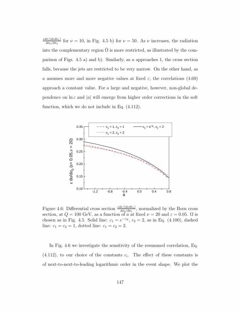
εdσ/(dεdn1)dσ0/dn1
for ν = 10, in Fig. 4.5 b) for ν = 50. As ν increases, the radiation
into the complementary region Ω is more restricted, as illustrated by the com-
parison of Figs. 4.5 a) and b). Similarly, as a approaches 1, the cross section
falls, because the jets are restricted to be very narrow. On the other hand, as
a assumes more and more negative values at fixed ε, the correlations (4.69)
approach a constant value. For a large and negative, however, non-global de-
pendence on ln ε and |a| will emerge from higher order corrections in the soft
function, which we do not include in Eq. (4.112).
-1.2 -0.8 -0.4 0.0 0.4 0.80.10
0.15
0.20
0.25
0.30
0.35 c1 = 1, c2 = 1 c1 = e-γE, c2 = 2
c1 = 2, c2 = 2
ε d σ
/dσ 0
(ε=
0.0
5,ν
= 2
0)
a
Figure 4.6: Differential cross section εdσ/(dεdn1)dσ0/dn1
, normalized by the Born crosssection, at Q = 100 GeV, as a function of a at fixed ν = 20 and ε = 0.05. Ω ischosen as in Fig. 4.5. Solid line: c1 = e−γE , c2 = 2, as in Eq. (4.100), dashedline: c1 = c2 = 1, dotted line: c1 = c2 = 2.
In Fig. 4.6 we investigate the sensitivity of the resummed correlation, Eq.
(4.112), to our choice of the constants ci. The effect of these constants is
of next-to-next-to-leading logarithmic order in the event shape. We plot the
147
differential cross section ε εdσ/(dεdn1)dσ0/dn1
, at Q = 100 GeV, for fixed ε = 0.05 and
ν = 20, as a function of a. The effects of changes in the ci are of the order of
a few percent for moderate values of a.
Finally, we illustrate the sensitivity of these results to the flavor of the
primary partons. For this purpose we study the corresponding ratio of the
shape/flow correlation to the cross section for gluon jets produced by a hy-
pothetical color singlet source. Fig. 4.7 displays the ratio of the differential
cross section dσq(ε, a)/(dεdn1), Eq. (4.112), normalized by the lowest-order
cross section, to the analogous quantity with gluons as primary partons in
the outgoing jets, again at Q = 100 GeV. This ratio is multiplied by CA/CF
in the figure to compensate for the difference in the normalizations of the
lowest-order soft functions. Gluon jets have wider angular extent, and hence
are suppressed relative to quark jets with increasing ν or a, as can be seen by
comparing Figs. 4.7 a) and b). Fig. 4.7 a) shows the ratio at ν = 10, and Fig.
4.7 b) at ν = 50. These results suggest sensitivity to the more complex color
and flavor flow characteristic of hadronic scattering [65, 66].
4.7 Summary and Outlook
We have introduced a general class of inclusive event shapes in e+e− dijet
events which reduce to the thrust and the jet broadening distributions as
special cases. We have derived analytic expressions in transform space, and
have shown the equivalence of our formalism at NLL with the well-known
result for the thrust [57]. Separate studies of this class of event shapes in the
untransformed space, at higher orders, and for nonperturbative effects [60] are
148

a) b)
0.020.04
0.060.08
0.1
e-1.5
-1
-0.5
0
0.5
a1
1.52
2.53
0.020.04
0.060.08e
0.005
0.01
0.015
0.02
e-1.5
-1
-0.5
0
0.5
a
2468
0.005
0.01
0.015e
Figure 4.7: Ratios of differential cross sections for quark to gluon jetsCA
CF
(
εdσq/(dεdn1)dσq
0/dn1
)(
εdσg/(dεdn1)dσg
0/dn1
)−1
at Q = 100 GeV as a function of ε and a
at fixed ν: a) ν = 10, b) ν = 50. Ω as in Fig. 4.5, c1 and c2 as in Eq. (4.100).
certainly of interest. We reserve these studies for future work.
We have introduced a set of correlations of interjet energy flow for the
general class of event shapes, and have shown that for these quantities it is
possible to control the influence of secondary radiation and nonglobal loga-
rithms. These correlations are sensitive mainly to radiation emitted directly
from the primary hard scattering, through transforms in the weight functions
that suppress secondary, or non-global, radiation. We have presented analytic
149

and numerical studies of these shape/flow correlations at leading logarithmic
order in the flow variable and at next-to-leading-logarithmic order in the event
shape. The application of our formalism to multijet events and to scattering
with initial state hadrons is certainly possible, and may shed light on the
relationship between color and energy flow in hard scattering processes with
non-trivial color exchange.
150

Appendix A
A.1 Power counting with contracted vertices
In this appendix we will include the possibility of contracted vertices in the
reduced diagram in Fig. 2.1a. These are associated with internal lines (col-
lapsed to a point) which are off-shell by√
s. Our analysis closely follows [39]
and [43].
If we go back to the argument that led us to Eq. (2.15) for the superficial
degree of IR divergence for the soft part, we see that the same reasoning as in
the case of elementary vertices applies to the case of contracted vertices since
the result (2.15) has been obtained by means of dimensional counting.
The analysis of contracted vertices connecting jet lines only is, however,
more subtle. We have to demonstrate that the suppression factors correspond-
ing to the contracted vertices are at least as great as the ones for the elementary
vertices. The expression (2.22) tells us that we can restrict ourselves to the
two and three point vertices. For these cases, we analyze the full two and
three-point subdiagrams, by studying the tensor structures that are found
after integration over their internal loop momenta.
151
Before we discuss all the possible structures, we state some results which
will be essential for the upcoming analysis. The first one is the simple Dirac
matrix identity
6a 6b 6a = 2(a · b) 6a − a2 6b. (A.1)
The other two follow from Eqs. (2.7) and (2.11) for the gluon propagator
in Coulomb gauge, and hold for any jet momenta scaling as lA ∼ l′A ∼√
s(1+, λ−, λ1/2) collinear to the momentum pA defined in Eq. (2.2)
l′ αA Nαβ(lA, η) = O(λ1/2
√s),
l′ αA Nαβ(lA, η) = O(λ1/2
√s), (A.2)
for all components of β. We now proceed to discuss the particular cases.
Ghost self-energy: The most general covariant structure is, using p · p = p2,
1
Π(p, p) = p · p f(p2/µ2, p2/µ2, αs(µ)), (A.3)
where µ is a scale introduced by a UV/IR regularization of Feynman diagrams
and p is the momentum of an internal jet line. Strictly speaking, the covariants
should be formed from the vectors p and η, but since p has nonzero light-cone
components, we can use Eq. (2.8), to express η in terms of p. The maximum
degree of divergence for the ghost self-energy occurs when the internal lines
become either parallel to the external momentum p or soft. The most general
pinch singular surface consists of a subdiagram of collinear lines moving in
a direction of the external ghost. This subdiagram can interact with itself
1In the rest of this subsection we are concerned the momentum factors only, and we omitdependence on the color structure.
152
through the exchange of soft quanta. Power counting arguments similar to
the ones given in Sec. 2.3.2 show, however, that there is no IR divergence for
these pinch singular points. This shows that the dimensionless function f in
Eq. (A.3) is IR finite. Hence the combination [tree level ghost propagator] -
[ghost self-energy] - [tree level ghost propagator], [1/(p · p)] Π(p, p) [1/(p · p)],
is suppressed at least as much as a single tree level ghost propagator, 1/(p · p).
Therefore the contracted two point ghost vertex within a jet subdiagram con-
tributes at least the same suppression as a single tree level ghost propagator.
Gluon self-energy: With external momentum p, its most general tensor
decomposition has the form
Πµν(p, p) = gµν p2 f1 + pµpν f2 + pµpν f3 + (pµpν + pµpν) f4 . (A.4)
As verified by explicit one-loop calculations in Refs. [49] and [50] the gluon
self-energy in Coulomb gauge is not transverse. In Eq. (A.4), the fi =
fi (p2/µ2, p2/µ2, αs(µ)) are dimensionless functions. Contracting Πµν with
tree level gluon propagators, and using Eq. (2.10), the last two terms in Eq.
(A.4) drop out and the first and the second terms give at least one factor of p2
in the numerator, which cancels one of the (1/p2) denominator factors. Since
the maximum degree of IR divergence for the gluon self-energy occurs when all
the internal lines become either collinear to the external momentum p or soft,
we can use the results of the power counting of Sec. 2.3.2 to demonstrate that
the dimensionless functions fi are at worst logarithmically divergent. There-
fore the combination: gluon jet line - 2 point gluon contracted vertex - gluon
jet line, behaves the same way as a gluon jet line for the purpose of the jet
153

power counting.
Fermion self-energy: In the massless fermion limit, the most general matrix
structure of the fermion self-energy is
Σ(p, p) = 6p g1+ 6 p g2, (A.5)
with dimensionless functions gi = gi(p2/µ2, p2/µ2, αs(µ)), i = 1, 2. When we
sandwich the fermion self-energy between the tree level fermion denominators,
the first term in Eq. (A.5) behaves the same way as the tree level fermion
propagator, modulo logarithmic enhancements due to the function g1. The
second term, however, is absent from the fermion self-energy as was shown
in Ref. [43] using the method of induction and Ward identities. The idea
was to study a variation of the fermion self-energy by making an infinitesimal
Lorentz boost on the external momentum. This implies a relationship between
the (r + 1) and the r-loop self energy. Assuming that the term proportional
to 6p is absent from the r-loop expansion Sen shows that it is also absent from
the (r + 1)-loop expansion. So the first term in Eq. (A.5) is the only possible
structure of the fermion self-energy when its external momentum is jet like
and approaches mass shell.
Now let us investigate the 3 point functions.
Fermion-gluon-fermion vertex function: Γµ, can depend on vectors that scale
as lA, l′A in Eq. (A.2), provided all momenta external to the contracted vertex
are collinear to momentum pA given in Eq. (2.2). It has one Lorentz index, µ,
and neglecting the fermion masses, it contains an odd number of gamma ma-
trices. This implies that the most general tensor and gamma matrix expansion
154

of Γµ involves
1. γµ,
2. γµ 6 lA 6 lA / (lA · lA) and all permutations of γµ, 6 lA, 6 lA,
3. 6 lA lµA / l2A, 6 lA lµA / (lA · lA), 6 lA lµA / (lA · lA), 6 lA lµA / l2A.
The differences between the listed set of structures and other possible combi-
nations are O(λ1/2√
s), as can be shown using Eqs. (A.1)-(A.2). The listed
gamma matrix structures are multiplied by dimensionless functions, which can
depend on the combinations l2A, l2A, l′ 2A , l′ 2
A , besides the renormalization scale
and the running coupling. Using the arguments similar to the ones leading to
Eq. (2.23), we easily verify that the above mentioned dimensionless functions
are at most logarithmically divergent. Next we analyze the possible Dirac
structures.
1. The first case has the same structure as the elementary vertex, and
therefore causes the same suppression as the elementary vertex.
2. The fermion-gluon-fermion composite 3-point vertex is sandwiched be-
tween the factors 6 l′A and 6 lA, originating from the numerators of the
fermion propagators external to the composite vertex. Therefore the
terms from case 2 where 6 lA is on the first or third position in the string
of the gamma matrices provide a suppression√
l2A. On the other hand in
the case, when 6 lA is in the middle of this string of three gamma matrices,
we encounter the combination 6 l′A γµ 6 lA after taking into account the nu-
merators of the external fermions. Using Eq. (A.1), we can immediately
recognize that this combination provides a suppression λ1/2.
155

3. Based on the preceding arguments it is obvious that also the structures
included in item 3 supply at least the same suppression factor as the
elementary vertex.
Therefore, we conclude that the composite 3-point fermion-gluon-fermion ver-
tex behaves as the elementary vertex for the purposes of the jet power counting.
Three gluon vertex: Vµνρ, with external momenta collinear to momen-
tum pA. This vertex can depend on momenta lA, lA defined above and the
metric tensor gαβ. Taking into account the dimension of the 3 gluon Green
function, its only possible tensor structure involves combinations of the form
[gµν lρA + perm. + O(λ1/2√
s)] and [lµA lνA lρA/l2A + O(λ1/2√
s)], with all possible
replacements of lA → lA. These tensor structures are multiplied by dimension-
less functions. The former is the same as in the case of an elementary vertex
and it therefore supplies the same suppression factor as the elementary vertex.
The latter also provides the same suppression as the elementary vertex, since
the two momenta, say lµA, lνA, after being contracted with the propagators of
the external gluons, give suppression factors, as in Eq. (A.2), which cancel the
1/l2A enhancement. The leftover momentum lρA provides the same suppression
factor as the elementary vertex. Using the collinear power counting of Sec.
2.3.2, one can immediately see that the IR divergence of the dimensionless
functions multiplying these tensor structures is not worse than logarithmic.
Hence, there is a suppression factor λ1/2 associated with every contracted 3
gluon vertex.
Ghost - gluon - antighost three point vertex: When all lines external to the
contracted vertex are of the order lA, the most general tensor structure for this
156
contracted vertex is
lµA h1 + lµA h2 + O(λ1/2√
s), (A.6)
with dimensionless functions hi = hi (l2A/µ2, l2A/µ2, αs(µ)), i = 1, 2, which are
at most logarithmically IR divergent. Using Eq. (A.2), we see that when the
momenta in Eq. (A.6) are contracted with the tree level gluon propagator, we
get a suppression of the order of the transverse jet momentum, and that this
contracted vertex gives the same suppression as the elementary three point
vertex, at least.
A.2 Varying the Gauge-Fixing Vector
In this appendix we study the effect of an infinitesimal boost, performed on
the gauge fixing vector η, on an expectation of a time ordered product of fields,
denoted by O, taken between physical states. The gauge-fixing and the ghost
terms in the QCD lagrangian are
Lg.f.(x) = − 1
2ξg2
a(x),
Lghost(x) = −ba(x) δBRS ga(x) /δΛ, (A.7)
respectively. In Eq. (A.7), δΛ is a Grassmann parameter defining the BRS
transformation, ba(x) is an antighost field and
ga(x) ≡ −∂ · Aa(x) ≡ −(∂ − (η · ∂) η) · Aa(x). (A.8)
157
Let us consider an infinitesimal boost with velocity δβ on a gauge fixing vector
η performed in the plus-minus plane
η → η′ ≡ η + η δβ, (A.9)
where the vectors η and η are defined in Eqs. (2.9) and (2.35), respectively.
Since only the gauge fixing and the ghost terms in the QCD lagrangian depend
on η, we can write to accuracy O(δβ2)
δ < O > ≡ < O(η′) > − < O(η) > = < ηα ∂ O
∂ηαδβ >
= − i
ξ
∫
d4x < O(η) ga(x) δga(x) >
− i
∫
d4x < O(η) ba(x) δ (δBRS ga(x)/δΛ) > .
(A.10)
Using the BRS invariance of the QCD lagrangian and the BRS transformation
rule for an antighost field
δBRSba(x)/δΛ =1
ξga(x), (A.11)
we arrive at
δ < O >= −i
∫
d4x < (δBRSO/δΛ) ba(x) δ ga(x) > . (A.12)
158
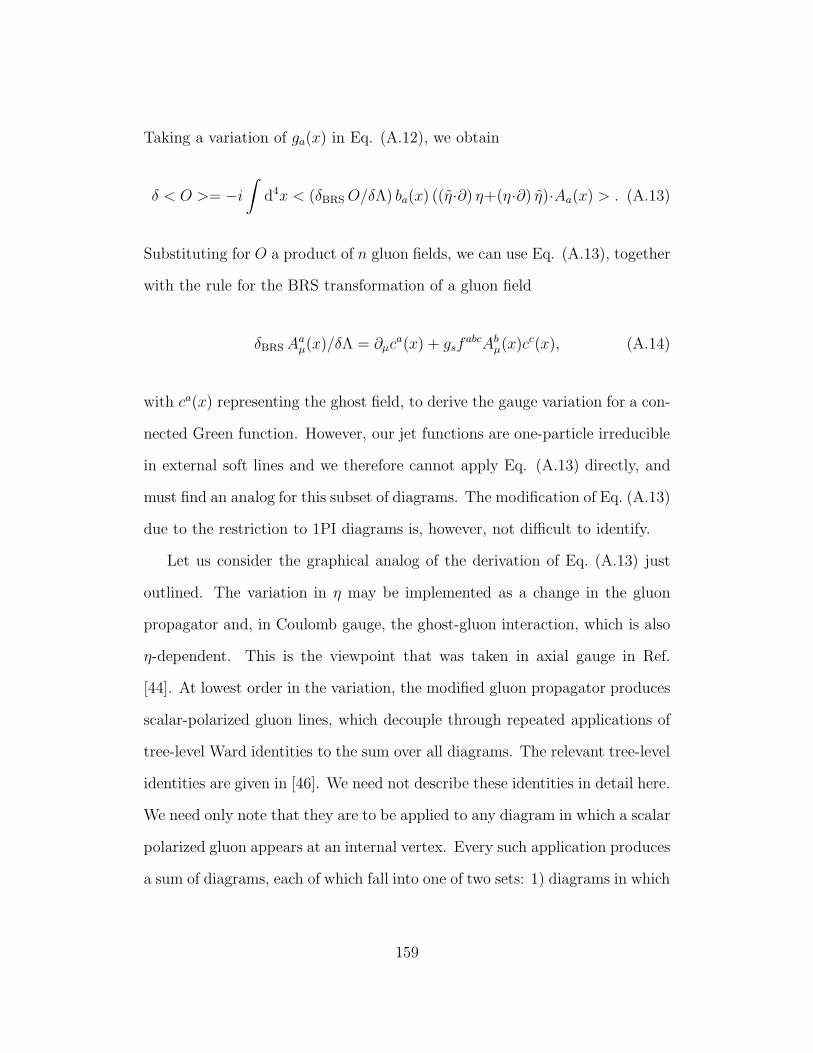
Taking a variation of ga(x) in Eq. (A.12), we obtain
δ < O >= −i
∫
d4x < (δBRS O/δΛ) ba(x) ((η·∂) η+(η·∂) η)·Aa(x) > . (A.13)
Substituting for O a product of n gluon fields, we can use Eq. (A.13), together
with the rule for the BRS transformation of a gluon field
δBRS Aaµ(x)/δΛ = ∂µc
a(x) + gsfabcAb
µ(x)cc(x), (A.14)
with ca(x) representing the ghost field, to derive the gauge variation for a con-
nected Green function. However, our jet functions are one-particle irreducible
in external soft lines and we therefore cannot apply Eq. (A.13) directly, and
must find an analog for this subset of diagrams. The modification of Eq. (A.13)
due to the restriction to 1PI diagrams is, however, not difficult to identify.
Let us consider the graphical analog of the derivation of Eq. (A.13) just
outlined. The variation in η may be implemented as a change in the gluon
propagator and, in Coulomb gauge, the ghost-gluon interaction, which is also
η-dependent. This is the viewpoint that was taken in axial gauge in Ref.
[44]. At lowest order in the variation, the modified gluon propagator produces
scalar-polarized gluon lines, which decouple through repeated applications of
tree-level Ward identities to the sum over all diagrams. The relevant tree-level
identities are given in [46]. We need not describe these identities in detail here.
We need only note that they are to be applied to any diagram in which a scalar
polarized gluon appears at an internal vertex. Every such application produces
a sum of diagrams, each of which fall into one of two sets: 1) diagrams in which
159
an internal gluon line is transformed to a yet another ghost line ending in a
scalar polarization, and 2) diagrams in which one gluon line is contracted to
a point. The new vertex formed in the former case is the ghost term, and in
the latter case it is the ghost-gluon vertex of the BRS variation (A.14). Eq.
(A.13) must result from the cancellation of all diagrams, set 2), in which an
internal gluon line is contracted. Contracted external lines provide the ghost-
gluon terms, and the ghost lines of set 1) eventually provide the ghost terms
of the BRS variations (A.14) of external fields in Eq. (A.13).
The simplicity of the tree level Ward identities puts strong limitations on
the sets of diagrams that can combine to form different diagrammatic contri-
butions to Eq. (A.13). For diagrams of set 1), the topology of the original
diagram is unchanged, and a 1PI diagram remains 1PI. For diagrams of set
2), generally 1PI diagrams remain 1PI, except in the special case of a dia-
gram that is two-particle reducible, with these two lines separated by a single
propagator. In this case, the contraction of the internal line that separates
the other two will bring those two lines together at a single vertex, producing
a diagram precisely of the topology shown in Fig. 2.4. On the one hand, by
Eq. (A.13) all such diagrams must cancel in the full perturbative sum. On
the other hand, the same topology results from a diagram that is one-particle
reducible with respect to a single line, which is then contracted as a result of
the tree-level Ward identity. The latter diagram, however, is not included in
the set of 1PI diagrams with which we work. The application of the Ward
identity to 1PI diagrams only, therefore, results in terms that would cancel
this special set of one-particle reducible diagrams, in which the only line that
spoils irreducibility is contracted to a point. These are the diagrams shown
160

T3BA T1
BA
T2BA
a) b) )Figure A.1: Two-loop diagram illustrating the idea of the tulip-garden for-malism. T1, T2, T3 are the possible tulips.
in Fig. 2.4, in which the ghost-gluon vertex of Eq. (A.14) is inserted between
one-particle irreducible subdiagrams in all possible ways. The ghost line end-
ing at this composite vertex is continuously connected to the variation of a
gluon propagator, according to Eq. (A.13). The full composite vertex of the
Ward identity in Eq. (A.13) appears only at true external lines of the 1PI jet.
This vertex is given by the momentum factor in Eq. (2.37) and is represented
by the double line crossing a gluon line in Fig. A.2 below. Diagrams that are
reducible in one or more internal lines can be treated in a similar manner. The
“left-over” terms in the Ward identities for each set of diagrams of definite re-
ducibility properties (1PI, 2PI, etc.), must cancel in the full sum, reproducing
the identity for Green functions, Eq. (A.13).
A.3 Tulip-Garden Formalism
In this appendix we illustrate how a given Feynman diagram contributing to
the process (2.1) in the leading power can be systematically written in the
form (2.27). For concreteness let us consider a two loop diagram where the
quarks interact via the exchange of a one rung gluon ladder as in Fig. A.1.
161

The important contributions of this diagram come from the regions when all
of the exchanged gluons are soft, Fig. A.1a or when the gluons attached to the
A quark line are soft, while the rest of the gluons carries momenta parallel to
the − direction (they belong to jet B), Fig. A.1b, or when the two gluon lines
attached to the B quark line are soft and the other gluons are collinear to the +
direction (they belong to jet A), Fig. A.1c. The possible central soft exchange
parts are called tulips. In our case the possible tulips are denoted as T1, T2, T3
in Fig. A.1. The garden is defined as a nested set of tulips T1, . . . , Tn such
that Ti ⊂ Ti+1 for i = 1, . . . , n − 1. In Fig. A.1, T1, T2, T3, T1, T3,
T2, T3 are the possible gardens.
For a given tulip we make the soft approximation, consisting of attaching a
soft gluon to jet A via the − component of its polarization only and to jet B via
the the + component of its polarization. The result of this soft approximation
for a given Feynman diagram F corresponding to a tulip T is denoted S(T )F .
It has obviously the form of Eq. (2.27). Following the prescription given in
Refs. [44] and [16] we write the contribution to a given diagram F in the form
F =∑
G
(−1)n+1S(T1) . . . S(Tn) F + FR, (A.15)
where the sum over inequivalent gardens, as defined bellow, G in Eq. (A.15)
is understood. The meaning of this expression is the following. For a given
garden consisting of a set of tulips T1, . . . , Tn, we start with the largest tulip
Tn and make the soft approximation for the gluon lines coming out of it. Then
for Tn−1 we proceed the same way as for Tn. If some of the lines coming out
of Tn−1 are identical to the ones coming out of Tn we leave them untouched.
162

For instance, if we consider a garden T2, T3 from Fig. A.1, we first perform
the soft approximation on tulip T3 and then proceed to tulip T2. However the
lines coming out of T2 and T3 which attach to the B quark line are identical so
when performing S(T2)S(T3)F we leave these gluon lines out of the game and
make soft approximations only on the gluon lines attaching to the ladder’s
rung. Two gardens are equivalent if the soft approximation is identical for
both of them. FR is defined by Eq. (A.15). The contribution to FR comes
from the integration region where |~k| &√
s for all gluons coming out of the
central soft part. As a result, the contribution to FR is suppressed by positive
powers of√−t/
√s. Therefore we can ignore the contribution from FR within
the accuracy at which we are working.
We can now rewrite Eq. (A.15), as
F =∑
T
(
∑
G,Tn=T
(−1)n+1 S(T1) . . . S(Tn−1)
)
S(T ) F + FR. (A.16)
This expression is indeed in the form of Eq. (2.27) since the term S(T )F is of
that form and the subtractions∑
(−1)n+1S(T1) . . . S(Tn−1) modify only the
soft function S in Eq. (2.27), but do not alter the form of the equation. We
can therefore conclude that the contribution to a given Feynman diagram in
leading power can be expressed in the first factorized form given by Eq. (2.27).
A.4 Feynman Rules
In Fig. A.2, we list the Feynman rules for the lines and the vertices encoun-
tered in the text. The double lines are eikonal lines, while the dashed lines
163
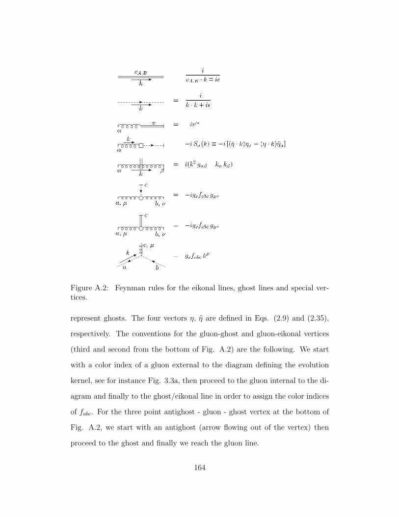
vA;Bk = ivA;B k ik = ik k + i v = iv k = i S(k) i [(~ k) + ( k)~ k = i(k2 g k k)a; b; = igsfab ga; b; = igsfab gka b ; = gsfab kFigure A.2: Feynman rules for the eikonal lines, ghost lines and special ver-tices.
represent ghosts. The four vectors η, η are defined in Eqs. (2.9) and (2.35),
respectively. The conventions for the gluon-ghost and gluon-eikonal vertices
(third and second from the bottom of Fig. A.2) are the following. We start
with a color index of a gluon external to the diagram defining the evolution
kernel, see for instance Fig. 3.3a, then proceed to the gluon internal to the di-
agram and finally to the ghost/eikonal line in order to assign the color indices
of fabc. For the three point antighost - gluon - ghost vertex at the bottom of
Fig. A.2, we start with an antighost (arrow flowing out of the vertex) then
proceed to the ghost and finally we reach the gluon line.
164
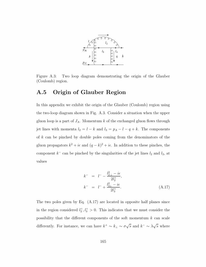
pApB k q kl1l l2 l3Figure A.3: Two loop diagram demonstrating the origin of the Glauber(Coulomb) region.
A.5 Origin of Glauber Region
In this appendix we exhibit the origin of the Glauber (Coulomb) region using
the two-loop diagram shown in Fig. A.3. Consider a situation when the upper
gluon loop is a part of JA. Momentum k of the exchanged gluon flows through
jet lines with momenta l2 = l − k and l3 = pA − l − q + k. The components
of k can be pinched by double poles coming from the denominators of the
gluon propagators k2 + iǫ and (q − k)2 + iǫ. In addition to these pinches, the
component k− can be pinched by the singularities of the jet lines l2 and l3, at
values
k− = l− − l22⊥ − iǫ
2l+2,
k− = l− +l23⊥ − iǫ
2l+3. (A.17)
The two poles given by Eq. (A.17) are located in opposite half planes since
in the region considered l+2 , l+3 > 0. This indicates that we must consider the
possibility that the different components of the soft momentum k can scale
differently. For instance, we can have k+ ∼ k⊥ ∼ σ√
s and k− ∼ λ√
s where
165

λ ≪ σ ≪ 1. Indeed, the power counting performed in Sec. 2.3.2 shows
that the singularities originating from these regions can produce a logarithmic
enhancement. We also note that it is only minus components that are pinched
in this way by the lines in JA, and plus components by the lines in JB.
166
Appendix B
B.1 Symmetry property of the jet functions
Here we prove Eq. (3.45). In order to do so, we first shift the momentum
of J(n)A in the transverse direction: pA → pA + q. This does not effect the
logarithmic behavior of the jet function, but it makes easier the comparison
of diagrams from J(n)A and J
(n)A .
The general diagram contributing to the jet function J(n)A has the form
shown in Fig. B.1. There are N gluons connecting the quark line to the rest
of the diagram, which contains L loops. For every diagram contributing to
J(n)A , we identify the corresponding diagram from J
(n)A . The guide is that they
should be a mirror image of each other, but they should have the same color
structure. For instance, in the case of a one loop contribution to J(2)A shown
in Fig. B.2a the related diagram from J(2)A is the one in Fig. B.2b.
Let us now make a transformation in J(n)A (pA + q, η):
k±i → −k±
i , ki⊥ → ki⊥ for all i = 1, . . . , n . (B.1)
167

pA pA qp1 pN11 Nk1 kn
Figure B.1: General class of diagrams contributing to J(n)A .
In the denominators of the propagators this transformation can be compen-
sated by a similar transformation of loop momenta l±j → −l±j and lj ⊥ → lj ⊥
for j = 1, . . . , (L + N − 1). The three-point vertices in the L-loop subdiagram
generate a factor (−1)v3 under this set of transformations. Using the relation-
ship between the number of loops, vertices and external lines on the L-loop
subdiagram:
v3 = N + n + 2(L − v4 − 1), (B.2)
we see that
(−1)v3 = (−1)N+n. (B.3)
We also have to identify the relationship between the strings of gamma ma-
trices on the fermion line
J(n,0)A ≡ u(pA − q, λ1) γµN
(
1∏
i=N−1
6pi γµi
)
u(pA, λA), (B.4)
168

pA pA qkl l kpA l q k pA + q pAq k
l k lpA l ka) b)Figure B.2: Identification of a particular one loop diagram between the jetfunctions J
(2)A and J
(2)A .
in J(n)A , and
J(n,0)A ≡ v(pA + q, λA) γµN
(
1∏
i=N−1
(− 6pi) γµi
)
v(pA, λ1), (B.5)
in J(n)A . Using the charge conjugation matrix C and its properties, Ref. [51]:
γTµ = − CγµC
−1,
CT = − C,
vα(p, λ) = (−1)λ+1/2 Cαβuβ(p, λ),
uα(p, λ) = (−1)λ+1/2 Cαβvβ(p, λ), (B.6)
we obtain
J(n,0)A = (−1)N (−1)2N−1(−1)λA+λ1 u(pA, λ1)
(
N−1∏
i=1
γµi6pi
)
γµNu(pA+q, λA).
(B.7)
In the Regge limit, we can neglect the momentum q in the numerators. Since
all the momenta pi are collinear to pA, J(n,0)A is symmetric under the exchange of
169

its external Lorentz indices. Therefore, up to the power-suppressed corrections,
we have:
J(n,0)A = (−1)N−1 (−1)λA+λ1 J
(n,0)A (B.8)
Combining Eqs. (B.3) and (B.8), we immediately recover Eq. (3.45).
B.2 Evolution kernel
In this appendix we provide the calculational details of the results given in
Sec. 3.3.2.
The contribution to Fig. 3.9b is:
Fig. 3.9b ≡ ig3s t facb ffbd fcfe
∫
dDk
(2π)D
dDl
(2π)DJ
(2) d eA (pA, q; l+ = 0, l−, l⊥)
×(
N− µ(l)
l2(l − k)µ
N− ν(q − l)
(q − l)2(q − k)ν
k+
(l − k)2
)
(k+ = 0)
× N− ρ(k)
k2
Sρ(k)
k · k1
k− − iǫ
1
(q − k)2= 0. (B.9)
Note that the overall sign in Eq. (B.9) reflects the minus sign explicit in Fig.
3.9b.
We analyze the diagram in Fig. 3.9c in a similar way. It takes the form:
Fig. 3.9c ≡ −ig3s t facb ffbd fcfe
∫
dDk
(2π)D
dDl
(2π)DJ
(2) d eA (pA, q; l+ = 0, l−, l⊥)
×(
N−µ(l)
l2(l − k)µ
N−+(q − l)
(q − l)2
1
(l − k)2
)
(k+ = 0)
× N− ρ(k)
k2
Sρ(k)
k · k1
k− − iǫ. (B.10)
170

Note, again, that the overall sign in Eq. (B.10) reflects the minus sign explicit
in Fig. 3.9c. The imaginary part of the eikonal propagator in Eq. (B.10) gives
vanishing contribution since the resulting integrand is an odd function under
k+ → −k+. Hence only the principal value part contributes. In the Glauber
region, l− ≪ l+ ∼ l⊥, the integral vanishes due to the antisymmetry of the
integrand under the transformation l+ → −l+, k± → −k±. In the region
l− ∼ l+ ∼ l⊥ we can factor the gluon with momentum l from the jet J(2)A .
The contribution to Fig. 3.10a from a G gluon with momentum k corre-
sponding to the first term in Eq. (3.50) and to Fig. 3.8a is:
(Fig. 3.10a)G ≡ g2s t fade febc
∫
dDk
(2π)D
dDl
(2π)DSG(k, l, q)
× J(3) b c dA (pA, q; k+ = 0, k−, k⊥, l+ = 0, l−, l⊥), (B.11)
with the soft function SG in Eq. (B.11) defined as
SG(k, l, q) ≡(
N− µ(l)
l2Vµρν(l,−k, k − l)
Nν −(k − l)
(k − l)2
(
gρ + − kρ
k−
))
(k+ = 0)
× N−α(k)
k2
Sα(k)
k · kN−+(q − k)
(q − k)2. (B.12)
Since, by construction k− ∼ k+ ∼ k⊥ for an external G gluon with momentum
k, we can factor the gluon with momentum q−k from J(3)A in Fig. 3.10a. Then
the resulting integrand in Eq. (B.11); SG(k, l, q)/k−, with SG defined in Eq.
(B.12); is an antisymmetric function under the transformation k± → −k±,
l+ → −l+ in the Glauber region l− ≪ l+ ∼ l⊥. This indicates that the gluon
with momentum l can be factored from J(3)A . Therefore the contribution to
Fig. 3.10a from a G gluon agrees with a gluon reggeization at NLL.
171
The contribution to Fig. 3.10c is:
(Fig. 3.10c)G ≡ ig3s t facb ffbd fcfe ×
∫
dDk
(2π)D
dDl
(2π)DJ
(2) d eA (pA, q; l+ = 0, l−, l⊥)
×[
N− µ(l)
l2Vµρσ(l,−k, k − l)
(
gρ+ − kρ
k−
)
Nσ λ(l − k)
(l − k)2
× Vνλ−(q − l, l − k, k − q)Nν −(q − l)
(q − l)2
]
(k+ = 0)
× N−α(k)
k2
Sα(k)
k · kN−+(q − k)
(q − k)2. (B.13)
In the Glauber region the l+ integral vanishes due to the antisymmetry of the
integrand. In the region l− ∼ l+ ∼ l⊥ the gluon with momentum l factors out
and the contribution takes a factorized form.
The diagram in Fig. 3.10d for a G gluon with momentum k is:
(Fig. 3.10d)G ≡ −ig3s t faed ×
∫
dDk
(2π)D
dDl
(2π)DJ
(2) b cA (pA, q; l+ = 0, l−, l⊥)
× N−µ(q − l)
(q − l)2W bedc
µρ−ν
(
gρ+ − kρ
k−
)
(k+ = 0)Nν −(l)
l2
× N−α(k)
k2
Sα(k)
k · kN−+(q − k)
(q − k)2,
(B.14)
where
W bedcµρ−ν ≡ fpbe fpdc (gµ−gρν − gµνgρ−) + fpbd fpce (gµνgρ− − gµρgν−)
+ fpbc fped (gµρgν− − gµ−gρν) , (B.15)
is the Lorentz and the color part of the four point gluon vertex. In the Glauber
region the integral over l+ vanishes due to the antisymmetry of the integrand
172
in Eq. (B.14). In the region l− ∼ l+ ∼ l⊥ we can factor the gluon with
momentum l from the jet function J(2)A . Therefore the contribution from Fig.
3.10d is in accordance with gluon reggeization.
The contribution to Fig. 3.10a from the second term in Eq. (3.50) used in
Eq. (3.49) is:
(Fig. 3.10a)soft ≡ g2s t fade febc
∫
dDk
(2π)D
dDl
(2π)DS(a)
s (k, l, q)
× J(3) b c dA (pA, q; k+ = 0, k−, k⊥, l+ = 0, l−, l⊥), (B.16)
with the soft function S(a)s defined by
S(a)s (k, l, q) ≡
[(
N−µ(l)
l2Vµρν(l,−k, k − l)
Nν −(k − l)
(k − l)2
)
(k+)−(
N−µ(l)
l2Vµρν(l,−k, k − l)
Nν −(k − l)
(k − l)2
)
(k+ = 0)
]
× N−α(k)
k2
Sα(k)
k · kN−+(q − k)
(q − k)2. (B.17)
Eqs. (B.16) and (B.17) immediately follow form Eqs. (B.11) and (B.12). We
apply the following identity
S(l−, k−) = S(l− = 0, k− = 0) θ(M − |l−|) θ(M − |k−|)
+ [S(l−, k− = 0) − S(l− = 0, k− = 0) θ(M − |l−|)] θ(M − |k−|)
+ [S(l− = 0, k−) − S(l− = 0, k− = 0) θ(M − |k−|)] θ(M − |l−|)
+ [S(l−, k−) − S(l−, k− = 0) θ(M − |k−|)−
S(l− = 0, k−) − S(l− = 0, k− = 0) θ(M − |k−|) θ(M − |l−|)],
(B.18)
173

to the soft function S(a)s , Eq. (B.17), to analyze the contribution to Eq. (B.16).
After using the first term of Eq. (B.18) for the soft function S(a)s in Eq. (B.16),
we arrive at
(Fig. 3.10a)(1)soft ≡ g2
s t fade febc
∫
dD−2k⊥(2π)D
dD−2l⊥(2π)D
×(∫
dk+ dl+ S(a)s (k+, l+, k− = 0, l− = 0, k⊥, l⊥, q)
)
× Γ(3) b c dA (pA, q; k⊥, l⊥). (B.19)
Performing the k+ and l+ integrals, we obtain
(Fig. 3.10a)(1)soft ≡ −αs
8πt fade febc
∫
dD−2k⊥(2π)D−2
dD−2l⊥(2π)D−2
(|k⊥| − |q⊥ − k⊥ − l⊥|)|k⊥|2 |q⊥ − k⊥ − l⊥|2
× (|k⊥| − |q⊥ − l⊥| + |q⊥ − k⊥ − l⊥|) (|k⊥| + |l⊥| + 2|q⊥ − l⊥| + |q⊥ − k⊥ − l⊥|)|q⊥ − l⊥| (|l⊥| + |q⊥ − l⊥|)2 (|k⊥| + |l⊥| + |q⊥ − k⊥ − l⊥|)
× 1
(|k⊥| + |q⊥ − l⊥| + |q⊥ − k⊥ − l⊥|)Γ
(3) b c dA (pA, q; k⊥, l⊥). (B.20)
When analyzing the second (third) term in Eq. (B.18), after used in Eq.
(B.16), we can factor the gluon with momentum l (k) from the jet function
J(3)A . The resulting l±, k+ (k±, l+) integral is over an antisymmetric function
under the transformation l± → −l±, k+ → −k+ (k± → −k±, l+ → −l+)
and therefore it vanishes. In the case of the last term in Eq. (B.18), we can
factor both gluons with momenta k and l from the jet J(3)A . So this part is in
agreement with gluon reggeization.
The contribution to Fig. 3.10b from the second term in Eq. (3.50) used in
174
Eq. (3.49) is:
(Fig. 3.10b)soft ≡ −g2s t faeb fced
∫
dDk
(2π)D
dDl
(2π)DS(b)
s (k, l, q)
× J(3) b c dA (pA, q; k+ = 0, k−, k⊥, l+ = 0, l−, l⊥),
(B.21)
with the soft function S(b)s (k, l, q) defined by
S(b)s (k, l, q) ≡
[(
N−µ(k − l)
(k − l)2Vµ−ν(k − l, l − q, q − k)
Nν −(q − k)
(q − k)2
)
(k+)−(
N−µ(k − l)
(k − l)2Vµ−ν(k − l, l − q, q − k)
Nν −(q − k)
(q − k)2
)
(k+ = 0)
]
× N−α(l)
l2Sα(l)
l · lN−+(q − l)
(q − l)2. (B.22)
We apply the identity (B.18) to the soft function S(b)s , Eq. (B.22), to analyze
the contribution to Eq. (B.21). After using the first term of Eq. (B.18) in Eq.
(B.21), we arrive at a contribution
(Fig. 3.10b)(1)soft ≡ −g2
s t faeb fced
∫
dD−2k⊥(2π)D
dD−2l⊥(2π)D
×(∫
dk+ dl+ S(b)s (k+, l+, k− = 0, l− = 0, k⊥, l⊥, q)
)
× Γ(3) b c dA (pA, q; k⊥, l⊥). (B.23)
175

Performing the k+ and l+ integrals, we obtain
(Fig. 3.10b)(1)soft ≡ αs
8πt fabe fedc
∫
dD−2k⊥(2π)D
dD−2l⊥(2π)D
× (2|k⊥| + |l⊥| + |q⊥ − k⊥| + |q⊥ − k⊥ − l⊥|)|k⊥| |l⊥|2 |q⊥ − k⊥ − l⊥|2 (|l⊥| + |q⊥ − k⊥| + |q⊥ − k⊥ − l⊥|)
× (|l⊥|3 − |l⊥| (|q⊥ − k⊥|2 + |q⊥ − k⊥ − l⊥|2) − 2|q⊥ − k⊥|2|q⊥ − k⊥ − l⊥|)(|k⊥| + |l⊥| + |q⊥ − k⊥ − l⊥|)2 (|k⊥| + |q⊥ − k⊥|)2
× Γ(3) b c dA (pA, q; k⊥, l⊥). (B.24)
When analyzing the second (third) term in Eq. (B.18), when applied to Eq.
(B.21), we can factor the gluon with momentum l (k) from the jet function
J(3)A . The resulting l±, k+ (k±, l+) integral is over a function antisymmetric
under the transformation l± → −l±, k+ → −k+ (k± → −k±, l+ → −l+)
and therefore it vanishes. In the case of the last term in Eq. (B.18), we can
factor both gluons with momenta k and l from the jet J(3)A . So this part is in
agreement with the gluon reggeization.
The contribution to Fig. 3.10c from the second term in Eq. (3.50) used in
Eq. (3.49) is:
(Fig. 3.10c)soft ≡ ig3s t facb ffbd fcfe ×
∫
dDk
(2π)D
dDl
(2π)DJ
(2) d eA (pA, q; l+ = 0, l−, l⊥)
×[(
N−µ(l)
l2Vµ−σ(l,−k, k − l)
Nσ λ(l − k)
(l − k)2Vνλ−(q − l, l − k, k − q)
Nν −(q − l)
(q − l)2
)
(k+)
−(
N−µ(l)
l2Vµ−σ(l,−k, k − l)
Nσ λ(l − k)
(l − k)2Vνλ−(q − l, l − k, k − q)
Nν −(q − l)
(q − l)2
)
(k+ = 0)
]
× N−α(k)
k2
Sα(k)
k · kN−+(q − k)
(q − k)2.
(B.25)
176

This follows immediately from Eq. (B.13). In the Glauber region, l− ≪ l+ ∼
l⊥, the integrand is an antisymmetric function of k± and l+ and therefore the
k±, l+ integral vanishes. In the region l− ∼ l+ ∼ l⊥, we can factor the gluon
with momentum l from the jet function J(2)A . Hence this contribution is in
agreement with gluon reggeization.
The contribution to Fig. 3.10a from the third term in Eq. (3.50) used in
Eq. (3.49) is:
(Fig. 3.10a)soft′ ≡ g2s t fade febc
∫
dDk
(2π)D
dDl
(2π)DS
(a)s′
× J(3) b c dA (pA, q; k+ = 0, k−, k⊥, l+ = 0, l−, l⊥),
(B.26)
with the soft function S(a)s′ defined by
S(a)s′ ≡ N− µ(l)
l2(Vµρν(l,−k, k − l) − g+ρ Vµ−ν(l,−k, k − l))
Nν −(k − l)
(k − l)2
× Nρ α(k)
k2
Sα(k)
k · kN−+(q − k)
(q − k)2. (B.27)
This follows immediately from Eqs. (B.11) and (B.12). We apply the identity
(B.18) to the soft function S(a)s′ , Eq. (B.27), to analyze the contribution to Eq.
(B.26). After using the first term of Eq. (B.18) in Eq. (B.26), we arrive at
(Fig. 3.10a)(1)soft′ ≡ g2
s t fade febc
∫
dD−2k⊥(2π)D
dD−2l⊥(2π)D
×(∫
dk+ dl+ S(a)s′ (k+, l+, k− = 0, l− = 0, k⊥, l⊥, q)
)
× Γ(3) b c dA (pA, q; k⊥, l⊥). (B.28)
177

The integrand S(a)s′ in Eq. (B.28) is an antisymmetric function of l+ and k+
and therefore the integral over k+ and l+ in Eq. (B.28) vanishes. In order to
show this antisymmetry, we have used that the component
N+ α(k− = 0, k+, k⊥) Sα(k− = 0, k+, k⊥) = 0, (B.29)
in the Glauber region, k− ∼ 0. We have also used the Ward identity
lµkρVµρν(l,−k, k − l)(k − l)ν = 0, (B.30)
when analyzing the contribution from the transverse polarization of the gluon
with momentum k in Fig. 3.10a. When studying the second (third) term in Eq.
(B.18), after applied to Eq. (B.26), we can factor the gluon with momentum
l (k) from the jet function J(3)A . The resulting l±, k+ (k±, l+) integral is over
an antisymmetric function under the transformation l± → −l±, k+ → −k+
(k± → −k±, l+ → −l+) and therefore it vanishes. In the case of the last term
in Eq. (B.18), we can factor both gluons with momenta k and l from the jet
J(3)A . Therefore the contribution from (Fig. 3.10a)soft′, Eq. (B.26), is in an
agreement with gluon reggeization at NLL.
The contribution to Fig. 3.10b from the third term in Eq. (3.50) used in
Eq. (3.49) is:
(Fig. 3.10b)soft′ ≡ −g2s t faeb fced
∫
dDk
(2π)D
dDl
(2π)DS
(b)s′
× J(3) b c dA (pA, q; k+ = 0, k−, k⊥, l+ = 0, l−, l⊥), (B.31)
178

with the soft function S(b)s′ defined by
S(b)s′ ≡ N−µ(k − l)
(k − l)2(Vµρν(k − l, l − q, q − k) − g+ρ Vµ−ν(k − l, l − q, q − k))
× Nν −(q − k)
(q − k)2
N−α(l)
l2Sα(l)
l · lNρ +(q − l)
(q − l)2. (B.32)
This follows from Eqs. (B.21) and (B.22). We apply the identity (B.18) to the
soft function, Eq. (B.32), to analyze the contribution to Eq. (B.31). After
using the first term of Eq. (B.18) in Eq. (B.31), we arrive at
(Fig. 3.10b)(1)soft′ ≡ −g2
s t faeb fced
∫
dD−2k⊥(2π)D
dD−2l⊥(2π)D
×(∫
dk+ dl+ S(b)s′ (k+, l+, k− = 0, l− = 0, k⊥, l⊥, q)
)
× Γ(3) b c dA (pA, q; k⊥, l⊥). (B.33)
The integrand S(b)s′ in Eq. (B.33) is an antisymmetric function of l+ and k+
and therefore the integral over k+ and l+ in Eq. (B.33) vanishes. In order to
show this antisymmetry, we have used that the component N++(q − l) = 0 in
the Glauber region, l− ∼ 0. We have also used the Ward identity
(k − l)µ(l − q)ρVµρν(k − l, l − q, q − k)(q − k)ν = 0, (B.34)
when analyzing the contribution from the transverse polarization of the gluon
with momentum q − l in Fig. 3.10b. When analyzing the second (third) term
in Eq. (B.18), applied to Eq. (B.31), we can factor the gluon with momentum
l (k) out the jet function J(3)A . The resulting l±, k+ (k±, l+) integral is over
an antisymmetric function under the transformation l± → −l±, k+ → −k+
179

(k± → −k±, l+ → −l+) and therefore it vanishes. In the case of the last term
in Eq. (B.18), we can factor both gluons with momenta k and l from the jet
J(3)A . Therefore the contribution from (Fig. 3.10b)soft′ , Eq. (B.31), is in an
agreement with gluon reggeization at NLL.
The contribution to Fig. 3.10c from the third term in Eq. (3.50) used in
Eq. (3.49) is:
(Fig. 3.10c)soft′ ≡ ig3s t facb ffbd fcfe ×
∫
dDk
(2π)D
dDl
(2π)D
× J(2) d eA (pA, q; l+ = 0, l−, l⊥)
N−µ(l)
l2
× (Vµβσ(l,−k, k − l) − g−β Vµ−σ(l,−k, k − l))Nσ λ(l − k)
(l − k)2
× (Vνλγ(q − l, l − k, k − q) − g−γ Vνλ−(q − l, l − k, k − q))
× Nν −(q − l)
(q − l)2
Nβ α(k)
k2
Sα(k)
k · kNγ +(q − k)
(q − k)2. (B.35)
In the Glauber region, l− ≪ l+ ∼ l⊥, the integrand is an antisymmetric
function of k± and l+ and therefore the k±, l+ integral vanishes. In the region
l− ∼ l+ ∼ l⊥, we can factor the gluon with momentum l out the jet function
J(2)A . Hence this contribution is in agreement with gluon reggeization.
The diagram in Fig. 3.10d from the third term in Eq. (3.50) used in Eq.
(3.49) is:
(Fig. 3.10d)soft′ ≡ −ig3s t faed ×
∫
dDk
(2π)D
dDl
(2π)DJ
(2) b cA (pA, q; l+ = 0, l−, l⊥)
× N−µ(q − l)
(q − l)2
(
W bedcµρσν − g−ρ g−σ W bedc
µ−−ν
) Nν −(l)
l2Nρ α(k)
k2
× Sα(k)
k · kNσ +(q − k)
(q − k)2, (B.36)
180

In the Glauber region, l− ≪ l+ ∼ l⊥, the integrand is an antisymmetric
function of k± and l+ and therefore the k±, l+ integral vanishes. In the region
l− ∼ l+ ∼ l⊥, we can factor the gluon with momentum l out the jet function
J(2)A . Hence this contribution is in agreement with gluon reggeization.
The contribution from the first term in Eq. (3.51) is:
(Fig. 3.8c)jet ≡ g2s t fade febc
∫
dDk
(2π)D
dDl
(2π)DSjet(k, l, q)
× J(3) b c dA (pA, q; k+ = 0, k−, k⊥, l+ = 0, l−, l⊥),
(B.37)
with a soft function Sjet defined
Sjet(k, l, q) ≡ N−µ(k)
k2
Sµ(k)
k · kN−α(q − l − k)
(q − l − k)2
(q − l)α
(l − q) · (l − q)
N−+(l)
l2.
(B.38)
Next we use an identity (B.18) for Sjet(k−, l−), defined in Eq. (B.38). After
performing the k+ and l+ integrals in the first term of Eq. (B.18), when used
181
in Eq. (B.37), we obtain the following contribution:
(Fig. 3.8c)(1)jet ≡ −αs
8πt fade febc
∫
dD−2k⊥(2π)D−2
dD−2l⊥(2π)D−2
Γ(3) b c dA (pA, q; k⊥, l⊥)
×[
(|k⊥| + |l⊥| + |q⊥ − l⊥| + 2|q⊥ − k⊥ − l⊥|)|k⊥| |q⊥ − k⊥ − l⊥| (|l⊥| + |q⊥ − l⊥|) (|k⊥| + |q⊥ − k⊥| + |q⊥ − k⊥ − l⊥|)2
× (|k⊥|2 − |q⊥ − l⊥|2 + |q⊥ − k⊥ − l⊥|2)(|k⊥| + |q⊥ − l⊥| + |q⊥ − k⊥ − l⊥|)2 |q⊥ − k⊥ − l⊥|2
+
( |l⊥| + 2|q⊥ − k⊥ − l⊥|(|l⊥| + |q⊥ − k⊥ − l⊥|) (|k⊥| + |l⊥| + |q⊥ − k⊥ − l⊥|)2
− |q⊥ − l⊥| + 2|q⊥ − k⊥ − l⊥|(|q⊥ − l⊥| + |q⊥ − k⊥ − l⊥|) (|k⊥| + |q⊥ − l⊥| + |q⊥ − k⊥ − l⊥|)2
)
× (|k⊥|2 − |q⊥ − l⊥|2 − |q⊥ − k⊥ − l⊥|2)|k⊥| (|l⊥|2 − |q⊥ − l⊥|2) |q⊥ − k⊥ − l⊥|3
]
. (B.39)
In the second (third) term of Eq. (B.18), we can factor the gluon with momen-
tum l (k) from the jet function J(3)A . The resulting l±, k+ (k±, l+) integrals
are over antisymmetric functions and therefore they vanish. In the last term
of Eq. (B.18), we can factor both gluons with momenta k and l from the jet
function J(3)A . Hence this contribution is in a factorized form, in agreement
with the gluon reggeization.
The contribution to the second term in Eq. (3.51) comes from a diagram
in Fig. 3.10e:
Fig. 3.10e = ig3s t faeb fbcf ffdc ×
∫
dDk
(2π)D
dDl
(2π)DJ
(2) d eA (pA, q; l+ = 0, l−, l⊥)
× N−µ(q − l)
(q − l)2Vµνρ(q − l,−k, k + l − q)
Nν α(k)
k2
Sα(k)
k · k
× Nρ σ(q − l − k)
(q − l − k)2
(l − q)σ
(l − q) · (l − q)
N−+(l)
l2. (B.40)
In the Glauber region l− ≪ l+ ∼ l⊥, the integrand is an antisymmetric function
182

under the transformation k± → −k± and l+ → −l+, so the integral over
k± and l+ vanishes. In the region l− ∼ l+ ∼ l⊥ we can factor the gluon
with momentum l from the jet function J(2)A using the K-G decomposition.
Therefore the contribution from Fig. 3.10e takes a factorized form.
The same reasoning applies to the diagram in Fig. 3.10f, which is due to
the third term in Eq. (3.51):
Fig. 3.10f = ig3s t fabc fcdf ffbe ×
∫
dDk
(2π)D
dDl
(2π)DJ
(2) d eA (pA, q; k+ = 0, k−, k⊥)
× N−α(k)
k2
Sα(k)
k · kN−µ(q − k)
(q − k)2Vµνρ(q − k, k + l − q,−l)
Nρ +(l)
l2
× Nν σ(q − l − k)
(q − l − k)2
(l − q)σ
(l − q) · (l − q). (B.41)
It also factorizes in agreement with the gluon reggeization hypothesis.
183
Appendix C
C.1 Eikonal Example
In this appendix, we give details of the calculation of the logarithmic behavior
in the diagrams of Fig. 4.3. We choose the reference frame such that the
momenta of the final state particles are given by:
β1 = (1, 0, 0, 1),
β2 = (1, 0, 0,−1),
l = ωl(1, sl, 0, cl),
k = ωk(1, sk cos φ, sk sin φ, ck). (C.1)
Here we define sl,k ≡ sin θl,k and cl,k ≡ cos θl,k. θl is the angle between the
vectors ~l and ~β1, θk is the angle between the vectors ~k and ~β1 and φ is the
azimuthal angle of the gluon with momentum k relative to the plane defined
by β1, β2 and l. The available phase space in polar angle for the radiated
gluons is θk ∈ (π/2 − δ, π/2 + δ) and θl ∈ (0, π/2 − δ) ∪ (π/2 + δ, π).
Using the diagrammatic rules for eikonal lines and vertices, as listed for ex-
184

ample in [8], we can write down the expressions corresponding to each diagram
separately. For example, diagram 4.3 a) gives
a) + (k ↔ l) = [fabcTr(tatbtc)](
−ig4s βα
1 ββ2 βγ
1
)
Vαβγ(k + l,−k,−l)
× 1
β1 · (k + l)
1
2k · l1
β1 · l1
β2 · k+ (k ↔ l). (C.2)
Vαβγ(k+l,−k,−l) = [(2k+l)γgαβ+(l−k)αgβγ−(2l+k)βgαγ] is the momentum-
dependent part of the three gluon vertex. Using the color identity fabcTr(tatbtc) =
iCFNCCA/2, and the approximation βj · l ≫ βj · k for j = 1, 2, which is valid
due to the strong ordering of the final state gluon energies, we arrive at
a) + (k ↔ l) =1
4CFNCCA g4
s
β1 · β2
k · l
(
1
β1 · k β2 · l+
2
β1 · l β2 · k
)
. (C.3)
We proceed in a similar manner for the rest of the diagrams. The results are:
b) + (k ↔ l) =1
4CFNCCA g4
s
β1 · β2
k · l
(
2
β1 · k β2 · l+
1
β1 · l β2 · k
)
,
c) =1
4CFNCCA g4
s
β1 · β2
k · l1
β1 · l1
β2 · k,
d) =1
4CFNCCA g4
s
β1 · β2
k · l1
β1 · k1
β2 · l,
e) = CFNC(CF − CA/2) g4s
(β1 · β2)2
β1 · l β2 · l1
β1 · k β2 · k,
f) + (k ↔ l) = CFNC(CF − CA/2) g4s
(β1 · β2)2
β1 · l β2 · l2
β1 · k β2 · k. (C.4)
The color factors in the last two equations of (C.4) are obtained from the
identity Tr(tatbtatb) = CFNC(CF −CA/2). Combining the terms proportional
185
to the color factor CFNCCA, and including the complex conjugate diagrams,
we find for the squared amplitude
|M |2 = 2 g4s CFNCCA β1 · β2
×(
1
k · l β1 · k β2 · l+
1
k · l β1 · l β2 · k− β1 · β2
β1 · l β2 · l β1 · k β2 · k
)
.
(C.5)
Having determined the amplitude, we need to integrate |M |2 over the phase
space corresponding to the geometry given in Fig. 4.2. Specifically, we have
to evaluate:
I ≡ 1
NC
∫
dε e−ν ε
∫
Ω
d3k
(2π)3 2ωk
∫
Ω
d3l
(2π)3 2ωlδ(ε− ωk/
√s) δ(ε− f(l, a)) |M |2,
(C.6)
where the weight function f(l, a) is given, as in Eqs. (4.4) and (4.11), by
f(l, a) =
ωl√s(1 − cl)
1−a sal : θl ∈ (0, π/2 − δ)
ωl√s(1 + cl)
1−a sal : θl ∈ (π/2 + δ, π),
(C.7)
with a < 1.
Using the equalities: β1 · β2 = 2, β1 · l = ωl(1 − cl), β2 · l = ωl(1 + cl),
β1 · k = ωk(1 − ck), β2 · k = ωk(1 + ck) and k · l = ωkωl(1 − ckcl − sksl cos φ)
in Eq. (C.5), performing the integration over φ, and changing the integration
variable cl → −cl in the angular region θl ∈ (π/2 + δ, π), we easily arrive at
186

the following three-dimensional integral:
I = CFCA
(αs
π
)2 1
ε
∫ sin δ
− sin δ
dck
∫ 1
sin δ
dcl
∫
√s
ε√
s
dωl
ωle−ν ωl (1−cl)
1−a sal /
√s
[
1
ck + cl
1
1 + ck
(
1
1 + cl+
1
1 − ck
)
− 1
s2k
1
1 + cl
]
. (C.8)
We are interested in the (1/ε) ln(1/ε) behavior of I. This is obtained after
performing the ωl integral with the replacement e−νωl(1−cl)1−a sa
l /√
s → θ(1 −
νωl(1 − cl)1−a sa
l /√
s). Remainders do not contain terms proportional to ln ε.
In this approximation, the cl integration can be carried out, and we obtain the
integral representation for the term containing (1/ε) ln(1/ε):
I = 2 CFCA
(αs
π
)2 1
εln
(
1
εν
)
×[∫ sin δ
0
dck
s2k
ln
(
s2k
s2k − cos2 δ
)
− ln
(
2
1 + sin δ
)
ln
(
1 + sin δ
1 − sin δ
)]
.
(C.9)
The potential non-global logarithm of ε is replaced by ln(εν). The angular
integral over ck can be expressed in terms of dilogarithmic functions. The
final expression for the term proportional to ln(εν)/ε takes the form:
I = CFCA
(αs
π
)2 1
εln
(
1
εν
) [
π2
6+ ln
(
cot δ (1 + sin δ)
4
)
ln
(
1 + sin δ
1 − sin δ
)
+ Li2
(
1 − sin δ
2
)
− Li2
(
1 + sin δ
2
)
− Li2
(
− 2 sin δ
1 − sin δ
)
− Li2
(
1 − sin δ
1 + sin δ
)]
.
(C.10)
Equivalently, we can express our results in terms of the rapidity width of the
187

region Ω, Eq. (4.14), and we obtain
I = CFCA
(αs
π
)2 1
εln
(
1
εν
) [
π2
6+ ∆η
(
∆η
2− ln (2 sinh(∆η))
)
+ Li2
(
e−∆η/2
2 cosh(∆η/2)
)
− Li2
(
e∆η/2
2 cosh(∆η/2)
)
− Li2(
−2 sinh(∆η/2) e∆η/2)
− Li2(e−∆η)
]
. (C.11)
The coefficient
C(∆η) ≡ −(
π
αs
)2ε I
CFCA ln(εν)(C.12)
as a function of ∆η is shown in Fig. C.1. Naturally, C is a monotonically
increasing function of ∆η. For ∆η → 0,
C ∼ O(∆η ln ∆η) , (C.13)
and the cross section vanishes, as expected. On the other hand, as the size of
region Ω increases, C rapidly saturates and reaches its limiting value [68]
lim∆η→∞
C =π2
6. (C.14)
C.2 Recoil
In this appendix, we return to the justification of the technical step represented
by Eq. (4.23). According to this approximation, we may compute the jet
functions by identifying axes that depend only upon particles in the final
states NJc associated with those functions, rather than the full final state N .
188

0.0 0.2 0.4 0.6 0.8 1.0 1.2 1.4 1.6 1.8 2.00.0
0.2
0.4
0.6
0.8
1.0
1.2
1.4
1.6
1.8
π2/6
C
∆η
Figure C.1: C(∆η), as defined in (C.12), as a function of rapidity width ∆ηof the region Ω. The dashed line is its limiting value, C(∆η → ∞) = π2/6.
Intuitively, this is a reasonable estimate, given that the jet axis should be
determined by a set of energetic, nearly collinear particles. When we make
this replacement, however, the contributions to the event shape from energetic
particles near the jet axis may change. This change is neglected in going from
the original factorization, Eq. (4.21), to the factorization in convolution form,
Eq. (4.27), which is the starting point for the resummation techniques that we
employ in this paper. The weight functions fN(Ni, a) in Eq. (4.21) are defined
relative to the unit vector n1 corresponding to a = 0, the thrust-like event
shape. The factorization of Eq. (4.21) applies to any a < 2, but as indicated
by the superscript, individual contributions to fN(Ni, a) on the right-hand
side continue to depend on the full final state N , through the identification of
the jet axis.
To derive the factorization of Eq. (4.27) in a simple convolution form, we
must be able to treat the thrust axis, n1, as a fixed vector for each of the
states Ns, NJc . This is possible if we can neglect the effects of recoil from soft,
189
wide-angle radiation on the direction of the axis. Specifically, we must be able
to make the replacement
fNΩc
(NJc , a) → fc(NJc, a) , (C.15)
where fc(NJc , a) is the event shape variable for jet c, in which the axis nc is
specified by state NJc only. Of course, this replacement changes the value of
the weight, ε, fNΩc
(NJc , a) 6= fc(NJc , a). As we now show, the error induced by
this replacement is suppressed by a power of ε so long as a < 1. In general, the
error is nonnegligible for a ≥ 1. The importance of recoil for jet broadening,
at a = 1, was pointed out in [59]. We now discuss how the neglect of such
radiation affects the jet axis (always determined from a = 0) and hence the
value of the event shape for arbitrary a < 2.
The jet axis is found by minimizing f(a = 0) in each state. The largest
influence on the axis nc for jet c is, of course, the set of fast, collinear particles
within the state NJc associated with the jet function in Eq. (4.21). Soft, wide-
angle radiation, however, does affect the precise direction of the axis. This is
what we mean by ‘recoil’.
Let us denote by ωs the energy of the soft wide-angle radiation that is
neglected in the factorization (4.27). Neglecting this soft radiation in the
determination of the jet axis will result in an axis n1(NJc), which differs from
the axis n1(N) determined from the complete final state (N) by an angle ∆sφ:
∠) (n1(N), n1(NJc)) ≡ ∆sφ ∼ ωs
Q. (C.16)
At the same time, the soft, wide-angle radiation also contributes to the total
190

event shape f(N, a) ∼ (1/Q)ka⊥(k−)1−a at the level of
εs ∼ωs
Q, (C.17)
because for such wide-angle radiation, we may take k−s ∼ ks,⊥ ∼ ωs. In
summary, the neglect of wide-angle soft radiation rotates the jet axis by an
angle that is of the order of the contribution of the same soft radiation to the
event shape.
In the factorization (4.27), the contribution of each final-state particle is
taken into account, just as in Eq. (4.21). The question we must answer is how
the rotation of the jet axis affects these contributions, and hence the value of
the event shape.
For a wide-angle particle, the rotation of the jet axis by an angle of order
∆sφ in Eq. (C.16) leads to a negligible change in its contributions to the
event shape, because its angle to the axis is a number of order unity, and
the jet axis is rotated only by an angle of order εs. Contributions from soft
radiation are therefore stable under the approximation (4.23). The only source
of large corrections is then associated with energetic jet radiation, because
these particles are nearly collinear to the jet axis.
It is easy to see from the form of the shape function in terms of angles, Eq.
(4.11), that for any value of parameter a, a particle of energy ωi at a small
angle θi to the jet axis n1(N) contributes to the event shape at the level
εi ∼ωi
Qθi
2−a . (C.18)
191
The rotation of the jet axis by the angle ∆sφ due to neglect of soft radiation
may be as large as, or larger than, θi. Assuming the latter, we find a shift in
the εi of order
δεi ≡ εi (n1(N)) − εi (n1(NJc)) ∼ωi
Q(∆sφ)2−a ∼ ωi
Q
(
ωs
Q
)2−a
∼ ωi
Qεs
2−a .
(C.19)
The change in εi is thus suppressed by at least a factor εs1−a compared to εs,
which is the contribution of the wide-angle soft radiation to the event shape.
The contributions of nearly-collinear, energetic radiation to the event shape
thus change significantly under the replacement (4.23), but so long as a < 1,
these contributions are power-suppressed in the value of the event shape, both
before and after the approximation that leads to a rotation of the axis. For
this reason, when a < 1 (and only when a < 1), the value of the event shape
is stable whether or not we include soft radiation in the determination of the
jet axes, up to corrections that are suppressed by a power of the event shape.
In this case, the transition from Eq. (4.21) to Eq. (4.27) is justified.
192

Bibliography
[1] M. Gell-Mann, Phys. Lett. 8 214 (1964).
G. Zweig, Preprints CERN-TH 401 and 412 (1964).
[2] H. Fritzsch, M. Gell-Mann, H. Leutwyler, Phys. Lett. 47 B 365 (1973).
[3] C. Becchi, A. Rouet, R. Stora, Commun. Math Phys. 42, 127 (1975);
Ann. Phys. 98, 287 (1976).
[4] G. ’t Hooft, Proc. Colloquium on Renormalization of Yang-Mills Fields
and Applications in Particle Physics, Marseilles, 1972 (ed. C. P. Korthals-
Altes).
D. J. Gross, F. Wilczek, Phys. Rev. Lett. 30 1343 (1973).
H. D. Politzer, Phys. Rev. Lett. 30 1346 (1973).
[5] G. ’t Hooft, Nucl. Phys. B 33 173 (1971).
[6] F. Bloch, A. Nordsieck, Phys. Rev. D 31 2616 (1937).
[7] T. Kinoshita, J. Math. Phys. 3 650 (1962).
T. D. Lee, M. Nauenberg, Phys. Rev. 133 B 1549 (1964).
193

[8] J. C. Collins, D. E. Soper, G. Sterman, Factorization of hard processes
in QCD, in Perturbative Quantum Chromodynamics, ed. A. H. Mueller
(World Scientific, Singapore, 1989), p. 1.
[9] G. Altarelli, G. Parisi, Nucl. Phys. B 126 298 (1977).
V. N. Gribov, L. N. Lipatov, Sov. J. Nucl. Phys. 15 438 (1972).
L. N. Lipatov, Sov. J. Nucl. Phys. 20 94 (1975).
[10] T. Kucs, Scattering Amplitudes in High Energy QCD, [hep-ph/0307141].
[11] T. Kucs Gluon Reggeization, In preparation.
[12] C. F. Berger, T. Kucs, G. Sterman, Phys. Rev. D 68 014012 (2003) [hep-
ph/0303051].
C. F. Berger, Soft Gluon Exponentiation and Resummation, Ph.D. Thesis
[hep-ph/0305076].
[13] L.N. Lipatov, in “Perturbative QCD”, ed. A. H. Mueller (World Scientific,
Singapore, 1989).
[14] H. Cheng, T.T. Wu, “Expanding Protons: Scattering at High Energies”,
(MIT Press, Cambridge, Massachusetts, 1987).
[15] J.R. Forshaw, D.A. Ross, Quantum Chromodynamics and the Pomeron,
(Cambridge University Press, 1997).
[16] A. Sen, Phys. Rev. D 27, 2997 (1983).
[17] T. Jaroszewicz, Acta Phys. Pol. B 11, 965 (1980).
194

[18] M. Gell-Man, M.L. Goldberger, F.E. Low, E. Marx, F. Zachariasen, Phys.
Rev. 133, B145 (1964).
J.C. Polkinghorne, J. Math. Phys. 5, 1491 (1964).
H. Cheng and T.T. Wu, Phys. Rev. 140, B465 (1965).
[19] B.M. McCoy and T.T. Wu, Phys. Rev. D 13, 369 (1976); 379 (1976); 395
(1976); 424 (1976); 484 (1976); 508 (1976).
[20] A.L. Mason, Nucl. Phys. B 104, 141 (1976); B 117 493 (1976); B 120,
275 (1977).
[21] L.N. Lipatov, Sov. J. Nucl. Phys. 23, 338 (1976).
E.A. Kuraev, L.N. Lipatov, V.S. Fadin, Sov. Phys. JETP 44, 443 (1976).
E.A. Kuraev, L.N. Lipatov, V.S. Fadin, Sov. Phys. JETP 45, 199 (1977).
Ya. Balitskii, L.N. Lipatov, Sov. J. Nucl. Phys. 28, 822 (1978).
[22] J. Kwiecinski, M. Praszalowicz, Phys. Lett. B 94, 413 (1980).
[23] J. Bartels, Nucl. Phys. B 151, 293 (1979); B 175, 365 (1980).
[24] H. Cheng, J. Dickinson, C.Y. Lo, K. Olaussen, P.S. Yeung, Phys. Lett. B
76 129 (1978).
[25] G.P. Salam, Acta Phys. Pol. B 30, 3679 (1999).
[26] V.S. Fadin, L.N. Lipatov, Sov. J. Nucl. Phys. 50, 712 (1989); Nucl. Phys.
B 477, 767 (1996) [hep-ph/9602287].
V. del Duca, Phys. Rev. D 54, 989 (1996) [hep-ph/9601211]; 4474 (1996)
[hep-ph/9604250].
195
[27] V.S. Fadin, L.N. Lipatov, Nucl. Phys. B 406, 259 (1993).
V.S. Fadin, R. Fiore, A. Quartarolo, Phys. Rev. D 50, 5893 (1994) [hep-
ph/9405127].
V.S. Fadin, R. Fiore, M.I. Kotsky, Phys. Lett. B 389, 737 (1996) [hep-
ph/9608229].
V. Del Duca, C.R. Schmidt, Phys. Rev. D 59, 074004 (1999) [hep-
ph/9810215].
Z. Bern, V. Del Duca, C.R. Schmidt, Phys. Lett. B 445, 168 (1998) [hep-
ph/9810409].
[28] V.S. Fadin, R. Fiore, M.I. Kotsky, Phys. Lett. B 359, 181 (1995).
V.S. Fadin, R. Fiore, A. Quartarolo, Phys. Rev. D 53, 2729 (1996).
V.S. Fadin, R. Fiore, Phys. Rev. D 64, 114012 (2001).
J. Blumlein, V. Ravindran, W.L. van Neerven, Phys. Rev. D 58, 091502
(1998) [hep-ph/9806357].
[29] G.P. Korchemsky, Phys. Lett. B 325, 459 (1994).
I.A. Korchemskaya, G.P. Korchemsky, Nucl. Phys. B437, 127 (1995);
Phys. Lett. B 387, 346 (1996).
[30] V. del Duca, E.W.N. Glover, JHEP 0110, 035 (2001) [hep-ph/0109028].
[31] J. Bartels, V.S. Fadin, R. Fiore, The Bootstrap Conditions for the Gluon
Reggeization [hep-ph/0307076].
[32] V.S. Fadin, L.N. Lipatov, Phys. Lett. B 429, 127 (1998) [hep-
ph/9802290].
196

G. Camici, M. Ciafaloni, Phys. Lett. B 412 396 (1997); Erratum B 417
390 (1998) [hep-ph/9707390]; B 430 349 (1998) [hep-ph/9803389].
[33] A.V. Bogdan, V. del Duca, V.S. Fadin, E.W.N. Glover, JEHP 0203 032,
(2002) [hep-ph/0201240].
[34] C. Anastasiou, E.W.N. Glover, C. Oleari, M.E. Tejeda-Yeomans, Nucl.
Phys. B 601, 318 (2001) [hep-ph/0010212]; B 601, 341 (2001) [hep-
ph/0011094]; B 605, 486 (2001) [hep-ph/0101304].
E.W.N. Glover, C. Oleari, M.E. Tejeda-Yeomans, Nucl. Phys. B 605, 467
(2001) [hep-ph/0102201].
[35] L.V. Gribov, E.M. Levin, M.G. Ryskin, Phys. Rept. 100 1 (1983).
A.H. Mueller, J.W. Qiu, Nucl. Phys. B 268 427 (1986).
L. McLerran, R. Venugopalan, Phys. Rev. D 49 2233 (1994); D 49 3352
(1994); D 50 2225 (1994).
[36] I. Balitsky, Nucl. Phys. B 463 99 (1996); Phys. Rev. Lett. 81 2024 (1998)
[hep-ph/9807434].
A.H. Mueller, Nucl. Phys. B 558 285 (1999).
Yu.V. Kovchegov, Phys. Rev. D 60 034008 (1999); D 61 074018 (2000).
J. Jalilian-Marian, A. Kovner, L. McLerran, H. Weigert, Nucl. Phys. B
504 415 (1997); Phys. Rev. D 59 014014 (1999); Phys. Rev. D 59 034007
(1999).
[37] L.N. Lipatov JETP Lett. 59 596 (1994); Pisma Zh. Eksp. Teor. Fiz. 59
(571) 1994 [hep-th/9311037].
197

L.D. Faddeev, G.P. Korchemsky, Phys. Lett. B 342 311 (1995) [hep-
th/9404173].
[38] L. Baulieu and D. Zwanziger, Nucl. Phys. B 548 527 (1999) [hep-
th/9807024].
[39] G. Sterman, Phys. Rev. D 17, 2773 (1978).
[40] G. Sterman, S.B. Libby, Phys. Rev. D 18, 3252 (1978).
G. Sterman, An Introduction to Quantum Field Theory, Cambridge Univ.
Press, 1993.
G. Sterman, QCD and Beyond, Proceedings of the Theoretical Advanced
Study Institute in Elementary Particle Physics (TASI 95), ed. D.E. Soper
(World Scientific, 1996), hep-ph/9606312.
[41] J.C. Collins, G. Sterman, Nucl. Phys. B 185 172 (1981).
G.T. Bodwin, S.J. Brodsky, G.P. Lepage, Phys. Rev. Lett. 47 1799 (1981).
[42] S. Coleman, R.E. Norton, Nuovo Cimento 38, 438 (1965).
[43] A. Sen, Phys. Rev. D 24, 3281 (1981).
[44] J.C. Collins, D.E. Soper, Nucl. Phys. B 193, 381 (1981).
[45] G. Grammer, D.R. Yennie, Phys. Rev. D 8, 4332 (1973).
[46] G. ’t Hooft, Nucl. Phys. B33, 173 (1971).
G. ’t Hooft, M. Veltman, Nucl. Phys. B50, 318 (1972).
[47] C. Becchi, A. Rouet, R. Stora, Commun. Math Phys. 42, 127 (1975);
Ann. Phys. 98, 287 (1976).
198
[48] H. Kluberg-Stern, J. B. Zuber, Phys. Rev. D 12, 476 (1975); 12, 482
(1975).
N. K. Nielsen, Nucl. Phys. B 101, 173 (1975).
[49] G. Leibbrandt, J. Williams, Nucl. Phys. B 475, 469 (1996).
[50] G. Leibbrandt, Nucl. Phys. B 64 (Proc. Suppl.), 101 (1998).
[51] G. Sterman, An Introduction to Quantum Field Theory, Cambridge Univ.
Press, 1993.
[52] S. Bethke, in Barcelona 1998, Radiative corrections: Application of quan-
tum field theory to phenomenology, p. 243, [hep-ex/9812026].
CDF Collaboration and D0 Collaboration (Sally Seidel for the collabora-
tions), Jet physics at the Tevatron, hep-ex/0205013.
H1 Collaboration and ZEUS Collaboration (Oscar Gonzalez for the col-
laboration), Jet physics at HERA, hep-ex/0211063.
[53] Yu. L. Dokshitzer, V. A. Khoze, S. I. Troyan, in Perturbative quantum
chromodynamics, ed. A. H. Mueller (World Scientific, Singapore, 1989),
p. 241.
Yu. L. Dokshitzer, V. A. Khoze, S. I. Troyan, A. H. Mueller, Rev. Mod.
Phys. 60, 373 (1988).
[54] H. Georgi, M. Machacek, Phys. Rev. Lett. 39, 1237 (1977).
C. L. Basham, L. S. Brown, S. D. Ellis, S. T. Love, Phys. Rev. Lett. 41,
1585 (1978).
A. De Rujula, J. R. Ellis, E.G. Floratos, M. K. Gaillard, Nucl. Phys. B
199

138, 387 (1978).
G. C. Fox, S. Wolfram, Phys. Rev. Lett. 41, 1581 (1978).
G. Parisi, Phys. Lett. B 74, 65 (1978).
J. F. Donoghue, F. E. Low, S.-Y. Pi, Phys. Rev. D 20, 2759 (1979).
R. K. Ellis, D. A. Ross, A. E. Terrano, Phys. Rev. Lett. 45, 1226 (1980).
[55] E. Farhi, Phys. Rev. Lett. 39, 1587 (1977).
[56] G. Sterman, Phys. Rev. D 19, 3135 (1979).
[57] S. Catani, G. Turnock, B. R. Webber, L. Trentadue, Phys. Lett. B 263,
491 (1991).
S. Catani, L. Trentadue, G. Turnock, B. R. Webber, Nucl. Phys. B 407,
3 (1993).
[58] S. Catani, G. Turnock, B. R. Webber, Phys. Lett. B 295, 269 (1992).
[59] Yu. L. Dokshitzer, A. Lucenti, G. Marchesini, G. P. Salam, JHEP 9801,
011 (1998) [hep-ph/9801324].
[60] G. P. Korchemsky, G. Sterman, in Moriond 1995: Hadronic:0383-392
[hep-ph/9505391]; Nucl. Phys. B 437, 415 (1995) [hep-ph/9411211];
Nucl. Phys. B 555, 335 (1999) [hep-ph/9902341].
Yu. L. Dokshitzer, B. R. Webber, Phys. Lett. B 404, 321 (1997) [hep-
ph/9704298].
A. V. Belitsky, G. P. Korchemsky, G. Sterman, Phys. Lett. B 515, 297
(2001) [hep-ph/0106308].
E. Gardi, J. Rathsman, Nucl. Phys. B 638, 243 (2002) [hep-ph/0201019].
200

C. F. Berger, G. Sterman, JHEP 0309, 058 (2003) [hep-ph/0307394];
[hep-ph/0310058].
[61] N. A. Sveshnikov, F. V. Tkachov, Phys. Lett. B 382, 403 (1996) [hep-
ph/9512370].
F.V. Tkachov, Int. J. Mod. Phys. A 12, 5411 (1997) [hep-ph/9601308].
G. P. Korchemsky, G. Oderda, G. Sterman, in 5th International Workshop
on Deep Inelastic Scattering and QCD (DIS 97), AIP Conference Pro-
ceedings 407, ed. J. Repond, D. Krakauer (American Institute of Physics,
Woodbury, NY 1978), p. 988, [hep-ph/9708346].
C. F. Berger et al., in Proc. of the APS/DPF/DPB Summer Study on
the Future of Particle Physics (Snowmass 2001) ed. N. Graf, eConf
C010630, P512 (2001) [hep-ph/0202207].
[62] W. Bartel et al. [JADE Collaboration], Phys. Lett. B 101, 129 (1981);
Z. Phys. C 21, 37 (1983).
M. Althoff et al. [TASSO Collaboration], Z. Phys. C 29, 29 (1985).
M. Z. Akrawy et al. [OPAL Collaboration], Phys. Lett. B 261, 334 (1991).
R. Akers et al. [OPAL Collaboration], Z. Phys. C 68, 531 (1995).
[63] J. R. Ellis, V. A. Khoze, W. J. Stirling, Z. Phys. C75, 287 (1997) [hep-
ph/9608486].
[64] B. Abbott et al. [D0 Collaboration], Phys. Lett. B 464, 145 (1999) [hep-
ex/9908017].
[65] N. Kidonakis, G. Oderda, G. Sterman, Nucl. Phys. B 531, 365 (1998)
[hep-ph/9803241].
201

[66] C. F. Berger, T. Kucs, G. Sterman, Phys. Rev. D 65, 094031 (2002)
[hep-ph/0110004].
[67] J. Huston (CDF Collaboration), Int. J. Mod. Phys. A16S1A, 219 (2001).
V. Tano, The underlying event in hadron-hadron collisions, hep-
ex/0205023.
[68] M. Dasgupta, G. P. Salam, Phys. Lett. B 512, 323 (2001) [hep-
ph/0104277]; JHEP 0203, 017 (2002) [hep-ph/0203009]; JHEP 0208,
032 (2002) [hep-ph/0208073].
[69] C. F. Berger, T. Kucs, G. Sterman, Int. J. Mod. Phys. A 18 4159 (2003)
[hep-ph/0212343].
[70] A. Banfi, G. Marchesini, Yu. L. Dokshitzer, G. Zanderighi, JHEP 0007,
001 (2000) [hep-ph/0004027].
S. J. Burby, N. Glover, JHEP 0104, 029 (2001) [hep-ph/0101226].
R. B. Appleby, M. H. Seymour, JHEP 0212, 063 (2002) [hep-ph/0211426].
[71] A. Banfi, G. Marchesini, G. Smye, JHEP 0208, 006 (2002) [hep-
ph/0206076].
[72] J. C. Collins, D. E. Soper, Nucl. Phys. B 193, 381 (1981).
[73] A. V. Manohar, M. B. Wise, Phys. Lett. B 344, 407 (1995) [hep-
ph/9406392].
[74] R. B. Appleby, M. H. Seymour, Ref. [70].
[75] G. Sterman, Phys. Rev. D 17, 2773 (1978).
202

[76] G. Sterman, in QCD & Beyond, proceedings of the Theoretical Advanced
Study Institute in Elementary Particle Physics (TASI ’95), ed. D.E. Soper
(World Scientific, Singapore, 1996) [hep-ph/9606312].
[77] J. C. Collins, D. E. Soper, Nucl. Phys. B 194, 445 (1982).
[78] N. Kidonakis, G. Sterman, Nucl. Phys. B 505, 321 (1997) [hep-
ph/9705234].
N. Kidonakis, G. Oderda and G. Sterman, Nucl. Phys. B 525, 299 (1998)
[hep-ph/9801268].
[79] J. C. Collins, G. Sterman, Nucl. Phys. B 185, 172 (1981).
[80] H. Contopanagos, E. Laenen, G. Sterman, Nucl. Phys. B 484, 303 (1997)
[hep-ph/9604313].
[81] Y. L. Dokshitzer, G. Marchesini, JHEP 0303, 040 (2003) [hep-
ph/0303101].
[82] G. Oderda, Phys. Rev. D 61, 014004 (2000) [hep-ph/9903240].
[83] A. Sen, Phys. Rev. D 24, 3281 (1981).
G. P. Korchemsky, A. V. Radyushkin, Nucl. Phys. B 283, 342 (1987).
[84] J. C. Collins, D. E. Soper, G. Sterman, Nucl. Phys. B 250, 199 (1985).
[85] A. Gonzalez-Arroyo, C. Lopez, F. J. Yndurain, Nucl. Phys. B 153, 161
(1979).
G. Curci, W. Furmanski, R. Petronzio, Nucl. Phys. B 175, 27 (1980).
E. G. Floratos, C. Kounnas, R. Lacaze, Nucl. Phys. B 192, 417 (1981).
J. Kodaira, L. Trentadue, Phys. Lett. B 112, 66 (1982).
203

[86] S. Catani, L. Trentadue, Nucl. Phys. B 353, 183 (1991).
[87] G. Sterman, Nucl. Phys. B 281, 310 (1987).
S. Catani, L. Trentadue, Nucl. Phys. B 327, 323 (1989).
[88] G. P. Korchemsky, Mod. Phys. Lett. A 4, 1257 (1989).
S. Albino, R. D. Ball, Phys. Lett. B 513, 93 (2001) [hep-ph/0011133].
C. F. Berger, Phys. Rev. D 66, 116002 (2002) [hep-ph/0209107].
204