q-stirling numbers, an umbral approachcampus.mst.edu/adsa/contents/v3n2p4.pdf · stirling numbers...

Advances in Dynamical Systems and ApplicationsISSN 0973-5321, Volume 3, Number 2, pp. 251–282 (2008)http://campus.mst.edu/adsa

q-Stirling Numbers, an Umbral Approach

Thomas ErnstUppsala University

Department of MathematicsP.O. Box 480, SE-751 06 Uppsala, Sweden

[email protected]

Abstract

Three different approaches toq-difference operators are given, the first oneapplies toC(q)[x] and the last two toC(q)[qx]. For the first one (Hahn–Cigler),definitions and basic formulas for the twoq-Stirling numbers are given. For thesecond (Carlitz–Gould), and third approach (Jackson), the respectiveq-Taylor for-mulas are used to find aq-binomial coefficient identity. Three different formulasfor Carlitz’ q-analogue of sums of powers are found. The first one uses a dou-ble sum forq-Stirling numbers. The last two are multiple sums withq-binomialcoefficients.

AMS Subject Classifications:Primary 05A40, 11B73; Secondary 05A10, 39A13.Keywords: q-Stirling numbers, Hahn–Cigler approach, Carlitz–Gould approach, Jack-son approach, Carlitz sum,q-Schwatt formula, quartet of formulas.

1 Introduction

The aim of this paper is to describe how differentq-difference operators combine withq-Stirling numbers to form variousq-formulas. Contrary to [28] where formal powerseries were considered, the aim is here concentrated to functions ofqx, or equivalentlyfunctions of theq-binomial coefficients. We will find manyq-analogues of Stirlingnumber identities from Jordan [56] and the elementary textbooks by Cigler [16] andSchwatt [75]. A historical survey of the early use of Stirling numbers in connectionwith series expansions and umbral calculus in Germany will also be given. This is acontinuation of the survey of umbral calculus which was given in [28].

James Stirling (1692–1770) was born in Scotland and studied in Glasgow and Ox-ford. In 1717 Stirling went to Venice; probably he had been promised a chair of mathe-matics there, but for some reason the appointment was never realized. In spite of this, he

Received May 21, 2007; Accepted November 15, 2008Communicated by Lance Littlejohn

252 Thomas Ernst

continued his mathematical research. He also attended the University of Padua, wherehe got to know Nicolaus Bernoulli (I), who occupied the chair there.

Stirling later expressed Maclaurin’s formula in a different form using what is nowcalled Stirling’s numbers of the second kind [35, p. 102]. Because of his long sojourn inItaly, the Stirling numbers are well known there, as can be seen from the reference list.

A.T. Vandermonde (1735–1796) is best known for his determinant and for the Van-dermonde theorem for hypergeometric series [84]. Vandermonde also introduced thefollowing notation in 1772 [84].

Let (x)n = x(x−1)(x−2) · · · (x−n+1) be the falling factorial. Stirling numbers of

the first kind are the coefficients in the expansion(x)n =n∑

k=0

s(n, k)(x)k. The Stirling

numbers of the second kind are given byxn =n∑

k=0

S(n, k)(x)k.

In combinatorics, unsigned Stirling numbers of the first kind|s(n, k)| count thenumber of permutations ofn elements withk disjoint cycles.

Tables of these numbers were published by Grunert [44, p. 279], De Morgan [21, p.253] and Cayley [11].

Stirling numbers have wideranging applications in computer technology [41] and innumerical analysis [30]. One reason is that computers use difference operators ratherthan derivatives and these numbers are used in the transformation process.

Stirling numbers also have applications in statistics as was shown in the monographby Jordan [55, p, 14].

We will now briefly describe theq-umbral method invented by the author [22]– [27].This method is a mixture of Heine 1846 [48] and Gasper–Rahman [31]. The advantagesof this method have been summarized in [25, p. 495].

Definition 1.1. The power function is defined byqa ≡ ea log(q). We always use theprincipal branch of the logarithm.

The variablesa, b, c, a1, a2, . . . , b1, b2, . . . ∈ C

denote certain parameters. The variablesi, j, k, l, m, n, p, r will denote natural numbersexcept for certain cases where it will be clear from the context thati will denote theimaginary unit. In the whole paper, the symbol≡ denotes definitions, except where itis clear from the context that it denotes congruences. Theq-analogues of a complexnumbera and of the factorial function are defined by:

{a}q ≡1− qa

1− q, q ∈ C\{1}, (1.1)

{n}q! ≡n∏

k=1

{k}q, {0}q! ≡ 1, q ∈ C, (1.2)

q-Stirling Numbers 253

Let theq-shifted factorial (compare [33, p.38]) be defined by

〈a; q〉n ≡

1, n = 0;n−1∏m=0

(1− qa+m) n = 1, 2, . . . ,(1.3)

The Watson notation [31] will also be used

(a; q)n ≡

1, n = 0;n−1∏m=0

(1− aqm), n = 1, 2, . . ..(1.4)

Let the Gaussq-binomial coefficient be defined by(n

k

)q

≡ 〈1; q〉n〈1; q〉k〈1; q〉n−k

, (1.5)

for k = 0, 1, . . . , n.Euler found the followingq-analogue of the exponential function

eq(z) ≡∞∑

n=0

zn

〈1; q〉n. (1.6)

Nowadays anotherq-exponential function is more often used: If|q| > 1, or 0 <|q| < 1 and|z| < |1− q|−1,

Eq(z) =∞∑

k=0

1

{k}q!zk. (1.7)

By the Euler equation (1.6), we can replace Eq(z) by

1

(z(1− q); q)∞, |z(1− q)| < 1, 0 < |q| < 1.

So by meromorphic continuation, the meromorphic function1

(z(1− q); q)∞, with sim-

ple poles atq−k

1− q, k ∈ N, is a good substitute for Eq(z) in the whole complex plane.

We shall however continue to call this function Eq(z), since it plays an important role inthe operator theory. For convenience, we can say that we work in(C(q))[[x]].

Let theq-Pochhammer symbol{a}n,q be defined by

{a}n,q ≡n−1∏m=0

{a + m}q. (1.8)

254 Thomas Ernst

The following notation will be convenient.

QE(x) ≡ qx. (1.9)

The Nalli–Ward–AlSalamq-addition (NWA) is given by

(a⊕q b)n ≡n∑

k=0

(n

k

)q

akbn−k, n = 0, 1, 2, . . . . (1.10)

Furthermore, we put

(aq b)n ≡n∑

k=0

(n

k

)q

ak(−b)n−k, n = 0, 1, 2, . . . . (1.11)

There is aq-addition dual to the NWA, which will be presented here for reasons to begiven shortly. The following polynomial in 3 variablesx, y, q originates from Gauss.The Jackson–Hahn–Ciglerq-addition (JHC) is the function

(x �q y)n ≡n∑

k=0

(n

k

)q

q(k2) ykxn−k, n = 0, 1, 2, . . . . (1.12)

The following general inversion formula will prove useful in the sequel.

Theorem 1.2. Gauss inversion [3, p. 96], a corrected version of [34, p. 244]. Aq-analogue of [70, p. 4]. The following two equations for arbitrary sequencesan, bn areequivalent.

an = q−f(n)

n∑l=0

(−1)lq(l2)(

n

l

)q

bn−l, (1.13)

bn =n∑

i=0

qf(i)

(n

i

)q

ai. (1.14)

Proof. It will suffice to prove that

an = q−f(n)

n∑l=0

(−1)l

(n

l

)q

q(l2)

n−l∑i=0

qf(i)

(n− l

i

)q

ai. (1.15)

The first sum is zero except fori = n andl = 0.

In the history of mathematics, Stirling numbers appeared in many different dis-guises. Before Nielsen coined this name, the most frequent appearance of the so-calledsecond Stirling number was as submultiple of the Euler formula fork-th differences ofpowers [39]. This formula is

S(n, k) =1

k!4kxn|x=0 ≡

1

k!

k∑i=0

(k

i

)(−1)k−iin. (1.16)


In the eighteenth and nineteenth centuries many articles about Bernoulli numbers con-tained Stirling numbers in disguise. There appeared a pseudo-Stirling numberS(n, k)k!in a work by Euler 1755. Tables for these pseudo-Stirling numbers were publishedin [49, p. 9] and [42, p. 71].

Formulas for Bernoulli polynomials were written as sums with Stirling numbers ascoefficients, like in [89, p. 211] and [72, p. 96]. The following table illustrates somedifferent notations forS(n, k).

Grunert [43] Grunert [44] Bjorling [4] Saalschutz [72] Worpitzky [89]Ak

n Cnk Cn

k αpk αn

k

A formula related to (1.16), which forms the basis forq-analysis is

m∑n=0

(−1)n

(m

n

)q

q(n2)un = (u; q)m. (1.17)

According to Ward [87, p. 255] and Kuperschmidt [62, p. 244], this identity was firstobtained by Euler. Gauss 1876 [32] also found this formula.

As will be seen, the corresponding expression for the secondq-Stirling number hasa slightly different character than the left hand side of (1.17).

We will find many new formulas forq-Stirling numbers. This paper first appearedas preprint in October–December 2005. In February 2006 Johann Cigler reminded theauthor about some corrections and that he also had written a tutorial on a similar sub-ject [17]. Theq-Stirling numbers of Cigler and the author are equal. Whenever anequation appears, which also appeared in [17], it will be mentioned and the page num-ber (November 2006) will be given.

q-Stirling numbers are of the greatest benefit inq-calculus. This however has notbeen fully acknowledged until now. In a book by Don Knuth [61], it is shown thattheq-Stirling number of the second kind gives the running time of the algorithm for acomputer program. A related result for Markov processes was obtained by Crippa, D.;Simon, K.; Trunz, P. [18].

As Sharma and Chak [77, p. 326] remarked, the operatorDq, defined by

(Dqϕ) (x) ≡

ϕ(x)− ϕ(qx)

(1− q)x, if q ∈ C\{1}, x 6= 0;

dϕ

dx(x) if q = 1;

dϕ

dx(0) if x = 0

(1.18)

plays the same role for polynomials inx as the difference operator in Chapter 4

41CG,qf(x) ≡ f(x + 1)− f(x), 4n+1

CG,qf(x) ≡ 4nCG,qf(x + 1)− qn4n

CG,qf(x) (1.19)

does for polynomials inqx. If we want to indicate the variable which theq-differenceoperator is applied to, we write(Dq,xϕ) (x, y) for the operator. The same notation willalso be used for a general operator.

256 Thomas Ernst

All the next 5 equations were used by Euler. They have the following form, whereE is the forward shift operator and4 = E − I.

Theorem 1.3.Newton–Gregory–Taylor series

f(x) =∞∑

k=0

(x

k

)(4kf)(0). (1.20)

A product expansion4nf(x) = (E − I)nf(x). (1.21)

An equivalent formula

4nf(x) =n∑

k=0

(−1)k

(n

k

)En−kf(x). (1.22)

An inverted formula.

Enf(x) =n∑

i=0

(n

i

)4if(x). (1.23)

Leibniz’ formula (1710)

4n(fg) =n∑

i=0

(n

i

)4if (4n−iEi))g. (1.24)

In the footsteps of Euler, a strong combinatorial school grew up in Germany. Thisso-called Grunert–Gudermann school will be treated briefly from a historical standpointin Chapter 2. The reason is that Grunert and other members of this school used theStirling numbers at different occasions. The corresponding English and French combi-natorial schools have been treated in [28].

We will now briefly explain the different contents of Chapters 3–5 from a conceptualpoint of view. In Chapter 3 we only consider functions inC(q)[x]. In Chapters 4 and5, we mainly consider functionsf, g ∈ C(q)[qx]. The main purpose of Chapter 3 is tointroduce theq-Stirling numbers and to begin to study their properties.

In each of Chapters 3, 4, 5 for the respective4q operator, we will, when possible,find q-analogues of formulas (1.20)–(1.24). For clarity, we will keep the same order ofthese equations in each chapter. As minimum 4 of these formulas occur, we will referto them as the quartet of formulas.

In 1951 D.B. Sears wrote an important paper [76], where transformations for basichypergeometric functions were derived from a slightly different difference operator. InSears’ paper, the variablex was instead the index for aq-shifted factorial. By inversionof the basis two different sets of equations were obtained.


In a previous paper [28] the author used a formal power series approach to find manyformulas forq-Bernoulli polynomials etc. The shift operator was twoq-additions (Ward,Jackson) and the quartet of formulas was given with ordinary binomial coefficients.

The4 operators in Chapter 4 (Carlitz–Gould) and in Chapter 5 (Jackson) are verysimilar; in fact

4nJ,qf(qx) = q−nx−(n

2)4nCG,qf(qx). (1.25)

The two symbols, sometimes called the difference and sum calculus, correspondrespectively to differentiation and integration in the continuous calculus. We will findq-analogues of the inverse operators4 and

∑in Chapter 4.

In the footsteps of Faulhaber, Fermat, Jacob Bernoulli and De Moivre, we will findan expression for the Carlitz function

SC,m,q(n) ≡n−1∑i=0

{i}mq qi (1.26)

in Chapters 3 and 4.In Chapter 6 we will prove aq-binomial coefficient identity by using the operator

4CG,q with correspondingq-Taylor formula. After simplification, it is shown that theoperator4J,q with correspondingq-Taylor formula gives the same formula.

2 The Grunert–Gudermann Combinatorial School

The goal of the Gudermann combinatorial school was to develop functions in powerseries according to the Taylor formula. The Taylor formula was originally formulatedwith finite difference ratios, so-called fluxions. There were previously two designationsfor finite differences after Taylor and Cousin. Then Hindenburg introduced the notationky in Archiv der reinen und angewandten Mathematik[50, p. 94] 1795.

In 1800 Arbogast has suggested to write aD (derivative) instead of thedy

dxof Leib-

niz, in order to simplify the notation. This had a main influence on the developmentin England and in Germany. This can be seen from the different designations in twopublications of Hindenburg. In 1795 the journalArchiv der reinen und angewandtenMathematikcontained some work on the Taylor theorem, which was expressed by adifference operator.

However in 1803 Hindenburg [51, p. 180] used the symbolD and obviously noticedthe difference between the two. The above-mentioned magazine also contained somemilitary reports, among other things from Lambert; Hindenburg was also a physicist.We will see that this had a strong influence on Gudermann.

Christof Gudermann (1798–1852), promoted by his close friendship with Crelle,was firstGymnasiallehrerin Cleve, later professor in Munster. He first wrote only inGerman, and later alternating in Latin, which was the common scientific language at

258 Thomas Ernst

that time, and could therefore reach international range. Gudermann wrote an excellentLatin in a time, when the Latin was already declining in Europe.

Crelle was very concerned about the mathematical questions of his time, and couldfind publishers for Gudermann’s textbooks.

Gudermann had a decisive influence as the teacher of Karl Weierstrass. It is reportedthat thirteen listeners came to the first lecture of Gudermann on elliptical functions. Atthe end of the term only one had remained, i.e. Weierstrass. Gudermann was the first onewho discovered Weierstrass’ extraordinary mathematical gift. Weierstrass was inspiredby Gudermann’s theories about series expansions and often expressed his large gratitudefor his old teacher, and Weierstrass further developed and modified the combinatorialschool of Gudermann.

Affected by Lambert, who introduced the hyperbolic functions, Gudermann devel-

oped among other things the function1

cosh(x)in powers ofx, and thereby availed

himself of the work by Scherk on the so-called Euler numbers.The Gudermann names for the trigonometric functions have had many successors

up to the year 1908 [7, p. 173].Gudermann also used the sign for sums of Rothe and expressedsin x und cos x as

infinite products [46, p. 68]. In this connection it is interesting that Rothe und Schweinsformulated theq-binomial theorem, but without proof.

Christian Kramp (1760–1826) took over the designationD by Arbogast and devel-oped it further in 1808. The combinatorial school of Vandermonde and Kramp enjoyeda popularity in the years 1772–1856. The goal was to divide the so-calledFakultatenin four classes: positive, negative, whole and broken exponents. Each class had its ownlaws, similarly as for theq-factorial (1.3).

Influenced by Kramp, Bessel improved this idea in his detailed paper, and finallyWeierstrass brought theFakultatenonto complex level in 1856.

Gudermann very often developed his functions by using Taylors formula; he used aforerunner of Pochhammer’s symbol — disguised in Kramp’s notation. One could saythat this circle formed its own school around Gudermann. This school consisted amongother people of Johann August Grunert (1797–1872), editor ofArchiv der Mathematikund Physik, which had started in 1841, and Oscar Schlomilch (1823–1901), editor ofZeitschrift fur Mathematik und Physik, which had started in 1856. These two magazinesdiffered from Crelle’s journal, which had a more purely mathematical content. Grunert,a pupil of Pfaff and Gauss, wrote early onFakultatenreihen, and made tables of theStirling numbers [42, p. 71], [44, p. 279].

The Stirling numbers were later used in series expansions for Bernoulli functions[89, p. 210]. This Gudermann school also had advocates in Sweden, e.g. Malmsten andBjorling, who both contributed to the Grunert Archiv. This magazine also containedpublications on hyperbolic functions and spherical trigonometry. The last subject is amodern name foranalytische Spharik, which was treated in [45].

In 1825 Grunert started a mathematical seminar in Greifswald and later let his stu-


dents use his private mathematical library.The Gudermann–Grunert–Schlomilch school also found advocates elsewhere. Some

of them, of the first and second generation, were Sonine, Schlafli, Ettingshausen, J.Petzval (1807–1891), Gegenbauer, F. Neumann, Beltrami und F. Rogel.

One could say that this was in former times a beginning of the AMS 33 (specialfunctions with applications) in Europe.

Grunert had a conflict with Grassmann 1862, therefore his name is not mentionedin Klein’s eminent book [59]; Klein also treats Gudermann unfairly. Approximately in1853, when Grunert was 56, theArchiv der Mathematik und Physikbegan its decline.After the death of Grunert 1872, Reinhold Hoppe (1816–1900) took over the editorship.Like Schlomilch, Hoppe was an advocate for, among other things, the umbral calculus.

3 The Hahn–Cigler–Carlitz–Johnson Approach

The main purpose of this chapter is to introduce and study theq-Stirling numbers. Thischapter is a partial continuation of papers by Hahn [47, p. 6 2.2], Cigler [13, p. 102–104], Carlitz [8] and Johnson [54, p. 217]. The last three papers use the sameq-Stirlingnumbers. We start with 3 definitions followed by 3 examples. First a most importantpolynomial.

Definition 3.1. A q-analogue of the polynomial from [16, p. 20]. Cigler [13, p. 102],[17, p. 38] calls this polynomialHauptfolge.

(x)k,q ≡k−1∏m=0

(x− {m}q). (3.1)

The following notation of Cigler [14, p. 107], [17, p. 39, 3.25] will be used.

Definition 3.2.El

C,qf(x) ≡ f(xql + {l}q). (3.2)

Definition 3.3. [13, p. 102], [14, p. 107] This is a special case of the Hahn operator [47,p. 6 2.2].

4H,qf(x) ≡ f(qx + 1)− f(x)

1 + (q − 1)x. (3.3)

Example 3.4. [17, p. 39], [13, p. 102], aq-analogue of [16, p. 20, 2.5]

4H,q(x)k,q = {k}q(x)k−1,q. (3.4)

Example 3.5. [14, p. 107]4H,qEC,q = qEC,q4H,q. (3.5)

260 Thomas Ernst

Example 3.6.A q-analogue of [2, p. 237, (27)].

({k}q)l,q = {l}q!

(k

l

)q

q(l2). (3.6)

The first quartet of formulas supplemented by some equivalent ones turns out to beless useful than the last two quartets, as far asq-Taylor formulas are concerned.

Theorem 3.7.A q-Taylor formula from [13, p. 103]. Aq-analogue of [6, p. 11], [16, p.25].

f(x) =∞∑

k=0

(4kH,qf)(0)

{k}q!(x)k,q. (3.7)

Theorem 3.8.The operator4nH,q can be expressed by the following two operator equa-

tions. Cigler [17, p. 41 (3.34)], [13, p. 103 (40)].

q(n2)4n

H,q =1

(1 + (q − 1)x)n

n−1∏k=0

(EC,q − qk). (3.8)

Theorem 3.9. [17, p. 41 (3.33)]

4nH,q(x)k,q = q−(

n2)(1 + (q − 1)x)−n

n∑l=0

(−1)n−lq(n−l2 )(

n

l

)q

(xql + {l}q)k,q. (3.9)

Proof. Induction onn.

We will rewrite the above theorem in a slightly different way

Theorem 3.10.

4nH,qf(x) = q−(

n2)(1 + (q − 1)x)−n

n∑l=0

(−1)n−lq(n−l2 )(

n

l

)q

ElC,qf(x). (3.10)

Proof. Operate on(x)k,q.

This formula can be inverted.

Theorem 3.11.

EnC,qf(x) =

n∑i=0

q(i2)(

n

i

)q

(1 + (q − 1)x)i4iH,qf(x). (3.11)

Proof. Use the above inversion theorem withf(n) =

(n

2

).


Corollary 3.12. A Leibniz theorem.

4nH,q(fg) = q−(

n2)

n∑i=0

q(i2)+(n−i

2 )(

n

i

)q

4iH,qf(4n−i

H,q EiC,q)g. (3.12)

Proof. Same as [56, p. 96 f].

We are now ready for the definition ofq-Stirling numbers, which will occupy us forthe next two chapters. The second Stirling numbers, as below but forq = 1 occurred inStirling’s book [79, p. 8]. However Stirling didn’t use any symbol for these numbers.

Definition 3.13. Theq-Stirling number of the first kinds(n, k)q and theq-Stirling num-ber of the second kindS(n, k)q are defined by [43, p.358], [17, p. 38 (3.13–14)], [13, p.103], [17, p. 38] and [54, p. 217, 4.11].

(x)n,q ≡n∑

k=0

s(n, k)qxk, (3.13)

xn ≡n∑

k=0

S(n, k)q(x)k,q. (3.14)

Remark3.14. We use the same conventions for Stirling numbers as Cigler [16, p. 34],Jordan [56, p. 142], Gould [39], Vein & Dale [86, p. 306] and Milne [64, p. 90]. Otherdefinitions usually differ in sign, as in [6, p. 114], [41], [9], [37] where all (q-)Stirlingnumbers are positive.

Remark3.15. Schwatt [75, ch. 5] denotes theS(n, k) by an,k without knowing thatthey are Stirling numbers. The book by Schwatt contains some very interesting seriescalculations, which we will come back to shortly.

The following recursions follow at once [13, p. 103]. The second one, aq-analogueof [44, p. 248, p. 256], [4, p. 287] and [75, p. 81 (4)], also occurred in [43, p.360], [83, p.85 13.1], [54, p. 213, 3.6], [61, 7215, exc 29], [15, p. 146, (9)].

s(n + 1, k)q = s(n, k − 1)q − {n}q s(n, k)q. (3.15)

S(n + 1, k)q = S(n, k − 1)q + {k}q S(n, k)q. (3.16)

The orthogonality relation is the followingq-analogue of [56, p. 182], [16, p. 35]

Theorem 3.16. The twoq-Stirling numbers viewed as matrices are inverses of eachother. ∑

k

S(m, k)qs(k, n)q = δm,n. (3.17)

262 Thomas Ernst

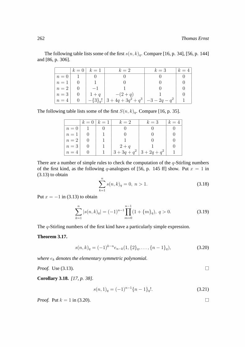
The following table lists some of the firsts(n, k)q. Compare [16, p. 34], [56, p. 144]and [86, p. 306].

k = 0 k = 1 k = 2 k = 3 k = 4n = 0 1 0 0 0 0n = 1 0 1 0 0 0n = 2 0 −1 1 0 0n = 3 0 1 + q −(2 + q) 1 0n = 4 0 −{3}q! 3 + 4q + 3q2 + q3 −3− 2q − q2 1

The following table lists some of the firstS(n, k)q. Compare [16, p. 35].

k = 0 k = 1 k = 2 k = 3 k = 4n = 0 1 0 0 0 0n = 1 0 1 0 0 0n = 2 0 1 1 0 0n = 3 0 1 2 + q 1 0n = 4 0 1 3 + 3q + q2 3 + 2q + q2 1

There are a number of simple rules to check the computation of theq-Stirling numbersof the first kind, as the followingq-analogues of [56, p. 145 ff] show. Putx = 1 in(3.13) to obtain

n∑k=1

s(n, k)q = 0, n > 1. (3.18)

Putx = −1 in (3.13) to obtain

n∑k=1

|s(n, k)q| = (−1)n−1

n−1∏m=0

(1 + {m}q), q > 0. (3.19)

Theq-Stirling numbers of the first kind have a particularly simple expression.

Theorem 3.17.

s(n, k)q = (−1)k−nen−k(1, {2}q, . . . , {n− 1}q), (3.20)

whereek denotes the elementary symmetric polynomial.

Proof. Use (3.13).

Corollary 3.18. [17, p. 38].

s(n, 1)q = (−1)n−1{n− 1}q!. (3.21)

Proof. Putk = 1 in (3.20).


There is an exact formula by Carlitz forS(n, k)q, which will be quite useful.

Theorem 3.19. [17, p. 41 (3.35)], [13, p. 104], [8, p. 990, 3.3], [83, p. 86 13.2](c = 1). A q-analogue of [56, p. 169, (3)], [16, p. 37, 2.31], [82, p. 495], [75, p. 83(19)]. Compare [44, p. 257].

S(n, k)q = ({k}q!q(k2))−1

k∑i=0

(k

i

)q

(−1)iq(i2){k − i}n

q . (3.22)

This formula can also be written as the followingq-analogue of [82].

S(n, k)q =1

{k}q!4n

H,q(x)k,q|x=0. (3.23)

There are a number of simple rules to check the computation of theq-Stirling numbersof the second kind. We start with someq-analogues of Jordan’s book [56, p. 170. f]about finite differences intended both for mathematicians and statisticians.

Theorem 3.20.

(−1)n =n∑

k=0

S(n, k)q(−1)k

k−1∏m=0

(1 + {k}q). (3.24)

Proof. Putx = −1 in (3.14).

Theorem 3.21.S(n + 1, n)q − S(n, n− 1)q = {n}q. (3.25)

Proof. Putk = n in (3.16).

There are two kinds of generating functions forS(n, k)q. The first one is as follows.

Theorem 3.22.[17, p. 42 (3.36)], [61, 7.2.1.5, answer 29], aq-analogue of [56, p. 175(2)], [41, p. 337, 7.47], [83, p. 64, 2.6] and [16, p. 37, 2.30].

∞∑n=m

S(n,m)qtn =

tm

m∏l=1

(1− t{l}q)

, |t| < 1

m. (3.26)

This can be expressed in two other ways. Aq-analogue of [56, p. 193. (1)], whichserves as definition ofq-reciprocal factorial.

∞∑n=m

S(n, m)qz−n−1 =

1

(z)m+1,q

≡ (z)−(m+1),q, z > m. (3.27)

264 Thomas Ernst

A q-analogue of [56, p. 193. (2)] and [16, p. 36, 2.29].

∞∑n=m

S(n, m)q(−x)−n =(−1)m

m∏l=1

(x + {l}q)

, x > m. (3.28)

By the orthogonality relation we obtain aq-analogue of [56, p. 193. (3)].

x−k =∞∑

m=k

|s(m, k)q|m∏

l=1

(x + {l}q)

. (3.29)

The q-Stirling numbers can be used to obtain several exact formulas forq-derivativesandq-integrals as follows.

Theorem 3.23. ∫ 1

0

(t)n,q dq(t) =n∑

k=1

s(n, k)q

{k + 1}q

. (3.30)

Proof. q-integrate (3.13).

Theorem 3.24.A q-analogue of [56, p. 194 (5)].

Dsq

1

(z)m+1,q

=∞∑

n=m

S(n, m)q{−n− s}s,qz−n−1−s. (3.31)

Proof. Use (3.27).

Theorem 3.25.A q-analogue of [56, p. 194 (6)].∫ z 1

(t)m+1,q

dq(t) =∞∑

n=m

S(n, m)q

{−n}qzn+ k. (3.32)

Proof. Use (3.27).

The second generating function forS(n,m)q is as follows.

Theorem 3.26.[17, p. 42 (3.38)]. Aq-analogue of [19, p. 206 (2a)], [83, p. 64, 2.7].

∞∑n=k

S(n, k)qtn

{n}q!= ({k}q!q

(k2))−1

k∑i=0

(k

i

)q

(−1)iq(i2)Eq(t{k − i}q). (3.33)


Proof.

LHS =∞∑

n=k

tn

{n}q!({k}q!q

(k2))−1

k∑i=0

(k

i

)q

(−1)iq(i2){k − i}n

q =

({k}q!q(k2))−1

k∑i=0

(k

i

)q

(−1)iq(i2)

∞∑n=0

(t{k − i}q)n

{n}q!= RHS.

(3.34)

There is a generating function forq-Stirling numbers of the first kind.


n∑k=m

s(n, k)q

(k

m

)qm = qn−1s(n− 1, m)q + qns(n− 1, m− 1)q. (3.35)


Theorem 3.28.A q-analogue of [56, p. 185].

s(n, k)q =n∑

m=k

qn−m−1(−1)m+k

(m

k

)[s(n− 1, m)q + qs(n− 1, m− 1)q]. (3.36)

Corollary 3.29. A q-analogue of [56, p. 186 (4)].

n∑k=1

s(n, k)qk =

{1, n = 1;

qn−2(−1)n{n− 2}q! n > 1.(3.37)

Proof. Putm = 1 in (3.35).

Corollary 3.30. A q-analogue of [56, p. 186 (5)].

m∑n=2

S(m, n)q qn−2(−1)n{n− 2}q! = m− 1. (3.38)

Proof. Applym∑

n=1

S(m, n)q to both sides of (3.37). Then use the orthogonality relation.

The following 3 theorems are proved in exactly the same way as in Jordan [56].


n∑k=1

s(n, k)qS(k + 1, i)q = {n}q

(0

n− i

)+

(0

n + 1− i

). (3.39)

266 Thomas Ernst


n∑k=0

S(n, k)q[s(k + 1, l)q + {k}qs(k, l)q] = δl,n+1. (3.40)


n+1∑k=1

S(n + 1, k)q =n∑

k=1

(1 + {k}q)S(n, k)q, n > 0. (3.41)

The following operator [53] will be useful. In its earliest form withq = 1 it datesback to Euler and Abel [1, B. 2, p. 41], who used it in differential equations.

Definition 3.34.θq ≡ xDq. (3.42)

Theorem 3.35.Cigler [17, p. 37 (3.8)]. Aq-analogue of the Grunert operator formula[44, 247], [39, p. 455, 4.8], [78, p. 181], [83, p. 64, 2.1], [75, p. 81, (2)], [56, p. 196(2)], [63, p. 95].

θnq =

n∑k=0

S(n, k)q q(k2)xkDk

q . (3.43)

Proof. Induction.

This leads to the following inverse formula.

Theorem 3.36.Cigler [17, p. 37 (3.9)]. Aq-analogue of [80, p 548], [78, p 183].

q(n2)xnDn

q =n∑

k=1

s(n, k)qθkq . (3.44)

Proof. Use the orthogonality relation forq-Stirling numbers.

The previous formula can be expressed in another way.

Theorem 3.37.Jackson [52, p. 305]. Aq-analogue of the 1844 Boole formula [5], [78,p 183], [12, p 24, (2.1)].

q(n2)xnDn

q =n−1∏k=0

(θq − {k}q). (3.45)

Proof. Use (3.13).


Example 3.38.A q-analogue of [56, p. 196]. Letf(x) = (x⊕q 1)n and apply (3.43) toget

n∑k=0

(n

k

)q

xk{k}mq =

min(m,n)∑k=0

S(m, k)q q(k2)xk{n− k + 1}k,q(x⊕q 1)n−k. (3.46)

Putx = 1 to get

n∑k=0

(n

k

)q

{k}mq =

min(m,n)∑k=0

S(m, k)q q(k2){n− k + 1}k,q(1⊕q 1)n−k. (3.47)

If we put m = 1 or m = 2 in (3.47), we getq-analogues of the mean and variance ofthe binomial distribution from Melzak [63, p. 96].

Putx = −1 in (3.46) to get

n∑k=0

(n

k

)q

(−1)k{k}mq =

min(m,n)∑k=0

S(m, k)q q(k2)(−1)k{n−k+1}k,q(1q1)n−k. (3.48)

Example 3.39.Let f(x) = (x �q 1)n and apply (3.43) to get

n∑k=0

(n

k

)q

q(k2) xn−k{n− k}m

q =

min(m,n)∑k=0

S(m, k)q q(k2)xk{n− k + 1}k,q(x �q 1)n−k.

(3.49)Putx = 1 to get

n∑k=0

(n

k

)q

q(k2) {n− k}m

q =

min(m,n)∑k=0

S(m, k)q q(k2){n− k + 1}k,q(1 �q 1)n−k. (3.50)

Putx = −1 to get (3.22).

Theorem 3.40.A q-analogue of Cauchy [10, p. 161].

Dmq (Eq(αx)f(x)) = Eq(αx)(Dq ⊕q αε)mf(x). (3.51)

We continue with a few equations with operator proofs in the spirit of Gould andSchwatt.

Theorem 3.41.Almost aq-analogue of [39, p 455, 4.9].

n∑k=0

{k}qpxk =

p∑k=0

S(p, k)q q(k2)xkDk

q

(xn+1 − 1

x− 1

). (3.52)

We obtain the following limit.

268 Thomas Ernst

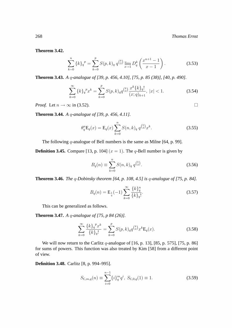
Theorem 3.42.

n∑k=0

{k}qp =

p∑k=0

S(p, k)q q(k2) lim

x→1Dk

q

(xn+1 − 1

x− 1

). (3.53)

Theorem 3.43.A q-analogue of [39, p. 456, 4.10], [75, p. 85 (38)], [40, p. 490].

∞∑k=0

{k}qpxk =

p∑k=0

S(p, k)qq(k2) xk{k}q!

(x; q)k+1

, |x| < 1. (3.54)

Proof. Let n →∞ in (3.52).

Theorem 3.44.A q-analogue of [39, p. 456, 4.11].

θnq Eq(x) = Eq(x)

n∑k=0

S(n, k)q q(k2)xk. (3.55)

The followingq-analogue of Bell numbers is the same as Milne [64, p. 99].

Definition 3.45. Compare [13, p. 104](x = 1). Theq-Bell number is given by

Bq(n) ≡n∑

k=0

S(n, k)q q(k2). (3.56)

Theorem 3.46.Theq-Dobinsky theorem [64, p. 108, 4.5] isq-analogue of [75, p. 84].

Bq(n) = E1q(−1)

∞∑k=0

{k}nq

{k}q!. (3.57)

This can be generalized as follows.

Theorem 3.47.A q-analogue of [75, p 84 (26)].

∞∑k=0

{k}qpxk

{k}q!=

p∑k=0

S(p, k)qq(k2)xkEq(x). (3.58)

We will now return to the Carlitzq-analogue of [16, p. 13], [85, p. 575], [75, p. 86]for sums of powers. This function was also treated by Kim [58] from a different pointof view.

Definition 3.48. Carlitz [8, p. 994–995].

SC,m,q(n) ≡n−1∑i=0

{i}mq qi, SC,0,q(1) ≡ 1. (3.59)


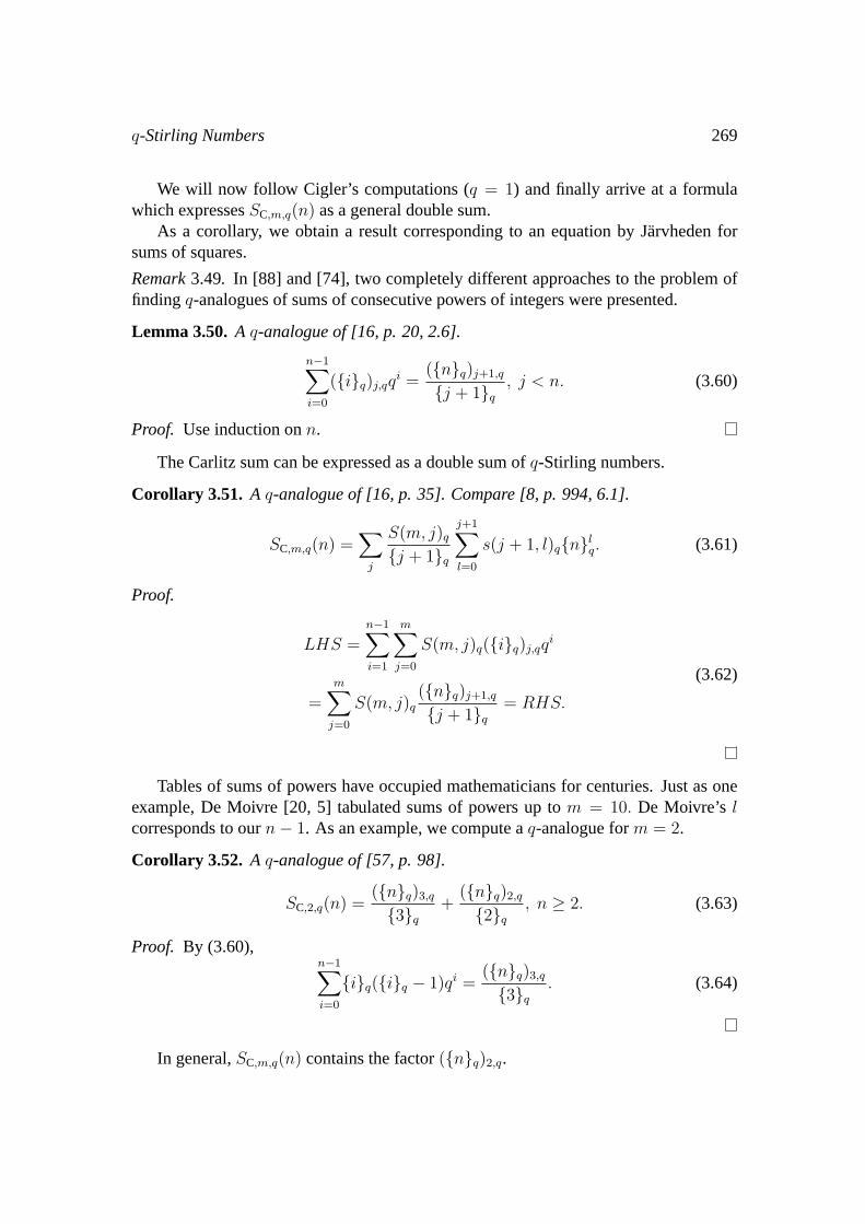
We will now follow Cigler’s computations (q = 1) and finally arrive at a formulawhich expressesSC,m,q(n) as a general double sum.

As a corollary, we obtain a result corresponding to an equation by Jarvheden forsums of squares.

Remark3.49. In [88] and [74], two completely different approaches to the problem offinding q-analogues of sums of consecutive powers of integers were presented.

Lemma 3.50.A q-analogue of [16, p. 20, 2.6].

n−1∑i=0

({i}q)j,qqi =

({n}q)j+1,q

{j + 1}q

, j < n. (3.60)

Proof. Use induction onn.

The Carlitz sum can be expressed as a double sum ofq-Stirling numbers.

Corollary 3.51. A q-analogue of [16, p. 35]. Compare [8, p. 994, 6.1].

SC,m,q(n) =∑

j

S(m, j)q

{j + 1}q

j+1∑l=0

s(j + 1, l)q{n}lq. (3.61)

Proof.

LHS =n−1∑i=1

m∑j=0

S(m, j)q({i}q)j,qqi

=m∑

j=0

S(m, j)q({n}q)j+1,q

{j + 1}q

= RHS.

(3.62)

Tables of sums of powers have occupied mathematicians for centuries. Just as oneexample, De Moivre [20, 5] tabulated sums of powers up tom = 10. De Moivre’s lcorresponds to ourn− 1. As an example, we compute aq-analogue form = 2.

Corollary 3.52. A q-analogue of [57, p. 98].

SC,2,q(n) =({n}q)3,q

{3}q

+({n}q)2,q

{2}q

, n ≥ 2. (3.63)

Proof. By (3.60),n−1∑i=0

{i}q({i}q − 1)qi =({n}q)3,q

{3}q

. (3.64)

In general,SC,m,q(n) contains the factor({n}q)2,q.

270 Thomas Ernst

4 The Carlitz–Gould Approach

The following operators were introduced by Carlitz [8, p. 988] 1948. Schendel [73],Gould [36], Milne [64], Zeng [90] and Phillips [69] used the same technique. Ap-plications from approximation theory can be found in Phillips [69]. Observe that the

q-Stirling number of the second kind used by Milne [64, p. 93] isq(k2)S(n, k)q.

Definition 4.1. The Carlitz–Gouldq-difference is defined by

41CG,qf(x) ≡ f(x + 1)− f(x), 4n+1

CG,qf(x) ≡ 4nCG,qf(x + 1)− qn4n

CG,qf(x). (4.1)

Remark4.2. We get the above definition by puttingy = −1 in Schendel [73].

Now follow the Carlitz–Gould quartet and two examples.

Theorem 4.3.The followingq-Taylor formula applies [8, 2.5 p. 988], [38, 7.2, p. 856],[36, 2.11, p. 91].

f(x) =∞∑

k=0

4kCG,qf(0)

{k}q!{x− k + 1}k,q. (4.2)

Proof. Apply 4sCG,q to both members and finally putx = 0.

Theorem 4.4. [37, p. 283, 2.13], [90], [36, 2.10, p. 91], [69, p. 46, 1.118], [64, p. 91]and aq-analogue of [16, p. 26]. Compare [73, p. 82].

4nCG,qf(x) =

n∑k=0

(−1)k

(n

k

)q

q(k2)En−kf(x), (4.3)

where the shift operatorE is given by

Enf(x) ≡ f(x + n). (4.4)

Proof. Use induction.


Theorem 4.5.

Enf(x) =n∑

i=0

(n

i

)q

4iCG,qf(x). (4.5)

Proof. This is the general inversion formula again, compare the corrected version of [34,p. 244].

Corollary 4.6. [69, p. 47 1.122], aq-analogue of [56, p. 97, 10], [16, p. 27, 2.13], [65,p. 35, 2]. Assume that the functionsf(x) andg(x) depend onqx. Then

4nCG,q(fg) =

n∑i=0

(n

i

)q

4iCG,qf4n−i

CG,qEig. (4.6)


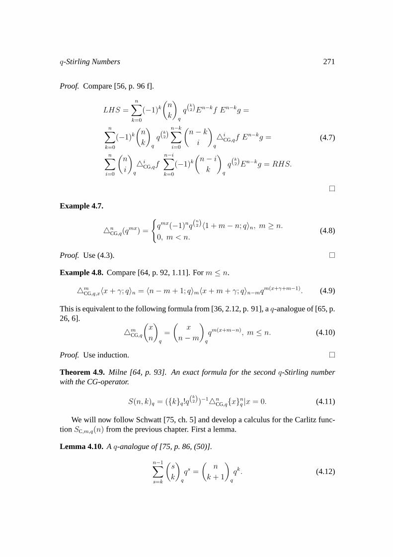
Proof. Compare [56, p. 96 f].

LHS =n∑

k=0

(−1)k

(n

k

)q

q(k2)En−kf En−kg =

n∑k=0

(−1)k

(n

k

)q

q(k2)

n−k∑i=0

(n− k

i

)q

4iCG,qf En−kg =

n∑i=0

(n

i

)q

4iCG,qf

n−i∑k=0

(−1)k

(n− i

k

)q

q(k2)En−kg = RHS.

(4.7)

Example 4.7.

4nCG,q(q

mx) =

{qmx(−1)nq(

n2)〈1 + m− n; q〉n, m ≥ n.

0, m < n.(4.8)

Proof. Use (4.3).

Example 4.8.Compare [64, p. 92, 1.11]. Form ≤ n.

4mCG,q,x〈x + γ; q〉n = 〈n−m + 1; q〉m〈x + m + γ; q〉n−mqm(x+γ+m−1). (4.9)

This is equivalent to the following formula from [36, 2.12, p. 91], aq-analogue of [65, p.26, 6].

4mCG,q

(x

n

)q

=

(x

n−m

)q

qm(x+m−n), m ≤ n. (4.10)

Proof. Use induction.

Theorem 4.9. Milne [64, p. 93]. An exact formula for the secondq-Stirling numberwith the CG-operator.

S(n, k)q = ({k}q!q(k2))−14n

CG,q{x}nq |x = 0. (4.11)

We will now follow Schwatt [75, ch. 5] and develop a calculus for the Carlitz func-tion SC,m,q(n) from the previous chapter. First a lemma.

Lemma 4.10.A q-analogue of [75, p. 86, (50)].

n−1∑s=k

(s

k

)q

qs =

(n

k + 1

)q

qk. (4.12)

272 Thomas Ernst

Theorem 4.11.A q-analogue of [75, p. 86, (51)].

SC,m,q(n) =m∑

k=0

(−1)kqk

(n

k + 1

)q

k∑a=0

(−1)a

(k

a

)q

q(k−a

2 ){a}mq . (4.13)

Proof. Write the LHS as

θmq

n−1∑k=1

(xq)k|x=1, (4.14)

and use (3.43), (4.12) and (3.22).


SC,m,q(n) =n∑

k=0

(n

k

)q

k∑a=0

(−1)a

(k

a

)q

q(a2)

k−a−1∑i=1

{i}mq qi. (4.15)

Proof. Use (4.2) and (4.3).

Now let bm,k,q denote the coefficient ofqk

(n

k + 1

)q

in SC,m,q(n). Then by (4.13)

we obtain the following recurrence, which is almost aq-analogue of [75, p. 88 (69)].

bm,k,q − {k}qbm−1,k,q = qk−1{k}qbm−1,k−1,q. (4.16)

We obtain the following expressions forSC,m,q(n) expressed as linear combinations ofq-binomial coefficients.

Theorem 4.13.Almost aq-analogue of Schwatt [75, p. 88 (69)].

SC,1,q(n) = q

(n

2

)q

. (4.17)

SC,2,q(n) = q

(n

2

)q

+ q3(1 + q)

(n

3

)q

. (4.18)

SC,3,q(n) = q

(n

2

)q

+ q3(1 + q + (1 + q)2)

(n

3

)q

+

q6(1 + q)(1 + q + q2)

(n

4

)q

.

(4.19)

SC,4,q(n) = q

(n

2

)q

+ q3(1 + q)(2 + q + (1 + q)2)

(n

3

)q

+ q6(1 + q + q2)

× (1 + q + (1 + q)2 + {3}q!)

(n

4

)q

+ q10{4}q!

(n

5

)q

.

(4.20)


By theq-Pascal identity we obtain the followingq-analogue of Munch [66, p. 14].

Theorem 4.14.

SC,2,q(n) = q3

(n

3

)q

+ q

(n + 1

3

)q

. (4.21)

SC,3,q(n) = q6

(n

4

)q

+ 2q3(1 + q)

(n + 1

4

)q

+ q

(n + 2

4

)q

. (4.22)

SC,4,q(n) = q10

(n

5

)q

+ q6(3 + 5q + 3q2)

(n + 1

5

)q

+

+ q3(3 + 5q + 3q2)

(n + 2

5

)q

+ q

(n + 3

5

)q

.

(4.23)

We can now introduce the sum operator mentioned in the introduction.

Definition 4.15. The inverse CG difference is defined by

4−1CG,qf(k)|n0 ≡

n∑0

f(x)δq(x) ≡n−1∑k=0

f(k). (4.24)

Example 4.16.

4−1CG,q(1− ql)〈n + 1; q〉l−1 qn ≡

n−1∑k=0

(1− ql)〈k + 1; q〉l−1qk = 〈n; q〉l. (4.25)

Corollary 4.17.

{n}q{n + 1}q = {2}q

n∑i=1

{i}qqi−1. (4.26)

n∑i=1

{i}qq2i =

{n}2,q

{2}q

− {n}3,q(1− q)

{3}q

. (4.27)

It is possible to develop a calculus similar toSC,m,q(n) for the sum (4.27), but wehave not pursued this path.

By (4.3) and (4.9) we obtain the following.

Theorem 4.18.[67, p. 110].

m∑n=0

(−1)n

(m

n

)q

q(n2)〈x + 1; q〉m−n〈x− y + 1− n + m; q〉n =

〈y −m + 1; q〉mqm(x−y+m), x, y ∈ C.

(4.28)

We will return to this equation in the next chapter. Now we say goodbye to theCarlitz–Gould approach and continue with a similar operator which has the advantageof being both aq-derivative and difference operator at the same time.

274 Thomas Ernst

5 The Jacksonq-derivative as Difference Operator

This chapter will be about how the Jacksonq-derivative can be used as difference oper-ator operating on the space of allq-shifted factorials. We illustrate the technique withsome examples. The similarity with the operator from the previous chapter is strikingand will apparently lead to many multipleq-equations. However it turns out that mostof these are doublets, as is shown in the example from the last chapter.

For functions ofqx, the Cigler operatorε [13] will be replaced byE in q-Leibniztheorems as below.

Theorem 5.1.

Dnq,qx〈γ + x; q〉k = (−1)n{k − n + 1}n,q〈γ + x + n; q〉k−nq

(n2)+nγ, n ≤ k. (5.1)

Example 5.2.We apply the operatorDmq,qx to (4.28). Then

LHS =m∑

n=0

(−1)n

(m

n

)q

q(n2)

m∑i=0

(m

i

)q

Diq,qx〈x + 1; q〉m−n

EiDm−iq,qx 〈x− y + 1− n + m; q〉n =

m∑n=0

(−1)n

(m

n

)q

q(n2)×(

m

m− n

)q

(−1)m{m− n}q!q(m−n

2 )+m−n{n}q! q(n2)+n(−y+1−n+m)

= (−1)mq(m2 )+m{m}q!

m∑n=0

(−1)n

(m

n

)q

q(n2)−ny =

qm2−my〈y + 1−m; q〉m{m}q! = RHS.

(5.2)

Now instead rewrite (4.28) in the formm∑

n=0

(m

n

)q

〈x + 1; q〉m−n〈y − x−m; q〉nqn(x+m)+y(m−n) =

〈y −m + 1; q〉mqm(x+m), x, y ∈ C,

(5.3)

and operate withDmq,qy on both sides to obtain

LHS =m∑

n=0

(m

n

)q

〈x + 1; q〉m−nqn(x+m)

m∑i=0

(m

i

)q

Diq,qyqy(m−n)

EiDm−iq,qy 〈y − x−m; q〉n =

m∑n=0

(m

n

)q

〈x + 1; q〉m−nqn(x+m)×(

m

m− n

)q

{m− n}q!(−1)n{n}q!q(n

2)−n(x+m)

= {m}q!m∑

n=0

(m

n

)q

〈x + 1; q〉m−n(−1)nq(n2).

(5.4)


The RHS is(−1)m{m}q!q

(m2 )+m(x+1). (5.5)

After simplification this last equality is equivalent to a confluent form of the secondq-Vandermonde identity.

Inspired by the previous calculation we make the following definition.

Definition 5.3. The Jacksonq-difference is defined by

4J,x,qf(qx) ≡ 4J,qf(qx)

≡ (f(qx+1)− f(qx))q−x ≡ −(1− q)Dq,qxf(qx),(5.6)

4n+1J,q = 4J,q4n

J,q. (5.7)

The following equation is obtained.

Theorem 5.4.

4J,q

(q(

k2)(

x

k

)q

)= q(

k−12 )(

x

k − 1

)q

. (5.8)

Proof. Use theq-Pascal identity.

Corollary 5.5.

4mJ,q

(x

n

)q

=

(x

n−m

)q

q−mn+(m+12 ), m ≤ n. (5.9)

Example 5.6.∞∑

n=0

q(n2)(

x

n

)q

tn = eq(−tqx �q t). (5.10)

Proof. Use theq-binomial theorem.

We now present the Jackson quartet.

Theorem 5.7.The followingq-Taylor formula applies.

f(x) =∞∑

k=0

(x

k

)q

q(k2)4k

J,qf(0). (5.11)

Theorem 5.8.A q-analogue of [16, p. 26]. Compare [73, p. 82].

4nJ,qf(qx) = q−nx−(n

2)n∑

k=0

(−1)k

(n

k

)q

q(k2)En−kf(qx). (5.12)

Proof. Use the corresponding equation for theq-derivative.

276 Thomas Ernst


Theorem 5.9.

Enf(qx) =n∑

k=0

qxk+(k2)(

n

k

)q

4kJ,qf(qx). (5.13)

Corollary 5.10. A q-analogue of [56, p. 97, 10], [16, p. 27, 2.13], [65, p. 35, 2].

4nJ,q(f(qx)g(qx)) =

n∑k=0

(n

k

)q

4kJ,qf(qx)(4n−k

J,q Ek)g(qx). (5.14)

Proof. Use the Leibniz theorem for theq-derivative.

Example 5.11.

4nJ,q(q

mx) =

{qx(m−n)(−1)n〈1 + m− n; q〉n, m ≥ n.

0, m < n.(5.15)

6 Applications

The developed technique leads to easy proofs ofq-binomial coefficient identities. Thefollowing example can also be proved from theq-Vandermonde identity.

Example 6.1.A q-analogue of the important formula [16, p. 27], [70, p. 15, (9)], [71, p.65]. (

x

m

)q

(x

n

)q

=m+n∑k=0

QE((k − n)(k −m))×(k

n

)q

(n

m + n− k

)q

(x

k

)q

.

(6.1)

Proof. We have

4kCG,q

(x

m

)q

(x

n

)q

=k∑

l=0

(k

l

)q

QE(l(x + l − n) + (k − l)(x + k −m))×(x + l

m− k + l

)q

(x

n− l

)q

.

(6.2)

Now use theq-Taylor formula (4.2) withy = 0, f(x) =

(x

m

)q

(x

n

)q

.


Remark6.2. If we use4J,q instead, we get(x

m

)q

(x

n

)q

=m+n∑k=0

QE

(−(

m

2

)−(

n

2

)+

(m + n− k

2

)+

(k

2

))×(

k

n

)q

(n

m + n− k

)q

(x

k

)q

.

(6.3)

This equation is however equivalent to (6.1).

Acknowledgments. I would like to thank Don Knuth and Johann Cigler for theirkind advice. Karl Dilcher’s Bernoulli bibliography has also been an invaluable help.Several computations have been checked byMathematica.

References

[1] N.H. Abel, OEuvres completes de Niels Henrik AbelChristiana: Imprimerie deGrondahl and Son; New York and London: Johnson Reprint Corporation. VIII,621 p. (1965).

[2] L. Aceto, and D. Trigiante, The matrices of Pascal and other greats.Amer. Math.Monthly108 (2001), no. 3, 232–245.

[3] M. Aigner, Combinatorial theory. Grundlehren der Mathematischen Wissen-schaften 234. Springer-Verlag, Berlin-New York, 1979.

[4] E.G. Bjorling, In determinationem coefficientium . . .Crelle J. 28. (1844), 284–288.

[5] G. Boole, On a general method in analysis.Philosophical transactions, 134, 225–282 (1844).

[6] G. Boole,A treatise on the calculus of finite differences. 2nd ed. 1872.

[7] F. Cajori,A History of Mathematical Notations. V2. Chicago 1929.

[8] L. Carlitz, q-Bernoulli numbers and polynomials.Duke math. J.15 (1948), 987–1000.

[9] L. Carlitz, Stirling pairs.Rend. Sem. Mat. Univ. Padova59 (1978), 19–44.

[10] A. Cauchy, Exercices de mathematique, seconde annee. Paris 1827.

[11] A. Cayley, Table of∆m0n ÷Π(m) up tom = n = 20. Cambr. Trans. XIII. 1–4.(1881)

278 Thomas Ernst

[12] S.K. Chatterjea, Operational formulae for certain classical polynomials. I.Quart.J. Math. OxfordSer. (2) 14 (1963), 241–246.

[13] J. Cigler, Operatormethoden fur q-Identitaten.Monatshefte fur Math. 88,(1979),87–105.

[14] J. Cigler, Operatormethoden fur q-Identitaten II: q-Laguerre-Polynome.Monat-shefte fur Math.91,(1981) 105–117.

[15] J. Cigler, A characterisation of theq-exponential polynomials. (Eine Charakter-isierung derq-Exponentialpolynome.)Sitzungsber., Abt. II, sterr. Akad. Wiss.,Math.-Naturwiss. Kl. 208, 143–157 (1999).

[16] J. Cigler,Differenzenrechnung. Wien 2001.

[17] J. Cigler,Elementareq-IdentitatenSkriptum Wien 2006

[18] D. Crippa, and K. Simon, and P. Trunz, Markov processes involvingq-Stirlingnumbers.Comb. Probab. Comput.6, No.2, 165–178 (1997)

[19] L. Comtet,Advanced combinatorics. Reidel 1974.

[20] A. De Moivre,Miscellanea Analytica. London 1730.

[21] A. De Morgan,The differential and integral CalculusBaldwin and Cradock, Lon-don 1842. Elibron Classics, 2002.

[22] T. Ernst,The history ofq-calculus and a new method,Uppsala 2000.

[23] T. Ernst,q-Generating functions for one and two variables.Simon Stevin, 12 no.4, 2005, 589–605.

[24] T. Ernst,A new method forq-calculus,Uppsala dissertations 2002.

[25] T. Ernst, A method forq-calculus.J. nonlinear Math. Physics10 No.4 (2003),487–525.

[26] T. Ernst, Some results forq-functions of many variables.Rendiconti di Pado-va,112(2004), 199–235.

[27] T. Ernst,q-Analogues of some operational formulas. Preprint 2003.

[28] T. Ernst,q-Bernoulli andq-Euler Polynomials, An Umbral Approach.Interna-tional journal of difference equations1 no. 1 2006, 13–62.

[29] L. Euler,Institutiones calculi differentialis1755, new printing Birkhuser 1913.

[30] C-E. Froberg,Larobok i numerisk analys. Stockholm 1962.


[31] G. Gasper, and M. Rahman,Basic hypergeometric series,Cambridge, 1990.

[32] C.F. Gauss,Werke 2. 1876, 9–45.

[33] I.M. Gelfand, and M.I. Graev, and V.S. Retakh, General hypergeometric systemsof equations and series of hypergeometric type. (Russian)Uspekhi Mat. Nauk47(1992), no. 4, (286),3–82, 235, translation inRussian Math. Surveys47 (1992),no. 4 1–88.

[34] J. Goldman, and G.C. Rota, On the foundations of combinatorial theory. IV. Finitevector spaces and Eulerian generating functions.Stud. Appl. Math.49 (1970),239–258.

[35] H.H. Goldstine,A history of numerical analysis from the 16th through the 19thcentury. Studies in the History of Mathematics and Physical Sciences, Vol. 2.Springer 1977.

[36] H.W. Gould, Theq-series generalization of a formula of Sparre Andersen.Math.Scand. 9 (1961), 90–94.

[37] H.W. Gould, Theq-Stirling numbers of first and second kinds.Duke Math. J. 28(1961), 281–289.

[38] H.W. Gould, The operator(ax∆)n and Stirling numbers of the first kind.Amer.Math. Monthly71 (1964), 850–858.

[39] H.W. Gould, Euler’s formula forn-th differences of powers.Am. Math. Mon. 85,450–467 (1978).

[40] H.W. Gould, Evaluation of sums of convolved powers using Stirling and Euleriannumbers.The Fibonacci quarterly16, 6 (1978), 488–497.

[41] R.L. Graham, and D.E. Knuth, and O. Patashnik,Concrete mathematics. A foun-dation for computer science. Second edition. Addison-Wesley Publishing Com-pany, Reading, MA, 1994.

[42] J.A. Grunert, Math. Abhandlungen, Erste Sammlung, Altona: Hammerich 1822.

[43] J.A. Grunert, Summierung der Reihe...Borchardt J.2. (1827), 358–363.

[44] J.A. Grunert,Uber die Summierung der Reihen von der Form . . .Borchardt J. 25.(1843), 240–279.

[45] C. Gudermann,Grundriss der analytischen Spharik. Koln 1830.

[46] C. Gudermann,Potenzial oder cyklisch-hyperbolische Functionen. Berlin 1833.

280 Thomas Ernst

[47] W. Hahn, Uber Orthogonalpolynome, dieq-Differenzengleichungen genugen.Mathematische Nachrichten2 (1949), 4–34.

[48] E. Heine,Uber die Reihe...J. reine angew. Math. 32, (1846) 210–212.

[49] J. Herschel,Collection of examples of the applications of calculus of finite differ-ences.Cambridge 1820.

[50] C.F. Hindenburg,Archiv der reinen und angewandten Mathematik. Leipzig, 1795.

[51] C.F. Hindenburg,Uber combinatorische Analysis und Derivations-calcul. Leip-zig 1803.

[52] F.H. Jackson, Onq-difference equations.American J. Math.32 (1910), 305–314.

[53] F.H. Jackson, On basic double hypergeometric functions.Quart. J. Math.13(1942) 69–82.

[54] W.P. Johnson, Some applications of theq-exponential formula.Proceedings ofthe 6th Conference on Formal Power Series and Algebraic Combinatorics(NewBrunswick, NJ, 1994).Discrete Math. 157(1996), no. 1-3, 207–225.

[55] Ch. Jordan,Statistique mathematique. Paris, Gauthier–Villars. (1927)

[56] Ch. Jordan,Calculus of finite differences. Third Edition. Chelsea Publishing Co.,New York 1950.

[57] B. Jarvheden,Elementar kombinatorikStudentlitteratur 1976.

[58] T. Kim, Sums of powers of consecutiveq-integers. Adv. Stud. Contemp. Math.(Kyungshang)9 (2004), no. 1, 15–18.

[59] F. Klein, Vorlesungen ber die Entwickelung der Mathematik im 19. Jahrhundert.Bd. I+II. Bearbeitet von R. Courant und St. Cohn–Vossen. Springer 1979.

[60] D. Knuth, Two notes on notation.Am. Math. Mon. 99, No.5, 403–422 (1992).

[61] D. Knuth,The Art of Computer Programming, Volume 4, to be published 2005.

[62] B.A. Kupershmidt,q-Newton binomial: from Euler to Gauss.J. Nonlinear Math.Phys.7 (2000), no. 2, 244–262. 123–140.

[63] Z.A. Melzak, Companion to concrete mathematics, vol. 1. Mathematical tech-niques and various applications. Pure and Applied Mathematics. John Wiley &Sons, New York-London-Sydney, 1973.

[64] S.C. Milne, q-analog of restricted growth functions, Dobinski’s equality, andCharlier polynomials.Trans. Amer. Math. Soc. 245(1978), 89–118.


[65] L.M. Milne-Thomson,The Calculus of Finite Differences. Macmillan and Co.,Ltd., London, 1951.

[66] O.J. Munch, On power product sums.Nordisk Mat. Tidskr. 7 (1959), 5–19.

[67] M. Nishizawa, Evaluation of a certainq-determinant.Linear Algebra Appl.342(2002), 107–115.

[68] N.E. Norlund, Memoire sur les polynomes de Bernoulli.Acta Math. 43 (1920),121–196.

[69] G.M. Phillips, Interpolation and approximation by polynomials.CMS Books inMathematics/Ouvrages de Mathematiques de la SMC,14. Springer-Verlag, NewYork, 2003.

[70] J. Riordan,Combinatorial identities. Reprint of the 1968 original. Robert E.Krieger Publishing Co., Huntington, N.Y., 1979.

[71] Finite operator calculus. Edited by Gian-Carlo Rota. With the collaboration of P.Doubilet, C. Greene, D. Kahaner, A. Odlyzko and R. Stanley. Academic Press,Inc. [Harcourt Brace Jovanovich, Publishers], New York-London, 1975.

[72] L. Saalschutz, Vorlesungenuber die Bernoulli’schen Zahlen, ihren Zusammen-hang mit den Secanten-Coefficienten und ihre wichtigeren Anwendungen. Berlin.J. Springer. VIII + 208 S.8◦. (1893)

[73] L. Schendel, Zur Theorie der Functionen. (x)Borchardt J. LXXXIV . 80–84.(1877)

[74] M. Schlosser,q-analogues of the sums of consecutive integers, squares, cubes,quarts and quints.Electron. J. Combin. 11 (2004), no. 1

[75] I.J. Schwatt,An introduction to the operations with series. Philadelphia: ThePress of the University ol Pennsylvannia, 1924.

[76] D.B. Sears, On the transformation theory of basic hypergeometric functions. (En-glish)Proc. London Math. Soc (2)53, (1951) 158–180.

[77] A. Sharma, and A.M. Chak, The basic analogue of a class of polynomials.Riv.Mat. Univ. Parma5 (1954), 325–337.

[78] E. Stephens,The elementary theory of operational mathematics. McGraw-Hill(1937).

[79] J. Stirling,Methodus differentialis. London, 1730.

282 Thomas Ernst

[80] L. Toscano, Sull’iterazione degli operatorixD eDx. (On integration of the oper-atorsxD andDx). [J] Ist. Lombardo, Rend., II. Ser.67, 543–551 (1934).

[81] L. Toscano, Differenze finite e derivate dei polinomi di Iacobi. (Italian)Matem-atiche, Catania10 (1955), 44–56.

[82] L. Toscano, Numeri di Stirling generalizzati e operatori permutabili di secondoordine. (Italian)Matematiche(Catania)24 (1969), 492–518.

[83] L. Toscano, L’operatorexD e i numeri di Bernoulli e di Eulero. (Italian)Matem-atiche31(1976), 63–89 (1977).

[84] A.T. Vandermonde,Histoire de l’Academie Royale des Sciences1772, p. 489–498.

[85] H.S. Vandiver, Simple explicit expressions for generalized Bernoulli numbers ofthe first order.Duke Math. J. 8 (1941), 575–584.

[86] R. Vein and P. Dale,Determinants and their applications in mathematicalphysics. Applied Mathematical Sciences, 134. Springer-Verlag, New York, 1999.

[87] M. Ward, A calculus of sequences.Amer. J. Math.58 (1936), 255–266.

[88] O. Warnaar,Electron. J. Combin.11 (2004).

[89] J. Worpitzky, Studienuber die Bernoullischen und Eulerschen Zahlen.J. f. Math.94 (1883), 203–232.

[90] J. Zeng, Theq-Stirling numbers, continued fractions and theq-Charlier andq-Laguerre polynomials.J. Comput. Appl. Math. 57 (1995), no. 3, 413–424.

q-stirling numbers, an umbral approachcampus.mst.edu/adsa/contents/v3n2p4.pdf · stirling numbers...

Documents