python for computational science and engineering slides
DESCRIPTION
Python Computational SlidesTRANSCRIPT
Computational Science and Engineering in
Python
Hans Fangohr
Engineering and the EnvironmentUniversity of Southampton
United [email protected]
September 23, 2014
1 / 334

Outline I1 Python prompt
2 Functions
3 About Python
4 Coding style
5 Conditionals, if-else
6 Sequences
7 Loops
8 Some things revisited
9 File IO
10 Exceptions
11 Printing
12 Higher Order Functions
13 Modules
14 Default arguments
15 Namespaces
16 Python IDEs
17 List comprehension
18 Dictionaries2 / 334

Outline II19 Recursion
20 Common Computational Tasks
21 Root finding
22 Derivatives
23 Numpy
24 Higher Order Functions 2: Functional tools
25 Object Orientation and all that
26 Numerical Integration
27 Numpy usage examples
28 Scientific Python
29 ODEs
30 Sympy
31 Testing
32 Some programming languages
33 What language to learn next?
3 / 334

First steps with the Pythonprompt
4 / 334

The Python prompt
Spyder (or IDLE, or python or python.exe fromshell/Terminal/MS-Dos prompt, or IPython)
Python prompt waits for input:
>>>
Interactive Python prompt waits for input:
In [1]:
Read, Evaluate, Print, Loop → REPL
5 / 334

Hello World program
Standard greeting:
print("Hello World!")
Entered interactively in Python prompt:
>>> print("Hello World!")
Hello World!
Or in IPython prompt:
In [1]: print("Hello world")
Hello world
6 / 334

A calculator
>>> 2 + 3
5
>>> 42 - 15.3
26.7
>>> 100 * 11
1100
>>> 2400 / 20
120
>>> 2 ** 3 # 2 to the power of 3
8
>>> 9 ** 0.5 # sqrt of 9
3.0
7 / 334
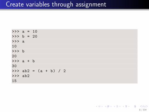
Create variables through assignment
>>> a = 10
>>> b = 20
>>> a
10
>>> b
20
>>> a + b
30
>>> ab2 = (a + b) / 2
>>> ab2
15
8 / 334

Important data types / type()
>>> a = 1
>>> type(a)
<type ’int’> # integer
>>> b = 1.0
>>> type(b)
<type ’float’> # float
>>> c = ’1.0’
>>> type(c)
<type ’str’> # string
>>> d = 1 + 3j
>>> type(d)
<type ’complex ’> # complex number
9 / 334

Beware of integer division
This is the problem:
>>> 1 / 2
0 # expected 0.5, not 0
Solution: change (at least) one of the integer numbers into afloating point number (i.e. 1 → 1.0).
>>> 1.0 / 2
0.5
>>> 1 / 2.0
0.5
10 / 334

Summary useful commands (introspection)
print(x) to display the object x
type(x) to determine the type of object x
help(x) to obtain the documentation string
dir(x) to display the methods and members of object x,or the current name space (dir()).
Example:
>>> help("abs")
Help on built -in function abs:
abs (...)
abs(number) -> number
Return the absolute value of the argument.
11 / 334

Interactive documentation, introspection
>>> word = ’test’
>>> print(word)
test
>>> type(word)
<type ’str’>
>>> dir(word)
[’__add__ ’, ’__class__ ’, ’__contains__ ’, ...,
’__doc__ ’, ..., ’capitalize ’, <snip >,
’endswith ’, ..., ’upper’, ’zfill’]
>>> word.upper()
’TEST’
>>> word.capitalize ()
’Test’
>>> word.endswith(’st’)
True
>>> word.endswith(’a’)
False
12 / 334

Functions
13 / 334

First use of functions
Example 1:
def mysum(a, b):
return a + b
#main program starts here
print "The sum of 3 and 4 is", mysum(3, 4)
14 / 334
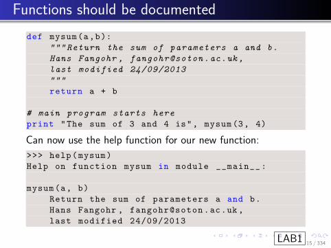
Functions should be documented
def mysum(a,b):
""" Return the sum of parameters a and b.
Hans Fangohr , [email protected] ,
last modified 24/09/2013
"""
return a + b
# main program starts here
print "The sum of 3 and 4 is", mysum(3, 4)
Can now use the help function for our new function:
>>> help(mysum)
Help on function mysum in module __main__:
mysum(a, b)
Return the sum of parameters a and b.
Hans Fangohr , [email protected] ,
last modified 24/09/2013
LAB115 / 334

Function terminology
x = -1.5
y = abs(x)
x is the argument given to the function
y is the return value (the result of the function’scomputation)
Functions may expect zero, one or more arguments
Not all functions (seem to) return a value. (If no return
keyword is used, the special object None is returned.)
16 / 334

Function example
def plus42(n):
""" Add 42 to n and return """ # docstring
l = n + 42 # body of
# function
return l
a = 8
b = plus42(a) # not part of function definition
After execution, b carries the value 50 (and a = 8).
17 / 334

Summary functions
Functions provide (black boxes of) functionality: crucialbuilding blocks that hide complexity
interaction (input, output) through input arguments andreturn values (printing and returning values is not thesame!)
docstring provides the specification (contract) of thefunction’s input, output and behaviour
a function should (normally) not modify input arguments(watch out for lists, dicts, more complex data structuresas input arguments)
18 / 334

Functions printing vs returning values I
Given the following two function definitions:
def print42 ():
print (42)
def return42 ():
return 42
we use the Python prompt to explore the difference:
>>> b = return42 () # return 42, is assigned
>>> print(b) # to b
42
>>> a = print42 () # return None , and
42 # print 42 to screen
>>> print(a)
None # special object None
19 / 334

Functions printing vs returning values II
If we use IPython, it shows whether a function returnssomething (i.e. not None) through the Out [ ] token:
In [1]: return42 ()
Out [1]: 42 # Return value of 42
In [2]: print42 ()
42 # No ’Out [ ]’, so no
# returned value
20 / 334

About Python
21 / 334
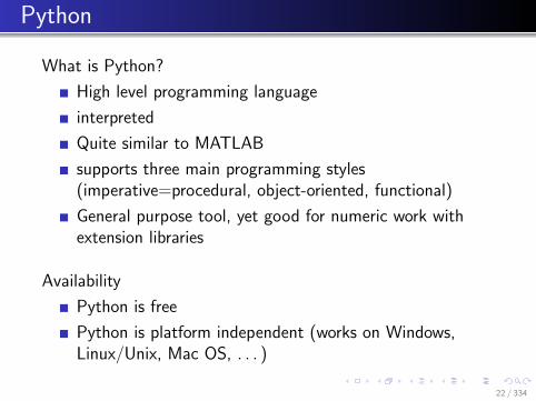
Python
What is Python?
High level programming language
interpreted
Quite similar to MATLAB
supports three main programming styles(imperative=procedural, object-oriented, functional)
General purpose tool, yet good for numeric work withextension libraries
Availability
Python is free
Python is platform independent (works on Windows,Linux/Unix, Mac OS, . . . )
22 / 334
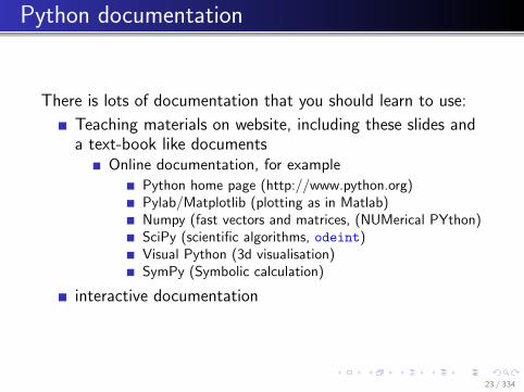
Python documentation
There is lots of documentation that you should learn to use:
Teaching materials on website, including these slides anda text-book like documents
Online documentation, for example
Python home page (http://www.python.org)Pylab/Matplotlib (plotting as in Matlab)Numpy (fast vectors and matrices, (NUMerical PYthon)SciPy (scientific algorithms, odeint)Visual Python (3d visualisation)SymPy (Symbolic calculation)
interactive documentation
23 / 334

Which Python version
There are currently two versions of Python:
Python 2.x andPython 3.x
We will use version 2.7 (compatible with numericalextension modules scipy, numpy, pylab).
Python 2.x and 3.x are incompatible although thechanges only affect very few commands.
See webpages for notes on installation of Python oncomputers.
24 / 334
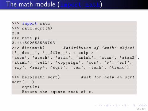
The math module (import math)
>>> import math
>>> math.sqrt (4)
2.0
>>> math.pi
3.141592653589793
>>> dir(math) #attributes of ’math’ object
[’__doc__ ’, ’__file__ ’, < snip >
’acos’, ’acosh’, ’asin’, ’asinh’, ’atan’, ’atan2’,
’atanh ’, ’ceil’, ’copysign ’, ’cos’, ’e’, ’erf’,
’exp’, <snip >, ’sqrt’, ’tan’, ’tanh’, ’trunc’]
>>> help(math.sqrt) #ask for help on sqrt
sqrt (...)
sqrt(x)
Return the square root of x.
25 / 334

Name spaces and modules
Three (good) options to access a module:
1 use the full name:
import math
print math.sin (0.5)
2 use some abbreviation
import math as m
print m.sin (0.5)
print m.pi
3 import all objects we need explicitly
from math import sin , pi
print sin (0.5)
print pi
26 / 334

Integer division (revisited) I
Reminder
>>> 1 / 2
0 # expected 0.5, not 0
Solutions:
change (at least) one of the integer numbers into afloating point number (i.e. 1 → 1.0).
>>> 1.0 / 2
0.5
Or use float function to convert variable to float
>>> a = 1
>>> b = 2
>>> 1 / float(b)
0.5
27 / 334
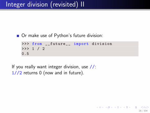
Integer division (revisited) II
Or make use of Python’s future division:
>>> from __future__ import division
>>> 1 / 2
0.5
If you really want integer division, use //:1//2 returns 0 (now and in future).
28 / 334

Coding style
29 / 334

Coding style
Python programs must follow Python syntax.
Python programs should follow Python style guide,because
readability is key (debugging, documentation, teameffort)conventions improve effectiveness
30 / 334

Common style guide: PEP8
See http://www.python.org/dev/peps/pep-0008/
This document gives coding conventions for the Python codecomprising the standard library in the main Python distribution.
This style guide evolves over time as additional conventions areidentified and past conventions are rendered obsolete by changes inthe language itself.
Many projects have their own coding style guidelines. In the eventof any conflicts, such project-specific guides take precedence forthat project.
One of Guido’s key insights is that code is read much more oftenthan it is written. The guidelines provided here are intended toimprove the readability of code and make it consistent across thewide spectrum of Python code. ”Readability counts”.
When not to follow this style guide:When applying the guideline would make the code less readable, even for someone who is used toreading code that follows this PEP.To be consistent with surrounding code that also breaks it (maybe for historic reasons) –although this is also an opportunity to clean up someone else’s mess (in true XP style).Because the code in question predates the introduction of the guideline and there is no otherreason to be modifying that code.
31 / 334

PEP8 Style guide
Indentation: use 4 spaces
One space around = operator: c = 5 and not c=5.
Spaces around arithmetic operators can vary: x = 3*a +
4*b is okay, but also okay to write x = 3 * a + 4 * b.
No space before and after parentheses: x = sin(x) butnot x = sin( x )
A space after comma: range(5, 10) and notrange(5,10).
No whitespace at end of line
No whitespace in empty line
One or no empty line between statements within function
Two empty lines between functions
One import statement per line
import first standand Python library, then third-partypackages (numpy, scipy, ...), then our own modules.
32 / 334
PEP8 Style Summary
Try to follow PEP8 guide, in particular for new code
Use tools to help us, for example Spyder editor can showPEP8 violations
pep8 program available to check source code.
33 / 334
Conditionals, if-else
34 / 334

Truth values I
The python values True and False are special inbuilt objects:
>>> a = True
>>> print(a)
True
>>> type(a)
<type ’bool’>
>>> b = False
>>> print(b)
False
>>> type(b)
<type ’bool’>
We can operate with these two logical values using booleanlogic, for example the logical and operation (and):
35 / 334
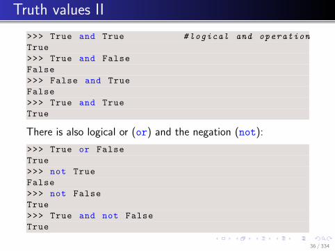
Truth values II
>>> True and True #logical and operation
True
>>> True and False
False
>>> False and True
False
>>> True and True
True
There is also logical or (or) and the negation (not):
>>> True or False
True
>>> not True
False
>>> not False
True
>>> True and not False
True
36 / 334

Truth values III
In computer code, we often need to evaluate some expressionthat is either true or false (sometimes called a “predicate”).For example:
>>> x = 30 # assign 30 to x
>>> x >= 30 # is x greater than or equal to 30?
True
>>> x > 15 # is x greater than 15
True
>>> x > 30
False
>>> x == 30 # is x the same as 30?
True
>>> not x == 42 # is x not the same as 42?
True
>>> x != 42 # is x not the same as 42?
True
37 / 334

if-then-else I
The if-else command allows to branch the execution pathdepending on a condition. For example:
>>> x = 30 # assign 30 to x
>>> if x > 30: # predicate: is x > 30
... print("Yes") # if True , do this
... else:
... print("No") # if False , do this
...
No
The general structure of the if-else statement is
if A:
B
else:
C
where A is the predicate.
38 / 334
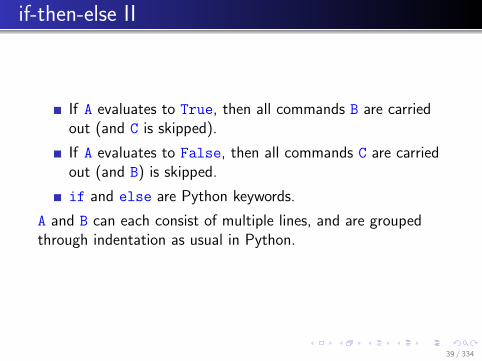
if-then-else II
If A evaluates to True, then all commands B are carriedout (and C is skipped).
If A evaluates to False, then all commands C are carriedout (and B) is skipped.
if and else are Python keywords.
A and B can each consist of multiple lines, and are groupedthrough indentation as usual in Python.
39 / 334

if-else example
def slength1(s):
""" Returns a string describing the
length of the sequence s"""
if len(s) > 10:
ans = ’very long’
else:
ans = ’normal ’
return ans
>>> slength1("Hello")
’normal ’
>>> slength1("HelloHello")
’normal ’
>>> slength1("Hello again")
’very long’
40 / 334
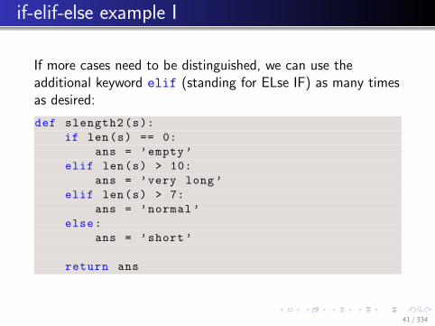
if-elif-else example I
If more cases need to be distinguished, we can use theadditional keyword elif (standing for ELse IF) as many timesas desired:
def slength2(s):
if len(s) == 0:
ans = ’empty’
elif len(s) > 10:
ans = ’very long’
elif len(s) > 7:
ans = ’normal ’
else:
ans = ’short’
return ans
41 / 334

if-elif-else example II>>> slength2("")
’empty ’
>>> slength2("Good Morning")
’very long’
>>> slength2("Greetings")
’normal ’
>>> slength2("Hi")
’short ’
LAB242 / 334
Sequences
43 / 334

Sequences overview
Different types of sequences
strings
lists (mutable)
tuples (immutable)
arrays (mutable, part of numpy)
They share common commands.
44 / 334

Strings
>>> a = "Hello World"
>>> type(a)
<type ’str’>
>>> len(a)
11
>>> print(a)
Hello World
Different possibilities to limit strings
’A string ’
"Another string"
"A string with a ’ in the middle"
"""A string with triple quotes can
extend over several
lines """
45 / 334

Strings 2 (exercise)
Enter this line on the Python prompt:>>> a="One"; b="Two"; c="Three"
Exercise: What do the following expressions evaluate to?
1 d = a + b + c
2 5 * d
3 d[0], d[1], d[2] (indexing)4 d[-1]
5 d[4:] (slicing)
46 / 334
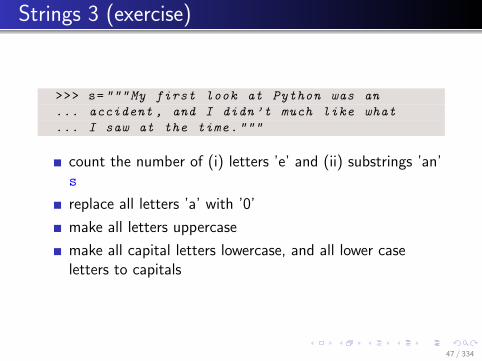
Strings 3 (exercise)
>>> s="""My first look at Python was an
... accident , and I didn’t much like what
... I saw at the time."""
count the number of (i) letters ’e’ and (ii) substrings ’an’s
replace all letters ’a’ with ’0’
make all letters uppercase
make all capital letters lowercase, and all lower caseletters to capitals
47 / 334

Lists
[] # the empty list
[42] # a 1-element list
[5, ’hello’, 17.3] # a 3-element list
[[1, 2], [3, 4], [5, 6]] # a list of lists
Lists store an ordered sequence of Python objects
Access through index (and slicing) as for strings.
Important function: range() (xrange)
use help(), often used list methods is append()
(In general computer science terminology, vector or array might be better name as the
actual implementation is not a linked list, but direct O(1) access through the index is
possible.)
48 / 334

Example program: using lists
>>> a = [] # creates a list
>>> a.append(’dog’) # appends string ’dog’
>>> a.append(’cat’) # ...
>>> a.append(’mouse’)
>>> print(a)
[’dog’, ’cat’, ’mouse’]
>>> print(a[0]) # access first element
dog # (with index 0)
>>> print(a[1]) # ...
cat
>>> print(a[2])
mouse
>>> print(a[-1]) # access last element
mouse
>>> print(a[-2]) # second last
cat
49 / 334
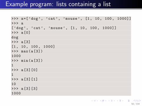
Example program: lists containing a list
>>> a=[’dog’, ’cat’, ’mouse’, [1, 10, 100, 1000]]
>>> a
[’dog’, ’cat’, ’mouse’, [1, 10, 100, 1000]]
>>> a[0]
dog
>>> a[3]
[1, 10, 100, 1000]
>>> max(a[3])
1000
>>> min(a[3])
1
>>> a[3][0]
1
>>> a[3][1]
10
>>> a[3][3]
1000
50 / 334
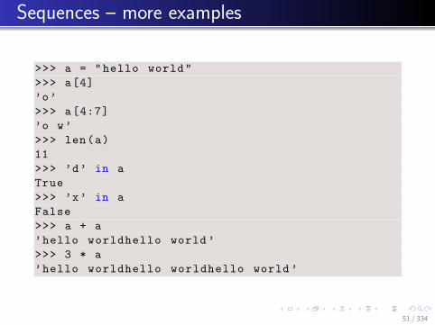
Sequences – more examples
>>> a = "hello world"
>>> a[4]
’o’
>>> a[4:7]
’o w’
>>> len(a)
11
>>> ’d’ in a
True
>>> ’x’ in a
False
>>> a + a
’hello worldhello world’
>>> 3 * a
’hello worldhello worldhello world’
51 / 334

Tuples I
tuples are very similar to lists
tuples are usually written using parentheses (↔ “roundbrackets”):
>>> t = (3, 4, 50)
>>> t
(3, 4, 50)
>>> type(t)
<type ’tuple’>
>>> l = [3, 4, 50] # compare with list object
>>> l
[3, 4, 50]
>>> type(l)
<type ’list’>
normal indexing and slicing (because tuple is a sequence)
52 / 334

Tuples II
>>> t[1]
4
>>> t[:-1]
(3, 4)
tuples are defined by the comma (!)
>>> a = 10, 20, 30
>>> type(a)
<type ’tuple’>
the parentheses are usually optional (but should bewritten anyway):
>>> a = (10, 20, 30)
>>> type(a)
<type ’tuple’>
53 / 334

Tuples III
So why do we need tuples (in addition to lists)?
1 use tuples if you want to make sure that a set of objectsdoesn’t change.
2 allow to assign several variables in one line (known astuple packing and unpacking)
x, y, z = 0, 0, 1
This allows ’instantaneous swap’ of values:
a, b = b, a
3 functions return tuples if they return more than one object
def f(x):
return x**2, x**3
a, b = f(x)
54 / 334
Tuples IV
4 tuples can be used as keys for dictionaries as they areimmutable
55 / 334

(Im)mutables
Strings — like tuples — are immutable:
>>> a = ’hello world’ # String example
>>> a[4] = ’x’
Traceback (most recent call last):
File "<stdin >", line 1, in ?
TypeError: object doesn ’t support
item assignment
strings can only be ’changed’ by creating a new string, forexample:
>>> a = a[0:3] + ’x’ + a[4:]
>>> a
’helxo world ’
56 / 334

Summary sequences
lists, strings and tuples (and arrays) are sequences. Forexample
list a = [1, 10, 42, 400] orstring a = ’hello world’
sequences share the following operations
a[i] returns i-th element of aa[i:j] returns elements i up to j − 1len(a) returns number of elements in sequencemin(a) returns smallest value in sequencemax(a) returns largest value in sequencex in a returns True if x is element in a
a + b concatenates a and b
n * a creates n copies of sequence a
In the table above, a and b are sequences, i, j and n areintegers.
57 / 334
Loops
58 / 334

Example programmes: for-loops I
animals = [’dog’, ’cat’, ’mouse’]
for animal in animals:
print("This is the {}".format(animal ))
produces this output:
This is the dog
This is the cat
This is the mouse
The range(n) command is used to create lists with increasinginteger values up to (but not including) n:
59 / 334

Example programmes: for-loops II
>>> range (6)
[0, 1, 2, 3, 4, 5]
>>> range (3)
[0, 1, 2]
for i in range (6):
print("the square of {} is {}"
.format(i, i ** 2))
produces this output:
the square of 0 is 0
the square of 1 is 1
the square of 2 is 4
the square of 3 is 9
the square of 4 is 16
the square of 5 is 25
60 / 334
Example programmes: for-loops III
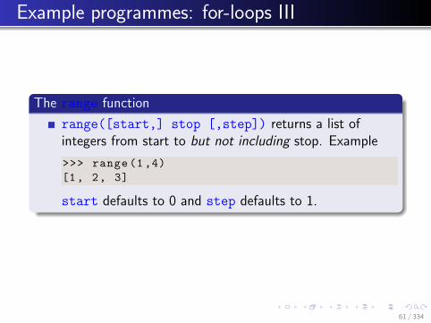
The range function
range([start,] stop [,step]) returns a list ofintegers from start to but not including stop. Example
>>> range (1,4)
[1, 2, 3]
start defaults to 0 and step defaults to 1.
61 / 334
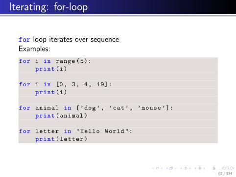
Iterating: for-loop
for loop iterates over sequenceExamples:
for i in range (5):
print(i)
for i in [0, 3, 4, 19]:
print(i)
for animal in [’dog’, ’cat’, ’mouse’]:
print(animal)
for letter in "Hello World":
print(letter)
62 / 334

Branching: If-then-else
Example 1 (if-then-else)
a = 42
if a > 0:
print("a is positive")
else:
print("a is negative or zero")
Example 2 (if-then-elif-else)
a = 42
if a > 0:
print("a is positive")
elif a == 0:
print("a is zero")
else:
print("a is negative")
63 / 334

Another iteration example
This example generates a sequence of numbers often used inhotels to label floors (more info)
def skip13(a, b):
result = []
for k in range (a,b):
if k == 13:
pass # do nothing
else:
result.append(k)
return result
64 / 334

Exercise range double
Write a function range double(n) that behaves in the sameway as the in-built python function range(n) but whichreturns twice the number for every entry. For example:
>>> range_double (4)
[0, 2, 4, 6]
>>> range_double (10)
[0, 2, 4, 6, 8, 10, 12, 14, 16, 18]
For comparison the behaviour of range:
>>> range (4)
[0, 1, 2, 3]
>>> range (10)
[0, 1, 2, 3, 4, 5, 6, 7, 8, 9]
LAB3
65 / 334

Exercise: First In First Out (FIFO) queue
Write a First-In-First-Out queue implementation, withfunctions:
add(name) to add a customer with name name (call thiswhen a new customer arrives)
next() to be called when the next customer will beserved. This function returns the name of the customer
show() to print all names of customers that are currentlywaiting
length() to return the number of currently waitingcustomers
66 / 334

Suggest to use a global variable q and define this in the firstline of the file by assigning an empty list: q = [].
67 / 334

While loops
a for loop iterates over a given sequence
a while loop iterates while a condition is fulfilled
Example:
x=64
while x>1:
x = x/2
print(x)
produces
32
16
8
4
2
1
68 / 334

While loop example 2
Determine ε:
eps = 1.0
while eps + 1 > 1:
eps = eps / 2.0
print("epsilon is {}".format(eps))
identical to
eps = 1.0
while True:
if eps + 1 == 1:
break # leaves innermost loop
eps = eps / 2.0
print("epsilon is {}".format(eps))
Output:
epsilon is 1.11022302463e-16
69 / 334
Some things revisited
70 / 334

What are variables?
In Python, variables are references to objects.This is why in the following example, a and b represent thesame list: a and b are two different references to the sameobject:
>>> a = [0, 2, 4, 6] # bind name ’a’ to list
>>> a # object [0,2,4,6].
[0, 2, 4, 6]
>>> b = a # bind name ’b’ to the same
>>> b # list object.
[0, 2, 4, 6]
>>> b[1] # show second element in list
2 # object.
>>> b[1] = 10 # modify 2nd elememnt (via b).
>>> b # show b.
[0, 100, 4, 6]
>>> a # show a.
[0, 100, 4, 6]
71 / 334

id, == and is
Two objects a and b are the same object if they live inthe same place in memory (id()). We check with id(a)
== id(b) or a is b.Two different objects can have the same value. We checkwith == See “Equality and identity“, section 3.5
>>> a = 1
>>> b = 1.0
>>> id(a); id(b)
4298187624 #not in the same place
4298197712 #in memory
>>> a is b #i.e. not the same objects
False
>>> a == b #but carry the same value
True
>>> a = [1, 2, 3]
>>> b = a #b is reference to object of a
>>> a is b #thus they are the same
True72 / 334
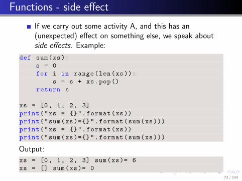
Functions - side effect
If we carry out some activity A, and this has an(unexpected) effect on something else, we speak aboutside effects. Example:
def sum(xs):
s = 0
for i in range(len(xs)):
s = s + xs.pop()
return s
xs = [0, 1, 2, 3]
print("xs = {}".format(xs))
print("sum(xs)={}".format(sum(xs)))
print("xs = {}".format(xs))
print("sum(xs)={}".format(sum(xs)))
Output:
xs = [0, 1, 2, 3] sum(xs)= 6
xs = [] sum(xs)= 0
73 / 334

Functions - side effect 2
Better ways to compute the sum of a list xs (or sequence ingeneral)
use in-built command sum(xs)
use indices to iterate over list
def sum(xs):
s=0
for i in range(len(xs)):
s = s + xs[i]
return s
or (better): iterate over list elements directly
def sum(xs):
s=0
for elem in xs
s = s + elem
return s
74 / 334

To print or to return?
A function that returns the control flow through thereturn keyword, will return the object given afterreturn.
A function that does not use the return keyword,returns the special object None.
Generally, functions should return a value
Generally, functions should not print anything
Calling functions from the prompt can cause someconfusion here: if the function returns a value and thevalue is not assigned, it will be printed.
75 / 334

Reading and writing data files
76 / 334

File input/output
It is a (surprisingly) common task to
read some input data file
do some calculation/filtering/processing with the data
write some output data file with results
77 / 334

Writing a text file I
>>> fout = open(’test.txt’, ’w’) # Write
>>> fout.write("first line\nsecond line")
>>> fout.close()
creates a file test.txt that reads
first line
second line
To write data, we need to use the ’w’ mode:
f = open(’mydatafile.txt’, ’w’)
If the file exists, it will be overridden with an empty filewhen the open command is executed.
The file object f has a method f.write which takes astring as in input argument.
Must close file at the end of writing process.
78 / 334

Reading a text file I
We create a file object f using
>>> f = open(’test.txt’, ’r’) # Read
and have different ways of reading the data:
Example 1 (readlines())f.readlines() returns a list of strings (each being oneline)
>>> f = open(’test.txt’, ’r’)
>>> lines = f.readlines ()
>>> f.close()
>>> lines
[’first line\n’, ’second line’]
79 / 334
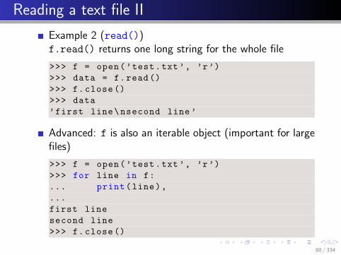
Reading a text file II
Example 2 (read())f.read() returns one long string for the whole file
>>> f = open(’test.txt’, ’r’)
>>> data = f.read()
>>> f.close()
>>> data
’first line\nsecond line’
Advanced: f is also an iterable object (important for largefiles)
>>> f = open(’test.txt’, ’r’)
>>> for line in f:
... print(line),
...
first line
second line
>>> f.close()
80 / 334

Reading a text file III
Advanced: Could use a context:
>>> with open(’test.txt’, ’r’) as f:
... data = f.read()
...
>>> data
’first line\nsecond line’
81 / 334

Reading a file, iterating over lines
Often we want to process line by line. Typical codefragment:
f = open(’myfile.txt’, ’r’)
lines = f.readlines ()
f.close()
# Then do some processing with the
# lines object
lines is a list of strings, each representing one line of thefile.
It is good practice to close a file as soon as possible.
82 / 334
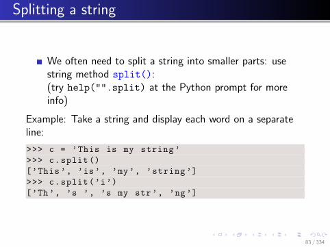
Splitting a string
We often need to split a string into smaller parts: usestring method split():(try help("".split) at the Python prompt for moreinfo)
Example: Take a string and display each word on a separateline:
>>> c = ’This is my string ’
>>> c.split()
[’This’, ’is’, ’my’, ’string ’]
>>> c.split(’i’)
[’Th’, ’s ’, ’s my str’, ’ng’]
83 / 334

Exercise: Shopping list
Given a list
bread 1 1.39
tomatoes 6 0.26
milk 3 1.45
coffee 3 2.99
Write program that computes total cost per item, and writesto shopping cost.txt:
bread 1.39
tomatoes 1.56
milk 4.35
coffee 8.97
84 / 334
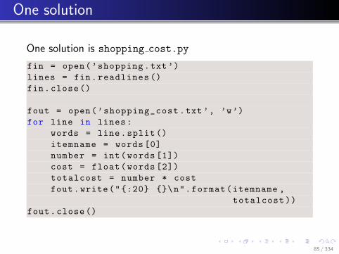
One solution
One solution is shopping cost.py
fin = open(’shopping.txt’)
lines = fin.readlines ()
fin.close()
fout = open(’shopping_cost.txt’, ’w’)
for line in lines:
words = line.split ()
itemname = words [0]
number = int(words [1])
cost = float(words [2])
totalcost = number * cost
fout.write("{:20} {}\n".format(itemname ,
totalcost ))
fout.close()
85 / 334

Exercise
Write function print line sum of file(filename) thatreads a file of name filename containing numbers separatedby spaces, and which computes and prints the sum for eachline. A data file might look like
1 2 4 67 -34 340
0 45 3 2
17
LAB4
86 / 334

Exceptions
87 / 334

Exceptions
Errors arising during the execution of a program result in“exceptions”.We have seen exceptions before, for example when dividingby zero:
>>> 4.5 / 0
Traceback (most recent call last):
File "<stdin >", line 1, in ?
ZeroDivisionError: float division
or when we try to access an undefined variable:
>>> print(x)
Traceback (most recent call last):
File "<stdin >", line 1, in ?
NameError: name ’x’ is not defined
Exceptions are a modern way of dealing with error situationsWe will now see how
what exceptions are coming with Pythonwe can “catch” exceptionswe can raise (“throw”) exceptions in our code
88 / 334

In-built Python exceptions I
Python’s inbuilt exceptions can be found in the exceptions
module.Users can provide their own exception classes (by inheriting from Exception).
>>> import exceptions
>>> help(exceptions)
BaseException
Exception
StandardError
ArithmeticError
FloatingPointError
OverflowError
ZeroDivisionError
AssertionError
AttributeError
BufferError
EOFError
EnvironmentError
IOError
OSError
ImportError
LookupError
IndexError
KeyError
MemoryError
NameError
UnboundLocalError
ReferenceError
89 / 334

In-built Python exceptions II
RuntimeError
NotImplementedError
SyntaxError
IndentationError
TabError
SystemError
TypeError
ValueError
UnicodeError
UnicodeDecodeError
UnicodeEncodeError
UnicodeTranslateError
StopIteration
Warning
BytesWarning
DeprecationWarning
FutureWarning
ImportWarning
PendingDeprecationWarning
RuntimeWarning
SyntaxWarning
UnicodeWarning
UserWarning
GeneratorExit
KeyboardInterrupt
SystemExit
90 / 334

Catching exceptions (1)
suppose we try to read data from a file:
f = open(’myfilename.dat’, ’r’)
for line in f.readlines ():
print(line)
If the file doesn’t exist, then the open() function raises anInput-Output Error (IOError):IOError: [Errno 2] No such file or directory: ’myfilename.dat’
We can modify our code to catch this error:
1 try:
2 f = open(’myfilename.dat’, ’r’)
3 except IOError:
4 print("The file couldn ’t be opened."),
5 print("This program stops here.")
6 import sys
7 sys.exit (1) #a way to exit the program
89 for line in f.readlines ():
10 print(line)
which produces this message:
The file couldn ’t be opened. This program stops here.
91 / 334

Catching exceptions (2)
The try branch (line 2) will be executed.
Should an IOError exception be raised the the exceptbranch (starting line 4) will be executed.
Should no exception be raised in the try branch, then theexcept branch is ignored, and the program carries onstarting in line 9.
Catching exceptions allows us to take action on errorsthat occur
For the file-reading example, we could ask the user toprovide another file name if the file can’t be opened.
Catching an exception once an error has occurred may beeasier than checking beforehand whether a problem willoccur (“It is easier to ask forgiveness than getpermission”.)
92 / 334
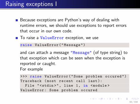
Raising exceptions I
Because exceptions are Python’s way of dealing withruntime errors, we should use exceptions to report errorsthat occur in our own code.
To raise a ValueError exception, we use
raise ValueError("Message")
and can attach a message "Message" (of type string) tothat exception which can be seen when the exception isreported or caught.For example
>>> raise ValueError("Some problem occured")
Traceback (most recent call last):
File "<stdin >", line 1, in <module >
ValueError: Some problem occured
93 / 334

Raising exceptions II
Often used is the NotImplementedError in incrementalcoding:
def my_complicated_function(x):
message = "Function called with x={}".format(x))
raise NotImplementedError(msg)
If we call the function:
>>> my_complicated_function (42)
Traceback (most recent call last):
File "<stdin >", line 1, in <module >
File "<stdin >", line 2, in my_complicated_function
NotImplementedError: Function called with x=42
94 / 334
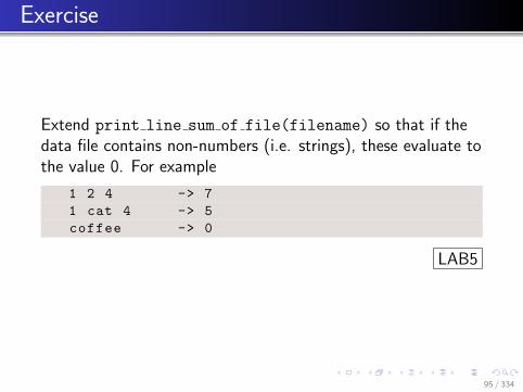
Exercise
Extend print line sum of file(filename) so that if thedata file contains non-numbers (i.e. strings), these evaluate tothe value 0. For example
1 2 4 -> 7
1 cat 4 -> 5
coffee -> 0
LAB5
95 / 334

Printing
96 / 334

Printing: print without parentheses I
Option 1: list the variables to be printed, separated bycomma, no parentheses. Convenient, but not flexible.
This way of using print will not work with python 3.x
>>> a = 10
>>> print a
10
>>> print "The number is", a
The number is 10
>>> s = "hello"
>>> print "The number is", a, "and s is", s
The number is 10 and s is hello
>>> print a, s # the comma adds a space
10 "hello"
97 / 334

Printing: print with parentheses I
Option 2: construct some string s, then print this stringusing the print function
Works with Python 2.7 and future python versions
>>> s = "I am the string to be printed"
>>> print(s)
I am the string to be printed
The question is, how can we construct the string s? Wetalk about string formatting.
98 / 334

String formatting: the percentage (%) operator I
% operator syntax
Syntax: A % B
where A is a string, and B a Python object, or a tuple ofPython objects.The format string A needs to contain k format specifiers if thetuple has length k. The operation returns a string.
Example: basic formatting of one number
>>> import math
>>> p = math.pi
>>> "%f" % p # format p as float (%f)
’3.141593 ’ # returns string
>>> "%d" % p # format p as integer (%d)
’3’
>>> "%e" % p # format p in exponential style
99 / 334

String formatting: the percentage (%) operator II
’3.141593e+00’
>>> "%g" % p # format using fewer characters
’3.14159 ’
The format specifiers can be combined with arbitrarycharacters in string:
>>> ’the value of pi is approx %f’ % p
’the value of pi is approx 3.141593 ’
>>> ’%d is my preferred number ’ % 42
’42 is my preferred number ’
Printing multiple objects
>>> "%d times %d is %d" % (10, 42, 10 * 42)
’10 times 42 is 420’
>>> "pi=%f and 3*pi=%f is approx 10" % (p, 3*p)
’pi =3.141593 and 3*pi =9.424778 is approx 10’
100 / 334

Fixing width and/or precision of resulting string I
>>> ’%f’ % 3.14 # default width and precision
’3.140000 ’
>>> ’%10f’ % 3.14 # 10 characters long
’ 3.140000 ’
>>> ’%10.2f’ % 3.14 # 10 long , 2 post -dec digits
’ 3.14’
>>> ’%.2f’ % 3.14 # 2 post -dec digits
’3.14’
>>> ’%.14f’ % 3.14 # 14 post -decimal digits
’3.14000000000000 ’
Can also use format specifier %s to format strings (typicallyused to align columns in tables, or such).
101 / 334

Common formatting specifiers
A list of common formatting specifiers, with example outputfor the astronomical unit (AU) which is the distance fromEarth to Sun [in metres]:
>>> AU = 149597870700 # astronomical unit [m]
>>> "%f" % AU # line 1 in table
’149597870700.000000 ’
specifier style Example output for AU
%f floating point 149597870700.000000
%e exponential notation 1.495979e+11
%g shorter of %e or %f 1.49598e+11
%d integer 149597870700
%s str() 149597870700
%r repr() 149597870700L
102 / 334
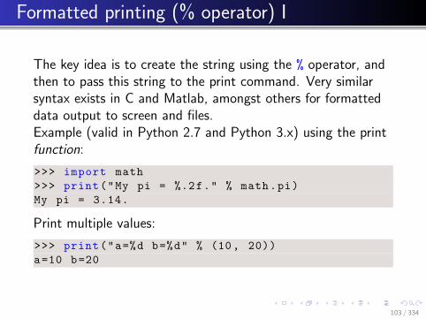
Formatted printing (% operator) I
The key idea is to create the string using the % operator, andthen to pass this string to the print command. Very similarsyntax exists in C and Matlab, amongst others for formatteddata output to screen and files.Example (valid in Python 2.7 and Python 3.x) using the printfunction:
>>> import math
>>> print("My pi = %.2f." % math.pi)
My pi = 3.14.
Print multiple values:
>>> print("a=%d b=%d" % (10, 20))
a=10 b=20
103 / 334

New style string formatting (format method) I
A new system of built-in formatting has been proposed and ismeant to replace the old-style percentage operator formatting(%) in the long term.Basic ideas in examples:
Pairs of curly braces are the placeholders.
>>> "{} needs {} pints".format(’Peter’, 4)
’Peter needs 4 pints’
Can index into the list of objects:
>>> "{0} needs {1} pints".format(’Peter’ ,4)
’Peter needs 4 pints’
>>> "{1} needs {0} pints".format(’Peter’ ,4)
’4 needs Peter pints’
We can refer to objects through a name:
104 / 334

New style string formatting (format method) II
>>> "{name} needs {number} pints".format (\
... name=’Peter’,number =4)
’Peter needs 4 pints’
Formatting behaviour of %f can be achieved through{:f}, (same for %d, %e, etc)
>>> "Pi is approx {:f}.".format(math.pi)
’Pi is approx 3.141593. ’
Width and post decimal digits can be specified as before:
>>> "Pi is approx {:6.2f}.".format(math.pi)
’Pi is approx 3.14.’
>>> "Pi is approx {:.2f}.".format(math.pi)
’Pi is approx 3.14.’
105 / 334

New style string formatting (format method) III
This is a powerful and elegant way of string formatting.
Further Reading
Exampleshttp://docs.python.org/library/string.html#format-examples
Python Enhancement Proposal 3101
106 / 334

What formatting should I use? I
The .format method most elegant and versatile
% operator style okay, links to Matlab, C, ...
Choice partly a matter of taste
Should be aware (in a passive sense) of different possiblestyles (so we can read code from others)
try to use print with parenthesis (i.e. compatible withPython 3.x) for code you write
107 / 334
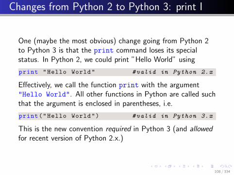
Changes from Python 2 to Python 3: print I
One (maybe the most obvious) change going from Python 2to Python 3 is that the print command loses its specialstatus. In Python 2, we could print ”Hello World” using
print "Hello World" #valid in Python 2.x
Effectively, we call the function print with the argument"Hello World". All other functions in Python are called suchthat the argument is enclosed in parentheses, i.e.
print("Hello World") #valid in Python 3.x
This is the new convention required in Python 3 (and allowedfor recent version of Python 2.x.)
108 / 334

Advanced: “str“ and “repr“: “str“ I
All objects in Python should provide a method str whichreturns a nice string representation of the object. This methoda. str () is called when we apply the str function toobject a:
>>> a = 3.14
>>> a.__str__ ()
’3.14’
>>> str(a)
’3.14’
The str function is extremely convenient as it allows us toprint more complicated objects, such as
>>> b = [3, 4.2, [’apple’, ’banana ’], (0, 1)]
>>> str(b)
"[3, 4.2, [’apple ’, ’banana ’], (0, 1)]"
109 / 334

Advanced: “str“ and “repr“: “str“ II
The string method x. str of object x is called implicitly,when we
use the ”%s” format specifier in %-operator formatting toprint x
use the ”{}” format specifier in .format to print x
pass the object x directly to the print command
>>> print(b)
[3, 4.2, [’apple’, ’banana ’], (0, 1)]
>>> "%s" % b
[3, 4.2, [’apple’, ’banana ’], (0, 1)]
>>> "{}".format(b)
[3, 4.2, [’apple’, ’banana ’], (0, 1)]
110 / 334

Advanced: “str“ and “repr“: “repr“ I
The repr function, should convert a given object into anas accurate as possible string representation
so that (ideally) this string can be used to re-create theobject using the eval function.
The repr function will generally provide a more detailedstring than str.
Applying repr to the object x will attempt to callx. repr ().
111 / 334
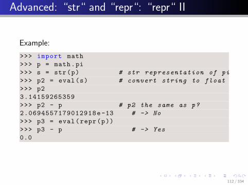
Advanced: “str“ and “repr“: “repr“ II
Example:
>>> import math
>>> p = math.pi
>>> s = str(p) # str representation of pi
>>> p2 = eval(s) # convert string to float
>>> p2
3.14159265359
>>> p2 - p # p2 the same as p?
2.0694557179012918e-13 # -> No
>>> p3 = eval(repr(p))
>>> p3 - p # -> Yes
0.0
112 / 334

Advanced: “str“ and “repr“: “repr“ III
We can convert an object to its str() or repr() presentationusing the format specifiers %s and %r, respectively.
>>> import math
>>> "%s" % math.pi
’3.14159265359 ’
>>> "%r" % math.pi
’3.141592653589793 ’
113 / 334

Higher Order Functions
114 / 334

Motivational exercise: function tables
Write a function print x2 table() that prints a table ofvalues of f(x) = x2 for x = 0, 0.5, 1.0, ..2.5, i.e.
0.0 0.0
0.5 0.25
1.0 1.0
1.5 2.25
2.0 4.0
2.5 6.25
Then do the same for f(x) = x3
Then do the same for f(x) = sin(x)
115 / 334
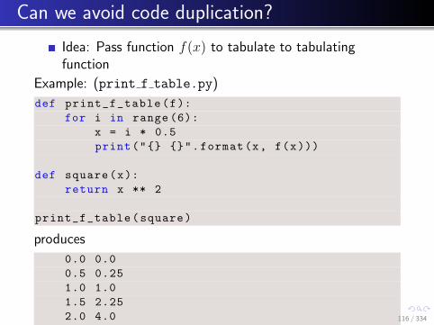
Can we avoid code duplication?
Idea: Pass function f(x) to tabulate to tabulatingfunction
Example: (print f table.py)
def print_f_table(f):
for i in range (6):
x = i * 0.5
print("{} {}".format(x, f(x)))
def square(x):
return x ** 2
print_f_table(square)
produces
0.0 0.0
0.5 0.25
1.0 1.0
1.5 2.25
2.0 4.0
2.5 6.25116 / 334
Can we avoid code duplication (2)?
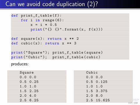
def print_f_table(f):
for i in range (6):
x = i * 0.5
print("{} {}".format(x, f(x)))
def square(x): return x ** 2
def cubic(x): return x ** 3
print("Square"); print_f_table(square)
print("Cubic"); print_f_table(cubic)
produces:
Square
0.0 0.0
0.5 0.25
1.0 1.0
1.5 2.25
2.0 4.0
2.5 6.25
Cubic
0.0 0.0
0.5 0.125
1.0 1.0
1.5 3.375
2.0 8.0
2.5 15.625117 / 334

Functions are first class objects
Functions are first class objects ↔ functions can be givento other functions as arguments
Example (trigtable.py):
import math
funcs = (math.sin , math.cos)
for f in funcs:
for x in [0, math.pi / 2]:
print("{}({:.3f}) = {:.3f}".format(
f.__name__ , x, f(x)))
sin (0.000) = 0.000
sin (1.571) = 1.000
cos (0.000) = 1.000
cos (1.571) = 0.000
118 / 334

Module files
119 / 334
Writing module files
Motivation: it is useful to bundle functions that are usedrepeatedly and belong to the same subject area into onemodule file (also called “library”)
Every Python file can be imported as a module.
If this module file has a main program, then this isexecuted when the file is imported. This can be desiredbut sometimes it is not.
We describe how a main program can be written which isonly executed if the file is run on its own but not if isimported as a library.
120 / 334

The internal name variable (1)
Here is an example of a module file saved as module1.py:
def someusefulfunction ():
pass
print("My name is {}".format(__name__ ))
We can execute this module file, and the output is
My name is __main__
The internal variable name takes the (string) value" main " if the program file module1.py is executed.
On the other hand, we can import module1.py in anotherfile, for example like this:
import module1
The output is now:
My name is module1
This means that name inside a module takes the value ofthe module name if the file is imported.
121 / 334

The internal name variable (2)
In summary
name is " main " if the module file is run on itsownname is the name (type string) of the module if the
module file is imported.
We can therefore use the following if statement inmodule1.py to write code that is only run when the moduleis executed on its own:
def someusefulfunction ():
pass
if __name__ == "__main__":
print("I am running on my own.")
This is useful to keep test programs or demonstrations of theabilities of a library module in this “conditional” mainprogram. 122 / 334

Default and Keyword functionarguments
123 / 334

Default argument values (1)
Motivation:
suppose we need to compute the area of rectangles andwe know the side lengths a and b.Most of the time, b=1 but sometimes b can take othervalues.
Solution 1:
def area(a, b):
return a * b
print("the area is {}".format(area(3, 1)))
print("the area is {}".format(area (2.5, 1)))
print("the area is {}".format(area (2.5, 2)))
Working perfectly.
124 / 334
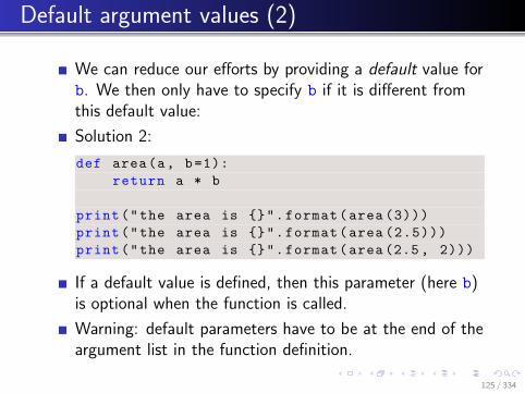
Default argument values (2)
We can reduce our efforts by providing a default value forb. We then only have to specify b if it is different fromthis default value:
Solution 2:
def area(a, b=1):
return a * b
print("the area is {}".format(area (3)))
print("the area is {}".format(area (2.5)))
print("the area is {}".format(area (2.5, 2)))
If a default value is defined, then this parameter (here b)is optional when the function is called.
Warning: default parameters have to be at the end of theargument list in the function definition.
125 / 334

Keyword argument values (1)
We can call functions with a “keyword” and a value.(The keyword is the name of the variable in the function.)Here is an example
def f(a, b, c):
print("a = {}, b = {}, c = {}"
.format(a, b, c))
f(1, 2, 3)
f(c=3, a=1, b=2)
f(1, c=3, b=2)
which produces this output:
a = 1, b = 2, c = 3
a = 1, b = 2, c = 3
a = 1, b = 2, c = 3
If we use only keyword arguments in the function call,then we don’t need to know the order of the arguments.(This is good.) 126 / 334

Keyword argument values (2)
Can combine default value arguments and keywordarguments
Example: we use 100 subdivisions unless the user providesa number
def trapez(function , a, b, subdivisions =100):
#code missing here
import math
int1 = trapez(a=0, b=10, function=math.sin)
int2 = trapez(b=0, function=math.exp , \
subdivisions =1000, a=-0.5)
Note that choosing meaningful variable names in thefunction definition makes the function more user friendly.
127 / 334
Keyword argument values (3)
You may have met default arguments and keyword argumentsbefore, for example
the string method split uses white space as the defaultvalue for splitting
the open function uses r (for Reading) as a default value
LAB6
128 / 334
Global and local variables,Name spaces
129 / 334
Name spaces — what can be seen where? (1)
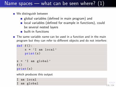
We distinguish between
global variables (defined in main program) andlocal variables (defined for example in functions), couldbe several nested layersbuilt-in functions
The same variable name can be used in a function and in the mainprogram but they can refer to different objects and do not interfere:
def f():
x = ’I am local ’
print(x)
x = ’I am global ’
f()
print(x)
which produces this output
I am local
I am global
Imported modules have their own name space.
130 / 334

Name spaces (2)
. . . so global and local variables can’t see each other?
not quite. Let’s read the small print:If — within a function – we try to access a variable,then Python will look for this variable
first in the local name space (i.e. within that function)then in the global name space (!)
If the variable can’t be found, a NameError is raised.
This means, we can read global variables from functions.Example:
def f():
print(x)
x = ’I am global ’
f()
Output:
I am global
131 / 334

Name spaces (3)
but local variables “shadow” global variables:
def f():
y = ’I am local y’
print(x)
print(y)
x = ’I am global x’
y = ’I am global y’
f()
print("back in main:")
print(y)
Output:
I am global x
I am local y
back in main:
I am global y
To modify global variables within a local namespace, weneed to use the global keyword.(This is not recommended so we won’t explain it. See also next slide.)
132 / 334

Why should I care about global variables?
Generally, the use of global variables is not recommended:
functions should take all necessary input as argumentsandreturn all relevant output.This makes the functions work as independent moduleswhich is good engineering practice.
However, sometimes the same constant or variable (suchas the mass of an object) is required throughout aprogram:
it is not good practice to define this variable more thanonce (it is likely that we assign different values and getinconsistent results)in this case — in small programs — the use of(read-only) global variables may be acceptable.Object Oriented Programming provides a somewhatneater solution to this.
133 / 334

Python’s look up rule
When coming across an identifier, Python looks for this inthe following order in
the local name space (L)(if appropriate in the next higher level local namespace), (L2, L3, . . . )the global name space (G)the set of built-in commands (B)
This is summarised as “LGB” or “LnGB”.
If the identifier cannot be found, a NameError is raised.
134 / 334

Python shells and IDE
135 / 334

Integrated Development Environment: combine
editor and prompt: IDLE
IDLE http://en.wikipedia.org/wiki/IDLE (Python)(comes with Python)
two windows: program and python prompt
F5 to execute Python program
Simple, (written in Python → portable)
136 / 334

IPython (interactive python)
Interactive Python (ipython from DOS/Unix-shell)
command history (across sessions), auto completion,
special commands:
%run test will execute file test.py in current namespace (in contrast to IDLE this does not remove allexisting objects from global name space)%reset can delete all objects if required%edit will open an editoruse range? instead of help(range)%logstart will log your session%prun will profile code%timeit can measure execution time%load loads file for editing
Much (!) more (read at http://ipython.scipy.org)
137 / 334

IPython’s QT console
Prompt as IPython (with all it’s features): running in agraphics console rather than in text console
but allows multi-line editing of command history
provides on-the-fly syntax highlighting
can inline matplotlib figures
Read more at http://ipython.org/ipython-doc/dev/interactive/qtconsole.html
138 / 334

... and many others
Including
IPython notebook (http://ipython.org/ipython-doc/dev/interactive/htmlnotebook.html). See videodemo at http://youtu.be/HaS4NXxL5Qc
Eclipse
vi, vim
Kate
Sublime Text
Spyder
139 / 334

List comprehension
140 / 334

List comprehension I
List comprehension follows the mathematical “set buildernotation”
Convenient way to process a list into another list (withoutfor-loop).
Examples
>>> [2 ** i for i in range (10)]
[1, 2, 4, 8, 16, 32, 64, 128, 256, 512, 1024]
>>> [x ** 2 for x in range (10)]
[0, 1, 4, 9, 16, 25, 36, 49, 64, 81]
>>> [x for x in range (10) if x > 5]
[6, 7, 8, 9]
Can be useful to populate lists with numbers quickly
141 / 334

List comprehension II
Example 1:
>>> xs = [i for i in range (10)]
>>> xs
[0, 1, 2, 3, 4, 5, 6, 7, 8, 9]
>>> ys = [x ** 2 for x in xs]
>>> ys
[0, 1, 4, 9, 16, 25, 36, 49, 64, 81]
Example 2:
>>> import math
>>> xs = [0.1 * i for i in range (5)]
>>> ys = [math.exp(x) for x in xs]
>>> xs
[0.0, 0.1, 0.2, 0.3, 0.4]
>>> ys
[1.0, 1.1051709180756477 , 1.2214027581601699 ,
1.3498588075760032 , 1.4918246976412703]
142 / 334

List comprehension III
Example 3
>>> words = ’The quick brown fox jumps \
... over the lazy dog’.split()
>>> print words
[’The’, ’quick ’, ’brown ’, ’fox’, ’jumps ’,
’over’, ’the’, ’lazy’, ’dog’]
>>> stuff = [[w.upper(), w.lower(), len(w)]
for w in words]
>>> for i in stuff:
... print(i)
...
[’THE’, ’the’, 3]
[’QUICK ’, ’quick ’, 5]
[’BROWN ’, ’brown ’, 5]
[’FOX’, ’fox’, 3]
[’JUMPS ’, ’jumps ’, 5
[’OVER’, ’over’, 4]
143 / 334

List comprehension IV
[’THE’, ’the’, 3]
[’LAZY’, ’lazy’, 4]
[’DOG’, ’dog’, 3]
144 / 334

List comprehension with conditional
Can extend list comprehension syntax with if
CONDITION to include only elements for whichCONDITION is true.
Example:
>>> [i for i in range (10)]
[0, 1, 2, 3, 4, 5, 6, 7, 8, 9]
>>> [i for i in range (10) if i > 5]
[6, 7, 8, 9]
>>> [i for i in range (10) if i ** 2 > 5]
[3, 4, 5, 6, 7, 8, 9]
145 / 334

Dictionaries
146 / 334

Dictionaries I
Python provides another data type: the dictionary.Dictionaries are also called “associative arrays” and “hash tables”.
Dictionaries are unordered sets of key-value pairs.
An empty dictionary can be created using curly braces:
>>> d = {}
Keyword-value pairs can be added like this:
>>> d[’today’] = ’22 deg C’ #’today ’ is key
# ’22 deg C’ is value
>>> d[’yesterday ’] = ’19 deg C’
d.keys() returns a list of all keys:
>>> d.keys()
[’yesterday ’, ’today ’]
147 / 334

Dictionaries IIWe can retrieve values by using the keyword as the index:
>>> print d[’today’]
22 deg C
148 / 334

Dictionaries IIIHere is a more complex example:
order = {} # create empty dictionary
#add orders as they come in
order[’Peter ’] = ’Pint of bitter ’
order[’Paul’] = ’Half pint of Hoegarden ’
order[’Mary’] = ’Gin Tonic ’
#deliver order at bar
for person in order.keys ():
print("{} requests {}".format(person , order[person ]))
which produces this output:
Paul requests Half pint of Hoegarden
Peter requests Pint of bitter
Mary requests Gin Tonic
149 / 334

Dictionaries IVSome more technicalities:
The keyword can be any (immutable) Python object.This includes:
numbersstringstuples.
dictionaries are very fast in retrieving values (when giventhe key)
150 / 334

Dictionaries V
What are dictionnaries good for? Consider this example:
dic = {}
dic["Hans"] = "room 1033"
dic["Andy C"] = "room 1031"
dic["Ken"] = "room 1027"
for key in dic.keys ():
print("{} works in {}"
.format(key , dic[key]))
Output:
Hans works in room 1033
Andy C works in room 1031
Ken works in room 1027
Without dictionary:
151 / 334

Dictionaries VI
people = ["Hans", "Andy C", "Ken"]
rooms = ["room 1033", "room 1031", \
"room 1027"]
# possible inconsistency here since we have
# two lists
if not len(people) == len(rooms):
raise ValueError("people and rooms " +
"differ in length")
for i in range(len(rooms )):
print ("{} works in {}".format(people[i],
rooms[i])
152 / 334

Iterating over dictionaries
Iterate over the dictionary itself is equivalent to iterating overthe keys. Example:
order = {} # create empty dictionary
order[’Peter ’] = ’Pint of bitter ’
order[’Paul’] = ’Half pint of Hoegarden ’
order[’Mary’] = ’Gin Tonic ’
#iterating over keys:
for person in order.keys ():
print person , "requests", order[person]
#is equivalent to iterating over the dictionary:
for person in order:
print person , "requests", order[person]
153 / 334

Summary dictionaries
What to remember:
Python provides dictionaries
very powerful construct
a bit like a data base (and values can be dictionaryobjects)
fast to retrieve value
likely to be useful if you are dealing with two lists at thesame time (possibly one of them contains the keywordand the other the value)
useful if you have a data set that needs to be indexed bystrings or tuples (or other immutable objects)
154 / 334

Recursion
155 / 334

Recursion
Recursion in a screen recording program, where the smallerwindow contains a snapshot of the entire screen. Source:
http://en.wikipedia.org/wiki/Recursion
156 / 334

Recursion example: factorial
Computing the factorial (i.e. n!) can be done bycomputing (n− 1)!n“, i.e. we reduce the problem of sizen to a problem of size n− 1.
For recursive problems, we always need a base case. Forthe factorial we know that “0! = 1“
For n=4:
4! = 3! · 4 (1)
= 2! · 3 · 4 (2)
= 1! · 2 · 3 · 4 (3)
= 0! · 1 · 2 · 3 · 4 (4)
= 1 · 1 · 2 · 3 · 4 (5)
= 24. (6)
157 / 334

Recursion example
Python code to compute the factorial recursively::
def factorial(n):
if n == 0:
return 1
else:
return n * factorial(n-1)
Usage output:
>>> factorial (0)
factorial (0)
1
>>> factorial (2)
2
>>> factorial (4)
24
158 / 334
Recursion example Fibonacci numbers
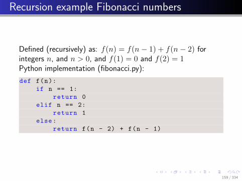
Defined (recursively) as: f(n) = f(n− 1) + f(n− 2) forintegers n, and n > 0, and f(1) = 0 and f(2) = 1Python implementation (fibonacci.py):
def f(n):
if n == 1:
return 0
elif n == 2:
return 1
else:
return f(n - 2) + f(n - 1)
159 / 334

Recursion exercises
Write a function recsum(n) that sums the numbers from1 to n recursively
Study the recursive Fibonacci function:
what is the largest number n for which we canreasonable compute f(n) within a minutes?Can you write faster versions of Fibonacci? (There arefaster versions with and without recursion.)
160 / 334
Common Computational Tasks
161 / 334

Common Computational Tasks
Data file processing, python & numpy (array processing)
Random number generation and fourier transforms(numpy)
Linear algebra (numpy)
Interpolation of data (scipy.interpolation.interp)
Fitting a curve to data (scipy.optimize.curve fit)
Integrating a function numerically(scipy.integrate.quad)
Integrating a ordinary differential equation numerically(scipy.integrate.odeint)
Finding the root of a function(scipy.optimize.fsolve,scipy.optimize.brentq)
Minimising a function (scipy.optimize.fmin)
Symbolic manipulation of terms, including integration anddifferentiation (sympy)
162 / 334

Root finding
163 / 334
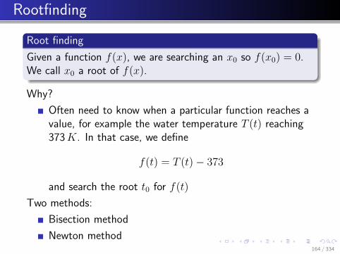
Rootfinding
Root finding
Given a function f(x), we are searching an x0 so f(x0) = 0.We call x0 a root of f(x).
Why?
Often need to know when a particular function reaches avalue, for example the water temperature T (t) reaching373K. In that case, we define
f(t) = T (t)− 373
and search the root t0 for f(t)
Two methods:
Bisection method
Newton method164 / 334

The bisection algorithm
Function: bisect(f, a, b)
Assumptions:Given: a (float)Given: b (float)Given: f(x), continuous with single root in [a, b], i.e.f(a)f(b) < 0Given: ftol (float), for example ftol=1e-6
The bisection method returns x so that |f(x)| <ftol
1 x = (a+ b)/2
2 while |f(x)| > ftol doif f(x)f(a) > 0then a← x #throw away left halfelse b← x #throw away right halfx = (a + b)/2
3 return x165 / 334
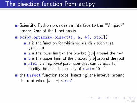
The bisection function from scipy
Scientific Python provides an interface to the “Minpack”library. One of the functions is
scipy.optimize.bisect(f, a, b[, xtol])
f is the function for which we search x such thatf(x) = 0a is the lower limit of the bracket [a,b] around the rootb is the upper limit of the bracket [a,b] around the rootxtol is an optional parameter that can be used tomodify the default accuracy of xtol= 10−12
the bisect function stops ’bisecting’ the interval aroundthe root when |b− a| <xtol.
166 / 334
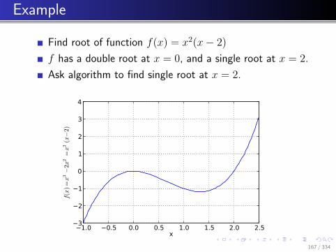
Example
Find root of function f(x) = x2(x− 2)
f has a double root at x = 0, and a single root at x = 2.
Ask algorithm to find single root at x = 2.
1.0 0.5 0.0 0.5 1.0 1.5 2.0 2.5x
3
2
1
0
1
2
3
4
f(x)=x
3−
2x2
=x
2(x−
2)
167 / 334

Using bisection algorithm from scipy
from scipy.optimize import bisect
def f(x):
""" returns f(x)=x^3-2x^2. Has roots at
x=0 (double root) and x=2"""
return x ** 3 - 2 * x ** 2
#main program starts here
x = bisect(f, a=1.5, b=3, xtol=1e-6)
print("Root x is approx. x={:14.12g}.".format(x))
print("The error is less than 1e-6.")
print("The exact error is {}.".format (2 - x))
generates this:
Root x is approx. x= 2.00000023842.
The error is less than 1e-6.
The exact error is -2.38418579102e-07.
168 / 334

The Newton method
Newton method for root finding: look for x0 so thatf(x0) = 0.
Idea: close to the root, the tangent of f(x) is likely topoint to the root. Make use of this information.
Algorithm:while |f(x)| >ftol, do
x = x− f(x)
f ′(x)
where f ′(x) = dfdx(x).
Much better convergence than bisection method
but not guaranteed to converge.
Need a good initial guess x for the root.
169 / 334

Using Newton algorithm from scipy
from scipy.optimize import newton
def f(x):
""" returns f(x)=x^3-2x^2. Has roots at
x=0 (double root) and x=2"""
return x ** 3 - 2 * x ** 2
#main program starts here
x = newton(f, x0 =1.6)
print("Root x is approx. x={:14.12g}.".format(x))
print("The error is less than 1e-6.")
print("The exact error is {}.".format (2 - x))
generates this:
Root x is approx. x= 2.
The error is less than 1e-6.
The exact error is 9.7699626167e-15.
170 / 334

Comparison Bisection & Newton method
Bisection method
Requires root in bracket[a, b]
guaranteed to converge(for single roots)
Library function:scipy.optimize.bisect
Newton method
Requires good initial guessx for root x0
may never converge
but if it does, it is quickerthan the bisection method
Library function:scipy.optimize.Newton
171 / 334

Root finding summary
Given the function f(x), applications for root findinginclude:
to find x1 so that f(x1) = y for a given y (this isequivalent to computing the inverse of the function f).to find crossing point xc of two functions f1(x) andf2(x) (by finding root of difference functiong(x) = f1(x)− f2(x))
Recommended method: scipy.optimize.brentq whichcombines the safe feature of the bisect method with thespeed of the Newton method.
For multi-dimensional functions f(x), usescipy.optimize.fsolve.
172 / 334
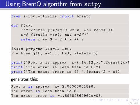
Using BrentQ algorithm from scipy
from scipy.optimize import brentq
def f(x):
""" returns f(x)=x^3-2x^2. Has roots at
x=0 (double root) and x=2"""
return x ** 3 - 2 * x ** 2
#main program starts here
x = brentq(f, a=1.5, b=3, xtol=1e-6)
print("Root x is approx. x={:14.12g}.".format(x))
print("The error is less than 1e-6.")
print("The exact error is {}.".format (2 - x))
generates this:
Root x is approx. x= 2.00000001896.
The error is less than 1e-6.
The exact error is -1.89582864962e-08.
173 / 334

Using fsolve algorithm from scipy
from scipy.optimize import fsolve
# multidimensional solver
def f(x):
""" returns f(x)=x^2-2x^2. Has roots at
x=0 (double root) and x=2"""
return x ** 3 - 2* x ** 2
#main program starts here
x = fsolve(f, x0 =1.6)
print("Root x is approx. x={}.".format(x))
print("The error is less than 1e-6.")
print("The exact error is {}.".format (2 - x[0]))
generates this:
Root x is approx. x=[ 2.].
The error is less than 1e-6.
The exact error is 0.0.174 / 334
Computing derivativesnumerically
175 / 334

Overview
Motivation:
We need derivatives of functions for some optimisationand root finding algorithmsNot always is the function analytically known (but weare usually able to compute the function numerically)The material presented here forms the basis of thefinite-difference technique that is commonly used tosolve ordinary and partial differential equations.
The following slides show
the forward difference techniquethe backward difference technique and thecentral difference technique to approximate thederivative of a function.We also derive the accuracy of each of these methods.
176 / 334

The 1st derivative
(Possible) Definition of the derivative (or “differentialoperator” d
dx)
df
dx(x) = lim
h→0
f(x+ h)− f(x)h
Use difference operator to approximate differentialoperator
f ′(x) =df
dx(x) = lim
h→0
f(x+ h)− f(x)h
≈ f(x+ h)− f(x)h
⇒ can now compute an approximation of f ′ simply byevaluating f .
This is called the forward difference because we use f(x)and f(x+ h).
Important question: How accurate is this approximation?
177 / 334

Accuracy of the forward difference
Formal derivation using the Taylor series of f around x
f(x + h) =
∞∑n=0
hnf (n)(x)
n!
= f(x) + hf ′(x) + h2f ′′(x)
2!+ h3
f ′′′(x)
3!+ . . .
Rearranging for f ′(x)
hf ′(x) = f(x + h)− f(x)− h2f ′′(x)
2!− h3
f ′′′(x)
3!− . . .
f ′(x) =1
h
(f(x + h)− f(x)− h2
f ′′(x)
2!− h3
f ′′′(x)
3!− . . .
)=
f(x + h)− f(x)
h−
h2 f′′(x)2! − h3 f
′′′(x)3!
h− . . .
=f(x + h)− f(x)
h− h
f ′′(x)
2!− h2
f ′′′(x)
3!− . . .
178 / 334
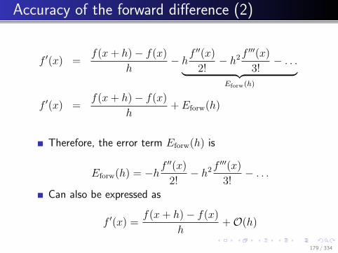
Accuracy of the forward difference (2)
f ′(x) =f(x+ h)− f(x)
h− hf
′′(x)
2!− h2f
′′′(x)
3!− . . .︸ ︷︷ ︸
Eforw(h)
f ′(x) =f(x+ h)− f(x)
h+ Eforw(h)
Therefore, the error term Eforw(h) is
Eforw(h) = −hf ′′(x)
2!− h2f
′′′(x)
3!− . . .
Can also be expressed as
f ′(x) =f(x+ h)− f(x)
h+O(h)
179 / 334
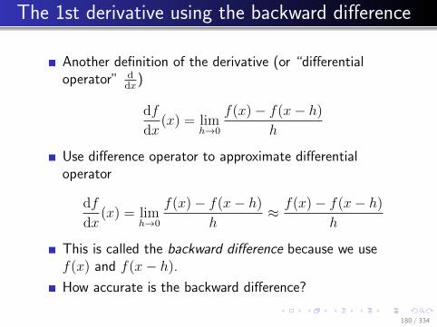
The 1st derivative using the backward difference
Another definition of the derivative (or “differentialoperator” d
dx)
df
dx(x) = lim
h→0
f(x)− f(x− h)h
Use difference operator to approximate differentialoperator
df
dx(x) = lim
h→0
f(x)− f(x− h)h
≈ f(x)− f(x− h)h
This is called the backward difference because we usef(x) and f(x− h).How accurate is the backward difference?
180 / 334

Accuracy of the backward difference
Formal derivation using the Taylor Series of f around x
f(x− h) = f(x)− hf ′(x) + h2f ′′(x)
2!− h3f
′′′(x)
3!+ . . .
Rearranging for f ′(x)
hf ′(x) = f(x)− f(x− h) + h2f ′′(x)
2!− h3
f ′′′(x)
3!− . . .
f ′(x) =1
h
(f(x)− f(x− h) + h2
f ′′(x)
2!− h3
f ′′′(x)
3!− . . .
)=
f(x)− f(x− h)
h+
h2 f′′(x)2! − h3 f
′′′(x)3!
h− . . .
=f(x)− f(x− h)
h+ h
f ′′(x)
2!− h2
f ′′′(x)
3!− . . .
181 / 334

Accuracy of the backward difference (2)
f ′(x) =f(x)− f(x− h)
h+ h
f ′′(x)
2!− h2f
′′′(x)
3!− . . .︸ ︷︷ ︸
Eback(h)
f ′(x) =f(x)− f(x− h)
h+ Eback(h) (7)
Therefore, the error term Eback(h) is
Eback(h) = hf ′′(x)
2!− h2f
′′′(x)
3!− . . .
Can also be expressed as
f ′(x) =f(x)− f(x− h)
h+O(h)
182 / 334

Combining backward and forward differences (1)
The approximations are
forward:
f ′(x) =f(x+ h)− f(x)
h+ Eforw(h) (8)
backward
f ′(x) =f(x)− f(x− h)
h+ Eback(h) (9)
Eforw(h) = −hf′′(x)
2!− h2
f ′′′(x)
3!− h3
f ′′′′(x)
4!− h4
f ′′′′′(x)
5!− . . .
Eback(h) = hf ′′(x)
2!− h2
f ′′′(x)
3!+ h3
f ′′′′(x)
4!− h4
f ′′′′′(x)
5!+ . . .
⇒ Add equations (8) and (9) together, then the error cancelspartly.
183 / 334
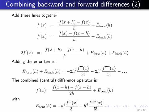
Combining backward and forward differences (2)
Add these lines together
f ′(x) =f(x + h)− f(x)
h+ Eforw(h)
f ′(x) =f(x)− f(x− h)
h+ Eback(h)
2f ′(x) =f(x + h)− f(x− h)
h+ Eforw(h) + Eback(h)
Adding the error terms:
Eforw(h) + Eback(h) = −2h2f ′′′(x)
3!− 2h4
f ′′′′′(x)
5!− . . .
The combined (central) difference operator is
f ′(x) =f(x + h)− f(x− h)
2h+ Ecent(h)
with
Ecent(h) = −h2 f′′′(x)
3!− h4
f ′′′′′(x)
5!− . . .
184 / 334

Central difference
Can be derived (as on previous slides) by adding forwardand backward difference
Can also be interpreted geometrically by defining thedifferential operator as
df
dx(x) = lim
h→0
f(x+ h)− f(x− h)2h
and taking the finite difference form
df
dx(x) ≈ f(x+ h)− f(x− h)
2h
Error of the central difference is only O(h2), i.e. betterthan forward or backward difference
It is generally the case that symmetric differencesare more accurate than asymmetric expressions.
185 / 334
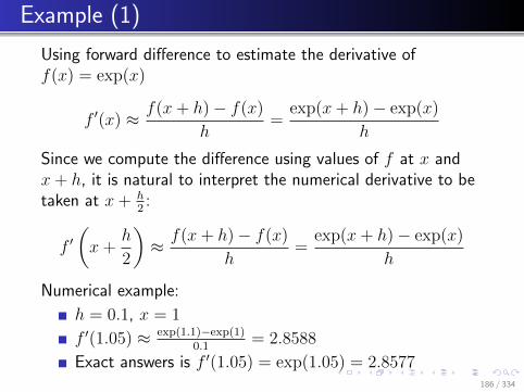
Example (1)
Using forward difference to estimate the derivative off(x) = exp(x)
f ′(x) ≈ f(x+ h)− f(x)h
=exp(x+ h)− exp(x)
h
Since we compute the difference using values of f at x andx+ h, it is natural to interpret the numerical derivative to betaken at x+ h
2:
f ′(x+
h
2
)≈ f(x+ h)− f(x)
h=
exp(x+ h)− exp(x)
h
Numerical example:
h = 0.1, x = 1
f ′(1.05) ≈ exp(1.1)−exp(1)0.1
= 2.8588
Exact answers is f ′(1.05) = exp(1.05) = 2.8577186 / 334

Example (2)
Comparison: forward difference and exact derivative of exp(x)
0 0.5 1 1.5 2 2.5 3 3.50
5
10
15
20
25f(x) = exp(x)
x
exact derivativeforward differences
187 / 334

Summary
Can approximate derivatives of f numerically
need only function evaluations of f
three different difference methods
name formula error
forward f ′(x) = f(x+h)−f(x)h
O(h)backward f ′(x) = f(x)−f(x−h)
hO(h)
central f ′(x) = f(x+h)−f(x−h)2h
O(h2)
central difference is most accurate
Euler’s method (ODE) can be derived from forward difference
Newton’s root finding method can be derived from forward difference
LAB7
188 / 334
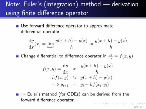
Note: Euler’s (integration) method — derivation
using finite difference operator
Use forward difference operator to approximatedifferential operator
dy
dx(x) = lim
h→0
y(x+ h)− y(x)h
≈ y(x+ h)− y(x)h
Change differential to difference operator in dydx
= f(x, y)
f(x, y) =dy
dx≈ y(x+ h)− y(x)
hhf(x, y) ≈ y(x+ h)− y(x)=⇒ yi+1 = yi + hf(xi, yi)
⇒ Euler’s method (for ODEs) can be derived from theforward difference operator.
189 / 334

Note: Newton’s (root finding) method —
derivation from Taylor series
We are looking for a root, i.e. we are looking for a x so thatf(x) = 0.
We have an initial guess x0 which we refine in subsequent iterations:
xi+1 = xi − hi where hi =f(xi)
f ′(xi). (10)
.
This equation can be derived from the Taylor series of f around x.Suppose we guess the root to be at x and x + h is the actuallocation of the root (so h is unknown and f(x + h) = 0):
f(x + h) = f(x) + hf ′(x) + . . .
0 = f(x) + hf ′(x) + . . .
=⇒ 0 ≈ f(x) + hf ′(x)
⇐⇒ h ≈ − f(x)
f ′(x). (11)
190 / 334

Numpy
191 / 334

numpy
numpy
is an interface to high performance linear algebra libraries(ATLAS, LAPACK, BLAS)
provides
the array objectfast mathematical operations over arrayslinear algebra, Fourier transforms, Random Numbergeneration
Numpy is NOT part of the Python standard library.
192 / 334

numpy arrays (vectors)
An array is a sequence of objects
all objects in one array are of the same type
Here are a few examples:
>>> from numpy import array
>>> a = array([1, 4, 10])
>>> type(a)
<type ’numpy.ndarray ’>
>>> a.shape
(3,)
>>> a ** 2
array ([ 1, 16, 100])
>>> numpy.sqrt(a)
array ([ 1. , 2. , 3.16227766])
>>> a > 3
array ([False , True , True], dtype=bool)
193 / 334

Array creation
Can create from other sequences through array function:
1d-array (vector)
>>> a = array([1, 4, 10])
>>> a
array ([ 1, 4, 10])
>>> print(a)
[ 1 4 10]
2d-array (matrix):
>>> B = array ([[0, 1.5], [10, 12]])
>>> B
array ([[ 0. , 1.5],
[ 10. , 12. ]])
>>> print(B)
[[ 0. 1.5]
[ 10. 12. ]]
194 / 334

Array shape I
The shape is a tuple that describes
(i) the dimensionality of the array (that is the length ofthe shape tuple) and
(ii) the number of elements for each dimension.
Example:
>>> a.shape
(3,)
>>> B.shape
(2, 2)
Can use shape attribute to change shape:
195 / 334

Array shape II
>>> B
array ([[ 0. , 1.5],
[ 10. , 12. ]])
>>> B.shape
(2, 2)
>>> B.shape = (4,)
>>> B
array ([ 0. , 1.5, 10. , 12. ])
196 / 334

Array size
The total number of elements is given through the size
attribute:
>>> a.size
3
>>> B.size
4
The total number of bytes used is given through the nbytes
attribute:
>>> a.nbytes
12
>>> B.nbytes
32
197 / 334
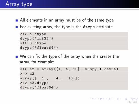
Array type
All elements in an array must be of the same type
For existing array, the type is the dtype attribute
>>> a.dtype
dtype(’int32 ’)
>>> B.dtype
dtype(’float64 ’)
We can fix the type of the array when the create thearray, for example:
>>> a2 = array([1, 4, 10], numpy.float64)
>>> a2
array ([ 1., 4., 10.])
>>> a2.dtype
dtype(’float64 ’)
198 / 334
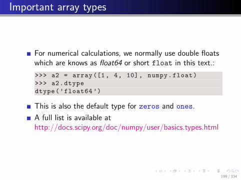
Important array types
For numerical calculations, we normally use double floatswhich are knows as float64 or short float in this text.:
>>> a2 = array([1, 4, 10], numpy.float)
>>> a2.dtype
dtype(’float64 ’)
This is also the default type for zeros and ones.
A full list is available athttp://docs.scipy.org/doc/numpy/user/basics.types.html
199 / 334
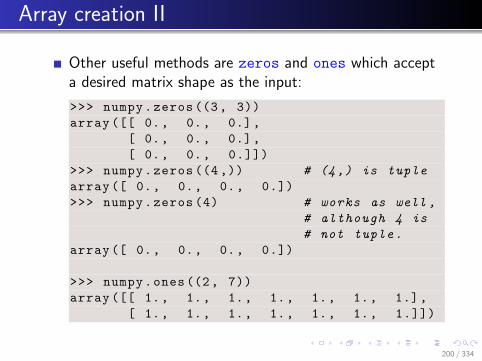
Array creation II
Other useful methods are zeros and ones which accepta desired matrix shape as the input:
>>> numpy.zeros((3, 3))
array ([[ 0., 0., 0.],
[ 0., 0., 0.],
[ 0., 0., 0.]])
>>> numpy.zeros ((4 ,)) # (4,) is tuple
array ([ 0., 0., 0., 0.])
>>> numpy.zeros (4) # works as well ,
# although 4 is
# not tuple.
array ([ 0., 0., 0., 0.])
>>> numpy.ones((2, 7))
array ([[ 1., 1., 1., 1., 1., 1., 1.],
[ 1., 1., 1., 1., 1., 1., 1.]])
200 / 334

Array indexing (1d arrays)
>>> x = numpy.array(range(0, 10, 2))
>>> x
array ([0, 2, 4, 6, 8])
>>> x[3]
6
>>> x[4]
8
>>> x[-1]
Can query length as for any sequence:
>>> len(x)
5
>>> x.shape
(5,)
201 / 334

Array indexing (2d arrays)
>>> C = numpy.arange (12)
>>> C
array ([ 0, 1, 2, 3, 4, 5, 6, 7, 8, 9, 10, 11])
>>> C.shape = (3, 4)
>>> C
array ([[ 0, 1, 2, 3],
[ 4, 5, 6, 7],
[ 8, 9, 10, 11]])
>>> C[0, 0]
0
>>> C[2, 0]
8
>>> C[2, -1]
11
>>> C[-1, -1]
11
202 / 334

Array slicing (1d arrays)
New double colon operator ::: Read as START:END:INDEX
STEP
If either START or END are omitted, the end of the array isused:
>>> y = numpy.arange (10)
>>> y
array ([0, 1, 2, 3, 4, 5, 6, 7, 8, 9])
>>> y[0:5] #slicing as we know it
array ([0, 1, 2, 3, 4])
>>> y[0:5:1] #slicing with index step 1
array ([0, 1, 2, 3, 4])
>>> y[0:5:2] #slicing with index step 2
array ([0, 2, 4])
>>> y[:5:2] #from the beginning
array ([0, 2, 4])
203 / 334

Array slicing (1d arrays continued) continued
Can also use a negative step size:
>>> y[0:5:1] # positive index step size
array ([0, 1, 2, 3, 4])
>>> y[0:5: -1] # negative index step size
array ([], dtype=int32)
>>> y[5:0: -1]
array ([5, 4, 3, 2, 1])
>>> y[5:0: -2]
array ([5, 3, 1])
>>> y[:0: -2]
array ([9, 7, 5, 3, 1])
>>> y[:0: -1]
array ([9, 8, 7, 6, 5, 4, 3, 2, 1])
>>> y[:: -1] # reverses array elements
array ([9, 8, 7, 6, 5, 4, 3, 2, 1, 0])
204 / 334

Creating copies of arrays
Create copy of 1d array:
>>> copy_y = y[:]
Could also use copy y = y[::] to create a copy.To create a copy with reverse order of elements, we can use:
>>> y[:: -1]
array ([9, 8, 7, 6, 5, 4, 3, 2, 1, 0])
To create new array z of the same size as y (filled with zeros,say) we can use (for example):
>>> y
array ([0, 1, 2, 3, 4, 5, 6, 7, 8, 9])
>>> z=numpy.zeros(y.shape)
>>> z
array ([0., 0., 0., 0., 0., 0., 0., 0., 0., 0.])
205 / 334

Array slicing (2d)
Slicing for 2d (or higher dimensional arrays) is analog to 1-dslicing, but applied to each component. Common operationsinclude extraction of a particular row or column from a matrix:
>>> C
array ([[ 0, 1, 2, 3],
[ 4, 5, 6, 7],
[ 8, 9, 10, 11]])
>>> C[0, :] # row with index 0
array ([0, 1, 2, 3])
>>> C[:, 1] # column with index 1
# (i.e. 2nd col)
array ([1, 5, 9])
206 / 334

Other linear algebra tools
help(numpy.linalg) provides an overview, including
pinv to compute the inverse of a matrix
svd to compute a singular value decomposition
det to compute the determinant
eig to compute eigenvalues and eigenvectors
207 / 334

Curve fitting
We typically fit lower order polynomials or other functions(which are the model that we expect the data to follow)through a number of points (often measurements).
We typically have many more points than degrees offreedom, and would employ techniques such as leastsquared fitting.
The function numpy.polyfit provides this functionalityfor polynomials.
The function scipy.optimize.curve fit providescurve fitting for generic functions (not restricted topolynomials).
208 / 334

Solving linear systems of equations
numpy.linealg.solve(A, b) solves Ax = b for asquare matrix A and given vector b, and returns thesolution vector x as an array object:
>>> A=numpy.array ([[1, 0], [0, 2]])
>>> b=numpy.array([1, 4])
>>> from numpy import linalg as LA
>>> x = LA.solve(A, b)
>>> x
array ([ 1., 2.])
>>> numpy.dot(A, x) #Computing A*x
array ([ 1., 4.]) #this should be b
209 / 334

Other comments
numpy provides fast array operations (comparable toMatlab’s matrices)
fast if number of elements is large: for an array with oneelement, numpy.sqrt will be slower than math.sqrt
speed-ups of up to factor 300 are possible using numpyinstead of lists
Consult Numpy documentation if used outside this course.
Matlab users may want to read Numpy for Matlab Users
210 / 334
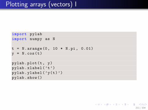
Plotting arrays (vectors) I
import pylab
import numpy as N
t = N.arange(0, 10 * N.pi , 0.01)
y = N.cos(t)
pylab.plot(t, y)
pylab.xlabel(’t’)
pylab.ylabel(’y(t)’)
pylab.show()
211 / 334

Plotting arrays (vectors) II
212 / 334
Matplotlib / Pylab I
Matplotlib tries to make easy things easy and hard thingspossible
a python 2D plotting library which produces publicationquality figures (increasingly also 3d)
can be fully scripted but interactive interface available
Within the IPython console (for example in Spyder), use
%matplotlib inline to see plots inside the consolewindow, and
%matplotlib qt to create pop-up windows with the plotwhen the matplotlib.show() command is used.
213 / 334

Matplotlib / Pylab II
Pylab is a Matlab-like (state-driven) plotting interface (tomatplotlib).
Convenient for ’simple’ plots
Check examples in lecture note text book and
Make use of help(pylab.plot) to remind you of linestyles, symbols etc.
Check gallery athttp://matplotlib.org/gallery.html#pylab examples
Matplotlib.pyplot is an object oriented plotting interface.
Very fine grained control over plots
Check gallery at Matplotlib gallery
Try Matplotlib notebook (on module’s home page) as anintroduction and useful reference.
LAB8214 / 334

Higher Order Functions 2
215 / 334

More list processing and functional programming
So far, have processed lists by iterating through themusing for-loop
perceived to be conceptually simple (by most learners) but
not as compact as possible and not always as fast aspossible
Alternatives:
list comprehensionmap, filter, reduce, often used with lambda
216 / 334
Anonymous function lambda
lambda: anonymous function (function literal)
>>> lambda a: a
<function <lambda > at 0x319c70 >
>>> lambda a: 2 * a
<function <lambda > at 0x319af0 >
>>> (lambda a: 2 * a)
<function <lambda > at 0x319c70 >
>>> (lambda a: 2 * a)(10)
20
>>> (lambda a: 2 * a)(20)
40
>>> (lambda x, y: x + y)(10 ,20)
30
>>> (lambda x, y, z: (x+y) * z )(10 ,20 ,2)
60
>>> type(lambda x, y: x + y)
<type ’function ’>
Useful to define a small helper function that is onlyneeded once 217 / 334

Lambda usage example 1
Integrate f(x) = x2 from 0 to 2, without lambda
lambda1.py :
from scipy.integrate import quad
def f(x):
return x * x
y, abserr = quad(f, 0, 2)
print("Int f(x)=x^2 from 0 to 2 = {:f} +- {:g}"
.format(y, abserr ))
With lambda lambda1b.py :
from scipy.integrate import quad
y, abserr = quad(lambda x: x * x, 0, 2)
print("Int f(x)=x^2 from 0 to 2 = {:f} +- {:g}"
.format(y, abserr ))
Both programs produce the same output:
Int f(x)=x^2 from 0 to 2 = 2.666667 +- 2.96059e-14218 / 334

Higher order functions
Roughly: “Functions that take or return functions” (see forexample (Wikipedia entry))Rough summary (check help(COMMAND) for details)
map(function, sequence) → list:apply function to all elements in sequence
filter(function, sequence) → list:return items of sequence for which function(item) is true.
reduce(function, sequence, initial) → value:apply function(x,y) from left to right to reduce sequenceto a single value.
219 / 334
Map
map(function, sequence) → list: apply function toall elements in sequence
Example:
>>> def f(x): return x ** 2
...
>>> map(f, [0, 1, 2, 3, 4])
[0, 1, 4, 9, 16]
Equivalent operation using list comprehension:
>>> [ x ** 2 for x in [0, 1, 2, 3, 4]]
[0, 1, 4, 9, 16]
220 / 334

Examples map
Example:
>>> import math
>>> map(math.exp , [0 ,0.1 ,0.2 ,1. ,10 ,100])
[1.0, 1.1051709180756477 , 1.2214027581601699 ,
2.7182818284590451 ,22026.465794806718 ,
2.6881171418161356e+43]
Example (slug):
>>> news="Python programming occasionally \
... more fun than expected"
>>> slug = "-".join( map( lambda w: w[0:6],
... news.split ()))
>>> slug
’Python -progra -proves -more -fun -than -expect ’
Equivalent list comprehension expression:
>>> slug = "-".join( [ w[0:6] for w
... in news.split() ])
221 / 334

Filter
filter(function, sequence) → list: return itemsof sequence for which function(item) is true.Example:
>>> c="The quick brown fox jumps".split()
>>> print c
[’The’, ’quick ’, ’brown ’, ’fox’, ’jumps ’]
>>> def len_gr_4(s):
... return len(s) > 4
>>> map( len_gr_4 , c)
[False , True , True , False , True]
>>> filter( len_gr_4 , c)
[’quick ’, ’brown ’, ’jumps ’]
>>> filter( lambda w: len(w) > 4, c)
[’quick ’, ’brown ’, ’jumps ’]
Equivalent operation using list comprehension:
>>> [ s for s in c if len(s)>4 ]
[’quick ’, ’brown ’, ’jumps ’]
222 / 334

Examples filter
Example:
>>> def is_positive(n):
... return n > 0
>>> filter(is_positive ,
... [-5,-4,-3,-2,-1,0,1,2,3,4])
[1, 2, 3, 4]
>>> filter(lambda n:n>0,
... [-5,-4,-3,-2,-1,0,1,2,3,4])
[1, 2, 3, 4]
List comprehension equivalent:
>>> [ x for x in
... [-5,-4,-3,-2,-1,0,1,2,3,4] if x>0]
[1, 2, 3, 4]
223 / 334

Reduce
reduce(function, sequence, initial) → value:apply function(x,y) from left to right to reduce sequenceto a single value.Examples:
>>> def f(x,y):
... print "Called with x={}, y={}".format(x, y)
... return x + y
...
>>> reduce(f, [1, 3, 5], 0)
Called with x=0, y=1
Called with x=1, y=3
Called with x=4, y=5
9
>>> reduce(f, [1, 3, 5], 100)
Called with x=100, y=1
Called with x=101, y=3
Called with x=104, y=5
109224 / 334

Reduce
>>> def f(x,y):
... print "Called with x=%s, y=%s" % (x,y)
... return x+y
...
>>> reduce(f,"test","")
Called with x=, y=t
Called with x=t, y=e
Called with x=te , y=s
Called with x=tes , y=t
’test’
>>> reduce(f,"test","FIRST")
Called with x=FIRST , y=t
Called with x=FIRSTt , y=e
Called with x=FIRSTte , y=s
Called with x=FIRSTtes , y=t
’FIRSTtest ’
225 / 334

Operator module
operator module contains functions which are typicallyaccessed not by name, but via some symbols or specialsyntax.
For example 3 + 4 is equivalent to operator.add(3,
4). Thus:
def f(x, y): return x + y
reduce(f, range (10), 0)
can also be written as:
reduce(operator.add , range (10), 0)
Note: could also use:
reduce(lambda a, b: a + b, range (10), 0)
but use of operator module is preferred (faster).
226 / 334

Functional programming
Functions like map, reduce and filter are found in justabout any lanugage supporting functional programming.
provide functional abstraction for commonly written loops
Use those instead of writing loops, because
Writing loops by hand is quite tedious and error-prone.The functional version is often clearer to read.The functions result in faster code (if you can avoidlambda)
227 / 334
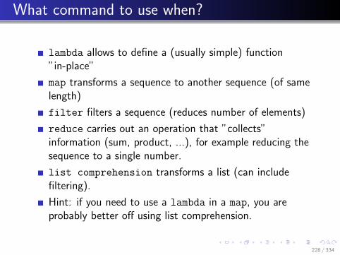
What command to use when?
lambda allows to define a (usually simple) function”in-place”
map transforms a sequence to another sequence (of samelength)
filter filters a sequence (reduces number of elements)
reduce carries out an operation that ”collects”information (sum, product, ...), for example reducing thesequence to a single number.
list comprehension transforms a list (can includefiltering).
Hint: if you need to use a lambda in a map, you areprobably better off using list comprehension.
228 / 334
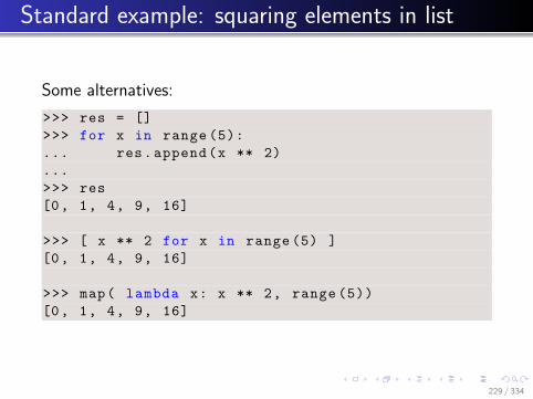
Standard example: squaring elements in list
Some alternatives:
>>> res = []
>>> for x in range (5):
... res.append(x ** 2)
...
>>> res
[0, 1, 4, 9, 16]
>>> [ x ** 2 for x in range (5) ]
[0, 1, 4, 9, 16]
>>> map( lambda x: x ** 2, range (5))
[0, 1, 4, 9, 16]
229 / 334
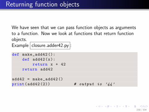
Returning function objects
We have seen that we can pass function objects as argumentsto a function. Now we look at functions that return functionobjects.Example closure adder42.py :
def make_add42 ():
def add42(x):
return x + 42
return add42
add42 = make_add42 ()
print(add42 (2)) # output is ’44’
230 / 334
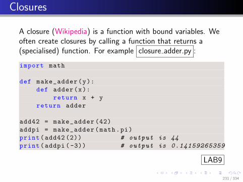
Closures
A closure (Wikipedia) is a function with bound variables. Weoften create closures by calling a function that returns a(specialised) function. For example closure adder.py :
import math
def make_adder(y):
def adder(x):
return x + y
return adder
add42 = make_adder (42)
addpi = make_adder(math.pi)
print(add42 (2)) # output is 44
print(addpi (-3)) # output is 0.14159265359
LAB9
231 / 334
Object Orientation and all that
232 / 334
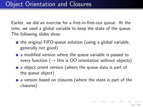
Object Orientation and Closures
Earlier, we did an exercise for a first-in-first-out queue. At thetime, we used a global variable to keep the state of the queue.The following slides show:
the original FIFO-queue solution (using a global variable,generally not good)
a modified version where the queue variable is passed toevery function (→ this is OO orientation without objects)
a object orient version (where the queue data is part ofthe queue object)
a version based on closures (where the state is part of theclosures)
233 / 334
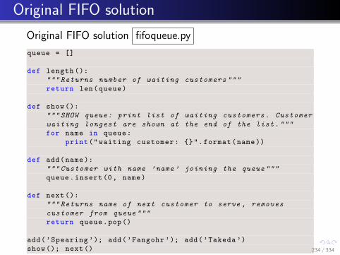
Original FIFO solution
Original FIFO solution fifoqueue.py
queue = []
def length ():
""" Returns number of waiting customers """
return len(queue)
def show ():
""" SHOW queue: print list of waiting customers . Customer
waiting longest are shown at the end of the list."""
for name in queue:
print("waiting customer: {}".format(name))
def add(name):
""" Customer with name ’name ’ joining the queue """
queue.insert(0, name)
def next ():
""" Returns name of next customer to serve , removes
customer from queue """
return queue.pop()
add(’Spearing ’); add(’Fangohr ’); add(’Takeda ’)
show (); next() 234 / 334

Improved FIFO solution
Improved FIFO solution fifoqueue2.py
def length(queue ):
return len(queue)
def show(queue):
for name in queue:
print("waiting customer: {}".format(name))
def add(queue , name):
queue.insert(0, name)
def next(queue):
return queue.pop()
q1 = []
q2 = []
add(q1 , ’Spearing ’); add(q1, ’Fangohr ’); add(q1 , ’Takeda ’)
add(q2 , ’John’); add(q2, ’Peter’)
print("{} customers in queue1:".format(length(q1)); show(q1)
print("{} customers in queue2:".format(length(q2)); show(q2)
235 / 334

Object-Oriented FIFO solution
Object-Oriented improved FIFO solution fifoqueueOO.py
class Fifoqueue:
def __init__(self):
self.queue = []
def length(self):
return len(self.queue)
def show(self):
for name in self.queue:
print("waiting customer: {}".format(name))
def add(self , name):
self.queue.insert(0, name)
def next(self):
return self.queue.pop()
q1 = Fifoqueue ()
q2 = Fifoqueue ()
q1.add(’Spearing ’); q1.add(’Fangohr ’); q1.add(’Takeda ’)
q2.add(’John’); q2.add(’Peter ’)
print("{} customers in queue1:".format(q1.length ()); q1.show()
print("{} customers in queue2:".format(q2.length ()); q2.show()236 / 334

Functional FIFO solution
Functional (closure-based) FIFO solution fifoqueue closure.py
def make_queue ():
queue = []
def length ():
return len(queue)
def show ():
for name in queue: print("waiting customer: {}".format(name))
def add(name):
queue.insert(0, name)
def next ():
return queue.pop()
return add , next , show , length
q1_add , q1_next , q1_show , q1_length = make_queue ()
q2_add , q2_next , q2_show , q2_length = make_queue ()
q1_add(’Spearing ’); q1_add(’Fangohr ’); q1_add(’Takeda ’)
q2_add(’John’); q2_add(’Peter ’)
print("{} customers in queue1:".format(q1_length ()); q1_show ()
print("{} customers in queue2:".format(q2_length ()); q2_show ()237 / 334
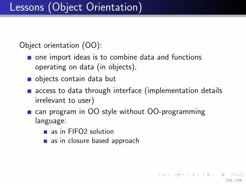
Lessons (Object Orientation)
Object orientation (OO):
one import ideas is to combine data and functionsoperating on data (in objects),
objects contain data but
access to data through interface (implementation detailsirrelevant to user)
can program in OO style without OO-programminglanguage:
as in FIFO2 solutionas in closure based approach
238 / 334

Numerical Integration
239 / 334

Numerical Integration 1— Overview
Different situations where we use integration:
(A) solving (definite) integrals
(B) solving (ordinary) differential equations
more complicated than (A)Euler’s method, Runge-Kutta methods
Both (A) and (B) are important.
We begin with the numeric computation of integrals (A).
240 / 334

(A) Definite Integrals
Often written as
I =
b∫a
f(x)dx (12)
example: I =2∫0
exp(−x2)dx
solution is I ∈ R (i.e. a number)
right hand side f(x) depends only on xif f(x) > 0 ∀x ∈ [a, b], then we can visualise I as thearea underneath f(x)
Note that the integral is not necessarily the same as thearea enclosed by f(x) and the x-axis:
2π∫0
sin(x)dx = 0
1∫0
(−1)dx = −1
241 / 334

(B) Ordinary Differential Equations (ODE)
Often written as
y′ ≡ dy
dx= f(x, y) (13)
example: dvdt
= 1m(g − cv2)
solution isy(x) : R→ R
x 7→ y(x)(i.e. a function)
right hand side f(x, y) depends on x and on solution y
Can write (13) formally as y =∫ dydxdx =
∫f(x, y)dx. That’s
why we “integrate differential equations” to solve them.
242 / 334

Numeric computation of definite integrals
Example:
I =
2∫0
exp(−x2)dx
0 0.5 1 1.5 2x
0
0.2
0.4
0.6
0.8
1
f(x) = exp( -x2)
243 / 334

Simple trapezoidal rule
Approximate function by straight line
0 0.5 1 1.5 2x
0
0.2
0.4
0.6
0.8
1
f(x) = exp( -x2)trapezoidal approximation
244 / 334
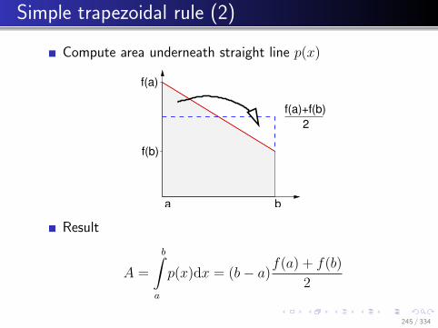
Simple trapezoidal rule (2)
Compute area underneath straight line p(x)
f(a)+f(b) 2
ba
f(b)
f(a)
Result
A =
b∫a
p(x)dx = (b− a)f(a) + f(b)
2
245 / 334

Simple trapezoidal rule (3)
Aim: compute
I =
b∫a
f(x)dx
Strategy:
approximate f(x) with a linear function p(x):
p(x) ≈ f(x)
compute the area A underneath that function p(x):
A =
b∫a
p(x)dx = (b− a)f(a) + f(b)
2
approximate
I =
b∫a
f(x)dx ≈b∫
a
p(x)dx = A = (b− a)f(a) + f(b)
2
246 / 334

Simple trapezoidal rule (4) Example
Integrate f(x) = x2
I =
2∫0
x2dx
What is the (correct) analytical answer?Integrating polynomials:
I =
b∫a
xkdx =
[1
k + 1xk+1
]ba
for a = 0 and b = 2 and k = 2
I =
[1
2 + 1x2+1
]20
=1
323 =
8
3≈ 2.6667
247 / 334

Using the trapezoidal rule
A = (b− a)f(a) + f(b)
2= 2
0 + 4
2= 4
The correct answer is I = 8/3 and the approximation is A = 4.
We thus overestimate I by A−II ≈ 50%.
Plotting f(x) = x2 together with the approximation reveals why weoverestimate I
0 0.5 1 1.5 2x
0
1
2
3
4f(x) = x^2trapezoidal approximation p(x)
The linear approximation, p(x), overestimates f(x) everywhere(except at x = a and x = b).
Therefore, the integral of p(x) is greater than the integral of f(x).
(More formally: f(x) is convex on [a, b] ⇐⇒ f ′′(x) ≥ 0 ∀x ∈ [a, b].)
248 / 334
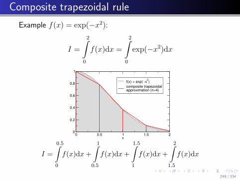
Composite trapezoidal rule
Example f(x) = exp(−x2):
I =
2∫0
f(x)dx =
2∫0
exp(−x2)dx
0 0.5 1 1.5 2x
0
0.2
0.4
0.6
0.8
1
f(x) = exp( -x2)composite trapezoidalapproximation (n=4)
I =
0.5∫0
f(x)dx +
1∫0.5
f(x)dx +
1.5∫1
f(x)dx +
2∫1.5
f(x)dx
249 / 334
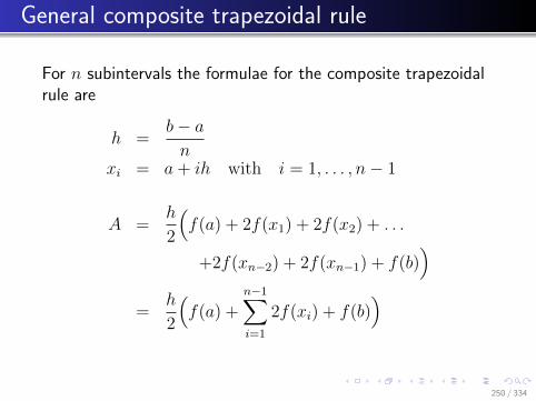
General composite trapezoidal rule
For n subintervals the formulae for the composite trapezoidalrule are
h =b− an
xi = a+ ih with i = 1, . . . , n− 1
A =h
2
(f(a) + 2f(x1) + 2f(x2) + . . .
+2f(xn−2) + 2f(xn−1) + f(b))
=h
2
(f(a) +
n−1∑i=1
2f(xi) + f(b))
250 / 334

Error of composite trapezoidal rule
One of the important (and difficult) questions in numerical analysisand computing is:
How accurate is my approximation?
For integration methods, we are interest in how much the errordecreases when we decrease h (by increasing the number ofsubintervals, n).
For the composite trapezoidal rule it can be shown that:
b∫a
f(x)dx =h
2
(f(a) + f(b) + 2
n−1∑i=1
f(xi)
)+O(h2)
The symbol O(h2) means that the error term is (smaller or equal toan upper bound which is) proportional to h2:
If we take 10 times as many subintervals then h becomes 10times smaller (because h = b−a
n) and the error becomes 100
times smaller (because 1102
= 1100
).
251 / 334

Error of composite trapezoidal rule, example
The table below shows how the error of theapproximation, A, decreases with increasing n for
I =
2∫0
x2dx.
n h A I ∆ = A–I rel.err.=∆/I1 2.000000 4.000000 2.666667 1.333333 50.0000%2 1.000000 3.000000 2.666667 0.333333 12.5000%3 0.666667 2.814815 2.666667 0.148148 5.5556%4 0.500000 2.750000 2.666667 0.083333 3.1250%5 0.400000 2.720000 2.666667 0.053333 2.0000%6 0.333333 2.703704 2.666667 0.037037 1.3889%7 0.285714 2.693878 2.666667 0.027211 1.0204%8 0.250000 2.687500 2.666667 0.020833 0.7813%9 0.222222 2.683128 2.666667 0.016461 0.6173%10 0.200000 2.680000 2.666667 0.013333 0.5000%50 0.040000 2.667200 2.666667 0.000533 0.0200%100 0.020000 2.666800 2.666667 0.000133 0.0050%
The accuracy we actually require depends on the problemunder investigation – no general statement is possible.
252 / 334

Summary trapezoidal rule for numerical integration
Aim: to find an approximation of
I =
b∫a
f(x)dx
Simple trapezoidal method:
approximate f(x) by a simpler (linear) function p(x) andintegrate the approximation p(x) exactly.
Composite trapezoidal method:
divides the interval [a, b] into n equal subintervalsemploys the simple trapezoidal method for eachsubintervalhas an error term of order h2.
253 / 334
Numpy usage examples
254 / 334

Making calculations fast with numpy
Calculations using numpy are faster (up to about 300times) than using pure Python (see example next slide).
Imagine we need to compute the mexican hat functionwith many points
255 / 334

Making calculations fast with numpy I
""" Demo: practical use of numpy (mexhat -numpy.py)"""
import time
import math
import numpy as np
N = 10000
def mexhat_py(t, sigma =1):
""" Computes Mexican hat shape , see
http :// en.wikipedia.org/wiki/ Mexican_hat_wavelet for
equation (13 Dec 2011) """
c = 2. / math.sqrt(3 * sigma) * math.pi ** 0.25
return c * (1 - t ** 2 / sigma ** 2) * \
math.exp(-t ** 2 / (2 * sigma ** 2))
def mexhat_np(t, sigma =1):
""" Computes Mexican hat shape using numpy , see
http :// en.wikipedia.org/wiki/ Mexican_hat_wavelet for
equation (13 Dec 2011) """
256 / 334

Making calculations fast with numpy II
c = 2. / math.sqrt(3 * sigma) * math.pi ** 0.25
return c * (1 - t ** 2 / sigma ** 2) * \
np.exp(-t ** 2 / (2 * sigma ** 2))
def test_is_really_the_same ():
""" Checking whether mexhat_np and mexhat_py produce
the same results."""
xs1 , ys1 = loop1()
xs2 , ys2 = loop2()
deviation = math.sqrt(sum((ys1 - ys2) ** 2))
print "error:", deviation
assert deviation < 1e-15
def loop1 ():
""" Compute arrays xs and ys with mexican hat function
in ys(xs), returns tuple (xs ,ys)"""
xs = np.linspace(-5, 5, N)
ys = []
for x in xs:
ys.append(mexhat_py(x))
return xs, ys
257 / 334

Making calculations fast with numpy III
def loop2 ():
""" As loop1 , but uses numpy to be faster."""
xs = np.linspace(-5, 5, N)
return xs, mexhat_np(xs)
def time_this(f):
""" Call f, measure and return number of seconds
execution of f() takes """
starttime = time.time()
f()
stoptime = time.time()
return stoptime - starttime
def make_plot(filenameroot ):
import pylab
pylab.figure(figsize =(6, 4))
xs, ys = loop2 ()
pylab.plot(xs, ys , label=’Mexican hat function ’)
pylab.legend ()
258 / 334
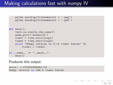
Making calculations fast with numpy IV
pylab.savefig(filenameroot + ’.png’)
pylab.savefig(filenameroot + ’.pdf’)
def main ():
test_is_really_the_same ()
make_plot(’mexhat1d ’)
time1 = time_this(loop1)
time2 = time_this(loop2)
print "Numpy version is %.1f times faster" %\
(time1 / time2)
if __name__ == "__main__":
main()
Produces this output:
error: 1.57009245868e-16
Numpy version is 248.4 times faster
259 / 334

Making calculations fast with numpy V
A lot of the source code above is focussed on measuring theexecution time. Within IPython, we could just have used%timeit loop1 and %timeit loop2 to get to the sametiming information.
260 / 334

Array objects of shape () behave like scalars I
>>> import numpy as np
>>> np.sqrt (4.) #apply numpy -sqrt to scalar
2.0 # looks like float
>>> type(np.sqrt (4.)) # but is numpy -float
<type ’numpy.float64 ’>
>>> float(np.sqrt (4.)) #but can convert to float
2.0
>>> a = np.sqrt (4.) # what shape is the
# numpy -float?
>>> a.shape
()
>>> type(a) # just to remind us
<type ’numpy.float64 ’> # of the type
>>>
So numpy-scalars (i.e. arrays with shape ()) can be convertedto float. In fact, this happens implicitly:
261 / 334

Array objects of shape () behave like scalars II
>>> import numpy as np
>>> import math
>>> math.sqrt(np.sqrt (81))
3.0
Conversion to float fails if array has more than one element:
>>> import numpy as np
>>> a = np.array ([10., 20., 30.])
>>> a
array ([ 10., 20., 30.])
>>> print(a)
[ 10. 20. 30.]
>>> type(a)
<type ’numpy.ndarray ’>
>>> a.shape
(3,)
>>> float(a)
Traceback (most recent call last):
262 / 334
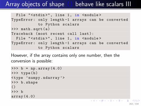
Array objects of shape () behave like scalars III
File "<stdin >", line 1, in <module >
TypeError: only length -1 arrays can be converted
to Python scalars
>>> math.sqrt(a)
Traceback (most recent call last):
File "<stdin >", line 1, in <module >
TypeError: only length -1 arrays can be converted
to Python scalars
However, if the array contains only one number, then theconversion is possible:
>>> b = np.array (4.0)
>>> type(b)
<type ’numpy.ndarray ’>
>>> b.shape
()
>>> b
array (4.0)
263 / 334

Array objects of shape () behave like scalars IV
>>> float(b)
4.0
>>> math.sqrt(b)
2.0
Note: an array with shape (1,) can also be converted to afloat:
>>> c = np.array ([3])
>>> c.shape
(1,)
>>> float(c)
3.0
This allows us to write functions f(x) that can take an inputargument x which can either be a numpy.array or a scalar.The mexhat np(t) function is such an example:
264 / 334

Array objects of shape () behave like scalars V
>>> a = mexhat_np (3.)
>>> type(a)
<type ’numpy.float64 ’> #essentially a float
>>> a
-0.13662231969702732
>>> float(a) #converts to python float
-0.13662231969702732
>>> b = mexhat_np(np.arange(0, 11, 2))
>>> type(b)
<type ’numpy.ndarray ’>
>>> b
array ([ 1.53729366e+00, -6.24150219e-01,
-7.73556857e-03, -8.19453296e-07,
-1.22651811e-12, -2.93540437e -20])
265 / 334

Scientific Python
266 / 334

SciPy (SCIentific PYthon)
(Partial) output of help(scipy):
stats --- Statistical Functions
sparse --- Sparse matrix
lib --- Python wrappers to external
libraries
linalg --- Linear algebra routines
signal --- Signal Processing Tools
misc --- Various utilities that don’t
have another home.
interpolate --- Interpolation Tools
optimize --- Optimization Tools
cluster --- Vector Quantization / Kmeans
fftpack --- Discrete Fourier Transform
io --- Data input and output
integrate --- Integration routines
lib.lapack --- Wrappers to LAPACK library
special --- Special Functions
lib.blas --- Wrappers to BLAS library
267 / 334

Interpolation of data
Given a set of N points (xi, yi) with i = 1, 2, . . . N , wesometimes need a function f̂(x) which returns yi = f(xi) andinterpolates the data between the xi.
→ y0 = scipy.interpolate.interp1d(x,y) doesthis interpolation. Note that the function
interp1d returns a function y0 which will interpolate thex-y data for any given x when called as y0(x)
Data interpolation of yi = f(xi) may be useful toCreate smoother plots of f(x)find minima/maxima of f(x)find xc so that f(xc) = yc, provide inverse functionx = f−1(y)integrate f(x)
Need to decide how to interpolate (nearest, linear,quadratic or cubic splines, ...)
268 / 334

Interpolation of data example I
import numpy as np
import scipy.interpolate
import pylab
def create_data(n):
""" Given an integer n, returns n data points
x and values y as a numpy.array."""
xmax = 5.
x = np.linspace(0, xmax , n)
y = - x**2
#make x-data somewhat irregular
y += 1.5 * np.random.normal(size=len(x))
return x, y
#main program
n = 10
x, y = create_data(n)
#use finer and regular mesh for plot
xfine = np.linspace (0.1, 4.9, n * 100)
# interpolate with piecewise constant function (p=0)
y0 = scipy.interpolate.interp1d(x, y, kind=’nearest ’)
269 / 334

Interpolation of data example II
# interpolate with piecewise linear func (p=1)
y1 = scipy.interpolate.interp1d(x, y, kind=’linear ’)
# interpolate with piecewise constant func (p=2)
y2 = scipy.interpolate.interp1d(x, y, kind=’quadratic ’)
pylab.plot(x, y, ’o’, label=’data point’)
pylab.plot(xfine , y0(xfine), label=’nearest ’)
pylab.plot(xfine , y1(xfine), label=’linear ’)
pylab.plot(xfine , y2(xfine), label=’cubic ’)
pylab.legend ()
pylab.xlabel(’x’)
pylab.savefig(’interpolate.pdf’)
pylab.show()
270 / 334

Interpolation of data example III
0 1 2 3 4 5x
30
25
20
15
10
5
0
5
data pointnearestlinearcubic
271 / 334

Curve fitting example I
import numpy as np
import scipy.optimize
import pylab
def create_data(n):
""" Given an integer n, returns n data points
x and values y as a numpy.array."""
xmax = 5.
x = np.linspace(0, xmax , n)
y = - x**2
#make x-data somewhat irregular
y += 1.5 * np.random.normal(size=len(x))
return x, y
def model(x, a, b, c): # Equation for fit
return a * x ** 2 + b * x + c
272 / 334

Curve fitting example II
# main program
n = 10
x, y = create_data(n)
# do curve fit
p, pcov = scipy.optimize.curve_fit(model , x, y)
a, b, c = p
# plot fit and data
xfine = np.linspace (0.1, 4.9, n * 5)
pylab.plot(x, y, ’o’, label=’data point ’)
pylab.plot(xfine , model(xfine , a, b, c), \
label=’fit’)
pylab.title(’fit parameters (a,b,c)=%s’ % p)
pylab.legend ()
pylab.xlabel(’x’)
pylab.savefig(’curvefit2.pdf’)
pylab.show()
273 / 334

Curve fitting example III
0 1 2 3 4 5x
30
25
20
15
10
5
0
5fit parameters (a,b,c)=[-1.06323629 -0.10252473 0.54071275]
data pointfit
274 / 334

Function integration example I
from math import cos , exp , pi
from scipy.integrate import quad
#function we want to integrate
def f(x):
return exp(math.cos(-2 * x * pi)) + 3.2
#call quad to integrate f from -2 to 2
res , err = quad(f, -2, 2)
print("The numerical result is {:f} (+-{:g})"
.format(res , err))
which produces this output:
The numerical result is 17.864264 (+ -1.55117e-11)
LAB10
275 / 334
Optimisation (Minimisation)
Optimisation typically described as:given a function f(x), find xm so that f(xm) is the(local) minimum of f .
To maximise f(x), create a second functiong(x) = −f(x) and minimise g(x).
Optimisation algorithms need to be given a starting point(initial guess x0 as close as possible to xm)
Minimum position x obtained may be local (not global)minimum
276 / 334

Optimisation example I
from scipy import arange , cos , exp
from scipy.optimize import fmin
import pylab
def f(x):
return cos(x) - 3 * exp( -(x - 0.2) ** 2)
# find minima of f(x),
# starting from 1.0 and 2.0 respectively
minimum1 = fmin(f, 1.0)
print "Start search at x=1., minimum is",minimum1
minimum2 = fmin(f, 2.0)
print "Start search at x=2., minimum is",minimum2
# plot function
x = arange(-10, 10, 0.1)
y = f(x)
277 / 334

Optimisation example II
pylab.plot(x, y, label=’$\cos(x)-3e^{-(x -0.2)^2}$’)
pylab.xlabel(’x’)
pylab.grid()
pylab.axis([-5, 5, -2.2, 0.5])
# add minimum1 to plot
pylab.plot(minimum1 , f(minimum1), ’vr’,
label=’minimum 1’)
# add start1 to plot
pylab.plot (1.0, f(1.0) , ’or’, label=’start 1’)
#add minimum2 to plot
pylab.plot(minimum2 ,f(minimum2),’vg’,\
label=’minimum 2’)
#add start2 to plot
pylab.plot (2.0,f(2.0) ,’og’,label=’start 2’)
pylab.legend(loc=’lower left’)
278 / 334
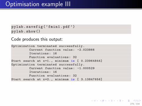
Optimisation example III
pylab.savefig(’fmin1.pdf’)
pylab.show()
Code produces this output:
Optimization terminated successfully.
Current function value: -2.023866
Iterations: 16
Function evaluations: 32
Start search at x=1., minimum is [ 0.23964844]
Optimization terminated successfully.
Current function value: -1.000529
Iterations: 16
Function evaluations: 32
Start search at x=2., minimum is [ 3.13847656]
279 / 334

Optimisation example IV
4 2 0 2 4x
2.0
1.5
1.0
0.5
0.0
0.5
cos(x)−3e−(x−0.2)2
minimum 1start 1minimum 2start 2
LAB11 280 / 334

Ordinary Differential Equations(ODEs)
281 / 334
Ordinary Differential Equations I
Many processes, in particular time-dependent processes,can be described as Ordinary Differential Equations(ODEs). This includes dynamics of engineering systems,quantum physics, chemical reactions, biological systemsmodelling, population dynamics, and many other models.
ODEs have exactly one independent variable, and weassume for simplicity this is the time t.
The easiest ODE type has one degree of freedom, y,which depends on the time t, i.e. y = y(t). (Thinks oftemperature as a function of time, the distance a car hasmoved as function of time, the angular velocity of arotating motor, etc.)
282 / 334

Ordinary Differential Equations II
(In general, a vector y with k components can depend onthe independent variable, in which case we are looking ata system of ordinary differential equations with k degreesof freedom.)
We are seeking the function y(t) – this is the solution ofthe ODE.
We are typically being given an initial value y0 of y(t) atsome time t0 and
the ODE itself which relates the change of y with t tosome function f(t, y), i.e.
dy
dt= f(y, t) (14)
283 / 334

Interface odeint
aim: solvedy
dt= f(y, t)
get access to “odeint”:from scipy.integrate import odeint
odeint has the following input and output parameters:
ys = odeint(f, y0 , ts)
Input:
f is function f(y, t) that returns the right-hand sidey0 is the initial value of the solution at time t0ts is a numpy array containing times ti for which wewould like to know the solution y(ti)
the first value in the array has to be t0 (with y(t0) = y0)
Output:
ys is the numpy array that contains the solution
284 / 334

Using odeint – example 1
require solution y(t) from t = 0 to t = 2dy
dt= −2y with y(0) = 17
import numpy as np
from scipy.integrate import odeint
def f(y,t):
return -2 * y
ts = np.arange(0, 2.1, 0.1)
y0 = 17
ys = odeint(f, y0 , ts)
import pylab
pylab.plot(ts, ys, ’x’)
pylab.grid()
pylab.savefig(’odeintexample1.pdf’)
pylab.show()285 / 334

Using odeint – example 1
Solution:
286 / 334

Using odeint – example 2
require solution y(t) from t = 0 to t = 2dy
dt= − 1
100y + sin(10πt) with y(0) = −2
import math
import numpy as np
from scipy.integrate import odeint
def f(y, t):
return -0.01 * y + \
math.sin (10 * math.pi * t)
ts = np.arange(0, 2.01, 0.01)
y0 = -2
ys = odeint(f, y0 , ts)
import pylab
pylab.plot(ts, ys)
pylab.savefig(’odeintexample2.pdf’)
pylab.show() 287 / 334
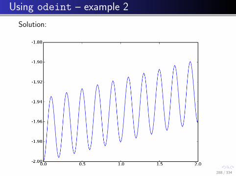
Using odeint – example 2
Solution:
288 / 334
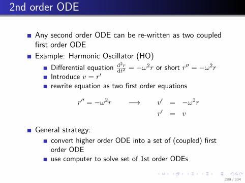
2nd order ODE
Any second order ODE can be re-written as two coupledfirst order ODE
Example: Harmonic Oscillator (HO)
Differential equation d2rdt2
= −ω2r or short r′′ = −ω2rIntroduce v = r′
rewrite equation as two first order equations
r′′ = −ω2r −→ v′ = −ω2r
r′ = v
General strategy:
convert higher order ODE into a set of (coupled) firstorder ODEuse computer to solve set of 1st order ODEs
289 / 334
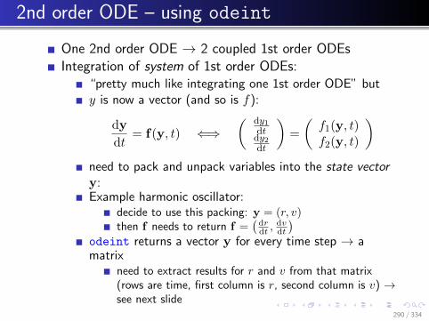
2nd order ODE – using odeint
One 2nd order ODE → 2 coupled 1st order ODEsIntegration of system of 1st order ODEs:
“pretty much like integrating one 1st order ODE” buty is now a vector (and so is f):
dy
dt= f(y, t) ⇐⇒
( dy1dtdy2dt
)=
(f1(y, t)f2(y, t)
)need to pack and unpack variables into the state vectory:Example harmonic oscillator:
decide to use this packing: y = (r, v)then f needs to return f =
(drdt ,
dvdt
)odeint returns a vector y for every time step → amatrix
need to extract results for r and v from that matrix(rows are time, first column is r, second column is v) →see next slide
290 / 334

2nd order ODE – Python solution HO
from numpy import array , arange
from scipy.integrate import odeint
def f(y, t): # right hand side , takes array (!) y
omega = 1
r = y[0] # extract r from array y
v = y[1] # extract v from array y
drdt = v # compute right hand side
dvdt = -omega ** 2 * r
return array ([drdt , dvdt]) # return array
ts = arange(0, 20, 0.1) # required times for solution
r0 = 1 # initial r
v0 = 0 # initial v
y0 = array ([r0, v0]) # combine r and v into y
ys = odeint(f, y0 , ts) # solve ODEs
rs = ys[:, 0] # extract results: r(t)
vs = ys[:, 1] # extract results: v(t)
import pylab # plot results
pylab.plot(ts, rs , label=’r(t)’)
pylab.plot(ts, vs , label=’v(t)’); pylab.legend ()
pylab.savefig(’odeintexample1dHO.pdf’)
pylab.show()291 / 334

2nd order ODE – result
Solution (not annotated):
292 / 334

Summary 2nd order system
Strategy:
transform one 2nd order ODE into 2 (coupled) firstorder ODEssolve both first order ODEs simultaneously
nothing conceptually complicated
but need to use matrices (“arrays”) in Python to shufflethe data around.
Warning: the meaning of y, x depends on context: oftenx = t and y = x. It helps to write down equations beforecoding them.
Use example on previous slides as guidance.
293 / 334
2 Coupled ODEs: Predator-Prey problem I
Predator and prey. Let
p1(t) be the number of rabbitsp2(t) be the number of foxes
Time dependence of p1 and p2:
Assume that rabbits proliferate at a rate a. Per unittime a number ap1 of rabbits is born.Number of rabbits is reduced by collisions with foxes.Per unit time cp1p2 rabbits are eaten.Assume that birth rate of foxes depends only on foodintake in form of rabbits.Assume that foxes die a natural death at a rate b.
Numbers
rabbit birth rate a = 0.7rabbit-fox-collision rate c = 0.007fox death rate b = 1
294 / 334

Predator-Prey problem (2) I
Put all together in predator-prey ODEs
p′1 = ap1 − cp1p2p′2 = cp1p2 − bp2
Solve for p1(0) = 70 and p2(0) = 50 for 30 units of time:
import numpy as N
from scipy.integrate import odeint
def rhs(y, t):
a = 0.7; c = 0.007; b = 1
p1 = y[0]
p2 = y[1]
dp1dt = a * p1 - c * p1 * p2
dp2dt = c * p1 * p2 - b * p2
return N.array([ dp1dt , dp2dt ])
295 / 334
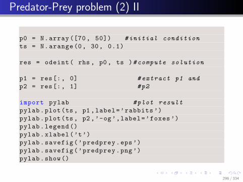
Predator-Prey problem (2) II
p0 = N.array ([70, 50]) #initial condition
ts = N.arange(0, 30, 0.1)
res = odeint( rhs , p0 , ts )#compute solution
p1 = res[:, 0] #extract p1 and
p2 = res[:, 1] #p2
import pylab #plot result
pylab.plot(ts, p1,label=’rabbits ’)
pylab.plot(ts, p2,’-og’,label=’foxes ’)
pylab.legend ()
pylab.xlabel(’t’)
pylab.savefig(’predprey.eps’)
pylab.savefig(’predprey.png’)
pylab.show()
296 / 334

Predator-Prey problem (2) III
297 / 334

Outlook I
Suppose we want to solve a (vector) ODE based onNewton’s equation of motion in three dimensions:
d2r
dt2=
F(r,v, t)
m
Rewrite as two first order (vector) ODEs:
dv
dt=
F(r,v, t)
mdr
dt= v
Need to pack 6 variables into “y”: for example
y = (rx, ry, rz, vx, vy, vz)
298 / 334
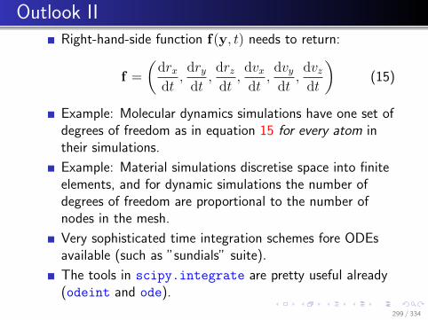
Outlook IIRight-hand-side function f(y, t) needs to return:
f =
(drxdt,drydt,drzdt,dvxdt
,dvydt,dvzdt
)(15)
Example: Molecular dynamics simulations have one set ofdegrees of freedom as in equation 15 for every atom intheir simulations.
Example: Material simulations discretise space into finiteelements, and for dynamic simulations the number ofdegrees of freedom are proportional to the number ofnodes in the mesh.
Very sophisticated time integration schemes fore ODEsavailable (such as ”sundials” suite).
The tools in scipy.integrate are pretty useful already(odeint and ode).
299 / 334

Symbolic Python (sympy)
300 / 334

Symbolic Python I
>>> import sympy
>>> x = sympy.Symbol(’x’) # define symbolic
>>> y = sympy.Symbol(’y’) # variables
>>> x + x
2*x
>>> t = (x + y)**2
>>> print t
(x + y)**2
>>> sympy.expand(t)
x**2 + 2*x*y + y**2
>>> sympy.pprint(t) #PrettyPRINT
2
(x + y)
>>> sympy.printing.latex(t) #Latex export
’\\left(x + y\\ right )^{2}’
301 / 334

Symbolic Python II
>>> t
(x + y)**2
>>> t.subs(x, 3) #substituting variables
(y + 3)**2 #or values
>>> t.subs(x, 3). subs(y, 1)
16
>>> n=t.subs(x, 3). subs(y, sympy.pi)
>>> print n
(3 + pi)**2
>>> n.evalf() #evaluate to float
37.7191603226281
>>> p = sympy.pi
>>> p
pi
>>> p.evalf()
3.14159265358979
>>> p.evalf (47) #request 47 digits
3.1415926535897932384626433832795028841971693993
302 / 334
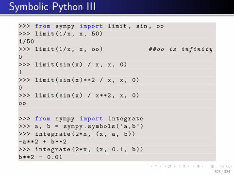
Symbolic Python III
>>> from sympy import limit , sin , oo
>>> limit (1/x, x, 50)
1/50
>>> limit (1/x, x, oo) ##oo is infinity
0
>>> limit(sin(x) / x, x, 0)
1
>>> limit(sin(x)**2 / x, x, 0)
0
>>> limit(sin(x) / x**2, x, 0)
oo
>>> from sympy import integrate
>>> a, b = sympy.symbols(’a,b’)
>>> integrate (2*x, (x, a, b))
-a**2 + b**2
>>> integrate (2*x, (x, 0.1, b))
b**2 - 0.01
303 / 334

Symbolic Python IV
>>> integrate (2*x, (x, 0.1, 2))
3.99000000000000
>>> from sympy import series
>>> taylorseries = series(sin(x), x, 0)
>>> taylorseries
x - x**3/6 + x**5/120 + O(x**6)
>>> sympy.pprint(taylorseries)
3 5
x x
x - -- + --- + O(x**6)
6 120
>>> taylorseries = series(sin(x), x, 0, n=10)
>>> sympy.pprint(taylorseries)
3 5 7 9
x x x x
x - -- + --- - ---- + ------ + O(x**10)
6 120 5040 362880
304 / 334

Symbolic Python V
Finally, we can solve non-linear equations, for example:
>>> (x + 2)*(x - 3) # define quadratic equation
# with roots x=-2, x=3
(x - 3)*(x + 2)
>>> r = (x + 2)*(x - 3)
>>> r.expand ()
x**2 - x - 6
>>> sympy.solve(r, x) # solve r = 0
[-2, 3] # solution is x = -2, 3
Sympy summary
Sympy is purely Python based
fairly powerful (although better open source tools areavailable if required)
305 / 334
Symbolic Python VI
we should use computers for symbolic calculationsroutinely alongside pen and paper, and numericalcalculations
can produce latex output
can produce C and fortran code (and wrap this up as apython function automatically (“autowrap”))
306 / 334
Testing - context
Writing code is easy – debugging it is hard
When debugging, we always test code
Later code changes may require repeated testing
Good to automise testing by writing functions thatcontain tests
A big topic: here we provide some key ideas
here we use Python extension tool py.test, seepytest.org
307 / 334

Example 1:mixstrings.py I
1 def mixstrings(s1, s2):
2 """ Given two strings s1 and s2 , create and return a new
3 string that contains the letters from s1 and s2 mixed:
4 i.e. s[0] = s1[0], s[1] = s2[0], s[2] = s1[1],
5 s[3] = s2[1], s[4] = s1[2], ...
6 If one string is longer than the other , the extra
7 characters in the longer string are ignored.
89 Example:
1011 In []: mixstrings (" Hello", "12345")
12 Out []: ’H1e2l3l4o5 ’
13 """
14 # what length to process
15 n = min(len(s1), len(s2))
16 # collect chars in this list
17 s = []
1819 for i in range(n):
20 s.append(s1[i])
21 s.append(s2[i])
22 return "".join(s)
308 / 334
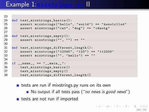
Example 1:mixstrings.py II
2324 def test_mixstrings_basics ():
25 assert mixstrings("hello", "world") == "hweolrllod"
26 assert mixstrings("cat", "dog") == "cdaotg"
2728 def test_mixstrings_empty ():
29 assert mixstrings("", "") == ""
3031 def test_mixstrings_different_length ():
32 assert mixstrings("12345", "123") == "112233"
33 assert mixstrings("", "hello") == ""
3435 if __name__ == "__main__":
36 test_mixstrings_basics ()
37 test_mixstrings_empty ()
38 test_mixstrings_different_length ()
tests are run if mixstrings.py runs on its own
No output if all tests pass (“no news is good news”)
tests are not run if imported
309 / 334

Example 2: mixstrings-pytest I
1 import pytest
23 def mixstrings(s1, s2):
4 """ Given two strings s1 and s2 , create and return a new
5 string that contains the letters from s1 and s2 mixed:
6 i.e. s[0] = s1[0], s[1] = s2[0], s[2] = s1[1],
7 s[3] = s2[1], s[4] = s1[2], ...
8 If one string is longer than the other , the extra
9 characters in the longer string are ignored.
1011 Example:
1213 In []: mixstrings (" Hello", "12345")
14 Out []: ’H1e2l3l4o5 ’
15 """
16 # what length to process
17 n = min(len(s1), len(s2))
18 # collect chars in this list
19 s = []
2021 for i in range(n):
22 s.append(s1[i])
310 / 334

Example 2: mixstrings-pytest II
23 s.append(s2[i])
24 return "".join(s)
2526 def test_mixstrings_basics ():
27 assert mixstrings("hello", "world") == "hweolrllod"
28 assert mixstrings("cat", "dog") == "cdaotg"
2930 def test_mixstrings_empty ():
31 assert mixstrings("", "") == ""
3233 def test_mixstrings_different_length ():
34 assert mixstrings("12345", "123") == "112233"
35 assert mixstrings("", "hello") == ""
3637 if __name__ == "__main__": # need filename
38 pytest.main("-v mixstrings -pytest.py") # to test here
pytest finds functions starting with test automatically
and executes them. Output when tests pass:
311 / 334
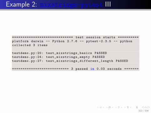
Example 2: mixstrings-pytest III
============================= test session starts ==========
platform darwin -- Python 2.7.6 -- pytest -2.3.5 -- python
collected 3 items
testdemo.py:20: test_mixstrings_basics PASSED
testdemo.py:24: test_mixstrings_empty PASSED
testdemo.py:27: test_mixstrings_different_length PASSED
=========================== 3 passed in 0.03 seconds =======
312 / 334
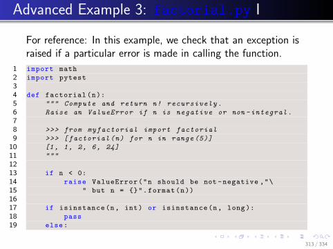
Advanced Example 3: factorial.py I
For reference: In this example, we check that an exception israised if a particular error is made in calling the function.
1 import math
2 import pytest
34 def factorial(n):
5 """ Compute and return n! recursively .
6 Raise an ValueError if n is negative or non -integral.
78 >>> from myfactorial import factorial
9 >>> [factorial(n) for n in range (5)]
10 [1, 1, 2, 6, 24]
11 """
1213 if n < 0:
14 raise ValueError("n should be not -negative ,"\
15 " but n = {}".format(n))
1617 if isinstance(n, int) or isinstance(n, long):
18 pass
19 else:
313 / 334

Advanced Example 3: factorial.py II
20 raise ValueError("n must be integer , or long ,"\
21 " but type(n)={}"\
22 .format(type(n)))
2324 # actual calculation
25 if n == 0:
26 return 1
27 else:
28 return n * factorial(n - 1)
2930 def test_basics ():
31 assert factorial (0) == 1
32 assert factorial (1) == 1
33 assert factorial (3) == 6
3435 def test_against_standard_lib ():
36 for i in range (20):
37 assert math.factorial(i) == factorial(i)
3839 def test_negative_number_raises_error ():
40 with pytest.raises(ValueError ): # this will pass if
41 factorial (-1) # factorial (-1) raises
42 # an ValueError
314 / 334

Advanced Example 3: factorial.py III
4344 def test_noninteger_number_raises_error ():
45 with pytest.raises(ValueError ):
46 factorial (0.5)
4748 if __name__ == "__main__":
49 pytest.main("-v factorial.py")
Output from successful testing:
============================= test session starts ==========
platform darwin -- Python 2.7.6 -- pytest -2.3.5 -- python
collected 4 items
factorial.py:28: test_basics PASSED
factorial.py:33: test_against_standard_lib PASSED
factorial.py:37: test_negative_number_raises_error PASSED
factorial.py:42: test_noninteger_number_raises_error PASSED
=========================== 4 passed in 0.02 seconds =======
315 / 334
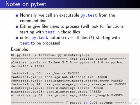
Notes on pytest
Normally, we call an executable py.test from thecommand lineEither give filenames to process (will look for functionsstarting with test in those filesor let py.test autodiscover all files (!) starting withtest to be processed.
Example:$> py.test -v factorial.py mixstrings.py
============================= test session starts =========
platform darwin -- Python 2.7.6 -- pytest -2.3.5 -- python
collected 7 items
factorial.py:30: test_basics PASSED
factorial.py:35: test_against_standard_lib PASSED
factorial.py:39: test_negative_number_raises_error PASSED
factorial.py:44: test_noninteger_number_raises_error PASSED
mixstrings.py:24: test_mixstrings_basics PASSED
mixstrings.py:28: test_mixstrings_empty PASSED
mixstrings.py:31: test_mixstrings_different_length PASSED
=========================== 7 passed in 0.04 seconds ====== 316 / 334

Testing summary
Testing know as Unit testing, regression testing, systemtesting
absolute key role in modern software engineering
good practice to always write tests when code is written
bigger projects have ”continuous integration testing”
”extreme programming” philosophy suggests to writetests before you write code
Executable py.test and python module pytest are not partof the standard python library.
317 / 334

Some Programming Languages
for Computational Science
see also: http://www.levenez.com/lang/
for an overview of general programming languages
318 / 334

Requirements
In the early days . . .
computers were slow and rare
computing time was very precious
invest effort to run programs as fast as possible
Nowadays . . .
increasingly more computing power available
major cost factor is the time it takes to write (and debugand test) software
This is not always true (because it depends on the application)but it seems to be generally correct.
319 / 334

Fortran
FORmula TRANslator (design goal is to translateformulae)
1957: Fortran I
commonly used:
Fortran 66 and 77Fortran 90 and 95(“matrix notation”)
compiled language, “low level”
inbuilt complex numbers → popular with scientists
very fast
many numerical libraries are written in Fortran
outlook: Fortran 2003 introduces “Objects”
320 / 334
C
developed 1972 in Bell laboratories
1978 Kerninghan & Ritchie C (often called K&R)
1989 ANSI C
design goals:
economy of expressionabsence of restriction
compiled language, “low level”
UNIX/Linux written in C
no inbuilt complex numbers
very fast
some numerical libraries are written in C
general purpose language (in comparision to Fortran)
321 / 334

C++
developed 1983 Bjarne Stroustrup
compiled language, “low level”
Object Oriented
set of higher-level tools (STL)
fast
C is subset of C++ but
knowing C does not mean knowing C++
general purpose language
322 / 334

MATLAB
MATrix LABoratory (1984)started as collection of linear algebra functionsscripting language grew to combine these functionsvisualisation features were addedthis is what we call MATLAB todaythe MATLAB scripting language is interpreted and slowthe numerical libraries that come with MATLAB arecompiled and fastdesigned for numerical work (and very good at this)can be fast if used carefully“high-level language” → higher coding efficiencycommercial product
need to payusers can not see source code
can not check code
very popular in engineering community323 / 334

Python
1990 Python (named after Monty Python)
high coding efficiency due to
“high-level language”interpretedsimple syntax and clean designhuge tool box, including GUIs, internet, XML, databases, graphics, gaming, numerical processing
general purpose language
easy to include compiled Fortran and C code
re-use of existing librariesway to make Python programs fast
fully supports Object Orientation
performance comparable to MATLAB
growing popularity in commerce, science and industry
324 / 334

Comparison
Selected criteria:
Fortran C C++ Matlab Pythonperformance + + + ◦ ◦
object orientation – – + – +exceptions – – + – +
open source + + + – +easy to learn ◦+ ◦ ◦– + +
legend:
+ = good/yes◦ = so-so– = poor/no
325 / 334

How do Python and MATLAB relate?
both MATLAB and Python share (good) ideas:
provide high-level scripting language (slow) to gluetogetherfast compiled libraries
Some differences are:
MATLAB is written for Engineering and ComputationalScience tasks and leading in combining computation andvisualisation.MATLAB is a commercial product.Python is a modern, general purposes language andeasier to extend.“Large” projects are better advised to use Python as theglueing language.
326 / 334
Summary
Need Fortran and C for extreme speed
Need high-level language to reduce development time(that is time for writing the program)
This is particularly important in a research environmentwhere requirements often change.
Strategy:
write parts of the code that take most of the executiontime in C/Fortranwrite the remaining program (for visualisation, datainput output, . . . ) in high-level language.For large computational programs, generally ¿ 99% ofthe CPU time are spend in a few % of the code.
327 / 334

The next steps . . .
328 / 334

What language to learn next?
. . . it all depends what you want to achieve:
To learn C or Fortran, get a book or on-line tutorial.
To learn object oriented programming (OOP), read “Howto think like a computer Scientist” (for Python), or try“Python – how to program” (see next slides).
To learn C++, learn OOP using Python first, then switchto C++.
To learn Java or C#, you should consider learning OOPusing Python first (but you could risk switching languagestraight away).
Note:
Python provides an excellent platform for all possible tasks
⇒ it could well be all you need for some time to come.
329 / 334

Further reading (1)
“How to Think Like aComputer Scientist: Learningwith Python”. (ISBN0971677506) free at
http://www.greenteapress.com/thinkpython/
Very systematic presentation ofall important programmingconcepts, including OOP.
Aimed at first year computerscience students.
Recommended if you likeprogramming and want toknow more about the concepts.
330 / 334

Further reading (2)
“Python How to Program”(ISBN 0130923613), ≈ £42
Very detailed presentation ofimportant programmingconcepts.
Many, many examples.
Includes chapters on XML,Graphical user interfaces,network programming, database interfacing and more.
Recommended if you like to dostuff with Python (for examplewriting a networked tic-tac toegame with GUI, . . . )
331 / 334

Further reading (3)
“Python Scripting forComputational Science” (ISBN3540435085), ≈ £40.
Excellent summary of use ofPython in ComputationalScience and Engineering.
Includes pointers to usefullibraries, visualisation utilities,good practice and integrationof compiled code.
Recommended if you need touse Python for scientificcomputation.
332 / 334

Other tools and topics
Tools to round of your computational toolkit / suggestedself-study topics
Systematic testing (py.test or nose)
Version control (try Mercurial or Git)
IPython Notebook
Latex (professional document creation)
Cool editor (Emacs? Sublime? ...)
333 / 334

changeset: 411:9e7fc455e6fb
tag: tip
parent: 391:2cfd852e8dc4
parent: 410:f1b1539dfb1a
334 / 334