pushing the tipping in international environmental agreements

Pushing the Tipping inInternational Environmental Agreements

Lorenzo Cerda Planas∗

WORKING PAPER

Last revision: December 29th, 2014

Abstract

This paper intends to provide an alternative approach to explain the formation ofInternational Environmental Agreements (IEA). The existing consensus from the lit-erature suggests that there are either too few signatories or that the emissions of signa-tories are almost the same as business as usual (BAU). I start from well known model(Barrett 1997), adding heterogeneity in countries’ marginal abatement costs (low andhigh) and in damages suffered (or corresponding environmental concern). I also allowfor technological transfers and border taxes. I show that using either mechanism oneat a time, does not change the results. But if both are used in a ’strategic’ manner, agrand (and abating) coalition can be reached, while minimizing transfers.

JEL Classification: F53, C63, C72, F18, Q58, O32.Keywords: Self-enforcing environmental agreements, border tax, tipping.

∗Paris School of Economics, C.E.S. - Université de Paris 1 Panthéon-Sorbonne; 106-112, Boulevard del’Hôpital, 75647 Paris Cedex 13, France. Email: [email protected]

1

1 Introduction

The present paper focuses on the idea that trying to have an International Environ-mental Agreement (IEA) that brings together a big share of countries into joining it, issometimes a colossal task to achieve. Barrett (1994) [2], Rubio & Ulph (2006) [15] andEichner & Pethig (2013) [11] among others, show that the number of signatories of self-enforcing IEAs does not exceed three or four. Recent failures on reaching an effectiveagreement concerning climate change is a clear example of this fact. Other solutions thathave been analysed in order to arrive to a successful IEA have to do with the idea of start-ing with a small sub-set of countries that can incorporate others as time goes by. This ideahas been already explored by Heal and Kunreuther (2011) [13], where they suggest a smallcoalition that adds countries to it, in a cascading process. Following this line Carraro &Siniscalco (1993) [7], Hoel & Schneider (1997) [14] and Barrett (2001) [4] have analysed theset-up in where transfers has been introduced in order to induce more countries to join theIEA. Unfortunately all these papers showed that a commitment problem prevent the for-mation of the grand coalition or if it forms, it almost acts as Business as Usual (BAU). Thecommitment problem comes from the fact that the IEA set-up resembles a chicken game.Therefore signatories are better off compared to not having an IEA at all, but they wouldprefer to actually have others to sign and themselves to be non-signatories. Hence, whentransfers are made in order to enlarge the coalition, the original signatories prefer to leave.

With all these barriers in mind, I explore a new tactic and I show that using two instru-ments, namely a border tax and technology transfers, it can effectively induce and sustainthe grand and meaningful coalition.(1) I also show that these transfers have to be madeto the least-green countries, in order to improve the chances of success, while minimizingthe amount of transfers.

In order to develop this idea, I will use as a baseline the model developed by Barrett(1997) [3], and then I will add some ingredients. The first one is the possibility of trans-fers between countries, as in Carraro and Siniscalco (1993) [7]. The second one has todo with the idea that societies behave green, even though direct ‘rational’ thinking couldcommand otherwise. This could be related to moral reasons rather than economic ones.As shown in Cerda (2013) [8], structurally similar countries (in development level, politi-cal system) can end up behaving differently with respect to the environment. This couldbe for historical reasons, but the point is that some countries became (quite) aware ofthe environmental problem at hand and started acting accordingly. This point supportsthe idea of having heterogeneity in countries, which departs from the two last cited pa-

(1)Meaningful in the sense that countries are actually doing an effort in abating and not behaving closeto BAU.

2

pers. In this paper, the differences among countries are how green they are, and whatabatement technology they have in place. With respect to the first point, an equivalentinterpretation can be on how countries are affected by pollution. Therefore having highermarginal damages coming from emission will be treated as a synonym of being greener.On the abatement side, countries can either have a costly technology (also referred as a’bad’ technology) and an cheap technology (the good one).

With this set-up I want to check if a small initial coalition of green countries can in-duce the formation of the grand coalition. The idea behind is the same as the successfulmechanism implemented in the Montreal protocol and its subsequent amendments (for adetailed explanation see Barrett’s book [5]). It this case one country, the US, was unilat-erally willing to cut emissions and consumption of ozone depleting substances. But theywere well aware that first, leakage coming from trade could reduce their effort results,and secondly that if other big economies would follow suit, the gains (for them and glob-ally) would be much better. Therefore they were willing to unilaterally ban the use andproduction of CFCs, but also to ban trade of these substances. This second component,plus the fact that they were also willing to help developing countries to switch to new andclean substances, pushed others countries to join one of the most successful IEA knownin history.

Therefore it would be desirable to do a similar thing with green house gases (GHG)emissions. But for this case some important barriers appear. First, tackling the productionand trade of CFCs is an simple task. Where doing the same for CO2 emissions is quiteimpossible, since their emissions are embedded in almost every product we trade. Hence,completely banning trade seems out of the question. The ’sticks’ used in Montreal are notcredible in an IEA concerning CO2. To avoid this obstacle, we can use a border tax, im-posed on goods coming from non-signatories countries, in order to deter free-riding andto induce accession, similarly as Montreal did with trade ban. This will be the case in thepresent paper, acknowledging that this could bring a trade war. In order to avoid this, Iwill use conservative values for this tax, in line with the results of Anouliès (2014) [1]. Apossible drawback of this upper limit is that the stick looses its deterring force and it isquite possible that this is the reason why such an agreement has not been put in place sofar.

A second point to note is the fact that in the CFC case, the estimated losses comingfrom high UV rays exposition and the costs of changing technology, made the choice aneasy one. The gains exceed the costs by a huge margin, making the political decisionviable. Returning to the CO2 problem, although there is a big consensus about dam-ages arising from global warming, there are differences among countries of how these

3

damages will hurt each one and moreover, the damage level is uncertain and eventuallycomparable to the cost of switching to the required clean technology. This factor is animportant one since even though in the Montreal case, a Minimum Participation Clause(MPC) was needed in order to induce the desired equilibrium (and not to suffer from free-riding if there were too few signatories). But there was consensus on the damages comingfrom not doing so. In the present conundrum, having uncertainty of gains and costs ofaccessing such an agreement, makes the political decision a much harder one to pursuit,and puts the MPC in a level that might not be politically feasible to reach. Or it has suchan uncertainty that it becomes political infeasible. Due to this last point I will assumethat in order to reach the grand coalition, no MPC should be needed. This premise mightseem to hard, but the idea behind it is that if the grand coalition can be reached with thisassumption, then it can be reached with a ’small’ MPC, which might be politically accept-able. Since this last point is hard to determine, I choose to rule out the use of a MPC.

With all these previous considerations in mind I build a model which is an expandedversion of Barrett (1997) [3]. To keep focus on the main objective of the paper, I use somebasic premises. I assume that it is profitable for that grand coalition to form, meaningthat the gains coming from cutting emissions are higher than the abatement cost andconsumption and production loss coming from mitigating them. I also assume that theparameters of the model are such that there exists an initial (small) coalition of greencountries.

2 The Game

There is always a trade-off between simplicity and reality when choosing the model.Therefore I start with a ’simple’ model, to which I add some features and at the same timeI will introduce some simplifications, in order to keep it tractable. To do so, I build on themodel used by Barrett (1997) [3]. This model is a three stage game where countries chooseto be part or not of an IEA (one shot), then governments set their abatement levels (whichtheir firms must meet) and then firms move by choosing simultaneously their segmentedoutputs, all this in a Cournot-Nash set-up. It is a perfect information model in the sensethat countries perfectly know their costs and gains and the same of other countries.

The idea of choosing this model is that it has some features that are useful to the taskat hand. First, it focusses on abatement technology and not in emissions. This is impor-tant since, from a ’political’ point of view, it leads to an enforceable IEA since technologybeing used is easily verifiable, where total emissions could be arguable. A second point,an most important to this work, is that I can add technology transfers (carrots), whichchanges the recipient country’s incentives, and therefore the game itself, which is part of

4

the overall plan. On the other hand, it is easy to add asymmetries to the model. In mycase, I add two asymmetries: marginal abatement costs (two levels) and heterogeneityin the marginal damage from emissions (environmental concern). Third, it models trade,and therefore carbon leakage, which is a feature (and challenge) that cannot be left aside.The main obstacle in reaching an meaningful IEA comes from having leakage, because itprovides countries strong incentives to free-ride. In fourth place, the original model hassanctions (sticks): it bans trade. In my case I will replace the trade ban with a border tax,which follows the same intuition. It is a tool to hinder leakage and it is a credible one.

With the previous specifications, I define two types of countries: those with cheap(good) abatement technology and high marginal damage from emissions, the ’rich’ coun-tries; and those with expensive (bad) abatement technology and lower environmentalconcern, the ’outsiders’. I will be using marginal damage from emissions and environ-mental concern as synonyms, since as it will be seen in the following equations, the higherthe damage coming from emissions, the higher are the incentives to a country to reduceemissions (locally and globally) and to join and IEA. In this line I will be also referring tocountries with higher environmental concern as ’greener’.

Finally, I set two moments or stages: the base case, which is the case where border taxor technology transfers are allowed, but not both at the same time. In this case, I willassume that the conditions (parameters) are such that we get the classical result that thereis a small coalition in place or if the grand coalition is a possible equilibrium of the game,is such that we need a MPC in order to induce this equilibrium. The second stage, AfterTax and Transfers, is the one where both instruments are in place. In this case I will showthat the grand coalition forms(2), with no MPC as a requirement.

2.1 The model

There are N countries and there are N firms (one per country) that produce an ho-mogeneous traded good and a transboundary pollution. The inverse demand in eachcountry is given by p(xi) = 1− xi, where xi is the consumption of the good in country i.Firm j’s costs are C(σj, xj, qj) = σj qj xj, where xj is total output by firm j, σj is its marginalabatement cost and qj ∈ {0, 1} is the abatement standard for firm j. Firm j takes qj asgiven. Transport costs are zero. Emissions by firm j are xj(1− qj). Therefore if abatementis maximal, emissions are zero. If no abatement is undertaken, emissions are equal tooutput.

(2)I assume that the parameters are such that the big coalition is an equilibrium (with or without the needof a MPC), after transferring technology to one or more countries.

5

Looking at σj, the abatement marginal cost for firm j, it could reflect the technologyused, to produce electricity for example, in country j. Therefore it could be thought asthe (accumulative) efforts undertaken by a country in order to be greener. In this modelthere are two possible levels of marginal abatement cost: cheap (good) technology σL andexpensive (bad) technology σH.

Secondly we have the stick: the border tax. In this case, instead of banning tradebetween signatories and non-signatories, I have that countries inside a coalition will taximports, at a rate t, of goods coming (and produced) from non-signatories countries. Inthis set-up I assume that only signatory tax goods coming from non-signatories and thatthe later do not retaliate with another tax on signatories’ goods. In order for this assump-tion to be credible (meaning that it does not trigger a trade war), I will use low tax ratelevels (although the model will be solved with a generic rate t), in line with Anouliès(2014) [1] results. The idea here is that the border tax will only reflect the cost that thenon-signatory country would have incurred if it had abated. In this sense, the maximumvalue of t will be the marginal abatement cost of the non-signatory, σH.

In third place country’s choice is binary: qj ∈ {0, 1}. Either the country chooses tofully abate (qj = 1) and none at all (qj = 0). Hence, joining the coalition and having qj = 1become synonyms. This change has two main basis: First, I discard by construction thecase of having coalitions (esp. the grand coalition) that do not abate or when they do,the operate quite close to BAU, as the literature has shown (as in Barrett (1994) [2] andEichner & Pethig (2013) [11]). Secondly, it makes the model more tractable with clear cutresults.(3) On another side, we can see that if country decisions are binary, it makes thecoalition formation a ’harder’ process, since becoming member of the IEA implies fullabatement for the joining country. Also signatories do not have any form to punish acountry leaving the coalition, since I assume a border tax rate constant and given. Hence,if a coalition can form in this stricter set-up, they would form in a laxer one.

Focussing now on the solution of the game at hand, I proceed using backward induc-tion. First I solve the firm production, which depends of the abatement undertaken byeach country. With this, each country j can evaluate two options, qj = 1 or qj = 0, whichalso depends of the decisions taken by others. With all this in mind, each country choosesto be part of the coalition of size k, Sk or not. Firms choose their output for each marketsimultaneously. Firm j takes its own abatement standard and the segmented outputs ofother firms as given and chooses a quantity to produce and ship to market i, xi

j, so as tomaximize,

πj =N

∑i=1

(1− xi − tij − σj qj)xi

j (2.1)

(3)Binary choices can also be found in the literature, as for example in Heal (1994) [12].

6

with tij = t if i ∈ Sk ∧ j /∈ Sk, and ti

j = 0 otherwise. First order conditions are(4)

1− xi − tij − σj qj − xi

j = 0 ∀i, j (2.2)

Taking into account the fact the qj ∈ {0, 1} and solving the system of equations, weget:

xi =

N−σS−(N−k)·t

N+1 if i ∈ Sk

N−σSN+1 if i /∈ Sk

(2.3)

where k is the size of the coalition, and σS = ∑j∈S σj (the sum of the coalition’s marginalabatement costs). Replacing this result into the FOC, we have:

xij =

1+σS−(N+1)σj+(N−k)·t

N+11+σS−(k+1)·t

N+1 if i ∈ Sk

1+σS−(N+1)σjN+1

1+σSN+1 if i /∈ Sk

(2.4)

↑ ↑if j ∈ Sk if j /∈ Sk

From where we can calculate the firm profit πj:(5)

πj =

N·ℵ2

j + k(N−k)t(

2ℵj+(N−k)t)

(N+1)2 if j ∈ Sk ℵj = 1 + σS − (N + 1)σj

N·ℵ22 + k(k+1)t

((k+1)t−2ℵ2

)(N+1)2 if j /∈ Sk ℵ2 = 1 + σS

with (2.5)

Countries choices

Country j’s net benefits are the sum of firm j’s profits, the consumer surplus of itscitizens, less the environmental damage suffered, plus border taxes collected, if it is thecase. Pollution is assumed to be a pure public bad and aggregate emissions are givenby ∑N

i=1 xi(1 − qi). Marginal environmental damage for each country is ωj. As statedin the Introduction, there is heterogeneity in ωj, with the rich countries having ωH and’outsiders’ having ωj < ωH (abusing the notation). For the consumer surplus we havethat, given demand specifications, it is equal to (xj)2/2 for country j. For the tax collected,we just add up those of the signatory countries (qj = 1) taxing products coming from thenon-signatories (qj = 0). With these, country profit is:

Πj = πj + (xj)2/2−ωj

[N

∑i=1

xi(1− qi)

]+ t · qj ·

N

∑i=1

xji(1− qi) (2.6)

(4)I only consider the situations where firms produce positive quantities in equilibrium.(5)Mathematical development of eqns. (2.2), (2.3) and (2.4) are in Appendix A.

7

where xj and xji are those found in equations (2.3) and (2.4) respectively, and xi is ∑N

j=1 xji ,

the production of firm i.

2.2 Enlarging the coalition

As stated in the Introduction, the idea is to show that starting from a Base Case mo-ment in where there is no grand coalition in place, we can arrive into a situation, calledAfter Tax and Transfers, where the grand and meaningful coalition forms. In order to arriveto this point, some r countries have to receive a technological transfer that reduces theirmarginal abatement cost from σH to σL. These technological transfers can be thought of aninternational aid from rich countries to some other countries in order to induce the grandcoalition formation. For example, rich countries could be willing to change how elec-tricity is produced, in order to shift from a carbon intensive power sources, into a moreeco-friendly ones. This transfer has a cost K per recipient and it is done only once. Theidea then is to minimize the amount r of recipient countries and to know to which coun-tries confer this new technology. It is also assumed that countries paying these transfersare the rich countries, which will be denoted by (σL, ωH), being them of an amount of d(for donors). In the same manner in the After Tax and Transfers stage we have r recipientsdenoted by (σL, ωj) and (N−d−r) non-recipients denoted by (σH, ωj).

In order to picture the game, I start with the Base Case where only d rich countries formpart of the coalition. This means that no other country is willing to join the coalition. Inparticular, we can see that to have this situation we only need that the greenest outsideris not willing to join. This is simply due to the fact that all outsiders share the same abate-ment technology σH and they only differ on their environmental concern ωj. Hence, if thegreenest one is not willing to join, from the country profit equation (2.6) is evident that noother will. It is important to note this, since having an heterogeneous set-up means that abroader amount of scenarios should be considered. Now, since countries that might jointhe coalition only differ on their environmental concern, I can order them from the green-est one to the least green one. I can now verify if this sequence (of all remaining countries)will be willing to join a given coalition. If it is not the case, we therefore know that thereis no other sequence that will make the job. It is worth noticing that this is a one-shotset-up, and therefore when I talk about a ’sequence’ of countries, implying therefore anorder, in reality what I am simulating is the thinking process of each country in order todecide if it will join or not a given coalition. In this sense and having in mind that a MPCis not allowed in this framework, we can understand the ’simultaneous’ decision processas following: Having a coalition in place of k countries, the greenest outsider evaluatesif it is profitable for it to join or not. Obviously all countries are doing this at the sametime, but let us imagine that for this country it is profitable, no matter what the rest do.

8

So it will be willing to join and other countries know this. Hence, it may be the case that’now’ it is also profitable for the second greenest country, no matter what the rest do (andit correctly assumes that it is so for the greenest). In this way, we could have a ’cascading’process ending up with all countries joining the coalition. Of course, when I talk of a’cascading’ I am not implying a dynamic process, but only this strategic reasoning thatcountries do, in order to decide their accession. In the same manner, we can clearly seethat if this ’ordered’ sequence of countries do not produced the full cascading (meaningto reach the grand coalition), therefore no other ’order’ will. Since all countries know this,they proceed accordingly.(6)

On the other hand, we can have two cases when referring to being profitable (or not):We can either assume that it is profitable for each one, individually and without profitsharing among the coalition, or we can assume countries belonging a coalition share theirprofits. The first case is straightforward, where in the second case we would have topay attention to the sharing rule. But I will have no need to rely on this since I will onlyanalyse if a given coalition or an evaluated coalition (when players are analysing differentscenarios) is Internally Stable (IS).(7) In other words, I only verify if the sum of profits of acoalition of k countries is greater than the sum of their outside options, meaning the profiteach country would get if it leaves the coalition and a coalition of the remaining (k−1)countries forms. In the following I will refer to the second case, but it will be clear thatproofs and the reasoning underlying them work for the first case too. The IS conditioncan be represented as

∑j∈Sk

Πsj > ∑

j∈Sk

Πooj (2.7)

where Πsj is the country profit of a signatory (belonging to the coalition of size k: Sk) and

Πooj is the country outside option (for the same group of countries). If inequality (2.7) is

divided by k (the coalition size), we can talk of the mean coalition profit and the meanoutside option, which will turn out to be more convenient.

Base case

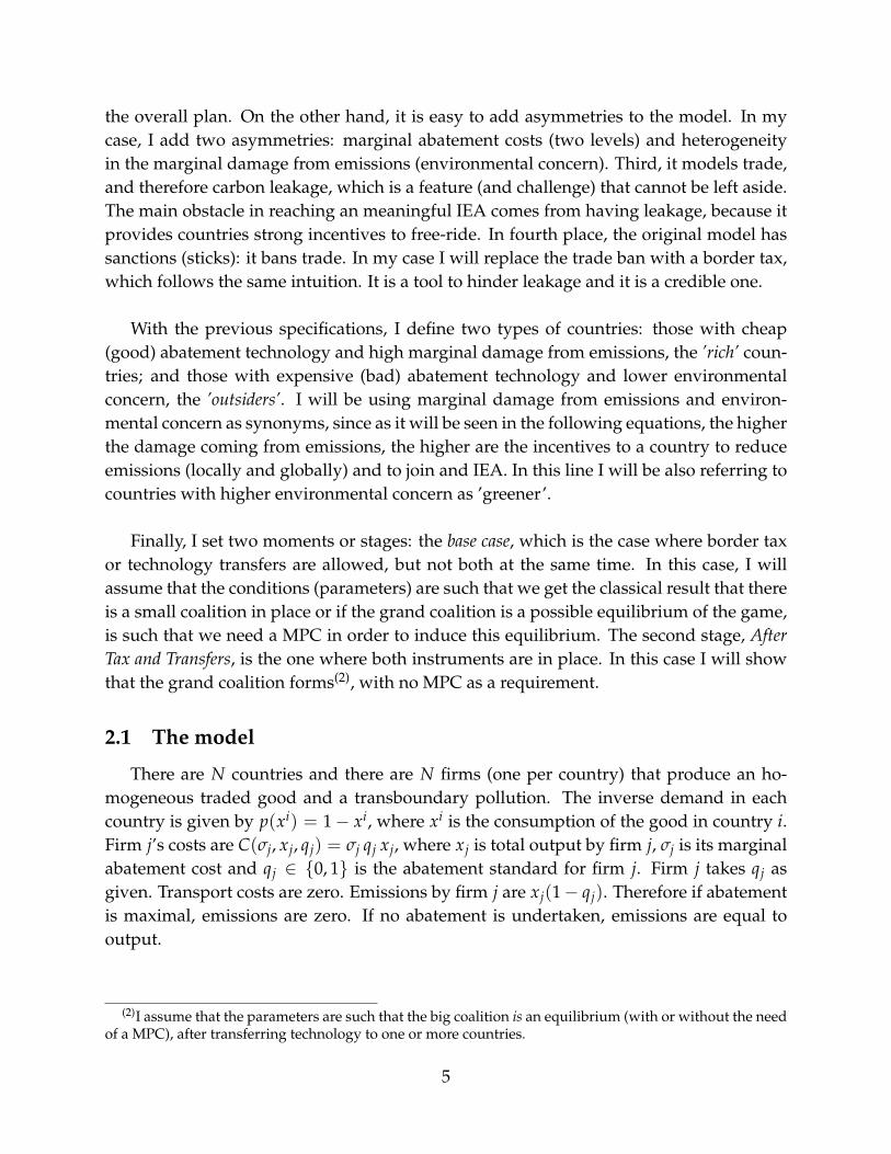
In order to give the intuition of the game at hand, I start simulating two cases of thebase case. To visualize the decision making process I will use the same type of graphicrepresentation as in Barrett (1997) [3], Carraro (1999) [6] and Diamantoudi & Sartzetakis(2006) [10]. Fig. 1a illustrates the case in where the border tax is implemented, but no

(6)It could also be considered a dynamic case where countries join sequentially. If this where the case,a discount factor for future gains or losses should be introduced and a timing system, which would addmore complexity to the model. Since the idea is to keep to model as simple as possible, I do not considerthis option, although the reader can visualise this scenario too.

(7)Internal and External Stability as defined by D’Aspremont et al. 1983 [9] and subsequently used by asubstantial literature.

9

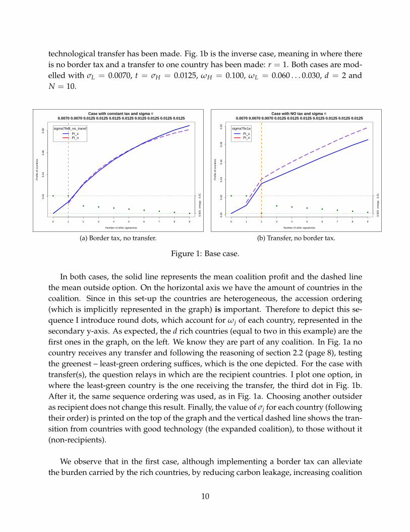
technological transfer has been made. Fig. 1b is the inverse case, meaning in where thereis no border tax and a transfer to one country has been made: r = 1. Both cases are mod-elled with σL = 0.0070, t = σH = 0.0125, ωH = 0.100, ωL = 0.060 . . . 0.030, d = 2 andN = 10.

● ●

●●

●●

●●

●●

0.00

30.

01om

ega

0.42

0.44

0.46

0.48

Number of other signatories

Pro

fits

of c

ount

ries

0 1 2 3 4 5 6 7 8 9

sigma79x8_no_transf

Pi_sPi_n

Case with constant tax and sigma = 0.0070 0.0070 0.0125 0.0125 0.0125 0.0125 0.0125 0.0125 0.0125 0.0125

(a) Border tax, no transfer.

● ●

●

●●

●●

●●

●

0.00

30.

01om

ega

0.40

0.42

0.44

0.46

0.48

0.50


Pro

fits

of c

ount

ries

0 1 2 3 4 5 6 7 8 9

sigma79x1a

Pi_sPi_n

Case with NO tax and sigma = 0.0070 0.0070 0.0070 0.0125 0.0125 0.0125 0.0125 0.0125 0.0125 0.0125

(b) Transfer, no border tax.

Figure 1: Base case.

In both cases, the solid line represents the mean coalition profit and the dashed linethe mean outside option. On the horizontal axis we have the amount of countries in thecoalition. Since in this set-up the countries are heterogeneous, the accession ordering(which is implicitly represented in the graph) is important. Therefore to depict this se-quence I introduce round dots, which account for ωj of each country, represented in thesecondary y-axis. As expected, the d rich countries (equal to two in this example) are thefirst ones in the graph, on the left. We know they are part of any coalition. In Fig. 1a nocountry receives any transfer and following the reasoning of section 2.2 (page 8), testingthe greenest – least-green ordering suffices, which is the one depicted. For the case withtransfer(s), the question relays in which are the recipient countries. I plot one option, inwhere the least-green country is the one receiving the transfer, the third dot in Fig. 1b.After it, the same sequence ordering was used, as in Fig. 1a. Choosing another outsideras recipient does not change this result. Finally, the value of σj for each country (followingtheir order) is printed on the top of the graph and the vertical dashed line shows the tran-sition from countries with good technology (the expanded coalition), to those without it(non-recipients).

We observe that in the first case, although implementing a border tax can alleviatethe burden carried by the rich countries, by reducing carbon leakage, increasing coalition

10

firms profits and getting and extra revenues (from taxes), it does not trigger the grandcoalition formation. On the other side, making only one technology transfer and not im-plementing a border tax is even worse. The absence of border tax makes the rich countriesmuch worse off and the transfer by itself does not induce the recipient country to join (andstay) in the coalition.

We can also note that in the first case, if MPC were possible (dismissed by assumption),a MPC of 6 countries could trigger the grand coalition formation. It is important to notethe goal of the instruments (border tax and transfers) is to reduce the MPC, up to thepoint in where there is no more need of it, meaning that the extended coalition (rich +recipients) can induce by itself the ’cascading’ process explained before.

After Tax and Transfers

Let us now study the case where a border tax has been implemented and transfers toone or more recipients have been made. The first question that arises is: which countriesare the recipients? I show that, if a group of r recipients produces the cascading (work-ing jointly with the border tax), then the set of groups that satisfies this condition alwaysincludes the group of outsiders that are the least-green. This result can appear counter in-tuitive at the beginning. We have to note two things: first, since countries are of the samesize, the cost to switch their abatement technology from σH to σL is always K, regardlessof how green the country is. Secondly, knowing that r countries are recipients, then Ihave (N−d−r) non-recipients. Therefore the goal is to make these (N−d−r) countriesto produce the cascading. Following a similar line of thought of section 2.2, leaving thegreenest countries in the non-recipients group is the best thing to do, since these are thecountries more prone to access any given coalition. Knowing that the expanded coalitioncountries have cheap technology, the ones expanding this coalition into the grand-coalitionwill be the ones that will bear the higher abatement costs.

To prove this, I will assume that there is a group r of recipients countries that producethe whole cascading. Abusing a little with the notation, r will refer either to the amountof recipient countries and/or the group of such countries. I show then that if a new recip-ient group r′ is formed, changing one country of the original r group with one less-greencountry from the non-recipients, then (d+r′) also produces the cascading. Iterating inthe modification of the recipient group, I arrive to (d+r∗), where r∗ is the group of theleast-green outsiders (of the same size of r), which again generates the cascading.

Let us call Cascading 1 the case where it is supposed that the expanded coalition (d+r)produces the cascading. This means that for each i non-recipient that enters the coali-tion (in a greenest – less-green ’order’ as stated before), we have that the IS condition in

11

(2.7) holds. In the same manner, let us denote Cascading 2 the case where we have sub-stituted one country of the r group with one country from the non-recipients, which isless-green than the replaced one, naming this new recipient group as r′. I show that thenew expanded coalition (d + r′) also produces the cascading, hence:

Proposition 2.1 Within the game set-up described above and with d being the amount of initialrich countries in the coalition, r a recipient group (of r countries) that produces the whole cascading(Cascading 1) for all i between 1 and N−d−r, then the whole cascading is also produced startingfrom the coalition (d + r′), where r′ is a less-green recipient group of r countries (Cascading 2):

Πd+r+is > Πd+r+i−1

n︸︷︷︸Cascading 1

⇒ ′Πd+r+is > ′Πd+r+i−1

n︸︷︷︸Cascading 2

∀i ∈ {1, . . . , N−d−r} (2.8)

where Πd+r+is is the non-recipient profit in a coalition of members (d+r+i) (d donors,

r recipients and i non-recipients). The prime in ′Π indicates that we are in Cascading2, meaning that the recipient group is r′ and that the sequence i of non-recipients com-ing into the coalition has been replaced accordingly. The following diagram shows the isequence for Cascadings 1 and 2:

1 2 m-1 m p p+1 N-d-r..… ..… ..…

1 2 m-1 m p-1 p+1 N-d-r..… ..… ..…

Phase.1 Phase.2 Phase.3

p-1

p'

Casc.1

Casc.2

(greenest) (least-green)

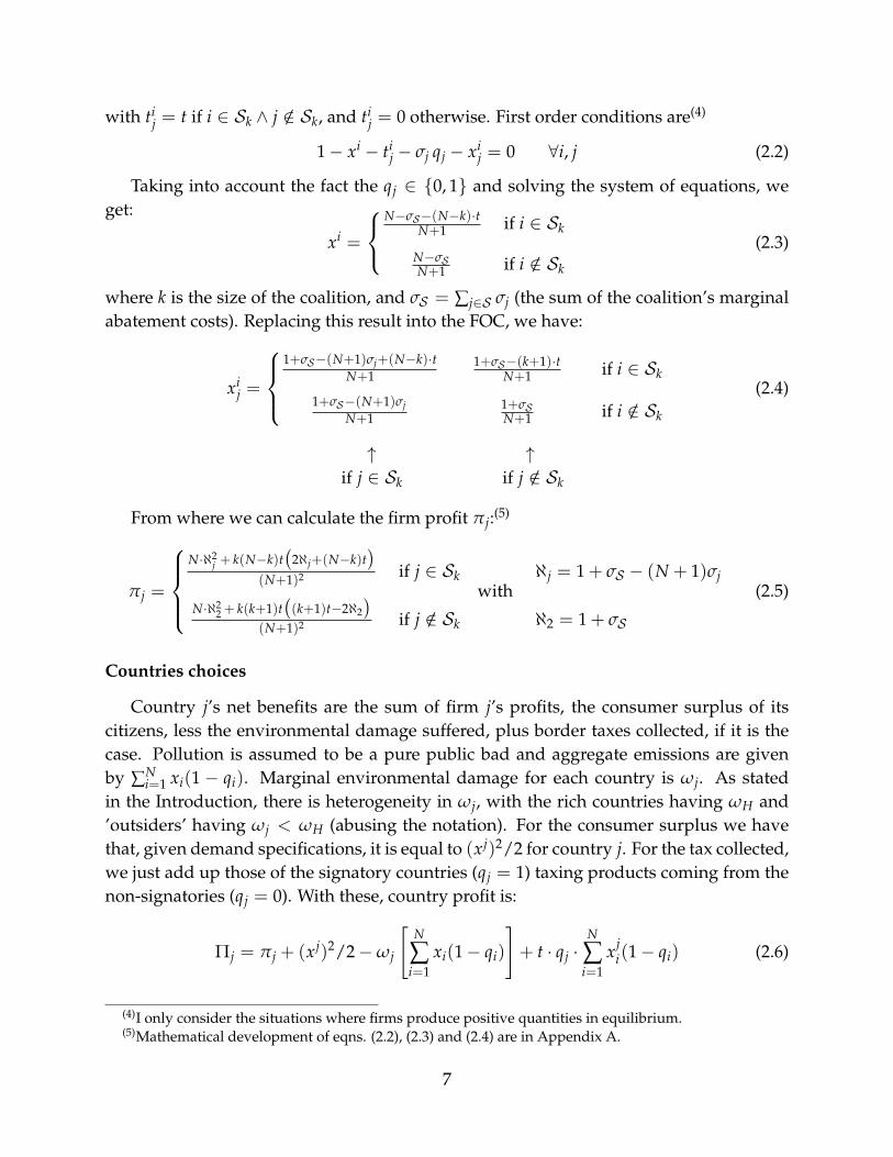
Figure 2: Non-recipients sequence for Cascadings 1 and 2.

As it can be noted in Fig. 2, the non-recipient sequence has been divided in 3 phases.This comes from the fact that as we have replaced one country in r, namely [p], whichhas entered into r′, replacing the country [p′] which now is in the non-recipient sequence.Due to this, the sequence has been modified, where phases 1 and 3 are unchanged andthe modification only applies to the countries in phase 2. By construction [p′] is greenerthan [p] and therefore enters before in the cascading process, as shown in the previousfigure.

12

The proof consist on showing that for each phase, the following two inequalities (In-equality 1 and 2) hold and therefore proving 2.8:

Cascading 1︷︸︸︷′Πd+r+i

s ≥ Πd+r+is︸︷︷︸

Inequality 1

> Πd+r+i−1n ≥ ′Πd+r+i−1

n︸︷︷︸Inequality 2︸︷︷︸

Cascading 2(2.9)

A detailed proof can be found in Appendix B. This result states that the set of recipi-ent groups that can produce the cascading always contains the group of the r least greencountries of outsiders. This is because in some cases, depending on the parameters cho-sen, this set can contain only one group, r∗, or more than one, but always including r∗.Therefore, if the rich countries want to make a technology transfer in order to induce thegrand coalition, they know where to start. The question now is to find out how many arethese r∗ countries.

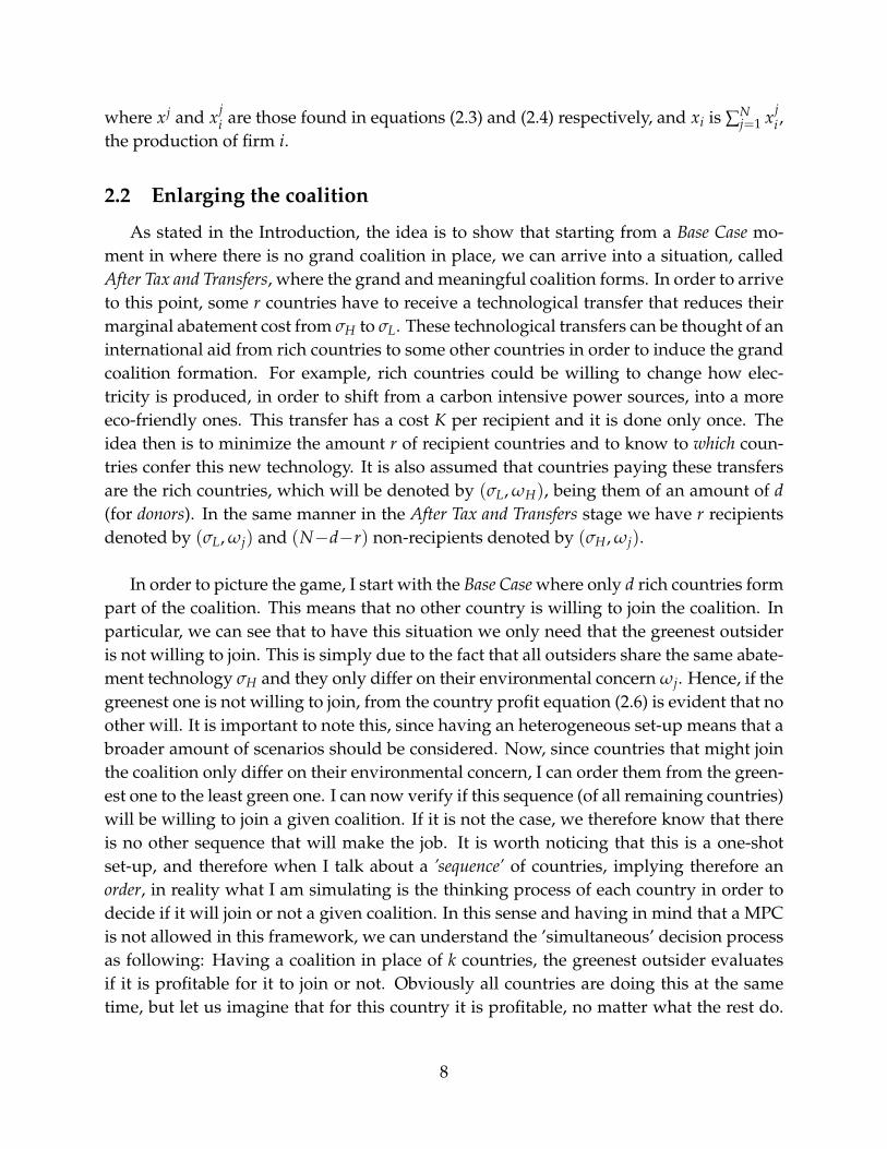
Before answering the previous question, let us observe an example of a transfer thatproduces a cascading in the following figure. I have used the same parameters as ofthe previous examples and the cascading has been triggered with only one recipient:r∗ = 1. The intuition is as follows: the technology transfer ’buys in’ the least-green coun-try, putting it inside the expanded coalition and changing its incentive for abating, sincenow it is cheaper for it. By doing so, we have ’artificially’ enlarged the initial coalitionwhere now the border tax helps to sustain it. This was the same occurring in the exam-ple depicted in Fig. 1a. The difference now is that the cascading has started with (d+r)countries (instead of only d). Therefore when the ’revenue’ effect, coming from the bordertax diminishes, as countries join the coalition, the IS conditions keep holding. After somemore countries have joint the coalition, the border tax has a ’punitive’ effect, in the sensethat now, non-signatories exports are facing a ’disadvantage’ with respect to the rest ofthe world. Now, after the revenue effect has diminished and before the punitive effect hascome into place, there is critical period where the IS condition might not hold, as it hap-pened before. It is like this cascading process mimics a mountain crossing(8) (in this casepeaking around k = 3 or 4), where the outside option is the mountain to be crossed andthe mean coalition profit is the maximum altitude we reach reach at each step. With onlythe border tax, the domino effect stops at some point: the mountain could not be crossed.But combining the border tax and a transfer (when leaving out the greenest countries)allows us to make it through. Both instruments reinforce themselves and it is not simplythe sum of them.

(8)As in the Mountain Crossing theorem.

13

● ●

●

●●

●●

●●

●

0.00

30.

01om

ega

0.42

0.44

0.46

0.48


Pro

fits

of c

ount

ries

0 1 2 3 4 5 6 7 8 9

sigma79x1a

Pi_sPi_n

Case with constant tax and sigma = 0.0070 0.0070 0.0070 0.0125 0.0125 0.0125 0.0125 0.0125 0.0125 0.0125

With transfer, and with tax

Transfer to theleast green one

’Punitive’effect

Revenue effect

Figure 3: After Tax and Transfers.

2.3 Finding the amount of recipients r∗

Let us resume with the question of how many r∗ recipients we need in order to pro-duce the full cascading. Unfortunately, equations get extremely complex in order to geta readable solution for this question, as they develop from the IS condition (inequality(2.7)). Therefore, when we plug in the country profits, which are composed of firm prof-its, consumer surpluses, environmental damages and tax revenues, the algebra just getsout of hand. In any case, these equations are provided in Appendix B. As a second ap-proach, I relied on simulations in order to show how r∗ would go. To do so, I definea ∆Πs

oo(d, r, i) function, which is just inequality (2.7) with all terms put on the left side.Therefore, if for a given value of r, ∆Πs

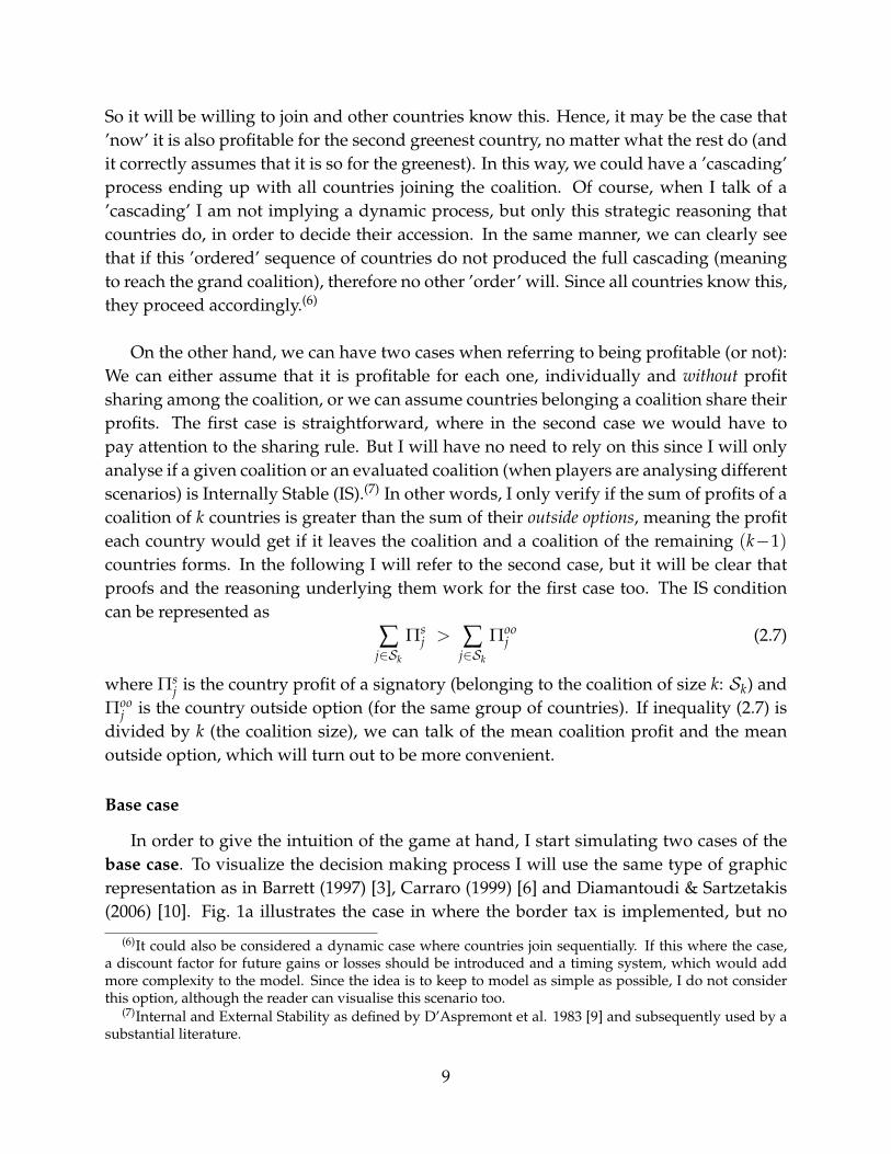
oo(d, r, i) > 0 for all possible i’s (d is given), then weget the full cascading. It is worth noting that I can build this function since I know whichcountries I have to ’buy in’ at each r level. In Fig. 4 we can observe a continuous versionof this function(9) for the same parameters used in the previous examples.

(9)This is coming directly from the country profit function. The only ’trick’ used was that I had to create acontinuous version of ∑ ωj to be used in the damage part of this function. The domain of ∆Πs

oo is restrictedto octant I (+++) and with (d+r+i) ≤ N, which is the area of interest.

14

0

0 1 2 3 4

0

0.002

0.004

0.006

0.008

0

01

23

45

67

8

r = amount of recipients

i = a

mou

nt o

f non

−re

cipi

ents

Case: All − Sum of deltas of donors, recipients and non−recipients.omega = 0.0100, 0.0100, 0.0080, 0.0074, 0.0069, 0.0063, 0.0057, 0.0051, 0.0046, 0.0040

d = 2 sigma_l = 0.0070 sigma_h = 0.0125

∆Πsoo(d, r, i) > 0

∆Πsoo(d, r, i) = 0

d+r+i ≤ 10

Figure 4: Contour of function ∆Πsoo(d, r, i), with d = 2.

The figure shows the solution area where ∆Πsoo(d, r, i) > 0, and more importantly, its limit

∆Πsoo(d, r, i) = 0. Therefore it is easy to see that the solution for this case is r∗ = 1. With

r = 0 we have the Base Case where there is no transfer and border tax is implemented.Following the vertical dashed line at r = 0, we can observe that we have the same resultas before. For values of i between 0 and 0.8 and then from 3.2 until the end, the value of∆Πs

oo > 0. In the range left in between, it is negative, meaning that for this case we arein need of a MPC, if we want to reach the grand coalition (we are not able to cross themountain). In the case with r = 1, we can clearly see that ∆Πs

oo > 0 for all the range of i,meaning that full cascading occurs. Following this reasoning, r∗ can be found by checkingwhen ∂r/∂i = 0 in the implicit function between r and i, given by ∆Πs

oo = 0. Hence wefind a maximum (of r with respect to i in this implicit function) and r∗ is just the integergreater or equal to this maximum. This development can also be found in Appendix B(Work in Progress).

A handy feature of this graphical representation is that it allows us to analyse what

15

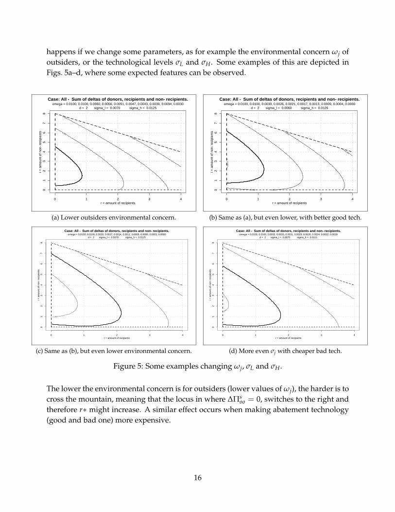
happens if we change some parameters, as for example the environmental concern ωj ofoutsiders, or the technological levels σL and σH. Some examples of this are depicted inFigs. 5a–d, where some expected features can be observed.

0

0 1 2 3 4

0

0.002

0.004

0.006

0

01

23

45

67

8


i = a

mou

nt o

f non

−re

cipi

ents


d = 2 sigma_l = 0.0070 sigma_h = 0.0125

(a) Lower outsiders environmental concern.

0

0 1 2 3 4

−0.002

0

0.002 0.002

0.004

0.006

0

01

23

45

67

8


i = a

mou

nt o

f non

−re

cipi

ents


d = 2 sigma_l = 0.0060 sigma_h = 0.0125

(b) Same as (a), but even lower, with better good tech.

0

0 1 2 3 4

−0.002

0

0.002

0.004

0 01

23

45

67

8


i = a

mou

nt o

f non

−re

cipi

ents


d = 2 sigma_l = 0.0070 sigma_h = 0.0125

(c) Same as (b), but even lower environmental concern.

0

0 1 2 3 4

−0.002

0

0.002

0.004

0 01

23

45

67

8


i = a

mou

nt o

f non

−re

cipi

ents


d = 2 sigma_l = 0.0070 sigma_h = 0.0111

(d) More even σj with cheaper bad tech.

Figure 5: Some examples changing ωj, σL and σH.

The lower the environmental concern is for outsiders (lower values of ωj), the harder is tocross the mountain, meaning that the locus in where ∆Πs

oo = 0, switches to the right andtherefore r∗ might increase. A similar effect occurs when making abatement technology(good and bad one) more expensive.

16

Paying transfers

One question that has been left aside is if these r transfers are worth while. The as-sumption is that rich countries pay for these transfers and therefore the logical questionis if they are actually willing to do so. They will if their gains coming from switchingfrom a small equilibrium of d countries into the grand coalition of N countries are biggerthan the transfers cost (K · r) divided among themselves, d. Noting that when all countriesabate there are no damages coming from emissions and neither taxes are being levied, thecomparison simplifies a bit into de gain/loss in firm profits and consumer surplus, plusthe forgone damages and less the taxes, which have disappeared. Denoting a subscriptd for rich countries and superscripts N and d for the grand coalition and initial coalitionrespectively, it is profitable if the following inequality holds:

(πNd − πd

d)︸︷︷︸>0

+ (CSNd − CSd

d)︸︷︷︸<0

−Damdd︸︷︷︸

>0

−Taxesdd︸︷︷︸

<0

≥ K · rd

(2.10)

Again the algebra gets nasty and detailed results can be found in Appendix C. Twoextreme cases can be easily analysed though: if K = 0 rich countries can always producethe cascading. Actually, they can just buy-in all outsiders (which induce the grand coali-tion by assumption). Moreover, the LHS of inequality (2.10) is positive too, since if it werenot the case, it would not be any (serious) environmental issue even to start with. On theother side, if K is just too big, then it is obvious that transfers might never be profitable.On the other hand, the LHS of this inequality imposes a ceiling to r, meaning that for agiven value of K, even if there exists a r∗ that produces the cascading, it might be too highin order for the rich countries to finance these transfers. Moreover, the LHS contains r,(10)

which makes the algebraic solution not attractive.

(10)This is due to the fact that firm profits and CS for donors are influenced by the total abatement technol-ogy used in the world, at the grand coalition case. Hence the term r · (σH − σL) appears having a negativeimpact in firm profits and a positive one in CS.

17

3 Conclusions

The present work explores a different approach for reaching an International Environ-mental Agreement (IEA). Following Heal and Kunreuther’s (2011) [13] idea, that a set ofcountries could tip the rest from a dirty equilibrium to a clean one, I have developed asimple model that shows that this is possible. Starting from a well-known model (Barrett(1997) [3]) and adding some heterogeneity in countries and simplifying in other features,I have shown that a small group of countries (for example, 2 out of 10) can actually inducethis cascading process. The first stage of this process ’buys-in’ some countries to the ini-tial coalition. But after having these countries on board, they could impose costs to non-joiners, costs such as border taxes, in order to finalize the cascading process, somethingsimilar to what happened with the Montreal Protocol and its subsequent amendments. Inthis later case, trade bans were possible due to the nature of the pollutant (specificity ofCFCs), where in the present conundrum (CO2 emissions and climate change) this instru-ment is not a credible threat.

An interesting result is that in order to minimize transfers and to improve the chancesof reaching the grand coalition, the recipient countries are those with least environmentalmarginal damage, also referred as the least-green ones. Although it might be a coinci-dence, it looks like this is what is happening with the bilateral agreement between theU.S. and China, reached this last November. Of course in this case, other considerationsare at hand, as size and emissions of the two specific countries. Another point to note isthe reinforcement effect between the border tax and a technological transfer. The bordertax by itself is not sufficient to induce the grand coalition, since it need some critical massto work. On the other hand, the transfer by itself does not work alone either, since it doesnot deal with the free-rider incentives. But both used, and in a proper way, have a lever-age effect among them, making the grand coalition a feasible outcome.

Finally and in order to expand this work, two options can be thought of. The firstone is the direct application of these two tools, the border tax and the transfers, in a morerealistic set-up and using real data. For example, a model with 6 or 12 regions could beused in order to test the feasibility of the solution proposed here. A second vein couldbe to analyse the strategic interplay in being a recipient or not. This comes from thefact that non-recipients do not receive any incentive (since they will accede due to thetrade pressure). Therefore, this might induce them to join the agreement in an earlierstage, and hence getting the transfer. This strategic interplay can again be anticipated bythe promoters of the IEA and by the rest of the players, enlarging the game set-up andeventually changing or reasserting the previous result.

18

References[1] Lisa Anouliés. The strategic and effective dimensions of the border tax adjustment. Journal

of Public Economic Theory, pages n/a–n/a, 2014.

[2] Scott Barrett. Self-enforcing international environmental agreements. Oxford Economic Papers,46:pp. 878–894, 1994.

[3] Scott Barrett. The strategy of trade sanctions in international environmental agreements.Resource and Energy Economics, 19(4):345–361, November 1997.

[4] Scott Barrett. International cooperation for sale. European Economic Review, 45(10):1835–1850,December 2001.

[5] Scott Barrett. Environment and Statecraft: The Strategy of Environmental Treaty-Making: TheStrategy of Environmental Treaty-Making. Oxford University Press, 2003.

[6] Carlo Carraro. The structure of international environmental agreements. In Carlo Carraro,editor, International Environmental Agreements on Climate Change, volume 13 of Fondazione EniEnrico Mattei (Feem) Series on Economics, Energy and Environment, pages 9–25. Springer Nether-lands, 1999.

[7] Carlo Carraro and Domenico Siniscalco. Strategies for the international protection of theenvironment. Journal of Public Economics, 52(3):309–328, October 1993.

[8] Lorenzo Cerda Planas. Moving to greener societies: Moral motivation and green behaviour.Working paper, Paris School of Economics - Université Paris 1 Panthéon - Sorbonne, August2014.

[9] Claude D’Aspremont, Alexis Jacquemin, Jean Jaskold Gabszewicz, and John A. Weymark.On the stability of collusive price leadership. The Canadian Journal of Economics / Revue cana-dienne d’Economique, 16(1):pp. 17–25, 1983.

[10] Effrosyni Diamantoudi and Eftichios S Sartzetakis. Stable international environmental agree-ments: An analytical approach. Journal of public economic theory, 8(2):247–263, 2006.

[11] Thomas Eichner and Rüdiger Pethig. Self-enforcing environmental agreements and interna-tional trade. Journal of Public Economics, 102(0):37 – 50, 2013.

[12] Geoffrey Heal. Formation of international environmental agreements. In Carlo Carraro,editor, Trade, Innovation, Environment, volume 2 of Fondazione Eni Enrico Mattei (FEEM) Serieson Economics, Energy and Environment, pages 301–322. Springer Netherlands, 1994.

[13] Geoffrey Heal and Howard Kunreuther. Tipping climate negotiations. Technical report, Na-tional Bureau of Economic Research, 2011.

[14] Michael Hoel and Kerstin Schneider. Incentives to participate in an international environ-mental agreement. Environmental and Resource Economics, 9(2):153–170, 1997.

[15] SJ Rubio and A Ulph. Self-enforcing agreements and international trade in greenhouse emis-sion rights. Oxford Economic Papers, 58:233–263, 2006.

19

A Firm maximization problem

The firm’s profit function to be maximized is the following:

πj =N

∑i=1

(1− xi − tij − σj qj)xi

j (A.1)

with tij = t if i ∈ Sk ∧ j /∈ Sk, and ti

j = 0 otherwise. I only consider situations where firmsproduce positive quantities in equilibrium. We can get the first order conditions, whichare:

1− xi − tij − σj qj − xi

j = 0 ∀i, j (A.2)

Summing over i, conditions in equations A.2 can be rewritten as:

N(1− σj qj)− 2xj − x−j − tj = 0 ∀j (A.3)

where tj = ∑Ni=1 ti

j is the sum of the tax rates ’paid’ by product produced by country j,

xj = ∑Ni=1 xi

j is the total output of firm j, and x−j = ∑k 6=j xik is the rest-of-the-world output.

This can be re-written in a matrix form, getting:2 1 · · · 11 2 · · · 1...

... . . . ...1 1 · · · 2

x1

x2...

xN

=

N − Nσ1 q1

N − Nσ2 q2...

N − NσN qN

−

t1

t2...

tN

(A.4)

︸︷︷︸C · −→xj = D

Using the Sherman-Morrison formula, we can get −→xj = C−1 · D, being

C−1 = I − BN + 1

where I is the identity matrix and B (of dimension N by N) is a matrix of ones. This givesthe general solution of:

−→xj =1

N + 1

N −1 · · · −1−1 N · · · −1

...... . . . ...

−1 −1 · · · N

N − Nσ1 q1 − t1

N − Nσ2 q2 − t2...

N − NσN qN − tN

Or equivalently:

xj =1

N + 1

[N(

1− Nσjqj − tj + ∑i 6=j

σiqi

)+ ∑

i 6=jti

](A.5)

20

Finally, for the country consumption levels xi, we can use the FOC (eqn. A.2) and weget:

xi =N −∑N

j=1 σj qj − ti

N + 1(A.6)

with ti = ∑Nj=1 ti

j being the sum of tax rates imposed by country i. Given that only signato-ries tax non-signatories products, we have that:

ti =

(N−k) · t if i ∈ Sk

0 if i /∈ Sk

which yields to

xi =

N−σS−(N−k)·t

N+1 if i ∈ Sk

N−σSN+1 if i /∈ Sk

(A.7)

where σS = ∑j∈S σj (the sum of the coalition’s marginal abatement costs). Replacingthis result into the FOC (Eqn. (A.2)), we finally have the segmented production of firm jshipped to country i:

xij =

1+σS−(N+1)σj+(N−k)·t

N+11+σS−(k+1)·t

N+1 if i ∈ Sk

1+σS−(N+1)σjN+1

1+σSN+1 if i /∈ Sk

(A.8)

↑ ↑if j ∈ Sk if j /∈ Sk

Finally, having xj, xi and xij and recalling the equations for the firm profit (πj), con-

sumer surplus (CSj), environmental damage (DAMj) and taxes collected (TAXj), we get:

πj =

N·ℵ2

j + k(N−k)t(

2ℵj+(N−k)t)

(N+1)2 if j ∈ Sk ℵj = 1 + σS − (N + 1)σj

N·ℵ22 + k(k+1)t

((k+1)t−2ℵ2

)(N+1)2 if j /∈ Sk ℵ2 = 1 + σS

with (A.9)

CSj =

(

N−σS−(N−k)t)

2(N+1)2 if j ∈ Sk(N−σS

)2(N+1)2 if j /∈ Sk

(A.10)

DAMj = −ωj ·(N − k)N + 1

·((1 + σS)N − k(k + 1)t

)(A.11)

TAXj = t · (N − k) ·

(1 + σS − (k + 1)t

)N + 1

(A.12)

21

B Proof of r∗ being the least-green recipient group

As stated in subsection 2.2, the proof consists in showing that if conditions for Cas-cading 1 hold, then conditions for Cascading 2 hold too. In order to do so, I will use tofollowing inequalities:

Cascading 1︷︸︸︷′Πd+r+i

s ≥ Πd+r+is︸︷︷︸

Inequality 1

> Πd+r+i−1n ≥ ′Πd+r+i−1

n︸︷︷︸Inequality 2︸︷︷︸

Cascading 2(B.1)

Hence, the proof resumes to showing that Inequality 1 and Inequality 2 hold. The first onesays that the profit of an ith country coming into the coalition ′Πd+r+i

s (Cascading 2) isgreater or equal than the same profit in the case of Cascading 1, where r′ has been replacedby the original r and the ith country entering the coalition might or might not be the sameof Cascading 2, according to the following diagram:

1 2 m-1 m p p+1 N-d-r..… ..… ..…

1 2 m-1 m p-1 p+1 N-d-r..… ..… ..…

Phase.1 Phase.2 Phase.3

p-1

p'

Casc.1

Casc.2

(greenest) (least-green)

Figure 6: Non-recipients sequence for cascadings 1 and 2.

The same has to be done for Inequality 2, where now we have to show that the outsideoption of an ith country coming into the coalition Πd+r+i−1

n (Cascading 1) is greater orequal than its counterpart in Cascading 2. To do so, I will analyse the possible changes infirm profits, consumer surplus, damages and taxes collected. As shown in the previouspicture I will divide the analysis in three phases: 1, 2 and 3.

First, let us note that the amount σS = ∑j∈S σj (the sum of the coalition’s marginalabatement costs) does not change between Cascading 1 and 2. In this due to the simplefact that the group of countries with good technology is always of size (d+ r). In the sameway, ℵj and ℵ2 stay constant between those two cases. Therefore the only difference that

22

may arise comes from the replacement of ωj, either of countries accessing the coalition(the i’s) or those in the recipient group (r or r′).

Inspecting the firm profit equation (A.9) it is clear that its value does not change be-tween Cascading 1 and 2. The same holds for the consumer surplus and for the taxescollected. Hence we only have to focus on the damages coming from emissions. Study-ing this equation shows as that emissions are also invariant between these two cases, sincethey only depend on σS and k. Hence the only changes comes directly from the term −ωj(in Eqn. (A.11)).

Define ∆D1 =′ DAMd+r+ij −DAMd+r+i

j , which is the difference in damages of countryj between Cascading 2 and 1 cases, in the presence of a coalition of size (d+r+i). In thesame manner, define ∆D2 =′ DAMd+r+i−1

j −DAMd+r+i−1j , which is just the same, with

a coalition of size (d+r+i−1). Finally, denote ωp the corresponding marginal damagefor the country p in r being replaced by a less-green country q in r′. And let ωq be themarginal damage of the replacing country q.

Let us start with the signatories (Inequality 1). In phase 1, ∆D1 = (ωp−ωq) · emissions,which is positive. In phase 2 we will have a similar case, where the pair of ω’s at stakewill be: ωp v/s ωm, ωm v/s ωm+1 . . . ωm+j−1 v/s ωm+j (recall Fig. 6) and thereforeresulting again in ∆D1 > 0. For phase 3, since the coming countries i’s and the groupalready in the coalition (d+r+i−1) have the same ω’s, ∆D1 = 0. Therefore, for phases 1,2 and 3 together we have that: ∆D1 ≥ 0 which proves Inequality 1.

For the case of non-signatories (Inequality 2) we have that for phases 1 and 3, ∆D2 = 0,since here we are only concerned on the entering country. For these two phases, the en-tering country is the same for both Cascadings. Following the same reasoning of phase 2in the previous paragraph, we get that ∆D2 < 0 for this phase. Putting the three phasestogether leads to ∆D2 ≤ 0, which again proves Inequality 2 (note that Inequality 2 has theCascading 1 and 2 inverted with respect to Inequality 1).

This last point proves that Cascading 1 implies Cascading 2. We iterate on the swap-ping process in r′, until the recipient group becomes r∗ the least-green outsider, whichfinishes the proof.

C Profitability of transfers for rich countriesTranscription in progress. Please visit my page at www.parisschoolofeconomics.

eu/en/cerda-planas-lorenzo/ or send me a request by email (see cover page) foran updated version.

23

pushing the tipping in international environmental agreements

Documents