pure metric geometry: introductory lectures
TRANSCRIPT
arX
iv:2
007.
0984
6v4
[m
ath.
MG
] 2
0 Se
p 20
21
Pure metric geometry:
introductory lectures
Anton Petrunin

We discuss only domestic affairs of metric spaces; applications aregiven only as illustrations.
These notes could be used as an introductory part to virtually anycourse in metric geometry. It is based on a part of the course in metricgeometry given at Penn State, Spring 2020. The complete lecturescan be found on the author’s website; it includes an introduction toAlexandrov geometry based on [1] and metric geometry on manifolds[28] based on a simplified proof of Gromov’s systolic inequality givenby Alexander Nabutovsky [22].
A part of the text is a compilation from [1, 2, 24, 26, 27] and itsdrafts.
I want to thank Sergio Zamora Barrera for help.
Contents
1 Definitions 5
A Metric spaces . . . . . . . . . . . . . . . . . . . . . . . . 5
B Variations of definition . . . . . . . . . . . . . . . . . . . 6
C Completeness . . . . . . . . . . . . . . . . . . . . . . . . 7
D Compact spaces . . . . . . . . . . . . . . . . . . . . . . . 8
E Proper spaces . . . . . . . . . . . . . . . . . . . . . . . . 9
F Geodesics . . . . . . . . . . . . . . . . . . . . . . . . . . 9
G Geodesic spaces and metric trees . . . . . . . . . . . . . 9
H Length . . . . . . . . . . . . . . . . . . . . . . . . . . . . 10
I Length spaces . . . . . . . . . . . . . . . . . . . . . . . . 11
2 Universal spaces 15
A Embedding in a normed space . . . . . . . . . . . . . . . 15
B Extension property . . . . . . . . . . . . . . . . . . . . . 17
C Universality . . . . . . . . . . . . . . . . . . . . . . . . . 19
D Uniqueness and homogeneity . . . . . . . . . . . . . . . 20
E Remarks . . . . . . . . . . . . . . . . . . . . . . . . . . . 22
3 Injective spaces 23
A Admissible and extremal functions . . . . . . . . . . . . 23
B Injective spaces . . . . . . . . . . . . . . . . . . . . . . . 25
C Space of extremal functions . . . . . . . . . . . . . . . . 27
D Injective envelope . . . . . . . . . . . . . . . . . . . . . . 29
E Remarks . . . . . . . . . . . . . . . . . . . . . . . . . . . 30
4 Space of sets 31
A Hausdorff distance . . . . . . . . . . . . . . . . . . . . . 31
B Hausdorff convergence . . . . . . . . . . . . . . . . . . . 32
C An application . . . . . . . . . . . . . . . . . . . . . . . 34
D Remarks . . . . . . . . . . . . . . . . . . . . . . . . . . . 35
3
5 Space of spaces 37
A Gromov–Hausdorff metric . . . . . . . . . . . . . . . . . 37B Approximations . . . . . . . . . . . . . . . . . . . . . . . 39C Almost isometries . . . . . . . . . . . . . . . . . . . . . . 39D Convergence . . . . . . . . . . . . . . . . . . . . . . . . . 41E Uniformly totally bonded families . . . . . . . . . . . . . 42F Gromov’s selection theorem . . . . . . . . . . . . . . . . 43G Universal ambient space . . . . . . . . . . . . . . . . . . 45H Remarks . . . . . . . . . . . . . . . . . . . . . . . . . . . 46
6 Ultralimits 49
A Faces of ultrafilters . . . . . . . . . . . . . . . . . . . . . 49B Ultralimits of points . . . . . . . . . . . . . . . . . . . . 50C Ultralimits of spaces . . . . . . . . . . . . . . . . . . . . 52D Ultrapower . . . . . . . . . . . . . . . . . . . . . . . . . 53E Tangent and asymptotic spaces . . . . . . . . . . . . . . 54F Remarks . . . . . . . . . . . . . . . . . . . . . . . . . . . 55
A Semisolutions 57
Bibliography 79
Lecture 1
Definitions
In this lecture we give some conventions used further and remind somedefinitions related to metric spaces.
We assume some prior knowledge of metric spaces. For a moredetailed introduction, we recommend the first couple of chapters inthe book by Dmitri Burago, Yuri Burago, and Sergei Ivanov [7].
A Metric spaces
The distance between two points x and y in a metric space X will bedenoted by |x− y| or |x− y|X . The latter notation is used if we needto emphasize that the distance is taken in the space X .
Let us recall the definition of metric.
1.1. Definition. A metric on a set X is a real-valued function (x, y) 7→7→ |x − y|X that satisfies the following conditions for any three pointsx, y, z ∈ X :
(a) |x− y|X > 0,
(b) |x− y|X = 0 ⇐⇒ x = y,
(c) |x− y|X = |y − x|X ,
(d) |x− y|X + |y − z|X > |x− z|X .
Recall that a metric space is a set with a metric on it. The elementsof the set are called points. Most of the time we keep the same notationfor the metric space and its underlying set.
The function
distx : y 7→ |x− y|
is called the distance function from x.
5
6 LECTURE 1. DEFINITIONS
Given R ∈ [0,∞] and x ∈ X , the sets
B(x,R) = y ∈ X | |x− y| < R,B[x,R] = y ∈ X | |x− y| 6 R
are called, respectively, the open and the closed balls of radius R withcenter x. If we need to emphasize that these balls are taken in themetric space X , we write
B(x,R)X and B[x,R]X .
1.2. Exercise. Show that
|p− q|X + |x− y|X 6 |p− x|X + |p− y|X + |q − x|X + |q − y|X
for any four points p, q, x, and y in a metric space X .
B Variations of definition
Pseudometris. A metric for which the distance between two distinctpoints can be zero is called a pseudometric. In other words, to definepseudometric, we need to remove condition (b) from 1.1.
The following observation shows that nearly any question aboutpseudometric spaces can be reduced to a question about genuine metricspaces.
Assume X is a pseudometric space. Consider an equivalence rela-tion ∼ on X defined by
x ∼ y ⇐⇒ |x− y| = 0.
Note that if x ∼ x′, then |y−x| = |y−x′| for any y ∈ X . Thus, |∗−∗|defines a metric on the quotient set X/∼. This way we obtain a metricspace X ′. The space X ′ is called the corresponding metric space forthe pseudometric space X . Often we do not distinguish between X ′
and X .
∞-metrics. One may also consider metrics with values in R ∪ ∞;we might call them ∞-metrics, but most of the time we use the termmetric.
Again nearly any question about ∞-metric spaces can be reducedto a question about genuine metric spaces.
Setx ≈ y ⇐⇒ |x− y| < ∞;
C. COMPLETENESS 7
it defines another equivalence relation on X . The equivalence class ofa point x ∈ X will be called the metric component of x; it will bedenoted by Xx. One could think of Xx as B(x,∞)X — the open ballcentered at x and radius ∞ in X .
It follows that any ∞-metric space is a disjoint union of genuinemetric spaces — the metric components of the original ∞-metric space.
1.3. Exercise. Given two sets A and B on the plane, set
|A−B| = µ(AB),
where µ denotes the Lebesgue measure and denotes symmetric dif-ference
AB := (A ∪B) \ (B ∩ A).
(a) Show that |∗ − ∗| is a pseudometric on the set of bounded closedsubsets.
(b) Show that |∗ − ∗| is an ∞-metric on the set of all open subsets.
C Completeness
A metric space X is called complete if every Cauchy sequence of pointsin X converges in X .
1.4. Exercise. Suppose that ρ is a positive continuous function on acomplete metric space X and ε > 0. Show that there is a point x ∈ Xsuch that
ρ(x) < (1 + ε)·ρ(y)for any point y ∈ B(x, ρ(x)).
Most of the time we will assume that a metric space is complete.The following construction produces a complete metric space X forany given metric space X .
Completion. Given a metric space X , consider the set C of all Cauchysequences in X . Note that for any two Cauchy sequences (xn) and (yn)the right-hand side in ➊ is defined; moreover, it defines a pseudometricon C
➊ |(xn)− (yn)|C := limn→∞
|xn − yn|X .
The corresponding metric space X is called completion of X .Note that the original space X forms a dense subset in its com-
pletion X . More precisely, for each point x ∈ X one can consider aconstant sequence xn = x which is Cauchy. It defines a natural map
8 LECTURE 1. DEFINITIONS
X → X . It is easy to check that this map is distance-preserving. Inparticular, we can (and will) consider X as a subset of X .
1.5. Exercise. Show that the completion of a metric space is com-plete.
D Compact spaces
Let us recall few equivalent definitions of compact metric spaces.
1.6. Definition. A metric space K is compact if and only if one ofthe following equivalent conditions hold:(a) Every open cover of K has a finite subcover.(b) For any open cover of K there is ε > 0 such that any ε-ball
in K lies in one element of the cover. (The value ε is called aLebesgue number of the covering.)
(c) Every sequence of points in K has a subsequence that convergesin K.
(d) The space K is complete and totally bounded; that is, for anyε > 0, the space K admits a finite cover by open ε-balls.
A subset N of a metric space K is called ε-net if any point x ∈ Klies on the distance less than ε from a point in N . Note that totallybounded spaces can be defined as spaces that admit a finite ε-net forany ε > 0.
1.7. Exercise. Show that a space K is totally bounded if and only ifit contains a compact ε-net for any ε > 0.
Let packε X be the exact upper bound on the number of pointsx1, . . . , xn ∈ X such that |xi − xj | > ε if i 6= j.
If n = packε X < ∞, then the collection of points x1, . . . , xn iscalled a maximal ε-packing. Note that n is the maximal number ofopen disjoint ε
2 -balls in X .
1.8. Exercise. Show that any maximal ε-packing is an ε-net.Conclude that a complete space X is compact if and only if packε X <
< ∞ for any ε > 0.
1.9. Exercise. Let K be a compact metric space and
f : K → Kbe a distance-nondecreasing map. Prove that f is an isometry; that is,f is a distance-preserving bijection.
A metric space X is called locally compact if any point in X admitsa compact neighborhood; in other words, for any point x ∈ X a closedball B[x, r] is compact for some r > 0.
E. PROPER SPACES 9
E Proper spaces
A metric space X is called proper if all closed bounded sets in Xare compact. This condition is equivalent to each of the followingstatements:
⋄ For some (and therefore any) point p ∈ X and any R < ∞, theclosed ball B[p,R]X is compact.
⋄ The function distp : X → R is proper for some (and thereforeany) point p ∈ X ; that is, for any compact set K ⊂ R, itsinverse image
dist−1p (K) = x ∈ X : |p− x|X ∈ K
is compact.
1.10. Exercise. Give an example of space which is locally compactbut not proper.
F Geodesics
Let X be a metric space and I a real interval. A globally isometricmap γ : I → X is called a geodesic1; in other words, γ : I → X is ageodesic if
|γ(s)− γ(t)|X = |s− t|for any pair s, t ∈ I.
If γ : [a, b] → X is a geodesic and p = γ(a), q = γ(b), then we saythat γ is a geodesic from p to q. In this case, the image of γ is denotedby [pq], and, with abuse of notations, we also call it a geodesic. Wemay write [pq]X to emphasize that the geodesic [pq] is in the space X .
In general, a geodesic from p to q need not exist and if it exists, itneed not be unique. However, once we write [pq] we assume that wehave chosen such geodesic.
A geodesic path is a geodesic with constant-speed parameterizationby the unit interval [0, 1].
G Geodesic spaces and metric trees
A metric space is called geodesic if any pair of its points can be joinedby a geodesic.
1Different authors call it differently: shortest path, minimizing geodesic. Also,note that the meaning of the term geodesic is different from what is used in Rie-mannian geometry, altho they are closely related.
10 LECTURE 1. DEFINITIONS
1.11. Exercise. Let f be a centrally symmetric positive continuousfunction on S2. Given two points x, y ∈ S2, set
‖x− y‖ =w
B(x,π2)\B(y,π
2)
f.
Show that (S2, ‖∗ − ∗‖) is a geodesic space and the geodesics in(S2, ‖∗ − ∗‖) run along great circles of S2.
A geodesic space T is called a metric tree if any pair of pointsin T are connected by a unique geodesic, and the union of any twogeodesics [xy]T , and [yz]T contain the geodesic [xz]T . In other wordsany triangle in T is a tripod; that is, for any three geodesics [xy], [yz],and [zx] have a common point.
1.12. Exercise. Let p, x, y, z be points in a metric tree. Considerthree numbers
a = |p− x|+ |y − z|, b = |p− y|+ |z − x|, c = |p− z|+ |x− y|.
Suppose that a 6 b 6 c. Show that b = c.
Recall that the set
Sr(p)X = x ∈ X : |p− x|X = r
is called a sphere with center p and radius r in a metric space X .
1.13. Exercise. Show that spheres in metric trees are ultrametricspaces. That is,
|x− z| 6 max |x− y|, |y − z|
for any x, y, z ∈ Sr(p)T .
H Length
A curve is defined as a continuous map from a real interval I to ametric space. If I = [0, 1], that is, if the interval is unit, then the curveis called a path.
1.14. Definition. Let X be a metric space and α : I → X be a curve.We define the length of α as
lengthα := supt06t16...6tn
∑
i
|α(ti)− α(ti−1)|.
A curve α is called rectifiable if lengthα < ∞.
I. LENGTH SPACES 11
1.15. Theorem. Length is a lower semi-continuous with respect tothe pointwise convergence of curves.
More precisely, assume that a sequence of curves γn : I → X in ametric space X converges pointwise to a curve γ∞ : I → X ; that is, forany fixed t ∈ I, γn(t) → γ∞(t) as n → ∞. Then
➊ limn→∞
length γn > length γ∞.
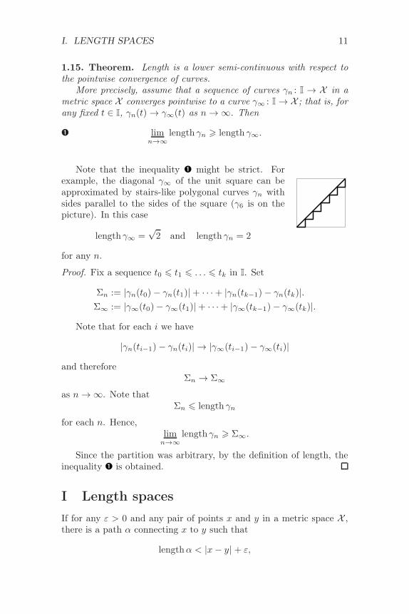
Note that the inequality ➊ might be strict. Forexample, the diagonal γ∞ of the unit square can beapproximated by stairs-like polygonal curves γn withsides parallel to the sides of the square (γ6 is on thepicture). In this case
length γ∞ =√2 and length γn = 2
for any n.
Proof. Fix a sequence t0 6 t1 6 . . . 6 tk in I. Set
Σn := |γn(t0)− γn(t1)|+ · · ·+ |γn(tk−1)− γn(tk)|.Σ∞ := |γ∞(t0)− γ∞(t1)|+ · · ·+ |γ∞(tk−1)− γ∞(tk)|.
Note that for each i we have
|γn(ti−1)− γn(ti)| → |γ∞(ti−1)− γ∞(ti)|
and thereforeΣn → Σ∞
as n → ∞. Note thatΣn 6 length γn
for each n. Hence,limn→∞
length γn > Σ∞.
Since the partition was arbitrary, by the definition of length, theinequality ➊ is obtained.
I Length spaces
If for any ε > 0 and any pair of points x and y in a metric space X ,there is a path α connecting x to y such that
lengthα < |x− y| + ε,
12 LECTURE 1. DEFINITIONS
then X is called a length space and the metric on X is called a lengthmetric.
An ∞-metric space is a length space if each of its metric compo-nents is a length space. In other words, if X is an ∞-metric space,then in the above definition we assume in addition that |x− y|X < ∞.
Note that any geodesic space is a length space. The followingexample shows that the converse does not hold.
1.16. Example. Suppose a space X is obtained by gluing a countablecollection of disjoint intervals In of length 1 + 1
n, where for each In
the left end is glued to p and the right end to q.Observe that the space X carries a natural complete length metric
with respect to which |p− q|X = 1 but there is no geodesic connectingp to q.
1.17. Exercise. Give an example of a complete length space X suchthat no pair of distinct points in X can be joined by a geodesic.
Directly from the definition, it follows that if α : [0, 1] → X is apath from x to y (that is, α(0) = x and α(1) = y), then
lengthα > |x− y|.Set
‖x− y‖ = inflengthαwhere the greatest lower bound is taken for all paths from x to y.It is straightforward to check that (x, y) 7→ ‖x − y‖ is an ∞-metric;moreover, (X , ‖∗ − ∗‖) is a length space. The metric ‖∗ − ∗‖ is calledthe induced length metric.
1.18. Exercise. Let X be a complete length space. Show that for anycompact subset K in X there is a compact path-connected subset K ′
that contains K.
1.19. Exercise. Suppose (X , |∗−∗|) is a complete metric space. Showthat (X , ‖∗ − ∗‖) is complete.
Let A be a subset of a metric space X . Given two points x, y ∈ A,consider the value
|x− y|A = infαlengthα,
where the greatest lower bound is taken for all paths α from x to yin A. In other words |∗ − ∗|A denotes the induced length metric onthe subspace A.2
2The notation |∗−∗|A
conflicts with the previously defined notation for distance|x−y|
Xin a metric space X . However, most of the time we will work with ambient
length spaces where the meaning will be unambiguous.
I. LENGTH SPACES 13
Let x and y be points in a metric space X .(i) A point z ∈ X is called a midpoint between x and y if
|x− z| = |y − z| = 12 ·|x− y|.
(ii) Assume ε > 0. A point z ∈ X is called an ε-midpoint between xand y if
|x− z|, |y − z| 6 12 ·|x− y| + ε.
Note that a 0-midpoint is the same as a midpoint.
1.20. Lemma. Let X be a complete metric space.(a) Assume that for any pair of points x, y ∈ X , and any ε > 0,
there is an ε-midpoint z. Then X is a length space.(b) Assume that for any pair of points x, y ∈ X , there is a mid-
point z. Then X is a geodesic space.
Proof. We first prove (a). Let x, y ∈ X be a pair of points.Set εn = ε
4n , α(0) = x and α(1) = y.Let α(12 ) be an ε1-midpoint between α(0) and α(1). Further, let
α(14 ) and α(34 ) be ε2-midpoints between the pairs (α(0), α(12 )) and(α(12 ), α(1)) respectively. Applying the above procedure recursively,
on the n-th step we define α( k2n ), for every odd integer k such that
0 < k2n < 1, as an εn-midpoint of the already defined α(k−1
2n ) and
α(k+12n ).In this way we define α(t) for t ∈ W , where W denotes the set
of dyadic rationals in [0, 1]. Since X is complete, the map α can beextended continuously to [0, 1]. Moreover,
➊lengthα 6 |x− y| +
∞∑
n=1
2n−1 ·εn 6
6 |x− y| + ε2 .
Since ε > 0 is arbitrary, we get (a).To prove (b), one should repeat the same argument taking mid-
points instead of εn-midpoints. In this case, ➊ holds for εn = ε == 0.
Since in a compact space a sequence of 1n-midpoints zn contains a
convergent subsequence, 1.20 immediately implies the following.
1.21. Proposition. Any proper length space is geodesic.
1.22. Hopf–Rinow theorem. Any complete, locally compact lengthspace is proper.
14 LECTURE 1. DEFINITIONS
Before reading the proof, it is instructive to solve 1.10.
Proof. Let X be a locally compact length space. Given x ∈ X , denoteby ρ(x) the least upper bound of all R > 0 such that the closed ballB[x,R] is compact. Since X is locally compact,
➋ ρ(x) > 0 for any x ∈ X .
It is sufficient to show that ρ(x) = ∞ for some (and therefore any)point x ∈ X .
➌ If ρ(x) < ∞, then B = B[x, ρ(x)] is compact.
Indeed, X is a length space; therefore for any ε > 0, the setB[x, ρ(x) − ε] is a compact ε-net in B. Since B is closed and hencecomplete, it must be compact.
➍ |ρ(x)− ρ(y)| 6 |x− y|X for any x, y ∈ X ; in particular, ρ : X → R
is a continuous function.
Indeed, assume the contrary; that is, ρ(x) + |x − y| < ρ(y) forsome x, y ∈ X . Then B[x, ρ(x) + ε] is a closed subset of B[y, ρ(y)] forsome ε > 0. Then compactness of B[y, ρ(y)] implies compactness ofB[x, ρ(x) + ε], a contradiction.
Set ε = min ρ(y) : y ∈ B ; the minimum is defined since B iscompact and ρ is continuous. From ➋, we have ε > 0.
Choose a finite ε10 -net a1, a2, . . . , an in B = B[x, ρ(x)]. The union
W of the closed balls B[ai, ε] is compact. Clearly, B[x, ρ(x)+ ε10 ] ⊂ W .
Therefore, B[x, ρ(x) + ε10 ] is compact, a contradiction.
1.23. Exercise. Construct a geodesic space X that is locally compact,but whose completion X is neither geodesic nor locally compact.
1.24. Advanced exercise. Show that for any compact length-metricspace X there is a number ℓ such that for any finite collection of pointsthere is a point z that lies on average distance ℓ from the collection;that is, for any x1, . . . , xn ∈ X there is z ∈ X such that
1n·∑
i
|xi − z|X = ℓ.
Lecture 2
Universal spaces
This lecture is based on the discussion of Urysohn space in the bookof Mikhael Gromov [12].
A Embedding in a normed space
Recall that a function v 7→ |v| on a vector space V is called norm ifit satisfies the following condition for any two vectors v, w ∈ V and ascalar α:
⋄ |v| > 0;
⋄ |α·v| = |α|·|v|;⋄ |v|+ |w| > |v + w|.As an example, consider the space of real sequences equipped with
sup norm denoted by the ℓ∞; that is, ℓ∞-norm of a = a1, a2, . . . isdefined by
|a|ℓ∞ = supn |an| .
It is straightforward to check that for any normed space the func-tion (v, w) 7→ |v − w| defines a metric on it. Therefore, any normedspace is an example of metric space (in fact, it is a geodesic space). Of-ten we do not distinguish between normed space and the correspondingmetric space.1
The following lemma implies that any compact metric space isisometric to a subset of a fixed normed space.
Recall that diameter of a metric space X (briefly diamX ) is definedas least upper bound on the distances between pairs of its points; that
1By Mazur–Ulam theorem, the metric remembers the linear structure of thespace; a slick proof of this statement was given by Jussi Vaisala [32].
15
16 LECTURE 2. UNIVERSAL SPACES
is,diamX = sup |x− y|X : x, y ∈ X .
2.1. Lemma. Suppose X is a bounded separable metric space; thatis, diamX is finite and X contains a countable, dense set wn. Givenx ∈ X , set an(x) = |wn − x|X . Then
ι : x 7→ (a1(x), a2(x), . . . )
defines a distance-preserving embedding ι : X → ℓ∞.
Proof. By the triangle inequality
➊ |an(x)− an(y)| 6 |x− y|X .
Therefore, ι is short (in other words, ι is distance non-increasing).Again by triangle inequality we have
|an(x)− an(y)| > |x− y|X − 2·|wn − x|X .
Since the set wn is dense, we can choose wn arbitrarily close to x.Whence the value |an(x) − an(y)| can be chosen arbitrarily close to|x− y|X . In other words
supn ||wn − x|X − |wn − y|X | > |x− y|X .
Hence
➋ supn |an(x) − an(y)| > |x− y|X ;
that is, ι is distance non-contracting.Finally, observe that ➊ and ➋ imply the lemma.
2.2. Exercise. Show that any compact metric space K is isometricto a subspace of a compact geodesic space.
The following exercise generalizes the lemma to arbitrary separablespaces.
2.3. Exercise. Suppose wn is a countable, dense set in a metricspace X . Choose x0 ∈ X ; given x ∈ X , set
an(x) = |wn − x|X − |wn − x0|X .
Show that ι : x 7→ (a1(x), a2(x), . . . ) defines a distance-preserving em-bedding ι : X → ℓ∞.
B. EXTENSION PROPERTY 17
The following lemma implies that any metric space is isometric toa subset of a normed vector space; its proof is nearly identical to theproof of 2.3.
2.4. Lemma. Let X be arbitrary metric space. Denote by ℓ∞(X ) thespace of all bounded functions on X equipped with sup-norm.
Then for any point x0 ∈ X , the map ι : X → ℓ∞(X ) defined by
ι : x 7→ (distx − distx0)
is distance-preserving.
B Extension property
If a metric space X is a subspace of a pseudometric space X ′, then wesay that X ′ is an extension of X . If in addition diamX ′ 6 d, then wesay that X ′ is a d-extension.
If the complement X ′\X contains a single point, say p, we say thatX ′ is a one-point extension of X . In this case, to define metric onX ′, it is sufficient to specify the distance function from p; that is, afunction f : X → R defined by
f(x) = |p− x|X ′ .
Any function f of that type will be called extension function or d-extension function respectively.
The extension function f cannot be taken arbitrary — the triangleinequality implies that
f(x) + f(y) > |x− y|X > |f(x)− f(y)|
for any x, y ∈ X . In particular, f is a non-negative 1-Lipschitz functionon X . For a d-extension, we need to assume in addition that diamX 6
6 d and f(x) 6 d for any x ∈ X . These conditions are necessary andsufficient.
2.5. Definition. A metric space U meets the extension property iffor any finite subspace F ⊂ U and any extension function f : F → R
there is a point p ∈ U such that |p− x| = f(x) for any x ∈ F .If we assume in addition that diamU 6 d and instead of extension
functions we consider only d-extension functions, then we arrive at adefinition of d-extension property.
If in addition U is separable and complete, then it is called Urysohnspace or d-Urysohn space respectively.
18 LECTURE 2. UNIVERSAL SPACES
2.6. Proposition. There is a separable metric space with the (d-)extension property (for any d > 0).
Proof. Choose d > 0. Let us construct a separable metric space withthe d-extension property.
Let X be a compact metric space such that diamX 6 d. Denoteby X d the space of all d-extension functions on X equipped with themetric defined by the sup-norm. Note that the map X → X d definedby x 7→ distx is a distance-preserving embedding, so we can (and will)treat X as a subspace of X d, or, equivalently, X d is an extension of X .
Let us iterate this construction. Start with a one-point space X0
and consider a sequence of spaces (Xn) defined by Xn+1 = X dn . Note
that the sequence is nested; that is, X0 ⊂ X1 ⊂ . . . and the union
X∞ =⋃
n
Xn;
comes with metric such that |x− y|X∞
= |x− y|Xnif x, y ∈ Xn.
Note that if X is compact, then so is X d. It follows that each spaceXn is compact. In particular, X∞ is a countable union of compactspaces; therefore X∞ is separable.
Any finite subspace F of X∞ lies in some Xn for n < ∞. Byconstruction, there is a point p ∈ Xn+1 that meets the condition in 2.5for any extension function f : F → R. That is, X∞ has the d-extensionproperty.
The construction of a separable metric space with the extensionproperty requires only minor changes. First, the sequence should bedefined by Xn+1 = X dn
n , where dn is an increasing sequence such thatdn → ∞. Second, the point p should be taken in Xn+k for sufficientlylarge k, so that dn+k > maxf(x).
2.7. Proposition. If a metric space V meets the (d-) extension prop-erty, then so does its completion.
Proof. Let us assume V meets the extension property. We will showthat its completion U meets the extension property as well. The d-extension case can be proved along the same lines.
Note that V is a dense subset in a complete space U . Observe thatU has the approximate extension property; that is, if F ⊂ U is a finiteset, ε > 0, and f : F → R is an extension function, then there existsp ∈ U such that
➊ |p− x| <> f(x)± ε
C. UNIVERSALITY 19
for any x ∈ F . Indeed, let us extend f to the whole X by setting
f(z) = inf f(x) + |x− z| : x ∈ F .
Observe that f is an extension function. Since V is dense in U , we canchoose a finite set F ′ ∈ V such that for any x ∈ F there is x′ ∈ F ′
with |x− x′| < ε2 . It remains to observe that the point p provided by
the extension property for the restriction f |F ′ meets ➊.Therefore, there is a sequence of points pn ∈ U such that for any
x ∈ F ,|pn − x| <> f(x) ± 1
2n .
Moreover, we can assume that
➋ |pn − pn+1| < 12n
for all large n. Indeed, consider the sets Fn = F ∪ pn and thefunctions fn : Fn → R defined by fn(x) = f(x) if x 6= pn and
fn(pn) = max ∣
∣|pn − x| − f(x)∣
∣ : x ∈ F
.
Observe that fn is an extension function for large n and fn(pn) <12n .
Therefore, applying the approximate extension property recursivelywe get ➋.
By ➋, (pn) is a Cauchy sequence and its limit meets the conditionin the definition of extension property (2.5).
Note that 2.6 and 2.7 imply the following:
2.8. Theorem. Urysohn space and d-Urysohn space for any d > 0exist.
C Universality
A metric space will be called universal if it includes as a subspacean isometric copy of any separable metric space. In 2.3, we provedthat ℓ∞ is a universal space. The following proposition shows thatan Urysohn space is universal as well. Unlike ℓ∞, Urysohn spacesare separable; so it might be considered as a better universal space.Theorem 2.17 will give another reason why Urysohn spaces are better.
2.9. Proposition. An Urysohn space is universal. That is, if U is anUrysohn space, then any separable metric space S admits a distance-preserving embedding S → U .
Moreover, for any finite subspace F ⊂ S, any distance-preservingembedding F → U can be extended to a distance-preserving embeddingS → U .
20 LECTURE 2. UNIVERSAL SPACES
A d-Urysohn space is d-universal; that is, the above statements holdprovided that diamS 6 d.
Proof. We will prove the second statement; the first statement is itspartial case for F = ∅.
The required isometry will be denoted by x 7→ x′.Choose a dense sequence of points s1, s2, . . . ∈ S. We may assume
that F = s1, . . . , sn, so s′i ∈ U are defined for i 6 n.The sequence s′i for i > n can be defined recursively using the
extension property in U . Namely, suppose that s′1, . . . , s′i−1 are already
defined. Since U meets the extension property, there is a point s′i ∈ Usuch that
|s′i − s′j |U = |si − sj |Sfor any j < i.
The constructed map si 7→ s′i is distance-preserving. Therefore itcan be continuously extended to whole S. It remains to observe thatthe constructed map S → U is distance-preserving.
2.10. Exercise. Show that any two distinct points in an Urysohnspace can be joined by an infinite number of geodesics.
2.11. Exercise. Modify the proofs of 2.7 and 2.9 to prove the follow-ing theorem.
2.12. Theorem. Let K be a compact set in a separable space S.Then any distance-preserving map from K to an Urysohn space canbe extended to a distance-preserving map on whole S.
2.13. Exercise. Show that (d-) Urysohn space is simply connected.
D Uniqueness and homogeneity
2.14. Theorem. Suppose F ⊂ U and F ′ ⊂ U ′ be finite isometric sub-spaces in a pair of (d-)Urysohn spaces U and U ′. Then any isometryι : F ↔ F ′ can be extended to an isometry U ↔ U ′.
In particular, (d-)Urysohn space is unique up to isometry.
While 2.9 implies that there are distance-preserving maps U → U ′
and U ′ → U , it does not solely imply the existence of an isometryU ↔ U ′. Its construction uses the idea of 2.9, but it is applied back-and-forth to ensure that the obtained distance-preserving map is onto.
D. UNIQUENESS AND HOMOGENEITY 21
Proof. Choose dense sequences a1, a2, · · · ∈ U and b′1, b′2, · · · ∈ U ′. We
can assume that F = a1, . . . , an, F ′ = b′1, . . . , b′n and ι(ai) = bifor i 6 n.
The required isometry U ↔ U ′ will be denoted by u ↔ u′. Seta′i = b′i if i 6 n.
Let us define recursively a′n+1, bn+1, a′n+2, bn+2, . . . — on the odd
step we define the images of an+1, an+2, . . . and on the even steps wedefine inverse images of b′n+1, b
′n+2, . . . . The same argument as in the
proof of 2.9 shows that we can construct two sequences a′1, a′2, · · · ∈ U ′
and b1, b2, · · · ∈ U such that
|ai − aj |U = |a′i − a′j |U ′
|ai − bj |U = |a′i − b′j |U ′
|bi − bj |U = |b′i − b′j |U ′
for all i and j.It remains to observe that the constructed distance-preserving bi-
jection defined by ai ↔ a′i and bi ↔ b′i extends continuously to anisometry U ↔ U ′.
Observe that 2.14 implies that the Urysohn space (as well as thed-Urysohn space) is finite-set homogeneous; that is,
⋄ any distance-preserving map from a finite subset to the wholespace can be extended to an isometry.
2.15. Open question. Is there a noncomplete finite-set homoge-neous metric space that meets the extension property?
This is a question of Pavel Urysohn; it appeared already in [31,§2(6)] and reappeared in [12, p. 83] with a missing keyword. In fact, Ido not see an example of a 1-point homogeneous space that meets theextension property.
Recall that Sr(p)X denotes the sphere of radius r centered at p ina metric space X ; that is,
Sr(p)X = x ∈ X : |p− x|X = r .
2.16. Exercise. Choose d ∈ [0,∞]. Denote by Ud the d-Urysohnspace, so U∞ is the Urysohn space.
(a) Assume that L = Sr(p)Ud6= ∅. Show that L is isometric to Uℓ;
find ℓ in terms of r and d.
(b) Let ℓ = |p − q|Ud. Show that the subset M ⊂ Ud of midpoints
between p and q is isometric to Uℓ.
22 LECTURE 2. UNIVERSAL SPACES
(c) Show that Ud is not countable-set homogeneous; that is, there isa distance-preserving map from a countable subset of Ud to Ud
that cannot be extended to an isometry of Ud.
In fact, the Urysohn space is compact-set homogeneous; more pre-cisely the following theorem holds.
2.17. Theorem. Let K be a compact set in a (d-)Urysohn spaceU . Then any distance-preserving map K → U can be extended to anisometry of U .
A proof can be obtained by modifying the proofs of 2.7 and 2.14the same way as it is done in 2.11.
2.18. Exercise. Which of the following metric spaces are 1-pointset homogeneous, finite set homogeneous, compact set homogeneous,countable homogeneous?(a) Euclidean plane,(b) Hilbert space ℓ2,(c) ℓ∞,(d) ℓ1
E Remarks
The statement in 2.3 was proved by Maurice Rene Frechet in the paperwhere he first defined metric spaces [10]; its extension 2.4 was givenby Kazimierz Kuratowski [20]. The question about the existence ofa separable universal space was posted by Maurice Rene Frechet andanswered by Pavel Urysohn [31].
The idea of Urysohn’s construction was reused in graph theory; itproduces the so-called Rado graph, also known as Erdos–Renyi graphor random graph; a good survey on the subject is given by Peter Ca-meron [8].

Lecture 3
Injective spaces
Injective spaces (also known as hyperconvex spaces) are the metricanalog of convex sets.
This lecture is based on a paper by John Isbell [17].
A Admissible and extremal functions
Let X be a metric space. A function r : X → R is called admissible ifthe following inequality
➊ r(x) + r(y) > |x− y|X
holds for any x, y ∈ X .
3.1. Observation.
(a) Any admissible function is nonnegative.(b) If X is a geodesic space, then a function r : X → R is admissible
if and only ifB[x, r(x)] ∩ B[y, r(y)] 6= ∅
for any x, y ∈ X .
Proof. For (a), take x = y in ➊.Part (b) follows from the triangle inequality and the existence of a
geodesic [xy].
A minimal admissible function will be called extremal. More pre-cisely, an admissible function r : X → R is extremal if for any admis-sible function s : X → R we have
s 6 r =⇒ s = r.
23
24 LECTURE 3. INJECTIVE SPACES
3.2. Key exercise. Let r be an extremal function and s an admis-sible function on a metric space X . Suppose that r > s − c for someconstant c. Show that c > 0 and r 6 s+ c.
3.3. Observations. Let X be a metric space.(a) For any point p ∈ X the distance function r = distp is extremal.
(b) Any extremal function r on X is 1-Lipschitz; that is,
|r(p)− r(q)| 6 |p− q|
for any p, q ∈ X . In other words, any extremal function is anextension function; see the definition on page 17.
(c) Let r be an extremal function on X . Then for any point p ∈ Xand any δ > 0, there is a point q ∈ X such that
r(p) + r(q) < |p− q|X + δ.
Moreover, if X is compact, then there is q such that
r(p) + r(q) = |p− q|X .
(d) For any admissible function s there is an extremal function rsuch that r 6 s.
Proof; (a). By the triangle inequality, ➊ holds; that is, r = distp is anadmissible function.
Further, if s 6 r is another admissible function, then s(p) = 0 and➊ implies that s(x) > |p− x|. Whence s = r.
(b). By (a), distp is admissible. Since r is admissible, we have that
r > distp − r(p).
Since r is extremal, 3.2 implies that
r 6 distp + r(p),
or, equivalently,r(q) − r(p) 6 |p− q|
for any p, q ∈ X . The same way we can show that r(p)−r(q) 6 |p−q|.Whence the statement follows.
(c). Again, by (a), distp is an extremal function. Arguing by contra-diction, assume
r(q) > distp(q)− r(p) + δ
B. INJECTIVE SPACES 25
for any q. By 3.2, we get that
r(q) 6 distp(q) + r(p) − δ
for any q. Taking q = p, we get r(p) 6 r(p) − δ, a contradiction.Suppose X is compact. Denote by qn the point provided by the
first part of (c) for δ = 1n. Let q be a partial limit of qn. Then
r(p) + r(q) 6 |p− q|X .
Since r is admissible, the opposite inequality holds; whence the secondpart of (c) follows.
(d). Follows by Zorn’s lemma.
B Injective spaces
3.4. Definition. A metric space Y is called injective if for any metricspace X and any of its subspaces A any short map f : A → Y can beextended to a short map F : X → Y; that is, f = F |A.
3.5. Exercise. Show that any injective space is(a) complete,(b) geodesic, and(c) contractible.
3.6. Exercise. Show that the following spaces are injective:(a) the real line;(b) complete metric tree;(c) coordinate plane with the metric induced by the ℓ∞-norm.
The following exercise deals with metric spaces that in some sensedual to the injective spaces.
3.7. Exercise. Suppose that a metric space X satisfies the followingproperty: For any subspace A in X and any other metric space Y, anyshort map f : A → Y can be extended to a short map F : X → Y.
Show that X is an ultrametric space; that is, the following strongversion of the triangle inequality
|x− z|X 6 max |x− y|X , |y − z|X
holds for any three points x, y, z ∈ X .
3.8. Theorem. For any metric space Y the following condition areequivalent:
26 LECTURE 3. INJECTIVE SPACES
(a) Y is injective
(b) If r : Y → R is an extremal function, then there is a point p ∈ Ysuch that
|p− x| 6 r(x)
for any x ∈ Y.
(c) Y is hyperconvex; that is, if B[xα, rα]α∈A is a family of closedballs in Y such that
rα + rβ > |xα − xβ |
for any α, β ∈ A, then all the balls in the family B[xα, rα]α∈A
have a common point.
Proof. We will prove implications (a)⇒(b)⇒(c)⇒(a).
(a)⇒(b). Let us apply the definition of injective space to a one-pointextension of Y. It follows that for any extension function r : Y → R
there is a point p ∈ Y such that
|p− x| 6 r(x)
for any x ∈ Y. By 3.3b, any extremal function is an extension function,whence the implication follows.
(b)⇒(c). By 3.1b, part (c) is equivalent to the following statement:⋄ If r : Y → R is an admissible function, then there is a point p ∈ Y
such that
➊ |p− x| 6 r(x)
for any x ∈ Y.
Indeed, set r(x) := inf rα : xα = x . (If xα 6= x for any α, thenr(x) = ∞.) The condition in (c) implies that r is admissible. Itremains to observe that p ∈ B[xα, rα] for every α if and only if ➊
holds.By 3.3d , for any admissible function r there is an extremal function
r 6 r; whence (b)⇒(c).
(c)⇒(a). Arguing by contradiction, suppose Y is not injective; thatis, there is a metric space X with a subset A such that a short mapf : A → Y cannot be extended to a short map F : X → Y. By Zorn’slemma, we may assume that A is a maximal subset; that is, the domainof f cannot be enlarged by a single point.1
1In this case, A must be closed, but we will not use it.
C. SPACE OF EXTREMAL FUNCTIONS 27
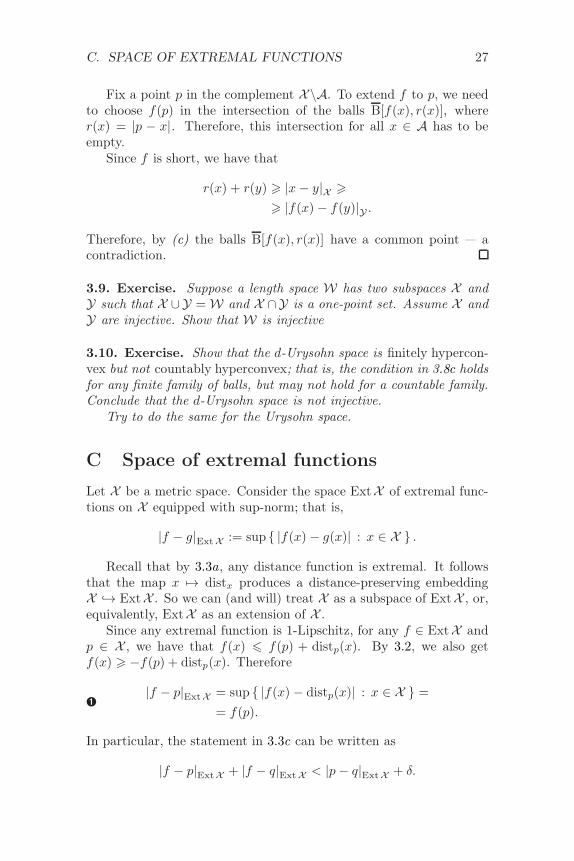
Fix a point p in the complement X\A. To extend f to p, we needto choose f(p) in the intersection of the balls B[f(x), r(x)], wherer(x) = |p − x|. Therefore, this intersection for all x ∈ A has to beempty.
Since f is short, we have that
r(x) + r(y) > |x− y|X >
> |f(x)− f(y)|Y .
Therefore, by (c) the balls B[f(x), r(x)] have a common point — acontradiction.
3.9. Exercise. Suppose a length space W has two subspaces X andY such that X ∪Y = W and X ∩Y is a one-point set. Assume X andY are injective. Show that W is injective
3.10. Exercise. Show that the d-Urysohn space is finitely hypercon-vex but not countably hyperconvex; that is, the condition in 3.8c holdsfor any finite family of balls, but may not hold for a countable family.Conclude that the d-Urysohn space is not injective.
Try to do the same for the Urysohn space.
C Space of extremal functions
Let X be a metric space. Consider the space ExtX of extremal func-tions on X equipped with sup-norm; that is,
|f − g|ExtX := sup |f(x)− g(x)| : x ∈ X .
Recall that by 3.3a, any distance function is extremal. It followsthat the map x 7→ distx produces a distance-preserving embeddingX → ExtX . So we can (and will) treat X as a subspace of ExtX , or,equivalently, ExtX as an extension of X .
Since any extremal function is 1-Lipschitz, for any f ∈ ExtX andp ∈ X , we have that f(x) 6 f(p) + distp(x). By 3.2, we also getf(x) > −f(p) + distp(x). Therefore
➊|f − p|ExtX = sup |f(x) − distp(x)| : x ∈ X =
= f(p).
In particular, the statement in 3.3c can be written as
|f − p|ExtX + |f − q|ExtX < |p− q|ExtX + δ.
28 LECTURE 3. INJECTIVE SPACES
3.11. Exercise. Let X be a metric space. Show that ExtX is compactif and only if so is X .
3.12. Exercise. Describe the set of all extremal functions on a metricspace X and the metric space ExtX in each of the following case:(a) X is a metric space with exactly three points a, b, c such that
|a− b|X = |b− c|X = |c− a|X = 1.
(b) X is a metric space with exactly four points p, q, x, y such that
|p− x|X = |p− y|X = |q − x|X = |q − x|X = 1
and|p− q|X = |x− y|X = 2.
3.13. Proposition. For any metric space X , its extension ExtX isinjective.
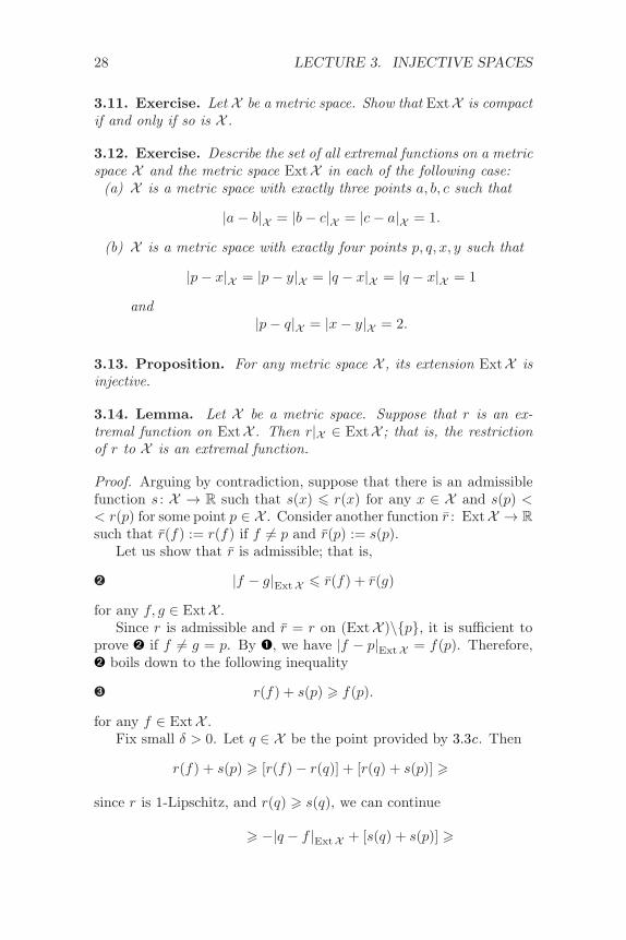
3.14. Lemma. Let X be a metric space. Suppose that r is an ex-tremal function on ExtX . Then r|X ∈ ExtX ; that is, the restrictionof r to X is an extremal function.
Proof. Arguing by contradiction, suppose that there is an admissiblefunction s : X → R such that s(x) 6 r(x) for any x ∈ X and s(p) << r(p) for some point p ∈ X . Consider another function r : ExtX → R
such that r(f) := r(f) if f 6= p and r(p) := s(p).Let us show that r is admissible; that is,
➋ |f − g|ExtX 6 r(f) + r(g)
for any f, g ∈ ExtX .Since r is admissible and r = r on (ExtX )\p, it is sufficient to
prove ➋ if f 6= g = p. By ➊, we have |f − p|ExtX = f(p). Therefore,➋ boils down to the following inequality
➌ r(f) + s(p) > f(p).
for any f ∈ ExtX .Fix small δ > 0. Let q ∈ X be the point provided by 3.3c. Then
r(f) + s(p) > [r(f)− r(q)] + [r(q) + s(p)] >
since r is 1-Lipschitz, and r(q) > s(q), we can continue
> −|q − f |ExtX + [s(q) + s(p)] >
D. INJECTIVE ENVELOPE 29
by ➊ and since s is admissible
> −f(q) + |p− q| >
by 3.3c
> f(p)− δ.
Since δ > 0 is arbitrary, ➌ and ➋ follow.Summarizing: the function r is admissible, r 6 r and r(p) < r(p);
that is, r is not extremal — a contradiction.
Proof of 3.13. Choose an extremal function r : ExtX → R. Set s :=:= r|X . By 3.14, s ∈ ExtX ; that is, s is extremal. By 3.8b, it issufficient to show that
➍ r(f) > |s− f |ExtX
for any f ∈ ExtX .Since r is 1-Lipschitz (3.3b) we have that
s(x) − f(x) = r(x) − |f − x|ExtX 6 r(f).
for any x ∈ X . Since r is admissible we have that
s(x)− f(x) = r(x) − |f − x|ExtX > −r(f).
for any x ∈ X . That is, |s(x) − f(x)| 6 r(f) for any x ∈ X . Recallthat
|s− f |ExtX := sup |s(x)− f(x)| : x ∈ X ;hence ➍ follows.
3.15. Exercise. Let X be a compact metric space. Show that for anytwo points f, g ∈ ExtX lie on a geodesic [pq] with p, q ∈ X .
D Injective envelope
An extension E of a metric space X will be called its injective envelopeif E is an injective space and there is no proper injective subspace ofE that contains X .
Two injective envelopes e : X → E and f : X → F are called equiv-alent if there is an isometry ι : E → F such that f = ι e.3.16. Theorem. For any metric space X , its extension ExtX is aninjective envelope.
30 LECTURE 3. INJECTIVE SPACES
Moreover, any other injective envelope of X is equivalent to ExtX .
Proof. Suppose S ⊂ ExtX is an injective subspace containing X .Since S is injective, there is a short map w : ExtX → S that fixes allpoints in X .
Suppose that w : f 7→ f ′; observe that f(x) > f ′(x) for any x ∈ X .Since f is extremal, f = f ′; that is, w is the identity map and thereforeS = ExtX .
Assume we have another injective envelope e : X → E . Then thereare short maps v : E → ExtX and w : ExtX → E such that x = ve(x)and e(x) = w(x) for any x ∈ X . From above, the composition v w isthe identity on ExtX . In particular, w is distance-preserving.
The composition w v : E → E is a short map that fixes points ine(X ). Since e : X → E is an injective envelope, the composition w vand therefore w are onto. Whence w is an isometry.
3.17. Exercise. Suppose X is a subspace of a metric space U . Showthat the inclusion X → U can be extended to a distance-preservinginclusion ExtX → ExtU .
E Remarks
Injective spaces were introduced by Nachman Aronszajn and PromPanitchpakdi [3]. The injective envelope was introduced by John Isbell[17]. It was rediscovered a couple of times since then; as a resultthe injective envelope has many other names including tight span andhyperconvex hull.
Lecture 4
Space of sets
A Hausdorff distance
Let X be a metric space. Given a subset A ⊂ X , consider the distancefunction to A
distA : X → [0,∞)
defined asdistA(x) := inf
a∈A |a− x|X .
4.1. Definition. Let A and B be two compact subsets of a metricspace X . Then the Hausdorff distance between A and B is defined as
|A−B|HausX := supx∈X
|distA(x) − distB(x)| .
The following observation gives a useful reformulation of the defi-nition:
4.2. Observation. Suppose A and B be two compact subsets of ametric space X . Then |A − B|HausX < R if and only if and only ifB lies in an R-neighborhood of A, and A lies in an R-neighborhoodof B.
Note that the set of all nonempty compact subsets of a metric spaceX equipped with the Hausdorff metric forms a metric space. This newmetric space will be denoted as HausX .
4.3. Exercise. Let X be a metric space. Given a subset A ⊂ Xdefine its diameter as
diamA := supa,b∈A
|a− b|.
31
32 LECTURE 4. SPACE OF SETS
Show thatdiam: HausX → R
is a 2-Lipschitz function; that is,
| diamA− diamB| 6 2·|A−B|HausX
for any two compact nonempty sets A,B ⊂ X .
4.4. Exercise. Let A and B be two compact subsets in the Euclideanplane R2. Assume |A−B|HausR2 < ε.(a) Show that |ConvA−ConvB|HausR2 < ε, where ConvA denoted
the convex hull of A.(b) Is it true that |∂A−∂B|HausR2 < ε, where ∂A denotes the bound-
ary of A.Does the converse hold? That is, assume A and B be two com-pact subsets in R
2 and |∂A − ∂B|HausR2 < ε; is it true that|A−B|HausR2 < ε?
Note that part (a) implies that A 7→ ConvA defines a short mapHausR2 → HausR2.
4.5. Exercise. Let A and B be two compact subsets in metric spaceX . Show that
|A−B|HausX = supf
maxa∈A
f(a) −maxb∈B
f(b) ,
where the least upper bound is taken for all 1-Lipschitz functions f .
B Hausdorff convergence
4.6. Blaschke selection theorem. A metric space X is compact ifand only if so is HausX .
The Hausdorff metric can be used to define convergence. Namely,suppose K1,K2, . . . , and K∞ are compact sets in a metric space X . If|K∞ −Kn|HausX → 0 as n → ∞, then we say that the sequence (Kn)converges to K∞ in the sense of Hausdorff ; or we can say that K∞ isHausdorff limit of the sequence (Kn).
Note that the theorem implies that from any sequence of compactsets in X one can select a subsequence that converges in the sense ofHausdorff; for that reason, it is called a selection theorem.
Proof; “only if” part. Consider the map ι that sends point x ∈ X tothe one-point subset x of X . Note that ι : X → HausX is distance-preserving.
B. HAUSDORFF CONVERGENCE 33
Suppose that A ⊂ X . Note that diamA = 0 if and only if A isa one-point set. Therefore, from Exercise 4.3, it follows that ι(X )is a closed subset of the compact space HausX . Whence ι(X ), andtherefore X , are compact.
To prove the “if” part we will need the following two lemmas.
4.7. Monotone convergence. Let K1 ⊃ K2 ⊃ . . . be a nested se-quence of nonempty compact sets in a metric space X . Then K∞ ==
⋂
n Kn is the Hausdorff limit of Kn; that is, |K∞ −Kn|HausX → 0as n → ∞.
Proof. By finite intersection property, K∞ is a nonempty compact set.If the assertion were false, then there is ε > 0 such that for each n
one can choose xn ∈ Kn such that distK∞(xn) > ε. Note that xn ∈ K1
for each n. Since K1 is compact, there is a partial limit1 x∞ of xn.Clearly, distK∞
(x∞) > ε.On the other hand, since Kn is closed and xm ∈ Kn for m > n,
we get x∞ ∈ Kn for each n. It follows that x∞ ∈ K∞ and thereforedistK∞
(x∞) = 0 — a contradiction.
4.8. Lemma. If X is a compact metric space, then HausX is com-plete.
Proof. Let (Qn) be a Cauchy sequence in HausX . Passing to a sub-sequence of Qn we may assume that
➊ |Qn −Qn+1|HausX 6 110n
for each n.Denote by Kn the closed 1
10n -neighborhood of Qn; that is,
Kn =
x ∈ X : distQn(x) 6 1
10n
Since X is compact so is each Kn.By 4.2, |Qn − Kn|HausX 6 1
10n . From ➊, we get Kn ⊃ Kn+1 foreach n. Set
K∞ =
∞⋂
n=1
Kn.
By the monotone convergence (4.7), |Kn −K∞|HausX → 0 as n → ∞.Since |Qn −Kn|HausX 6 1
10n , we get |Qn −K∞|HausX → 0 as n → ∞— hence the lemma.
1Partial limit is a limit of a subsequence.
34 LECTURE 4. SPACE OF SETS
4.9. Exercise. Let X be a complete metric space and K1,K2, . . . bea sequence of compact sets that converges in the sense of Hausdorff.Show that the union K1 ∪K2 ∪ . . . is a compact closure.
Use this statement to show that in Lemma 4.8 compactness of Xcan be exchanged to completeness.
Proof of “if ” part in 4.6. According to Lemma 4.8, HausX is complete.It remains to show that HausX is totally bounded (1.6d); that is, givenε > 0 there is a finite ε-net in HausX .
Choose a finite ε-net A in X . Denote by B the set of all subsets ofA. Note that B is a finite set in HausX . For each compact set K ⊂ X ,consider the subset K ′ of all points a ∈ A such that distK(a) 6 ε.Observe that K ′ ∈ B and |K −K ′|HausX 6 ε. In other words, B is afinite ε-net in HausX .
4.10. Exercise. Let X be a complete metric space. Show that X isa length space if and only if so is HausX .
C An application
The following statement is called isoperimetric inequality in the plane.
4.11. Theorem. Among the plane figures bounded by closed curvesof length at most ℓ the round disk has the maximal area.
In this section, we will sketch a proof of the isoperimetric inequalitythat uses the Hausdorff convergence. It is based on the followingexercise.
4.12. Exercise. Let C be a subspace of HausR2 formed by all compactconvex subsets in R2. Show that perimeter2 and area are continuouson C. That is, if a sequence of convex compact plane sets Xn convergesto X∞ in the sense of Hausdorff, then
perimXn → perimX∞ and areaXn → areaX∞
as n → ∞.
Semiproof of 4.11. It is sufficient to consider only convex figures ofthe given perimeter; if a figure is not convex, pass to its convex hulland observe that it has a larger area and smaller perimeter.
Note that the selection theorem (4.6) together with the exerciseimply the existence of figure D with perimeter ℓ and maximal area.
2If the set degenerates to a line segment of length ℓ, then its perimeter is definedas 2·ℓ.
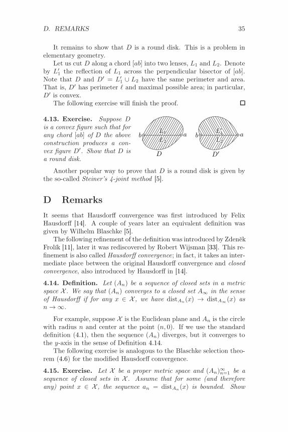
D. REMARKS 35
It remains to show that D is a round disk. This is a problem inelementary geometry.
Let us cut D along a chord [ab] into two lenses, L1 and L2. Denoteby L′
1 the reflection of L1 across the perpendicular bisector of [ab].Note that D and D′ = L′
1 ∪ L2 have the same perimeter and area.That is, D′ has perimeter ℓ and maximal possible area; in particular,D′ is convex.
The following exercise will finish the proof.
L1L1L1L1L1L1L1L1L1L1L1L1L1L1L1L1L1L1L1L1L1L1L1L1L1L1L1L1L1L1L1L1L1L1L1L1L1L1L1L1L1L1L1L1L1L1L1L1L1L1L1L1L1L1L1L1L1L1L1L1L1L1L1L1L1
L2L2L2L2L2L2L2L2L2L2L2L2L2L2L2L2L2L2L2L2L2L2L2L2L2L2L2L2L2L2L2L2L2L2L2L2L2L2L2L2L2L2L2L2L2L2L2L2L2L2L2L2L2L2L2L2L2L2L2L2L2L2L2L2L2
L′
1L′
1L′
1L′
1L′
1L′
1L′
1L′
1L′
1L′
1L′
1L′
1L′
1L′
1L′
1L′
1L′
1L′
1L′
1L′
1L′
1L′
1L′
1L′
1L′
1L′
1L′
1L′
1L′
1L′
1L′
1L′
1L′
1L′
1L′
1L′
1L′
1L′
1L′
1L′
1L′
1L′
1L′
1L′
1L′
1L′
1L′
1L′
1L′
1L′
1L′
1L′
1L′
1L′
1L′
1L′
1L′
1L′
1L′
1L′
1L′
1L′
1L′
1L′
1L′
1
L2L2L2L2L2L2L2L2L2L2L2L2L2L2L2L2L2L2L2L2L2L2L2L2L2L2L2L2L2L2L2L2L2L2L2L2L2L2L2L2L2L2L2L2L2L2L2L2L2L2L2L2L2L2L2L2L2L2L2L2L2L2L2L2L2
D D′
ab ab
4.13. Exercise. Suppose Dis a convex figure such that forany chord [ab] of D the aboveconstruction produces a con-vex figure D′. Show that D isa round disk.
Another popular way to prove that D is a round disk is given bythe so-called Steiner’s 4-joint method [5].
D Remarks
It seems that Hausdorff convergence was first introduced by FelixHausdorff [14]. A couple of years later an equivalent definition wasgiven by Wilhelm Blaschke [5].
The following refinement of the definition was introduced by ZdenekFrolık [11], later it was rediscovered by Robert Wijsman [33]. This re-finement is also called Hausdorff convergence; in fact, it takes an inter-mediate place between the original Hausdorff convergence and closedconvergence, also introduced by Hausdorff in [14].
4.14. Definition. Let (An) be a sequence of closed sets in a metricspace X . We say that (An) converges to a closed set A∞ in the senseof Hausdorff if for any x ∈ X , we have distAn
(x) → distA∞(x) as
n → ∞.
For example, suppose X is the Euclidean plane and An is the circlewith radius n and center at the point (n, 0). If we use the standarddefinition (4.1), then the sequence (An) diverges, but it converges tothe y-axis in the sense of Definition 4.14.
The following exercise is analogous to the Blaschke selection theo-rem (4.6) for the modified Hausdorff convergence.
4.15. Exercise. Let X be a proper metric space and (An)∞n=1 be a
sequence of closed sets in X . Assume that for some (and thereforeany) point x ∈ X , the sequence an = distAn
(x) is bounded. Show
36 LECTURE 4. SPACE OF SETS
that the sequence (An)∞n=1 has a convergent subsequence in the sense
of Definition 4.14.
Lecture 5
Space of spaces
A Gromov–Hausdorff metric
The goal of this section is to cook up a metric space out of met-ric spaces. More precisely, we want to define the so-called Gromov–Hausdorff metric on the set of isometry classes of compact metricspaces. (Being isometric is an equivalence relation, and an isometryclass is an equivalence class with respect to this equivalence relation.)
The obtained metric space will be denoted by GH. Given twometric spaces X and Y, denote by [X ] and [Y] their isometry classes;
that is, X ′ ∈ [X ] if and only if X ′ iso
== X . Pedantically, the Gromov–Hausdorff distance from [X ] to [Y] should be denoted as |[X ]− [Y]|GH;but we will write it as |X − Y|GH and say (not quite correctly) “ |X −− Y|GH is the Gromov–Hausdorff distance from X to Y”. In otherwords, from now on the term metric space might also stand for itsisometry class.
The metric on GH is defined as the maximal metric such that thedistance between subspaces in a metric space is not greater than theHausdorff distance between them. Here is a formal definition:
5.1. Definition. Let X and Y be compact metric spaces. The Gromov–Hausdorff distance |X − Y|GH is defined by the following relation.
Given r > 0, we have that |X −Y|GH < r if and only if there exista metric space Z and subspaces X ′ and Y ′ in Z that are isometricto X and Y respectively and such that |X ′ − Y ′|HausZ < r. (Here|X ′ −Y ′|HausZ denotes the Hausdorff distance between sets X ′ and Y ′
in Z.)
Note that passing to the subspace X ′ ∪Y ′ of Z does not affect thedefinition. Therefore we can always assume that Z is compact.
37
38 LECTURE 5. SPACE OF SPACES
5.2. Theorem. The set of isometry classes of compact metric spacesequipped with Gromov–Hausdorff metric forms a metric space (whichis denoted by GH).
In other words, for arbitrary compact metric spaces X , Y and Zthe following conditions hold:
(a) |X − Y|GH > 0;
(b) |X − Y|GH = 0 if and only if X is isometric to Y;
(c) |X − Y|GH = |Y − X |GH;
(d) |X − Y|GH + |Y − Z|GH > |X − Z|GH.
Note that (a), (c), and the “if”-part of (b) follow directly fromDefinition 5.1. Part (d) will be proved in Section 5B. The “only-if”-part of (b) will be proved in Section 5C.
Recall that a·X denotes X scaled by factor a > 0; that is, a·X isa metric space with the underlying set of X and the metric defined by
|x− y|a·X := a·|x− y|X .
5.3. Exercise. Let X be a compact metric space, P be the one-pointmetric space.
Prove that
(a)
|X − P|GH = 12 · diamX .
(b)
|a·X − b·X |GH = 12 ·|a− b|· diamX .
5.4. Exercise. Let Ar be a rectangle 1 by r in the Euclidean planeand Br be a closed line interval of length r. Show that
|Ar − Br|GH > 110
for all large r.
5.5. Advanced exercise. Let X and Y be compact metric spaces;denote by X and Y their injective envelopes (see the definition on page27). Show that
|X − Y|GH 6 2·|X − Y|GH.
B. APPROXIMATIONS 39
B Approximations
5.6. Definition. Let X and Y be two metric spaces. A relation ≈between points in X and Y is called ε-approximation if the followingconditions hold:
⋄ For any x ∈ X there is y ∈ Y such that x ≈ y.⋄ For any y ∈ Y there is x ∈ X such that x ≈ y.⋄ If for some x, x′ ∈ X and y, y′ ∈ Y we have x ≈ y and x′ ≈ y′,
then∣
∣|x− x′|X − |y − y′|Y∣
∣ < 2·ε.
5.7. Exercise. Let X and Y be two compact metric spaces. Showthat
|X − Y|GH < ε
if and only if there is an ε-approximation between X and Y.In other words |X − Y|GH is the greatest lower bound of values
ε > 0 such that there is an ε-approximation between X and Y.
Proof of 5.2d. Suppose that⋄ ≈1 is a relation between points in X and Y,⋄ ≈2 is a relation between points in Y and Z.
Consider the relation ≈3 between points in X and Z such that x ≈3 zif and only if there is y ∈ Y such that x ≈1 y and y ≈2 z.
It is straightforward to check that if ≈1 is an ε1-approximation and≈2 is an ε2-approximation, then ≈3 is an (ε1 + ε2)-approximation.
Applying 5.7, we get that if
|X − Y|GH < ε1 and |Y − Z|GH < ε2,
then|X − Z|GH < ε1 + ε2.
Hence 5.2d follows.
C Almost isometries
5.8. Definition. Let X and Y be metric spaces and ε > 0. A map1
f : X → Y is called an ε-isometry if f(X ) is an ε-net in Y and
∣
∣|x− x′|X − |f(x)− f(x′)|Y∣
∣ < ε.
1possibly noncontinuous
40 LECTURE 5. SPACE OF SPACES
for any x, x′ ∈ X .
5.9. Exercise. Let X and Y be compact metric spaces.(a) If |X − Y|GH < ε, then there is a 2·ε-isometry f : X → Y.(b) If there is an ε-isometry f : X → Y, then |X − Y|GH < ε.
Proof of the “only if”-part in 5.2b. Let X and Y be compact metricspaces. Suppose that |X − Y|GH < ε for any ε > 0; we need to showthat there is an isometry X → Y.
By 5.9a, for each positive integer n, we can choose a 1n-isometry
fn : X → Y.Since X is compact, we can choose a countable dense set S in X .
Applying the diagonal procedure if necessary, we can assume thatfor every x ∈ S the sequence (fn(x)) converges in Y. Consider thepointwise limit map f∞ : S → Y,
f∞(x) := limn→∞
fn(x)
for every x ∈ S. Since
|fn(x)− fn(x′)|Y <> |x− x′|X ± 1
n,
we have
|f∞(x)− f∞(x′)|Y = limn→∞
|fn(x)− fn(x′)|Y = |x− x′|X
for all x, x′ ∈ S; that is, the map f∞ : S → Y is distance-preserving.Therefore, f∞ can be extended to a distance-preserving map from thewhole X to Y.
The latter can be done by setting
f∞(x) = limn→∞
f∞(xn)
for some sequence of points (xn) in S that converges to x in X . Indeed,if xn → x, then (xn) is Cauchy. Since f∞ is distance-preserving,yn = f∞(xn) is also a Cauchy sequence in Y; therefore it converges.It remains to observe that this construction does not depend on thechoice of the sequence (xn).
This way we obtain a distance-preserving map f∞ : X → Y. Itremains to show that f∞ is surjective; that is, f∞(X ) = Y.
The same argument produces a distance-preserving map g∞ : Y →→ X . If f∞ is not surjective, then neither is the composition f∞ g∞ : Y → Y. So f∞g∞ is a distance-preserving map from a compactspace to itself which is not an isometry. The latter contradicts 1.9.
D. CONVERGENCE 41
D Convergence
The Gromov–Hausdorff metric is used to define Gromov–Hausdorffconvergence. Namely, a sequence of compact metric spaces Xn con-verges to compact metric spaces X∞ in the sense of Gromov–Hausdorffif
|Xn −X∞|GH → 0 as n → ∞.
This convergence is more important than the metric — in all appli-cations, we use only the topology on GH and we do not care about theparticular value of Gromov–Hausdorff distance between spaces. Thefollowing observation follows from 5.9:
5.10. Observation. A sequence of compact metric spaces (Xn) con-verges to X∞ in the sense of Gromov–Hausdorff if and only if there isa sequence εn → 0+ and an εn-isometry fn : Xn → X∞ for each n.
In the following exercises converge means converge in the sense ofGromov–Hausdorff.
5.11. Exercise.
(a) Show that a sequence of compact simply connected length spacescannot converge to a circle.
(b) Construct a sequence of compact simply connected length spacesthat converges to a compact non-simply connected space.
5.12. Exercise.
(a) Show that a sequence of length metrics on the 2-sphere cannotconverge to the unit disk.
(b) Construct a sequence of length metrics on the 3-sphere that con-verges to a unit 3-ball.
Given two metric spaces X and Y, we will write X 6 Y if there isa noncontracting map f : X → Y; that is, if
|x− x′|X 6 |f(x)− f(x′)|Y
for any x, x′ ∈ X .
Further, given ε > 0, we will write X 6 Y + ε if there is a mapf : X → Y such that
|x− x′|X 6 |f(x)− f(x′)|Y + ε
for any x, x′ ∈ X .
42 LECTURE 5. SPACE OF SPACES
E Uniformly totally bonded families
5.13. Definition. A family Q of (isometry classes) of compact metricspaces is called uniformly totally bonded if it meets the following twoconditions:
(a) spaces in Q have uniformly bounded diameters; that is, there isD ∈ R such that
diamX 6 D
for any space X in Q.
(b) For any ε > 0 there is n ∈ N such that any space X in Q admitsan ε-net with at most n points.
5.14. Exercise. Let Q be a family of compact spaces with uniformlybounded diameters. Show that Q is uniformly totally bonded if for anyε > 0 there is n ∈ N such that
packε X 6 n
for any space X in Q.
Fix a real constant C. A Borel measure µ on a metric space X iscalled C-doubling if
µ[B(p, 2·r)] < C ·µ[B(p, r)]
for any point p ∈ X and any r > 0. A Borel measure is called doublingif it is C-doubling for some real constant C.
5.15. Exercise. Let Q(C,D) be the set of all the compact metricspaces with diameter at most D that admit a C-doubling measure.Show that Q(C,D) is totally bounded.
Recall that we write X 6 Y if there is a distance-nondecreasingmap X → Y.
5.16. Exercise.
(a) Let Y be a compact metric space. Show that the set of all spacesX such that X 6 Y is uniformly totally bounded.
(b) Show that for any uniformly totally bounded set Q ⊂ GH thereis a compact space Y such that X 6 Y for any X in Q.
F. GROMOV’S SELECTION THEOREM 43
F Gromov’s selection theorem
The following theorem is analogous to Blaschke selection theorems(4.6).
5.17. Gromov selection theorem. Let Q be a closed subset of GH.Then Q is compact if and only if it is totally bounded.
5.18. Lemma. The space GH is complete.
Let us define gluing of metric spaces that will be used in the proofof the lemma.
Suppose U and V are metric spaces with isometric closed sets A ⊂ Uand A′ ⊂ V ; let ι : A → A′ be an isometry. Consider the space W ofall equivalence classes in U ⊔ V with the equivalence relation given bya ∼ ι(a) for any a ∈ A.
It is straightforward to check that the following defines a metricon W :
|u− u′|W := |u− u′|U|v − v′|W := |v − v′|V|u− v|W := min |u− a|U + |v − ι(a)|V : a ∈ A
where u, u′ ∈ U and v, v′ ∈ V .
The space W is called the gluing of U and V along ι; briefly, wecan write W = U ⊔ι V . If one applies this construction to two copiesof one space U with a set A ⊂ U and the identity map ι : A → A, thenthe obtained space is called the double of U along A; this space can bedenoted by ⊔2
AU .
Note that the inclusions U → W and V → W are distance pre-serving. Therefore we can and will conside U and V as the subspacesof W ; this way the subsets A and A′ will be identified and denotedfurther by A. Note that A = U ∩ V ⊂ W .
Proof. Let (Xn) be a Cauchy sequence in GH. Passing to a sub-sequence if necessary, we can assume that |Xn − Xn+1|GH < 1
2n foreach n. In particular, for each n there is a metric space Vn withdistance preserving inclusions Xn → Vn and Xn+1 → Vn such that
|Xn −Xn+1|HausVn< 1
2n
for each n. Moreover, we may assume that Vn = Xn ∪ Xn+1.
Let us glue V1 to V2 along X2; to the obtained space glue V3 alongX3, and so on. The obtained metric space W has an underlying set
44 LECTURE 5. SPACE OF SPACES
formed by the disjoint union of all Xn such that each inclusion Xn →→ W is distance preserving and
|Xn −Xn+1|HausW < 12n
for each n. In particular,
➊ |Xm −Xn|HausW < 12n−1
if m > n.Denote by W the completion of W . Observe that the union X1 ∪
∪ X2 ∪ . . . ∪ Xn is compact and ➊ implies that it forms a 12n−1 -net in
W . Whence W is compact; see 1.6d and 1.7.Applying Blaschke selection theorem (4.6), we can pass to a subse-
quence of (Xn) that converges in Haus W ; denote its limit by X∞. It re-mains to observe that X∞ is the Gromov–Hausdorff limit of (Xn).
Proof of 5.17; “only if” part. Suppose that there is no sequence εn → 0as described in 5.13. Observe that in this case there is a sequence ofspaces Xn ∈ Q such that
packδ Xn → ∞ as n → ∞
for some fixed δ > 0.Since Q is compact, this sequence has a partial limit, say X∞ ∈ Q.
Observe that packδ X∞ = ∞. Therefore, X∞ is not compact — acontradiction.
“If” part. Suppose sequence (εn) as in the definition of uniformlytotally bonded families (5.13).
Note that diamX 6 ε1 for any X ∈ Q. Given a positive integer nconsider the set of all metric spaces Wn with the number of points atmost n and diameter 6 ε1. Note that Wn is a compact set in GH foreach n.
Further, a subspace formed by a maximal εn-net of any X ∈ Qbelongs to Wn. Therefore, Wn ∩Q is a compact εn-net in Q. That is,Q has a compact ε-net for any ε > 0. Since Q is closed in a completespace GH, it implies that Q is compact.
5.19. Exercise. Show that the space GH is
(a) length,
(b) geodesic.
5.20. Exercise.
G. UNIVERSAL AMBIENT SPACE 45
(a) Show that
|X − Y|GH′ = inf ε > 0 : X 6 Y + ε and Y 6 X + ε
defines a metric on the space of (isometry classes) of compactmetric spaces.
(b) Moreover |∗− ∗|GH′ is equivalent to the Gromov–Hausdorff met-ric; that is,
|Xn −X∞|GH → 0 ⇐⇒ |Xn −X∞|GH′ → 0
as n → ∞.
G Universal ambient space
Recall that a metric space is called universal if it contains an isometriccopy of any separable metric space (in particular, any compact metricspace). Examples of universal spaces include Urysohn space and ℓ∞
— the space of bounded infinite sequences with the metric defined bysup-norm; see 2.9 and 2.3.
The following proposition says that the space W in Definition 5.1can be exchanged to a fixed universal space.
5.21. Proposition. Let U be a universal space. Then for any com-pact metric spaces X and Y we have
|X − Y|GH = inf|X ′ − Y ′|HausU
where the greatest lower bound is taken over all pairs of sets X ′ andY ′ in U which isometric to X and Y respectively.
Proof of 5.21. By the definition (5.1), we have that
|X − Y|GH 6 inf|X ′ − Y ′|HausU;
it remains to prove the opposite inequality.Suppse |X − Y|GH < ε; let X ′, Y ′ and Z be as in 5.1. We can
assume that Z = X ′∪Y ′; otherwise pass to the subspace X ′∪Y ′ of Z.In this case, Z is compact; in particular, it is separable.
Since U is universal, there is a distance-preserving embedding of Zin U ; let us keep the same notation for X ′, Y ′, and their images. Itfollows that
|X ′ − Y ′|HausU < ε,
— hence the result.

46 LECTURE 5. SPACE OF SPACES
5.22. Exercise. Let U∞ be the Urysohn space. Given two compactset A and B in U∞ define
‖A−B‖ = inf|A− ι(B)|Haus U∞,
where the greatest lower bound is taken for all isometrics ι of U∞.Show that ‖∗− ∗‖ defines a pseudometric2 on nonempty compact sub-sets of U∞ and its corresponding metric space is isometric to GH.
H Remarks
Suppose XnGH−−→ X∞, then there is a metric on the disjoint union
X =⊔
n∈N∪∞
Xn
that satisfies the following property:
5.23. Property. The restriction of metric on each Xn and X∞ co-
incides with its original metric and XnH−→ X∞ as subsets in X.
Indeed, since XnGH−−→ X∞, there is a metric on Vn = Xn ⊔X∞ such
that the restriction of metric on each Xn and X∞ coincides with itsoriginal metric and |Xn −X∞|HausVn
< εn for some sequence εn → 0.Gluing all Vn along X∞, we obtain the required space X.
In other words, the metric on X defines the convergence XnGH−−→
GH−−→ X∞. This metric makes it possible to talk about limits of se-quences xn ∈ Xn as n → ∞, as well as weak limits of a sequence ofBorel measures µn on Xn and so on.
For that reason, it is useful to define convergence by specifying themetric on X that satisfies the property for the variation of Hausdorffconvergence described in Section 4D. This approach is very flexible; inparticular, it can be used to define Gromov–Hausdorff convergence ofarbitrary metric spaces (net necessarily compact).
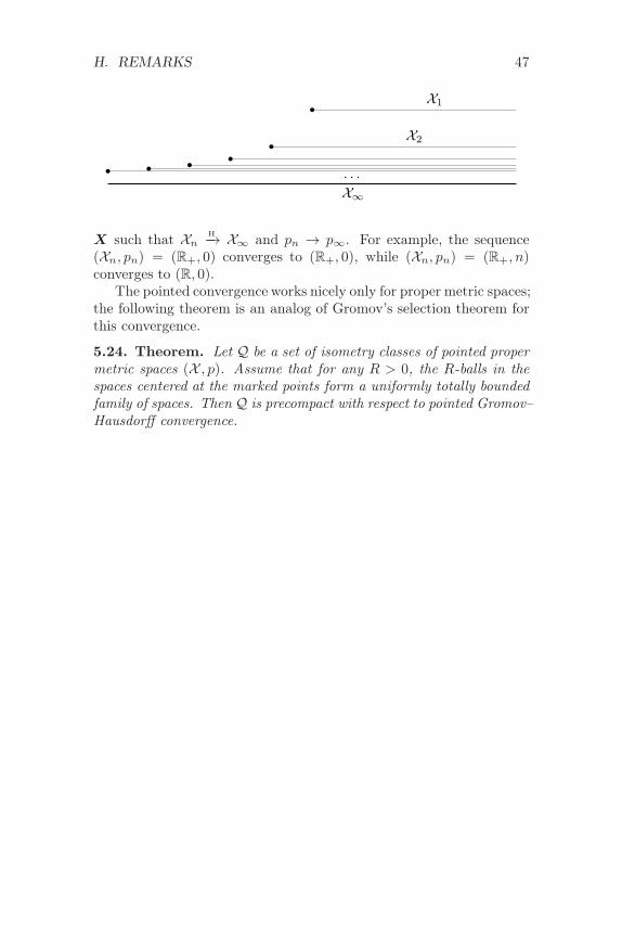
In this case, a limit space for this generalized convergence is notuniquely defined. For example, if each space Xn in the sequence isisometric to the half-line, then its limit might be isometric to the half-line or the whole line. The first convergence is evident and the secondcould be guessed from the diagram.
Often the isometry class of the limit can be fixed by marking a pointpn in each space Xn, it is called pointed Gromov–Hausdorff convergence— we say that (Xn, pn) converges to (X∞, p∞) if there is a metric on
2The value ‖A − B‖ is called Hausdorff distance up to isometry from A to B
in U∞.
H. REMARKS 47
X1
X2
. . .
X∞
X such that XnH−→ X∞ and pn → p∞. For example, the sequence
(Xn, pn) = (R+, 0) converges to (R+, 0), while (Xn, pn) = (R+, n)converges to (R, 0).
The pointed convergence works nicely only for proper metric spaces;the following theorem is an analog of Gromov’s selection theorem forthis convergence.
5.24. Theorem. Let Q be a set of isometry classes of pointed propermetric spaces (X , p). Assume that for any R > 0, the R-balls in thespaces centered at the marked points form a uniformly totally boundedfamily of spaces. Then Q is precompact with respect to pointed Gromov–Hausdorff convergence.
48 LECTURE 5. SPACE OF SPACES
Lecture 6
Ultralimits
Ultralimits provide a very general way to pass to a limit. This proce-dure works for any sequence of metric spaces, its result reminds limitin the sense of Gromov Gausdorff, but has some strange features; forexample, the limit of a constant sequence does not coincide with thisconstant (see 6.10b).
In geometry, ultralimits are used only as a canonical way to passto a convergent subsequence. It is a useful thing in the proofs whereone needs to repeat “pass to convergent subsequence” too many times.
This lecture is based on the introduction to the paper by BruceKleiner and Bernhard Leeb [19].
A Faces of ultrafilters
Recall that N denotes the set of natural numbers, N = 1, 2, . . .6.1. Definition. A finitely additive measure ω on N is called anultrafilter if it satisfies the following condition:(a) ω(N) = 1 and ω(S) = 0 or 1 for any subset S ⊂ N.
An ultrafilter ω is called nonprincipal if in addition(b) ω(F ) = 0 for any finite subset F ⊂ N.
If ω(S) = 0 for some subset S ⊂ N, we say that S is ω-small. Ifω(S) = 1, we say that S contains ω-almost all elements of N.
Classical definition. More commonly, a nonprincipal ultrafilter isdefined as a collection, say F, of sets in N such that
1. if P ∈ F and Q ⊃ P , then Q ∈ F,2. if P,Q ∈ F, then P ∩Q ∈ F,3. for any subset P ⊂ N, either P or its complement is an element
of F.
49
50 LECTURE 6. ULTRALIMITS
4. if F ⊂ N is finite, then F /∈ F.
Setting P ∈ F ⇔ ω(P ) = 1 makes these two definitions equivalent.A nonempty collection of sets F that does not include the empty
set and satisfies only conditions 1 and 2 is called a filter ; if in additionF satisfies condition 3 it is called an ultrafilter. From Zorn’s lemma,it follows that every filter contains an ultrafilter. Thus there is anultrafilter F contained in the filter of all complements of finite sets;clearly, this ultrafilter F is nonprincipal.
Stone–Cech compactification. Given a set S ⊂ N, consider subsetΩS of all ultrafilters ω such that ω(S) = 1. It is straightforward tocheck that the sets ΩS for all S ⊂ N form a topology on the set of ultra-filters on N. The obtained space is called Stone–Cech compactificationof N; it is usually denoted as βN.
Let ωn denotes the principal ultrafilter such that ωn(n) = 1; thatis, ωn(S) = 1 if and only if n ∈ S. Note that n 7→ ωn defines a naturalembedding N → βN. Using the described embedding, we can (andwill) consider N as a subset of βN.
The space βN is the maximal compact Hausdorff space that con-tains N as an everywhere dense subset. More precisely, for any compactHausdorff space X and a map f : N → X there is a unique continuousmap f : βN → X such that the restriction f |N coincides with f .
B Ultralimits of points
Further, we will need the existence of a nonprincipal ultrafilter ω,which we fix once and for all.
Assume (xn) is a sequence of points in a metric space X . Let usdefine the ω-limit of (xn) as the point xω such that for any ε > 0,ω-almost all elements of (xn) lie in B(xω, ε); that is,
ω n ∈ N : |xω − xn| < ε = 1.
In this case, we will write
xω = limn→ω
xn or xn → xω as n → ω.
For example, if ω is the principal ultrafilter such that ωn = 1for some n ∈ N, then xω = xn.
Alternatively, the sequence (xn) can be regarded as a map N → X .In this case, the map N → X can be extended to a continuous mapβN → X from the Stone–Cech compactification βN of N. Then theω-limit xω can be regarded as the image of ω.
B. ULTRALIMITS OF POINTS 51
Note that ω-limits of a sequence and its subsequence may differ.For example, sequence yn = −(−1)n is a subsequence of xn = (−1)n,but for any ultrafilter ω, we have
limn→ω
xn 6= limn→ω
yn.
6.2. Proposition. Let ω be a nonprincipal ultrafilter. Assume (xn)is a sequence of points in a metric space X and xn → xω as n → ω.Then xω is a partial limit of the sequence (xn); that is, there is asubsequence (xn)n∈S that converges to xω in the usual sense.
Proof. Given ε > 0, set Sε = n ∈ N : |xn − xω| < ε .Note that ω(Sε) = 1 for any ε > 0. Since ω is nonprincipal, the set
Sε is infinite. Therefore, we can choose an increasing sequence (nk)such that nk ∈ S 1
kfor each k ∈ N. Clearly, xnk
→ xω as k → ∞.
The following proposition is analogous to the statement that anysequence in a compact metric space has a convergent subsequence; itcan be proved the same way.
6.3. Proposition. Let X be a compact metric space. Then any se-quence of points (xn) in X has a unique ω-limit xω.
In particular, a bounded sequence of real numbers has a uniqueω-limit.
The following lemma is an ultralimit analog of the Cauchy conver-gence test.
6.4. Lemma. Let (xn) be a sequence of points in a complete space X .Assume for each subsequence (yn) of (xn), the ω-limit
yω = limn→ω
yn ∈ X
is defined and does not depend on the choice of subsequence, then thesequence (xn) converges in the usual sense.
Proof. If (xn) is not a Cauchy sequence, then for some ε > 0, there isa subsequence (yn) of (xn) such that |xn − yn| > ε for all n.
It follows that |xω − yω| > ε, a contradiction.
Ultralimits could shorten some proofs in the previous lecture. Thefollowing exercise provides an example.
6.5. Exercise. Use ultralimits to give a shorter proof of 5.2b (page 40).
52 LECTURE 6. ULTRALIMITS
6.6. Exercise. Denote by S the space of bounded sequences of realnumbers. Show that there is a linear functional L : S → R such thatfor any sequence s = (s1, s2, . . . ) ∈ S the image L(s) is a partial limitof s1, s2, . . . .
C Ultralimits of spaces
Recall that ω denotes a nonprincipal ultrafilter on the set of naturalnumbers.
Let Xn be a sequence of metric spaces. Consider all sequences ofpoints xn ∈ Xn. On the set of all such sequences, define a pseudometricby
➊ |(xn)− (yn)| = limn→ω
|xn − yn|Xn.
Note that the ω-limit on the right-hand side is always defined and takesa value in [0,∞]. (The ω-convergence to ∞ is defined analogously tothe usual convergence to ∞).
Set Xω to be the corresponding metric space; that is, the underlyingset of Xω is formed by classes of equivalence of sequences of pointsxn ∈ Xn defined by
(xn) ∼ (yn) ⇔ limn→ω
|xn − yn| = 0
and the distance is defined by ➊.The space Xω is called the ω-limit of Xn. Typically Xω will denote
the ω-limit of sequence Xn; we may also write
Xn → Xω as n → ω or Xω = limn→ω
Xn.
Given a sequence xn ∈ Xn, we will denote by xω its equivalenceclass which is a point in Xω ; it can be written as
xn → xω as n → ω, or xω = limn→ω
xn.
6.7. Observation. The ω-limit of any sequence of metric spaces iscomplete.
Proof. Let Xn be a sequence of metric spaces and Xn → Xω as n → ω.Choose a Cauchy sequence x1, x2, · · · ∈ Xω. Passing to a subsequence,we can assume that |xk − xm|Xω
< 1k
for any k < m.Let us choose a double sequence xn,m ∈ Xn such that for any fixed
m we have xn,m → xm as n → ω. Note that for any k < m the
D. ULTRAPOWER 53
inequality |xn,k − xn,m| < 1k
holds for ω-almost all n. It follows thatwe can choose a nested sequence of sets
N = S1 ⊃ S2 ⊃ . . .
such that
⋄ ω(Sm) = 1 for each m,
⋄⋂
m Sm = ∅, and
⋄ |xn,k − xn,l| < 1k
for k < l 6 m and n ∈ Sm.
Consider the sequence yn = xn,m(n), where m(n) is the largestvalue such that n ∈ Sm(n). Denote by yω ∈ Xω the ω-limit of yn.
Observe that |ym − xn,m| < 1m
for ω-almost all n. It follows that|xm − yω| 6 1
mfor any m. Therefore, xn → yω as n → ∞. That is,
any Cauchy sequence in Xω converges.
6.8. Observation. The ω-limit of any sequence of length spaces isgeodesic.
Proof. If Xn is a sequence of length spaces, then for any sequence ofpairs xn, yn ∈ Xn there is a sequence of 1
n-midpoints zn.
Let xn → xω , yn → yω and zn → zω as n → ω. Note that zω is amidpoint of xω and yω in Xω .
By Observation 6.7, Xω is complete. Applying Lemma 1.20 we getthe statement.
6.9. Exercise. Show that an ultralimit of metric trees is a metrictree.
D Ultrapower
If all the metric spaces in the sequence are identical Xn = X , its ω-limitlimn→ω Xn is denoted by Xω and called ω-power of X .
6.10. Exercise. For any point x ∈ X , consider the constant sequencexn = x and set ι(x) = limn→ω xn ∈ Xω.
(a) Show that ι : X → Xω is distance-preserving embedding. (So wecan and will consider X as a subset of Xω.)
(b) Show that ι is onto if and only if X compact.
(c) Show that if X is proper, then ι(X ) forms a metric componentof Xω; that is, a subset of Xω that lie at a finite distance froma given point.
54 LECTURE 6. ULTRALIMITS
Note that (b) implies that the inclusion X → Xω is not onto ifthe space X is not compact. However, the spaces X and Xω might beisometric; here is an example:
6.11. Exercise. Let X be a countable set with discrete metric; thatis |x− y|X = 1 if x 6= y. Show that
(a) Xω is not isometric to X .
(b) Xω is isometric to (Xω)ω.
6.12. Observation. Let X be a complete metric space. Then Xω isgeodesic space if and only if X is a length space.
Proof. The “if”-part follows from 6.8; it remains to prove the “only-if”-part
Assume Xω is geodesic space. Then any pair of points x, y ∈ Xhas a midpoint zω ∈ Xω. Fix a sequence of points zn ∈ X such thatzn → zω as n → ω.
Note that |x − zn|X → 12 ·|x − y|X and |y − zn|X → 1
2 ·|x − y|X asn → ω. In particular, for any ε > 0, the point zn is an ε-midpoint ofx and y for ω-almost all n. It remains to apply 1.20.
6.13. Exercise. Assume X is a complete length space and p, q ∈ Xcannot be joined by a geodesic in X . Then there are at least two distinctgeodesics between p and q in the ultrapower Xω.
6.14. Exercise. Construct a proper metric space X such that Xω isnot proper; that is, there is a point p ∈ Xω and R < ∞ such that theclosed ball B[p,R]Xω is not compact.
E Tangent and asymptotic spaces
Choose a space X and a sequence of λn > 0. Consider the sequenceof scalings Xn = λn ·X = (X , λn ·|∗ − ∗|X ).
Choose a point p ∈ X and denote by pn the corresponding pointin Xn. Consider the ω-limit Xω of Xn (one may denote it by λω ·X );set pω to be the ω-limit of pn.
If λn → 0 as n → ω, then the metric component of pω in Xω iscalled λω-tangent space at p and denoted by Tλω
p X (or TωpX if λn = n).
If λn → ∞ as n → ω, then the metric component of pω is calledλω-asymptotic space1 and denoted by AsymX or Asymλω X . Note
1Often it is called asymptotic cone despite that it is not a cone in general; thisname is used since in good cases it has a cone structure.
F. REMARKS 55
that the space AsymX and its point pω does not depend on the choiceof p ∈ X .
The following exercise states that the tangent and asymptotic spacesdepend on the sequence λn and a nonprincipal ultrafilter ω.
6.15. Exercise. Construct a metric space X with a point p such thatthe tangent space Tλω
p X depends on the sequence λn and/or ultrafil-ter ω.
For nice spaces, different choices may give the same space.
6.16. Exercise. Let L be the Lobachevsky plane; T = AsymL.(a) Show that T is a complete metric tree.(b) Show that T is one-point homogeneous; that is, given two points
s, t ∈ T there is an isometry of T that maps s to t.(c) Show that T has continuum degree at any point; that is, for any
point t ∈ T the set of connected components of the complementT \t has cardinality continuum.
(d) Prove (a)–(c) if L is Lobachevsky space and/or for the infinite3-regular2 metric tree with unit edge length.
F Remarks
A nonprincipal ultrafilter ω is called selective if for any partition ofN into sets Cαα∈A such that ω(Cα) = 0 for each α, there is a setS ⊂ N such that ω(S) = 1 and S ∩ Cα is a one-point set for eachα ∈ A.
The existence of a selective ultrafilter follows from the continuumhypothesis [30].
For a selective ultrafilter ω, there is a stronger version of Propo-sition 6.2; namely we can assume that the subsequence (xn)n∈S canbe chosen so that ω(S) = 1. So, if needed, one may assume that theultrafilter ω is chosen to be selective and use this stronger version ofthe proposition.
2that is, the degree of any vertex is 3.
56 LECTURE 6. ULTRALIMITS
Appendix A
Semisolutions
1.2. Add four triangle inequalities (1.1d).
1.3;(a). Note that if µ(A) = µ(B) = 0, then |A − B| = 0. Therefore,1.1b does not hold for bounded closed subsets. It is straightforwardto check that for bounded measurable sets the remaining conditionsin 1.1 hold true.
(b). Note that distance from the empty set to the whole plane isinfinite; so the value |A − B| might be infinite. It is straightforwardto check the remaining conditions in 1.1.
1.4. Assume the statement is wrong. Then for any point x ∈ X , thereis a point x′ ∈ X such that
|x− x′| < ρ(x) and ρ(x′) 6ρ(x)
1 + ε.
Consider a sequence of points (xn) such that xn+1 = x′n. Clearly,
|xn+1 − xn| 6ρ(x0)
ε·(1 + ε)nand ρ(xn) 6
ρ(x0)
(1 + ε)n.
Therefore, (xn) is Cauchy. Since X is complete, the sequence (xn)converges; denote its limit by x∞. Since ρ is a continuous function weget
ρ(x∞) = limn→∞
ρ(xn) =
= 0.
The latter contradicts that ρ > 0.
57
58 APPENDIX A. SEMISOLUTIONS
1.5. Let X be completion of X . By the definition, for any y ∈ X thereis a Cauchy sequence (xn) in X that converges to y.
Choose a Cauchy sequence (ym) in X . From above, we can choosepoints xn,m ∈ X such that xn,m → ym for any m. Choose zm = xnm,m
such that |ym − zm| < 1m
. Observe that zm is Cauchy. Therefore, itslimit z∞ lie in X . Finally, show that xm → z∞.
1.7. A compact ε-net N in K contains a finite ε net F . Show and usethat F is a 2·ε-net of K.
1.9. Given a pair of points x0, y0 ∈ K, consider two sequences x0, x1, . . .and y0, y1, . . . such that xn+1 = f(xn) and yn+1 = f(yn) for each n.
Since K is compact, we can choose an increasing sequence of inte-gers nk such that both sequences (xni
)∞i=1 and (yni)∞i=1 converge. In
particular, both are Cauchy; that is,
|xni− xnj
|K, |yni− ynj
|K → 0 as mini, j → ∞.
Since f is non-contracting, we get
|x0 − x|ni−nj || 6 |xni− xnj
|.
It follows that there is a sequence mi → ∞ such that
(∗) xmi→ x0 and ymi
→ y0 as i → ∞.
Setℓn = |xn − yn|K.
Since f is non-contracting, the sequence (ℓn) is nondecreasing.By (∗), ℓmi
→ ℓ0 as mi → ∞. It follows that (ℓn) is a constantsequence.
In particular,
|x0 − y0|K = ℓ0 = ℓ1 = |f(x0)− f(y0)|K
for any pair of points (x0, y0) in K. That is, the map f is distance-preserving and, in particular, injective.
From (∗), we also get that f(K) is everywhere dense. Since K iscompact f : K → K is surjective — hence the result.
Remarks. This is a basic lemma in the introduction to Gromov–Hausdorff distance [see 7.3.30 in 7]. The presented proof is not quitestandard, I learned it from Travis Morrison, a student in my MASSclass at Penn State, Fall 2011.
Note that this exercise implies that any surjective non-expandingmap from a compact metric space to itself is an isometry .
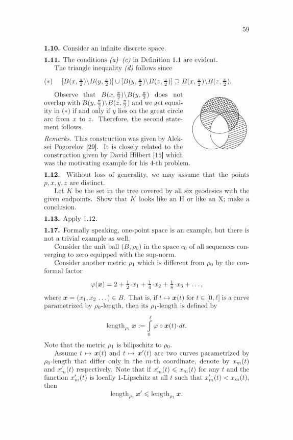
59
1.10. Consider an infinite discrete space.
1.11. The conditions (a)–(c) in Definition 1.1 are evident.The triangle inequality (d) follows since
(∗) [B(x, π2 )\B(y, π2 )] ∪ [B(y, π
2 )\B(z, π2 )] ⊇ B(x, π2 )\B(z, π2 ).
Observe that B(x, π2 )\B(y, π
2 ) does notoverlap with B(y, π
2 )\B(z, π2 ) and we get equal-ity in (∗) if and only if y lies on the great circlearc from x to z. Therefore, the second state-ment follows.
Remarks. This construction was given by Alek-sei Pogorelov [29]. It is closely related to theconstruction given by David Hilbert [15] whichwas the motivating example for his 4-th problem.
1.12. Without loss of generality, we may assume that the pointsp, x, y, z are distinct.
Let K be the set in the tree covered by all six geodesics with thegiven endpoints. Show that K looks like an H or like an X; make aconclusion.
1.13. Apply 1.12.
1.17. Formally speaking, one-point space is an example, but there isnot a trivial example as well.
Consider the unit ball (B, ρ0) in the space c0 of all sequences con-verging to zero equipped with the sup-norm.
Consider another metric ρ1 which is different from ρ0 by the con-formal factor
ϕ(x) = 2 + 12 ·x1 +
14 ·x2 +
18 ·x3 + . . . ,
where x = (x1, x2 . . . ) ∈ B. That is, if t 7→ x(t) for t ∈ [0, ℓ] is a curveparametrized by ρ0-length, then its ρ1-length is defined by
lengthρ1x :=
ℓw
0
ϕ x(t)·dt.
Note that the metric ρ1 is bilipschitz to ρ0.Assume t 7→ x(t) and t 7→ x
′(t) are two curves parametrized byρ0-length that differ only in the m-th coordinate, denote by xm(t)and x′
m(t) respectively. Note that if x′m(t) 6 xm(t) for any t and the
function x′m(t) is locally 1-Lipschitz at all t such that x′
m(t) < xm(t),then
lengthρ1x′ 6 lengthρ1
x.
60 APPENDIX A. SEMISOLUTIONS
Moreover, this inequality is strict if x′m(t) < xm(t) for some t.
Fix a curve x(t), t ∈ [0, ℓ], parametrized by ρ0-length. We canchoose large m so that xm(t) is sufficiently close to 0 for any t. In thiscase, it is easy to construct a function t 7→ x′
m that meets the aboveproperties. It follows that for any curve x(t) in (B, ρ1), we can finda shorter curve x
′(t) with the same endpoints. In particular, (B, ρ1)has no geodesics.
Remarks. This solution was suggested by Fedor Nazarov [23].
1.18. Choose a sequence of positive numbers εn → 0 and an εn-netNn of K for each n. Assume N0 is a one-point set, so ε0 > diamK.Connect each point x ∈ Nk+1 to a point y ∈ Nk by a curve of lengthat most εk.
Consider the union K ′ of all these curves with K; observe that K ′
is compact and path-connected.
Source: This problem was suggested by Eugene Bilokopytov [4].
1.19. Choose a Cauchy sequence (xn) in (X , ‖ ∗ − ∗ ‖); it is sufficientto show that a subsequence of (xn) converges.
Note that the sequence (xn) is Cauchy in (X , | ∗ − ∗ |); denote itslimit by x∞.
Passing to a subsequence, we can assume that ‖xn − xn+1‖ < 12n .
It follows that there is a 1-Lipschitz path γ in (X , ‖ ∗− ∗ ‖) such thatxn = γ( 1
2n ) for each n and x∞ = γ(0).It follows that
‖x∞ − xn‖ 6 length γ|[0, 1
2n] 6
6 12n .
In particular, xn converges to x∞ in (X , ‖ ∗ − ∗ ‖).Source: [16, Corollary]; see also [25, Lemma 2.3].
. . .
p
q1.23. Consider the following subset of R2 equippedwith the induced length metric
X =(
(0, 1]× 0, 1)
∪(
1, 12 , 13 , . . . × [0, 1])
Note that X is locally compact and geodesic.Its completion X is isometric to the closure of X equipped with
the induced length metric. Note that X is obtained from X by addingtwo points p = (0, 0) and q = (0, 1).
Observe that the point p admits no compact neighborhood in Xand there is no geodesic connecting p to q in X .
Source: [6, I.3.6(4)].

61
1.24. If such a number does not exist, then the ranges of averagedistance functions have an empty intersection. Since X is a compactlength-metric space, the range of any continuous function on X is aclosed interval. By 1-dimensional Helly’s theorem, there is a pair ofsuch range intervals that do not intersect. That is, for two point-arrays(x1, . . . , xn) and (y1, . . . , ym) and their average distance functions
f(z) = 1n·∑
i
|xi − z|X and h(z) = 1m·∑
j
|yj − z|X ,
we have
(∗) min f(z) : z ∈ X > max h(z) : z ∈ X .
Note that
1m·∑
j
f(yj) =1
m·n ·∑
i,j
|xi − yj |X = 1n·∑
i
h(xi);
that is, the average value of f(yj) coincides with the average value ofh(xi), which contradicts (∗).Remarks. The value ℓ is uniquely defined; it is called the rendezvousvalue of X . This is a result of Oliver Gross [13].
2.2. By Frechet lemma (2.1) we can identify K with a compact subsetof ℓ∞.
Denote by L = ConvK — it is defined as the minimal convex closedset in ℓ∞ that contains K. (In other words, L is the minimal closedset containing K such that if x, y ∈ L, then t·x+(1− t)·y ∈ L for anyt ∈ [0, 1].)
Observe that L is a length space. It remains to show that L iscompact.
By construction, L is a closed subset of ℓ∞; in particular, it is acomplete space. By 1.6d , it remains to show that L is totally bounded.
Recall that Minkowski sum A+B of two sets A and B in a vectorspace is defined by
A+B = a+ b : a ∈ A, b ∈ B .
Observe that the Minkowski sum of two convex sets is convex.Denote by Bε the closed ε-ball in ℓ∞ centered at the origin. Choose
a finite ε-net N in K for some ε > 0. Note that P = ConvN is a convexpolyhedron; in particular, ConvN is compact.
Observe that N+Bε is closed ε-neighborhood of N . It follows thatN + Bε ⊃ K and therefore P + Bε ⊃ L. In particular, P is a 2·ε-net
62 APPENDIX A. SEMISOLUTIONS
in L; since P is compact and ε > 0 is arbitrary, L is totally bounded(see 1.7).
Remark. Alternatively, one may use that the injective envelope of acompact space is compact ; see 3.5b, 3.11, and 3.13.
2.3. Modify the proof of 2.1.
2.10. Choose a separable space X that has an infinite number of geo-desics between a pair of points with the given distance between them;say a square in R2 with ℓ∞-metric will do. Apply to X universality ofUrysohn space (2.9).
2.11. First let us prove the following claim:
⋄ Suppose f : K → R is an extension function defined on a compactsubset K of the Urysohn space U . Then there is a point p ∈ Usuch that |p− x| = f(x) for any x ∈ K.
Without loss of generality, we may assume that f(x) > 0 for anyx ∈ K. Since K is compact, we may fix ε > 0 such that f(x) > ε.
Consider the sequence εn = ε100·2n . Choose a sequence of εn-nets
Nn ⊂ K. Applying universality of U recursively, we may choose apoint pn such that |pn − x| = f(x) for any x ∈ Nn and |pn − pn−1| == 10·εn−1. Observe that the sequence (pn) is Cauchy and its limit pmeets |p− x| = f(x) for any x ∈ K.
Now, choose a sequence of points (xn) in S. Applying the claim,we may extend the map from K to K ∪ x1, further to K ∪ x1, x2,and so on. As a result, we extend the distance-preserving map f tothe whole sequence (xn). It remains to extend it continuously to thewhole space S.
2.13. It is sufficient to show that any compact subspace K of theUrysohn space U can be contracted to a point.
Note that any compact space K can be extended to a contractiblecompact space K′; for example, we may embed K into ℓ∞ and pass toits convex hull, as it was done in 2.2.
By 2.17, there is an isometric embedding of K′ that agrees withthe inclusion K → U . Since K is contractible in K′, it is contractiblein U .
A better way. One can contract the whole Urysohn space using thefollowing construction.
Note that points in X∞ constructed in the proof of 2.6 can bemultiplied number t ∈ [0, 1] — simply multiply each function by t.That defines a map
λt : X∞ → X∞

63
that scales all distances by factor t. The map λt can be extended tothe completion of X∞, which is isometric to Ud (or U).
Observe that the map λ1 is the identity and λ0 maps the wholespace to a single point, say x0 — this is the only point of X0. Further,note that (t, p) 7→ λt(p) is a continuous map; in particular, Ud and Uare contractible.
As a bonus, observe that for any point p ∈ Ud the curve t 7→ λt(p)is a geodesic path from p to x0.
Source: [12, (d) on page 82].
2.16; (a) and (b). Observe that L and M satisfy the definition ofd-Urysohn space and apply the uniqueness (2.14). Note that
ℓ = diamL = min2·r, d.
(c). Use (a), maybe twice.
2.18; (a). The euclidean plane is homogeneous in every sense.
(b). The Hilbert space ℓ2 is finite-set homogeneous, but not compactset homogeneous, nor countable homogeneous.
(c). The space ℓ∞ is 1-point homogeneous, but not 2-point homoge-neous. Try to show that there is no isometry of ℓ∞ such that
(0, 0, 0, . . . ) 7→ (0, 0, 0, . . . ),
(1, 1, 1, . . . ) 7→ (1, 0, 0, . . . ).
(d). The space ℓ1 is 1-point homogeneous, but not 2-point homoge-neous. Try to show that there is no isometry of ℓ∞ such that
(0, 0, 0, . . . ) 7→ (0, 0, 0, . . . ),
(2, 0, 0 . . . ) 7→ (1, 1, 0, . . . ).
3.2. Note that if c < 0, then r > s. The latter is impossible since r isextremal and s is admissible.
Observe that the function r = min r, s+ c is admissible. Indeed,choose x, y ∈ X . If r(x) = r(x) and r(y) = r(y), then
r(x) + r(y) = r(x) + r(y) > |x− y|.
Further, if r(x) = s(x) + c, then
r(x) + r(y) > [s(x) + c] + [s(y)− c] =
= s(x) + s(y) >
> |x− y|.
64 APPENDIX A. SEMISOLUTIONS
Since r is extremal, we have r = r; that is, r 6 s+ c.
3.5. Choose an injective space Y.(a). Fix a Cauchy sequence (xn) in Y; we need to show that it has
a limit x∞ ∈ Y. Consider metric on X = N ∪ ∞ defined by
|m− n|X := |xm − xn|Y ,|m−∞|X := lim
n→∞|xm − xn|Y .
Since the sequence is Cauchy, so is the sequence ℓn = |xm − xn|Y forany m. Therefore, the last limit is defined.
By construction, the map n 7→ xn is distance-preserving on N ⊂ X .Since Y is injective, this map can be extended to ∞ as a short map;set ∞ 7→ x∞. Since |xn − x∞|Y 6 |n −∞|X and |n −∞|X → 0, weget that xn → x∞ as n → ∞.
(b). Applying the definition of injective space, we get a midpointfor any pair of points in Y. By (a), Y is a complete space. It remainsto apply 1.20b.
(c). Let k : Y → ℓ∞(Y) be the Kuratowski embedding (2.4). Ob-serve that ℓ∞(Y) is contractible; in particular, there is a homotopykt : Y → ℓ∞(Y) such that k0 = k and k1 is a constant map. (In fact,one can take kt = (1 − t)·k.)
Since k is distance-preserving and Y is injective, there is a shortmap f : ℓ∞(Y) → Y such that the composition f k is the identitymap on Y. The composition f kt : Y → Y is a needed homotopy.
3.6. Suppose that a short map f : A → Y is defined on a subset Aof a metric space X . We need to construct a short extension F off . Without loss of generality, we may assume that A 6= ∅, otherwisemap the whole X to a single point. By Zorn’s lemma, it is sufficientto enlarge A by a single point x /∈ A.
(a). Suppose Y = R. Set
F (x) = inf f(a)− |a− x| : a ∈ A .
Observe that F is short and F (a) = f(a) for any a ∈ A.
(b). Suppose Y is a complete metric tree. Fix points p ∈ X and q ∈ Y.Given a point a ∈ A, let xa ∈ B[f(a), |a − p|] be the point closest tof(x). Note that xa ∈ [q f(a)] and either xa = q or xa lies on distance|a− p| from f(a).
Note that the geodesics [q xa] are nested; that is, for any a, b ∈ Awe have either [q xa] ⊂ [q xb] or [q xb] ⊂ [q xa]. Moreover, in the firstcase we have |xb−f(a)| 6 |p−a| and in the second |xa−f(b)| 6 |p−b|.
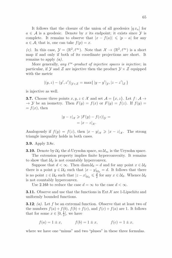
65
It follows that the closure of the union of all geodesics [q xa] fora ∈ A is a geodesic. Denote by x its endpoint; it exists since Y iscomplete. It remains to observe that |x − f(a)| 6 |p − a| for anya ∈ A; that is, one can take f(p) = x.
(c). In this case, Y = (R2, ℓ∞). Note that X → (R2, ℓ∞) is a shortmap if and only if both of its coordinate projections are short. Itremains to apply (a).
More generally, any ℓ∞-product of injective spaces is injective; inparticular, if Y and Z are injective then the product Y × Z equippedwith the metric
|(y, z)− (y′, z′)|Y×Z = max |y − y′|Y , |z − z′|Z
is injective as well.
3.7. Choose three points x, y, z ∈ X and set A = x, z. Let f : A →→ Y be an isometry. Then F (y) = f(x) or F (y) = f(z). If f(y) == f(x), then
|y − z|X > |F (y)− f(z)|Y =
= |x− z|X .
Analogously if f(y) = f(z), then |x − y|X > |x − z|X . The strongtriangle inequality holds in both cases.
3.9. Apply 3.8c.
3.10. Denote by Ud the d-Urysohn space, so U∞ is the Urysohn space.The extension property implies finite hyperconvexity. It remains
to show that Ud is not countably hyperconvex.Suppose that d < ∞. Then diamUd = d and for any point x ∈ Ud
there is a point y ∈ Ud such that |x − y|Ud= d. It follows that there
is no point z ∈ Ud such that |z− x|Ud6 d
2 for any x ∈ Ud. Whence Ud
is not countably hyperconvex.Use 2.16b to reduce the case d = ∞ to the case d < ∞.
3.11. Observe and use that the functions in ExtX are 1-Lipschitz anduniformly bounded functions.
3.12; (a). Let f be an extremal function. Observe that at least two ofthe numbers f(a)+ f(b), f(b)+ f(c), and f(c)+ f(a) are 1. It followsthat for some x ∈ [0, 12 ], we have
f(a) = 1± x, f(b) = 1± x, f(c) = 1± x,
where we have one “minus” and two “pluses” in these three formulas.
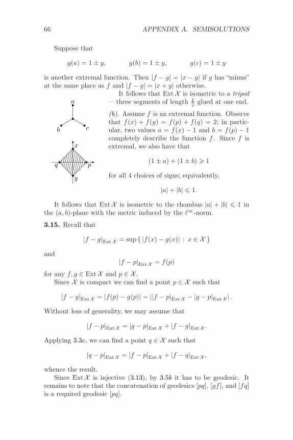
66 APPENDIX A. SEMISOLUTIONS
Suppose that
g(a) = 1± y, g(b) = 1± y, g(c) = 1± y
is another extremal function. Then |f − g| = |x − y| if g has “minus”at the same place as f and |f − g| = |x+ y| otherwise.
a
b c
x
y
pq
It follows that ExtX is isometric to a tripod— three segments of length 1
2 glued at one end.
(b). Assume f is an extremal function. Observethat f(x) + f(y) = f(p) + f(q) = 2; in partic-ular, two values a = f(x) − 1 and b = f(p) − 1completely describe the function f . Since f isextremal, we also have that
(1± a) + (1± b) > 1
for all 4 choices of signs; equivalently,
|a|+ |b| 6 1.
It follows that ExtX is isometric to the rhombus |a| + |b| 6 1 inthe (a, b)-plane with the metric induced by the ℓ∞-norm.
3.15. Recall that
|f − g|ExtX = sup |f(x)− g(x)| : x ∈ X
and|f − p|ExtX = f(p)
for any f, g ∈ ExtX and p ∈ X .Since X is compact we can find a point p ∈ X such that
|f − g|ExtX = |f(p)− g(p)| = ||f − p|ExtX − |g − p|ExtX | .
Without loss of generality, we may assume that
|f − p|ExtX = |g − p|ExtX + |f − g|ExtX .
Applying 3.3c, we can find a point q ∈ X such that
|q − p|ExtX = |f − p|ExtX + |f − q|ExtX ,
whence the result.Since ExtX is injective (3.13), by 3.5b it has to be geodesic. It
remains to note that the concatenation of geodesics [pq], [gf ], and [fq]is a required geodesic [pq].
67
3.17. Show that there is a pair of short maps ExtX → ExtU → ExtXsuch that their composition is identity of X . Make a conclusion.
4.3. Suppose that |A−B|HausX < r. Choose a pair of points a, a′ ∈ Aon maximal distance from each other. Observe that there are pointsb, b′ ∈ B such that |a− b|X , |a′ − b′|X < r. Whence
|a− a′|X − |b− b′|X 6 2·r
and therefore
diamA− diamB 6 2·|A−B|HausX .
It remains to swap A and B and repeat the argument.
4.4; (a). Denote by Ar the closed r-neighborhood of a set A ⊂ R2.Observe that
(ConvA)r = Conv(Ar),
and try to use it.
(b). The answer is “no” in both parts.For the first part let A be a unit disk and B a finite ε-net in A.
Evidently, |A−B|HausR2 < ε, but |∂A− ∂B|HausR2 ≈ 1.For the second part take A to be a unit disk and B = ∂A to
be its boundary circle. Note that ∂A = ∂B; in particular, |∂A −− ∂B|HausR2 = 0 while |A−B|HausR2 = 1.
Remark. There is the so-called lakes of Wada — an example of three(and more) open bounded topological disks in the plane that haveidentical boundaries. It can be used to construct more interestingexamples for (b).
4.9. Show that for any ε > 0 there is a positive integer N such that⋃
n6N Kn is an ε-net in the union⋃
n Kn. Observe that⋃
n6N Kn iscompact and apply 1.7.
4.10; “if ” part. Choose two compact sets A,B ⊂ X ; suppose that|A−B|HausX < r.
Choose finite ε-nets a1, . . . am ⊂ A and b1, . . . bn ⊂ B. Foreach pair ai, bj construct a constant-speed path γi,j from ai to bj suchthat
length γi,j < |ai − bj | + ε.
Set
C(t) = γi,j(t) : |ai − bj|X < r + ε .Observe that C(t) is finite; in particular, it is compact.
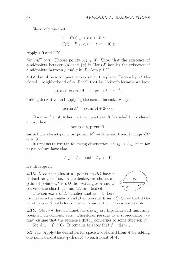
68 APPENDIX A. SEMISOLUTIONS
Show and use that
|A− C(t)|X < t·r + 10·ε,|C(t)−B|X < (1− t)·r + 10·ε.
Apply 4.9 and 1.20.
“only-if” part. Choose points p, q ∈ X . Show that the existence ofε-midpoints between p and q in HausX implies the existence ofε-midpoints between p and q in X . Apply 1.20.
4.12. Let A be a compact convex set in the plane. Denote by Ar theclosed r-neighborhood of A. Recall that by Steiner’s formula we have
areaAr = areaA+ r· perimA+ π·r2.
Taking derivative and applying the coarea formula, we get
perimAr = perimA+ 2·π·r.
Observe that if A lies in a compact set B bounded by a closedcurve, then
perimA 6 perimB.
Indeed the closest-point projection R2 → A is short and it maps ∂Bonto ∂A.
It remains to use the following observation: if An → A∞, then forany r > 0 we have that
Ar∞ ⊃ An and A∞ ⊂ Ar
n
for all large n.
Dab
αβ
4.13. Note that almost all points on ∂D have adefined tangent line. In particular, for almost allpairs of points a, b ∈ ∂D the two angles α and βbetween the chord [ab] and ∂D are defined.
The convexity of D′ implies that α = β; herewe measure the angles α and β on one side from [ab]. Show that if theidentity α = β holds for almost all chords, then D is a round disk.
4.15. Observe that all functions distAnare Lipschitz and uniformly
bounded on compact sets. Therefore, passing to a subsequence, wemay assume that the sequence distAn
converges to some function f .Set A∞ = f−10. It remains to show that f = distA∞
.
5.3; (a). Apply the definition for space Z obtained from X by addingone point on distance 1
2 · diamX to each point of X .
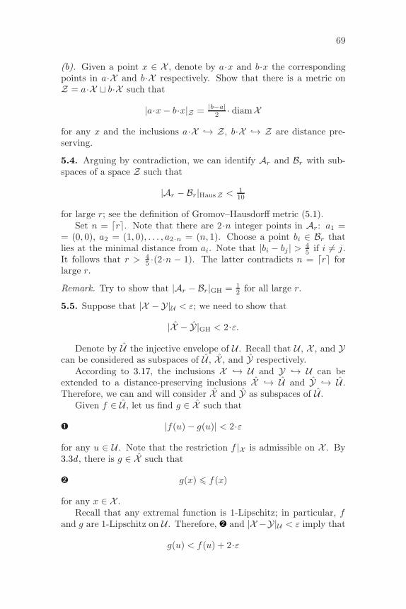
69
(b). Given a point x ∈ X , denote by a·x and b·x the correspondingpoints in a·X and b·X respectively. Show that there is a metric onZ = a·X ⊔ b·X such that
|a·x− b·x|Z = |b−a|2 · diamX
for any x and the inclusions a·X → Z, b·X → Z are distance pre-serving.
5.4. Arguing by contradiction, we can identify Ar and Br with sub-spaces of a space Z such that
|Ar − Br|HausZ < 110
for large r; see the definition of Gromov–Hausdorff metric (5.1).Set n = ⌈r⌉. Note that there are 2·n integer points in Ar: a1 =
= (0, 0), a2 = (1, 0), . . . , a2·n = (n, 1). Choose a point bi ∈ Br thatlies at the minimal distance from ai. Note that |bi − bj | > 4
5 if i 6= j.It follows that r > 4
5 ·(2·n − 1). The latter contradicts n = ⌈r⌉ forlarge r.
Remark. Try to show that |Ar − Br|GH = 12 for all large r.
5.5. Suppose that |X − Y|U < ε; we need to show that
|X − Y|GH < 2·ε.
Denote by U the injective envelope of U . Recall that U , X , and Ycan be considered as subspaces of U , X , and Y respectively.
According to 3.17, the inclusions X → U and Y → U can beextended to a distance-preserving inclusions X → U and Y → U .Therefore, we can and will consider X and Y as subspaces of U .
Given f ∈ U , let us find g ∈ X such that
➊ |f(u)− g(u)| < 2·ε
for any u ∈ U . Note that the restriction f |X is admissible on X . By3.3d , there is g ∈ X such that
➋ g(x) 6 f(x)
for any x ∈ X .Recall that any extremal function is 1-Lipschitz; in particular, f
and g are 1-Lipschitz on U . Therefore, ➋ and |X −Y|U < ε imply that
g(u) < f(u) + 2·ε
70 APPENDIX A. SEMISOLUTIONS
for any u ∈ U . By 3.2, we also have
g(u) > f(u)− 2·ε
for any u ∈ U . Whence ➊ follows.It follows that Y lies in a 2·ε-neighborhood of X in U . The same
way we show that X lies in a 2·ε-neighborhood of Y in U . The lattermeans that |X − Y|Haus U < 2·ε, and therefore |X − Y|GH < 2·ε.Remark. This problem was discussed by Urs Lang, Mael Pavon, andRoger Zust [21, 3.1]. They also show that the constant 2 is opti-
ℓ1ℓ1ℓ1ℓ1ℓ1ℓ1ℓ1ℓ1ℓ1ℓ1ℓ1ℓ1ℓ1ℓ1ℓ1ℓ1ℓ1ℓ1ℓ1ℓ1ℓ1ℓ1ℓ1ℓ1ℓ1ℓ1ℓ1ℓ1ℓ1ℓ1ℓ1ℓ1ℓ1ℓ1ℓ1ℓ1ℓ1ℓ1ℓ1ℓ1ℓ1ℓ1ℓ1ℓ1ℓ1ℓ1ℓ1ℓ1ℓ1ℓ1ℓ1ℓ1ℓ1ℓ1ℓ1ℓ1ℓ1ℓ1ℓ1ℓ1ℓ1ℓ1ℓ1ℓ1ℓ1
1
1
1
1
s
s
4
mal. To see this, look at the injective envelopes of two 4-point metricspaces shown on the diagram and observe that the Gromov–Hausdorffdistance between the 4-point metric spaces is 1, while the distancebetween their injective envelopes approaches 2 as s → ∞.
5.7; only-if part. Let us identify X and Y with subspaces of a metricspace Z such that
|X − Y|HausZ < ε.
Set x ≈ y if and only if |x− y|Z < ε. It remains to check that ≈ isan ε-approximation.
If part. Show that we can assume that
R = (x, y) ∈ X × Y : x ≈ y
is a compact subset of X × Y. Conclude that∣
∣|x− x′|X − |y − y′|Y∣
∣ < 2·ε′
for some ε′ < ε.Show that there is a metric on Z = X ⊔Y such that the inclusions
X → Z and Y → Z are distance preserving and |x−y|Z = ε′ if x ≈ y.Conclude that
|X − Y|HausZ 6 ε′ < ε.
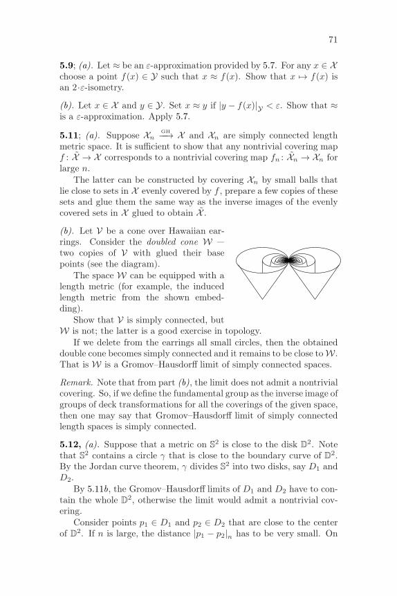
71
5.9; (a). Let ≈ be an ε-approximation provided by 5.7. For any x ∈ Xchoose a point f(x) ∈ Y such that x ≈ f(x). Show that x 7→ f(x) isan 2·ε-isometry.
(b). Let x ∈ X and y ∈ Y. Set x ≈ y if |y − f(x)|Y < ε. Show that ≈is a ε-approximation. Apply 5.7.
5.11; (a). Suppose XnGH−−→ X and Xn are simply connected length
metric space. It is sufficient to show that any nontrivial covering mapf : X → X corresponds to a nontrivial covering map fn : Xn → Xn forlarge n.
The latter can be constructed by covering Xn by small balls thatlie close to sets in X evenly covered by f , prepare a few copies of thesesets and glue them the same way as the inverse images of the evenlycovered sets in X glued to obtain X .
(b). Let V be a cone over Hawaiian ear-rings. Consider the doubled cone W —two copies of V with glued their basepoints (see the diagram).
The space W can be equipped with alength metric (for example, the inducedlength metric from the shown embed-ding).
Show that V is simply connected, butW is not; the latter is a good exercise in topology.
If we delete from the earrings all small circles, then the obtaineddouble cone becomes simply connected and it remains to be close to W .That is W is a Gromov–Hausdorff limit of simply connected spaces.
Remark. Note that from part (b), the limit does not admit a nontrivialcovering. So, if we define the fundamental group as the inverse image ofgroups of deck transformations for all the coverings of the given space,then one may say that Gromov–Hausdorff limit of simply connectedlength spaces is simply connected.
5.12, (a). Suppose that a metric on S2 is close to the disk D2. Notethat S2 contains a circle γ that is close to the boundary curve of D2.By the Jordan curve theorem, γ divides S2 into two disks, say D1 andD2.
By 5.11b, the Gromov–Hausdorff limits of D1 and D2 have to con-tain the whole D2, otherwise the limit would admit a nontrivial cov-ering.
Consider points p1 ∈ D1 and p2 ∈ D2 that are close to the centerof D2. If n is large, the distance |p1 − p2|n has to be very small. On
72 APPENDIX A. SEMISOLUTIONS
the other hand, any curve from p1 to p2 must cross γ, so it has lengthabout 2 — a contradiction.
5.14. Apply 1.8.
5.15. Choose a space X in Q(C,D), denote a C-doubling measureby µ. Without loss of generality, we may assume that µ(X ) = 1.
The doubling condition implies that
µ[B(p, D2n )] >
1Cn
for any point x ∈ X . It follows that
pack D2n
X 6 Cn.
By 1.8, for any ε > D2n−1 , the space X admits an ε-net with at most
Cn points. Whence Q(C,D) is uniformly totally bounded.
5.16; (a). Choose ε > 0. Since Y is compact, we can choose a finiteε-net y1, . . . , yn in Y.
Suppose f : X → Y be a distance-nondecreasing map. Choose onepoint xi in each nonempty subset Bi = f−1[B(yi, ε)]. Note that thesubset Bi has diameter at most 2·ε and
X =⋃
i
Bi.
Therefore, the set of points xi is a 2·ε-net in X .
(b). Let Q be a uniformly totally bounded family of spaces. Supposethat each space in Q has an 1
2n -net with at most Mn points; we mayassume that M0 = 1.
Consider the space Y of all infinite integer sequences m0,m1, . . .such that 1 6 mn 6 Mn for any n. Given two sequences (ℓn), and(mn) of points in Y, set
|(ℓn)− (mn)|Y = C2n ,
where n is the minimal index such that ℓn 6= mn and C is a positiveconstant.
Observe that Y is compact. Indeed it is complete and the sequenceswith constant tails, starting from index n, form a finite C
2n -net in Y.Given a space X in Q, choose a sequence of 1
2n nets Nn ⊂ Xfor each n. We can assume that |Nn| 6 Mn; let us label the pointsin Nn by 1, . . . ,Mn. Consider the map f : X → Y defined byf : x → (m1(x),m2(x), . . . ) where mn(x) is the label of a point in Nn
that lies on the distance < 12n from x.
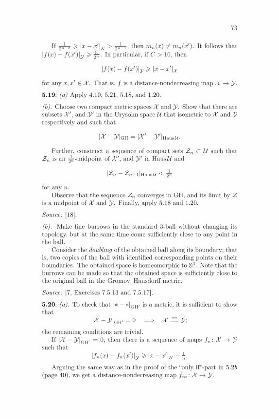
73
If 12n−2 > |x − x′|X > 1
2n−1 , then mn(x) 6= mn(x′). It follows that
|f(x)− f(x′)|Y > C2n . In particular, if C > 10, then
|f(x)− f(x′)|Y > |x− x′|X
for any x, x′ ∈ X . That is, f is a distance-nondecreasing map X → Y.
5.19; (a) Apply 4.10, 5.21, 5.18, and 1.20.
(b). Choose two compact metric spaces X and Y. Show that there aresubsets X ′, and Y ′ in the Urysohn space U that isometric to X and Yrespectively and such that
|X − Y|GH = |X ′ − Y ′|HausU .
Further, construct a sequence of compact sets Zn ⊂ U such thatZn is an 1
2n -midpoint of X ′, and Y ′ in HausU and
|Zn −Zn+1|HausU < 12n
for any n.Observe that the sequence Zn converges in GH, and its limit by Z
is a midpoint of X and Y. Finally, apply 5.18 and 1.20.
Source: [18].
(b). Make fine burrows in the standard 3-ball without changing itstopology, but at the same time come sufficiently close to any point inthe ball.
Consider the doubling of the obtained ball along its boundary; thatis, two copies of the ball with identified corresponding points on theirboundaries. The obtained space is homeomorphic to S3. Note that theburrows can be made so that the obtained space is sufficiently close tothe original ball in the Gromov–Hausdorff metric.
Source: [7, Exercises 7.5.13 and 7.5.17].
5.20; (a). To check that |∗ − ∗|GH′ is a metric, it is sufficient to showthat
|X − Y|GH′ = 0 =⇒ X iso
== Y;the remaining conditions are trivial.
If |X − Y|GH′ = 0, then there is a sequence of maps fn : X → Ysuch that
|fn(x)− fn(x′)|Y > |x− x′|X − 1
n.
Arguing the same way as in the proof of the “only if”-part in 5.2b(page 40), we get a distance-nondecreasing map f∞ : X → Y.
74 APPENDIX A. SEMISOLUTIONS
The same way we can construct a distance-nondecreasing mapg∞ : Y → X .
By 1.9, the compositions f∞ g∞ : Y → Y and g∞ f∞ : X → Xare isometries. Therefore, f∞ and g∞ are isometries as well.
(b). The implication
|Xn −X∞|GH → 0 ⇒ |Xn −X∞|GH′ → 0
follows from 5.9a.Now suppose |Xn − X∞|GH′ → 0. Show that Xn is a uniformly
totally bonded family.If |Xn −X∞|GH 6→ 0, then we can pass to a subsequence such that
|Xn − X∞|GH > ε for some ε > 0. By Gromov selection theorem,we can assume that Xn converges in the sense of Gromov–Hausdorff.From the first implication, the limit X ′
∞ has to be isometric to X∞;on the other hand, |X ′
∞ −X∞|GH > ε — a contradiction.
5.22. Apply 2.17 and 5.21.
6.5. Suppose that fn : X → Y is a 1n-isometry between compact spaces
for each n ∈ N. Consider the ω-limit fω of fn,
fω(x) = limn→ω
fn(x);
according to 6.3, fω is defined. Since
|fn(x) − fn(x′)| ≶ |x− x′| ± 1
n
we get that
|fω(x) − fω(x′)| = |x− x′|
for any x, x′ ∈ X ; that is, fω is distance-preserving. Further, since fnis a 1
n-isometry, for any y ∈ Y there is xm such that |fn(xn)− y| 6 1
n.
Therefore,
fω(xω) = y,
where xω is the ω-limit of xn; that is, fω is onto. It follows thatfω : X → Y is an isometry.
6.6. Choose a nonprincipal ultrafilter ω and set L(s) = sω. It remainsto observe that L is linear.
6.9. Let γ be a path from p to q in a metric tree T . Assume that γpasses thru a point x on distance ℓ from [pq]. Then
➌ length γ > |p− q| + 2·ℓ.
75
Suppose that Tn is a sequence of metric trees that ω-converges toTω. By 6.8, the space Tω is geodesic.
The uniqueness of geodesics follows from ➌. Indeed, if for a geodesic[pωqω] there is another geodesic γω connecting its ends, then it has topass thru a point xω /∈ [pωqω]. Choose sequences pn, qn, xn ∈ Tn suchthat pn → pω, qn → qω, and xn → xω as n → ω. Then
|pω − qω| = length γ > limn→ω
(|pn − xn| + |qn − xn|) >
> limn→ω
(|pn − qn| + 2·ℓn) =
= |pω − qω| + 2·ℓω.
Since xω /∈ [pωqω], we have that ℓω > 0 — a contradiction.It remains to show that any geodesic triangle Tω is a tripod. Con-
sider the sequence of centers of tripods mn for a given sequences ofpoints xn, yn, zn ∈ Tn. Observe that its ultralimit mω is the center ofthe tripod with ends at xω, yω, zω ∈ Tω.
6.10. Further, we consider X as a subset of Xω .
(a). Follows directly from the definitions.
(b). Suppose X compact. Given a sequence (xn) in X , denote itsω-limit in Xω by xω and its ω-limit in X by xω.
Observe that xω = ι(xω). Therefore, ι is onto.If X is not compact, we can choose a sequence (xn) such that
|xm − xn| > ε for fixed ε > 0 and all m 6= n. Observe that
limn→ω
|xn − y|X > ε2
for any y ∈ X . It follows that xω lies on the distance at least ε2 from X .
(c). A sequence of points (xn) in X will be called ω-bounded if thereis a real constant C such that
|p− xn|X 6 C
for ω-almost all n.The same argument as in (b) shows that any ω-bounded sequence
has its ω-limit in X . Further, if (xn) is not ω-bounded, then
limn→ω
|p− xn|X = ∞;
that is, xω does not lie in the metric component of p in Xω .
6.11. Show and use that the spaces Xω and (Xω)ω have discretemetric and both have cardinality continuum.
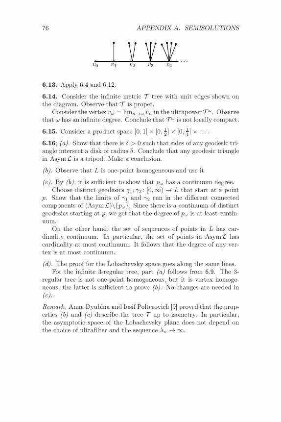
76 APPENDIX A. SEMISOLUTIONS
. . .
v0 v1 v2 v3 v4
6.13. Apply 6.4 and 6.12.
6.14. Consider the infinite metric T tree with unit edges shown onthe diagram. Observe that T is proper.
Consider the vertex vω = limn→ω vn in the ultrapower T ω. Observethat ω has an infinite degree. Conclude that T ω is not locally compact.
6.15. Consider a product space [0, 1]× [0, 12 ]× [0, 14 ]× . . . .
6.16; (a). Show that there is δ > 0 such that sides of any geodesic tri-angle intersect a disk of radius δ. Conclude that any geodesic trianglein AsymL is a tripod. Make a conclusion.
(b). Observe that L is one-point homogeneous and use it.
(c). By (b), it is sufficient to show that pω has a continuum degree.Choose distinct geodesics γ1, γ2 : [0,∞) → L that start at a point
p. Show that the limits of γ1 and γ2 run in the different connectedcomponents of (AsymL)\pω. Since there is a continuum of distinctgeodesics starting at p, we get that the degree of pω is at least contin-uum.
On the other hand, the set of sequences of points in L has car-dinality continuum. In particular, the set of points in AsymL hascardinality at most continuum. It follows that the degree of any ver-tex is at most continuum.
(d). The proof for the Lobachevsky space goes along the same lines.For the infinite 3-regular tree, part (a) follows from 6.9. The 3-
regular tree is not one-point homogeneous, but it is vertex homoge-neous; the latter is sufficient to prove (b). No changes are needed in(c).
Remark. Anna Dyubina and Iosif Polterovich [9] proved that the prop-erties (b) and (c) describe the tree T up to isometry. In particular,the asymptotic space of the Lobachevsky plane does not depend onthe choice of ultrafilter and the sequence λn → ∞.
Index
[∗∗], 9I, 9ε-midpoint, 13λω-asymptotic space, 54λω-tangent space, 54ω-almost all, 49ω-limit, 50ω-limit space, 52ω-small, 491-Lipschitz function, 24
admissible function, 23almost isometry, 39
bounded space, 16
closed ball, 6complete space, 7completion, 7convergence in the sense of Haus-
dorff, 32curve, 10
diameter, 15, 31distance function, 5double, 43doubling, 73doubling measure, 42doubling space, 42
extension, 17extension function, 17extension property, 17extremal function, 23
filter, 50
geodesic, 9
geodesic path, 9gluing, 43
Hausdorff convergence, 35Hausdorff distance, 31homogeneous, 21hyperconvex hull, 30hyperconvex space, 26
induced length metric, 12injective envelope, 29injective space, 25isometry, 8isoperimetric inequality, 34
Lebesgue number, 8length, 10length metric, 12length space, 12Lipschitz function, 32locally compact space, 8
maximal packing, 8metric, 5
∞-metric, 6metric component, 7metric space, 5metric tree, 10midpoint, 13
net, 8nonprincipal ultrafilter, 49norm, 15
one-point extension, 17open ball, 6
partial limit, 33
77
78 INDEX
path, 10pointed convergence, 46proper function, 9proper space, 9pseudometric, 6
rectifiable curve, 10rendezvous value, 61
scaled space, 38, 54selective ultrafilter, 55separable space, 16short map, 16Stone–Cech compactification, 50sup norm, 15
tight span, 30totally bounded space, 8
ultrafilter, 49, 50nonprincipal ultrafilter, 49selective ultrafilter, 55
ultralimit, 50ultrametric space, 25uniformly totally bonded family, 42Urysohn space, 17

Bibliography
[1] S. Alexander, V. Kapovitch, and A. Petrunin. An invitation to Alex-androv geometry: CAT(0) spaces. 2019.
[2] S. Alexander, V. Kapovitch, and A. Petrunin. Alexandrov geometry:preliminary version no. 1. 2019. arXiv: 1903.08539 [math.DG].
[3] N. Aronszajn and P. Panitchpakdi. “Extension of uniformly continu-ous transformations and hyperconvex metric spaces”. Pacific J. Math.6 (1956), 405–439.
[4] E. Bilokopytov. Is it possible to connect every compact set? MathOver-flow. URL:https://mathoverflow.net/q/359390 (version: 2020-05-05).eprint: https://mathoverflow.net/q/359390.
[5] W. Blaschke. Kreis und Kugel. 1916.
[6] M. Bridson and A. Haefliger. Metric spaces of non-positive curvature.Vol. 319. Grundlehren der Mathematischen Wissenschaften [Funda-mental Principles of Mathematical Sciences]. 1999.
[7] D. Burago, Yu. Burago, and S. Ivanov. A course in metric geometry.Vol. 33. Graduate Studies in Mathematics. 2001.
[8] P. Cameron. “The random graph”. The mathematics of Paul Erdos,II. Vol. 14. Algorithms Combin. 1997, 333–351.
[9] A. Dyubina and I. Polterovich. “Explicit constructions of universalR-trees and asymptotic geometry of hyperbolic spaces”. Bull. LondonMath. Soc. 33.6 (2001), 727–734.
[10] M. Frechet. “Sur quelques points du calcul fonctionnel”. Rendicontidel Circolo Matematico di Palermo (1884-1940) 22.1 (1906), 1–72.
[11] Z. Frolık. “Concerning topological convergence of sets”. CzechoslovakMath. J 10(85) (1960), 168–180.
[12] M. Gromov. Metric structures for Riemannian and non-Riemannianspaces. Modern Birkhauser Classics. 2007.
[13] O. Gross. “The rendezvous value of metric space”. Advances in gametheory. Princeton Univ. Press, Princeton, N.J., 1964, 49–53.
[14] F. Hausdorff. Grundzuge der Mengenlehre. 1914.
79
80 BIBLIOGRAPHY
[15] D. Hilbert. „Ueber die gerade Linie als kurzeste Verbindung zweierPunkte.“ Math. Ann. 46 (1895), 91–96.
[16] T. Hu and W. A. Kirk. “Local contractions in metric spaces”. Proc.Amer. Math. Soc. 68.1 (1978), 121–124.
[17] J. R. Isbell. “Six theorems about injective metric spaces”. Comment.Math. Helv. 39 (1964), 65–76.
[18] A. O. Ivanov, N. K. Nikolaeva, and A. A. Tuzhilin. “The Gromov–Hausdorff metric on the space of compact metric spaces is strictlyintrinsic”. Mat. Zametki 100.6 (2016), 947–950.
[19] B. Kleiner and B. Leeb. “Rigidity of quasi-isometries for symmetricspaces and Euclidean buildings”. Inst. Hautes Etudes Sci. Publ. Math.86 (1997), 115–197 (1998).
[20] C. Kuratowski. “Quelques problemes concernant les espaces metriquesnon-separables”. Fundamenta Mathematicae 25.1 (1935), 534–545.
[21] U. Lang, M. Pavon, and R. Zust. “Metric stability of trees and tightspans”. Arch. Math. (Basel) 101.1 (2013), 91–100.
[22] A. Nabutovsky. Linear bounds for constants in Gromov’s systolic in-equality and related results. 2019. arXiv: 1909.12225 [math.MG].
[23] F. Nazarov. Intrinsic metric with no geodesics. MathOverflow. (ver-sion: 2010-02-18). eprint: http://mathoverflow.net/q/15720.
[24] A. Petrunin. Puzzles in geometry that I know and love. 2009. arXiv:0906.0290 [math.HO].
[25] A. Petrunin and S. Stadler. “Metric-minimizing surfaces revisited”.Geom. Topol. 23.6 (2019), 3111–3139.
[26] A. Petrunin and A. Yashinski. “Piecewise isometric mappings”. Alge-bra i Analiz 27.1 (2015), 218–247.
[27] A. Petrunin and S. Zamora Barrera. What is differential geometry:curves and surfaces. 2020. arXiv: 2012.11814 [math.HO].
[28] A. Petrunin. Metric geometry on manifolds: two lectures. 2020. arXiv:2010.10040 [math.DG].
[29] A. Pogorelov. Hilbert’s fourth problem. 1979.
[30] W. Rudin. “Homogeneity problems in the theory of Cech compactifi-cations”. Duke Math. J. 23 (1956), 409–419.
[31] P. Urysohn. “Sur un espace metrique universel”. Bull. Sci. Math51.2 (1927), 43–64. Русский перевод в П.С. Урысон Труды потопологиии другим областям математики, Том II, (1951) 747—777.
[32] J. Vaisala. “A proof of the Mazur–Ulam theorem”. Amer. Math.Monthly 110.7 (2003), 633–635.
[33] R. A. Wijsman. “Convergence of sequences of convex sets, cones andfunctions. II”. Trans. Amer. Math. Soc. 123 (1966), 32–45.