JHEP06(2014)150

Published for SISSA by Springer

Received: September 17, 2013

Revised: April 22, 2014

Accepted: May 15, 2014

Published: June 26, 2014

A novel approach to study atmospheric neutrino

oscillation

Shao-Feng Ge,a Kaoru Hagiwarab and Carsten Rottc

aKEK Theory Center,

Tsukuba, 305-0801, JapanbKEK Theory Center and Sokendai,

Tsukuba, 305-0801, JapancDepartment of Physics, Sungkyunkwan University,

Suwon 440-746, Korea

E-mail: gesf02@gmail.com, kaoru.hagiwara@kek.jp,

carsten.rott@gmail.com

Abstract: We develop a general theoretical framework to analytically disentangle the

contributions of the neutrino mass hierarchy, the atmospheric mixing angle, and the CP

phase, in neutrino oscillations. To illustrate the usefulness of this framework, especially that

it can serve as a complementary tool to neutrino oscillogram in the study of atmospheric

neutrino oscillations, we take PINGU as an example and compute muon- and electron-like

event rates with event cuts on neutrino energy and zenith angle. Under the assumption

of exact measurement of neutrino momentum with a perfect e-µ identification and no

background, we find that the PINGU experiment has the potential of resolving the neutrino

mass hierarchy and the octant degeneracies within 1-year run, while the measurement of the

CP phase is significantly more challenging. Our observation merits a serious study of the

detector capability of estimating the neutrino momentum for both muon- and electron-like

events.

Keywords: Neutrino Physics, Solar and Atmospheric Neutrinos

ArXiv ePrint: 1309.3176

Open Access, c© The Authors.

Article funded by SCOAP3.doi:10.1007/JHEP06(2014)150

JHEP06(2014)150

Contents

1 Introduction 1

2 Disentangling parameters in the propagation basis 3

2.1 Propagation basis 3

2.2 Oscillation probabilities 5

2.3 Simplifications with symmetric matter profile 6

2.4 Expansion of oscillation probabilities with respect to xa = cos 2θa and δm2s 7

3 Event rates at a charge-blind detector 12

4 A simple χ2 analysis 17

4.1 χ2 function 18

4.2 The mass hierarchy 19

4.3 The atmospheric angle and its octant 21

4.3.1 The atmospheric angle 22

4.3.2 Octant sensitivity 23

4.4 Uncertainty of the CP phase 25

5 Conclusions and outlook 27

A Atmospheric neutrino oscillation 28

A.1 Atmospheric neutrino flux, cross sections and effective volume 28

A.2 Earth matter profile 30

A.3 Numerical method for oscillation amplitude matrix S′ in the propagation basis 32

A.4 Normal hierarchy vs. inverted hierarchy 33

1 Introduction

In the last two years, the field of neutrino physics has significantly advanced by constrain-

ing the reactor angle θ13. The T2K experiment [1] was the first to report a hint of nonzero

reactor angle, followed by MINOS [2] and Double CHOOZ [3] which added up to a confi-

dence level above 3 sigma. It was measured accurately by Daya Bay [4] and RENO [5] in

March and April 2012, respectively, reaching 7.7 sigma [6] by the October of the same year.

The relatively large reactor angle opens up opportunities [7] for determining the mass

hierarchy, the octant of the atmospheric mixing angle, and the CP phase. The first could

be achieved with a medium baseline reactor experiment [8–21] and long baseline accel-

erator experiments [22–37, 44] could measure all three of them. Atmospheric neutrino

experiments [38–71] could offer alternative ways to accomplish the same.

– 1 –

JHEP06(2014)150

Recent studies have focused on magnetized detectors, which can distinguish neutri-

nos from antineutrinos [44, 48, 49, 51]. Equipped with this capability, a detector of 50–

100Kton (∼ 103 tons) scale is enough to distinguish the mass hierarchy. Large volume

water-Cherenkov or ice-Cherenkov detectors of tens of Mton (∼ 106 tons) scale could offer

an alternative. DeepCore [52], the existing in-fill to IceCube can reach down to energies

of O(10)GeV and has recently reported the observation of muon neutrino disappearance

oscillations [53] and an electron neutrino flux consistent with expectations [54, 55], demon-

strating the capabilities of an low-energy extension. DeepCore has also some sensitivity

to neutrinos from the MSW resonance region [73–76] around Eν ≈ 5 ∼ 10GeV. It can

however only partially cover it [47, 50] and to really exploit it a lower threshold detector

would be needed.

There has been extensive interest [66–70, 77–81] recently by the IceCube Collaboration

and theoretical community to extend the existing IceCube neutrino telescope [56] with an

in-fill array called PINGU (Precision Icecube Next Generation Upgrade) [57] that could

detect neutrino events of O(1)GeV. Such a detector opens up the opportunity of detecting

more patterns of the atmospheric neutrino oscillation behavior, which is diluted at higher

energy scale, especially due to matter effects [59–65]. A large benefit is the expected high

event statistics at low energies. Event rates of O(100, 000) per year from atmospheric neu-

trinos allow for measurements with small statistical uncertainty. During the preparation of

this draft, a preliminary experimental study [84] appeared. In Europe a similar detector to

PINGU is being considered as part of the Km3NeT project. Our studies can be transferred

to this ORCA (Oscillation Research with Cosmics in the Abyss) [85].

The expectation of a high statistics sample down to 1GeV scale makes determining

the mixing parameters with atmospheric neutrinos very promising [47, 50, 66, 68]. The

paper [66, 68, 69] adopts oscillograms [59–65] to depict the structure of oscillation reso-

nances [61–63, 73–76, 86–95] when atmospheric neutrinos travel through the Earth. The

ability to determine the mass hierarchy, the octant of the atmospheric mixing angle, and

the CP phase is studied. The event numbers and difference between normal hierarchy (NH)

and inverted hierarchy (IH) are shown in oscillograms. In [71], the Bayesian approach is

explored in a generic way while the Toy Monte Carlo based on an extended unbinned

likelihood ratio test statistic is implemented in [72]. When combined with accelerator ex-

periments, the sensitivities on the octant of the atmospheric mixing angle [38, 39, 51, 66, 96]

and the CP phase [97] can be enhanced.

In section 2, we first develop a general framework of decomposing the neutrino os-

cillation probabilities and the event rates in the propagation basis, and apply it to the

symmetric Earth matter profile in order to analytically disentangle the effects of the neu-

trino mass hierarchy, the atmospheric angle, and the CP phase. In section 3, we calculate

and display the event rates that can be observed at PINGU. Based on these results, we

try to establish the potential of atmospheric neutrino measurement at PINGU in section 4,

while its dependence on the input values of the neutrino mass hierarchy, the atmospheric

mixing angle and the CP phase can be fully understood in our decomposition formalism.

Finally, we summarize our conclusions in section 5. For more details about the basic in-

puts, including the atmospheric neutrino fluxes, cross sections, effective fiducial volume of

– 2 –

JHEP06(2014)150

PINGU, and the Earth matter profile, as well as the numerical methods of evaluating the

neutrino oscillation probabilities through Earth, please refer to section A.

2 Disentangling parameters in the propagation basis

We first develop a general framework in the propagation basis [106, 107] for phenomeno-

logical study of neutrino oscillation. It can analytically decompose the contributions of the

neutrino mass hierarchy, the atmospheric mixing angle, and the CP phase. This decom-

position method can serve as a complementary tool to the neutrino oscillogram [59–65] for

the analysis of atmospheric neutrino oscillations, and can apply generally to other types of

neutrino oscillation experiments.

2.1 Propagation basis

In the propagation basis, the atmospheric mixing angle θ23 [106] and the CP phase δ [107]

can be disentangled from the other mixing parameters as well as the Earth matter poten-

tial [108]. This can be seen from the effective Hamiltonian,

H =1

2Eν

U

0

δm2s

δm2a

U † +

a(x)

0

0

, (2.1)

where

a(x) ≡ 2EνV (x) = 2√2EνGFNe(x) , (2.2)

represents the matter effect which is proportional to neutrino energy Eν and the matter

potential V (x). The mass differences are denoted as,

δm2s ≡ m2

2 −m21 , δm2

a ≡ m23 −m2

1 . (2.3)

The lepton-flavor mixing matrix U relates the flavor basis (να = νe, νµ, ντ ) and the mass

eigenstates (mνi = mi, i = 1, 2, 3),

να = Uαiνi , (2.4)

and can be parametrized as U ≡ O23(θa)PδO13(θr)P†δO12(θs),

U ≡

1

ca sa−sa ca

1

1

eiδ

cr sr1

−sr cr

1

1

e−iδ

cs ss−ss cs

1

, (2.5)

where cα ≡ cos θα and sα ≡ sin θα. The solar, the atmospheric, and the reactor mixing

angles are labelled as,

(s, a, r) ≡ (12, 23, 13) , (2.6)

according to how they were measured. For convenience, we denote the three rotation

matrices in (2.5) from the left to the right as O23, O13, and O12 respectively.

– 3 –

JHEP06(2014)150

The 2–3 mixing matrix O23 and the rephasing matrix Pδ can be extracted out as overall

matrices [107, 108],

H =1

2Eν(O23Pδ)

(O13O12)

0

δm2s

δm2a

(O13O12)† +

a(x)

0

0

(O23Pδ)

†. (2.7)

In this way, O23 and Pδ are separated from the neutrino mass hierarchy, which is encoded

in the first term inside the square bracket, as well as the matter effect, represented by

the second term. In other words, the atmospheric mixing angle θa and the CP phase δ

are disentangled from the remaining mixing parameters, analytically. This is a significant

simplification in the analysis of neutrino oscillation, especially the atmospheric neutrino

oscillation that suffers from complicated matter profile, as described in section A.2.

To make it explicit, the original Hamiltonian H can be rotated to the equivalent H′ in

the propagation basis through a similar transformation,

H′ =1

2Eν

(O13O12)

0

δm2s

δm2a

(O13O12)† +

a(x)

0

0

= (O23Pδ)

†H(O23Pδ) .

(2.8)

There are only four mixing parameters involved in H′, the two mass squared differences

δm2s and δm2

a, the solar mixing angle θs, and the reactor mixing angle θr. Correspondingly,

we can define a propagation basis (ν ′i) [106, 107] that is related to the flavor basis (να) and

the mass eigenstates (νi) as follows:

να = [O23(θa)Pδ]αiν′i . (2.9)

The transformed Hamiltonian H′ is the effective Hamiltonian defined in the propagation

basis. Once the neutrino oscillation amplitudes,

S′ij ≡ 〈ν ′j |S′|ν ′i〉 , (2.10)

are calculated with the Hamiltonian H′ in the propagation basis, the oscillation amplitudes

in the flavor basis,

Sαβ ≡ 〈νβ |S|να〉 , (2.11)

are simply obtained by the unitarity transformation,

S = (O23Pδ)S′(O23Pδ)

† ≡ (O23Pδ)

S′11 S′

12 S′13

S′21 S′

22 S′23

S′31 S′

32 S′33

(O23Pδ)†. (2.12)

This makes the formalism much simpler.

We find the propagation basis very useful in the phenomenological study of neutrino

oscillation. It allows us to analytically factor out θa [106] and δ [107] from the numerical

evaluation of the oscillation amplitudes that involves many factors and can be very compli-

cated [108]. The contributions of the still unknown neutrino mass hierarchy, the octant of

– 4 –

JHEP06(2014)150

the atmospheric mixing angle θa, and the CP phase δ are now disentangled from each other.

A general formalism based on this feature can help to reveal the pictures behind neutrino

oscillation phenomena. This is especially important when the three unknown parameters

are under close investigations at current and future neutrino experiments.

2.2 Oscillation probabilities

The oscillation probabilities are measured in the flavor basis. It is necessary to explicitly

express the flavor basis amplitude matrix S in terms of its counterpart S′ in the propagation

basis by the unitary transformation with O23Pδ, namely to expand (2.12). According to

the definition of the mixing matrix in (2.5), O23Pδ can be explicitly written as,

O23Pδ =

1

ca saeiδ

−sa caeiδ

, (O23Pδ)† =

1

ca −sasae

−iδ cae−iδ

. (2.13)

The mixing from the propagation to the flavor basis occurs between the second and the

third indices. We can expect the first element of S′ to be unaffected when (2.13) is combined

with (2.12) [107],

See = S′11 , (2.14a)

Seµ = caS′12 + sae

−iδS′13 , (2.14b)

Sµe = caS′21 + sae

+iδS′31 , (2.14c)

Sµµ = c2aS′22 + casa(e

−iδS′23 + e+iδS′

32) + s2aS′33 . (2.14d)

Note that only the elements among e and µ flavors are shown since they are sufficient to

derive all the flavor basis oscillation probabilities,

Pαβ ≡ P (να → νβ) = |〈νβ|S|να〉|2 = |Sβα|2, (2.15)

from νe and νµ (as well as from νe and νµ, as shown below). Explicitly we find,

Pee ≡ |See|2 = |S′11|2, (2.16a)

Peµ ≡ |Sµe|2 = c2a|S′12|2 + s2a|S′

13|2 + 2casa(cos δR+ sin δI)(S′12S

′∗13) , (2.16b)

Pµe ≡ |Seµ|2 = c2a|S′21|2 + s2a|S′

31|2 + 2casa(cos δR− sin δI)(S′21S

′∗31) , (2.16c)

Pµµ ≡ |Sµµ|2 = c4a|S′22|2 + s4a|S′

33|2 + 2c2as2aR(S

′22S

′∗33)

+c2as2a

[|S′

23|2 + 2(cos 2δR+ sin 2δI)(S′23S

′∗32) + |S′

32|2]

+2casa cos δR[(c2aS

′22 + s2aS

′33)(S

′23 + S′

32)∗]

+2casa sin δI[(c2aS

′22 + s2aS

′33)(S

′32 − S′

23)∗], (2.16d)

where R and I gives the real and imaginary parts, respectively. The dependence on the at-

mospheric mixing angle θa and the CP phase δ can be clearly seen in the above expressions.

The transition probability into ντ are then obtained by unitarity conditions,

Peτ = 1− Pee − Peµ , (2.17a)

Pµτ = 1− Pµe − Pµµ , (2.17b)

– 5 –

JHEP06(2014)150

while we neglect contributions from tiny components of ντ and ντ flux in the atmospheric

neutrinos [102].

The oscillation probabilities for antineutrinos are then obtained simply as,

Pαβ ≡ P (να → νβ) = Pαβ

(a(x) → −a(x), δ → −δ

), (2.18)

by reversing the sign of the matter potential in the Hamiltonian (2.1) and the CP phase δ

in the neutrino mixing matrix (2.5), which is identical to the parametrization adopted in

Review of Particle Physics [109].

2.3 Simplifications with symmetric matter profile

The expressions in (2.16) can be significantly simplified in the approximation of the sym-

metric or reversible matter profile along the baseline, such as those of atmospheric neutrinos

in the earth whose matter profile is approximately spherically symmetric as in PREM [98]

adopted in our study. It has been known that [110] the oscillation amplitude matrix after

experiencing a reversible matter profile is symmetric in the absence of CP violation. This is

indeed the case for the oscillation amplitudes through the Earth in the propagation basis,

giving,

S′ij = S′

ji . (2.19)

Based on the above observation, the atmospheric neutrino oscillation amplitudes (2.14)

can be further simplified,

See = S′11 , (2.20a)

Seµ = caS′12 + sae

−iδS′13 , (2.20b)

Sµe = caS′12 + sae

+iδS′13 , (2.20c)

Sµµ = c2aS′22 + s2aS

′33 + 2casa cos δS

′23 . (2.20d)

As a convention, we adopt those elements S′ij with i ≤ j. It is now manifest that the

flavor oscillation amplitudes Seµ and Sµe differ only by the CP phase and the expression

for Sµµ (2.14d) is greatly simplified in (2.20d). The oscillation probabilities now read,

Pee ≡ |See|2 = |S′11|2, (2.21a)

Peµ ≡ |Sµe|2 = c2a|S′12|2 + s2a|S′

13|2 + 2casa(cos δR+ sin δI)(S′12S

′∗13) , (2.21b)

Pµe ≡ |Seµ|2 = c2a|S′12|2 + s2a|S′

13|2 + 2casa(cos δR− sin δI)(S′12S

′∗13) , (2.21c)

Pµµ ≡ |Sµµ|2 = |c2aS′22 + s2aS

′33|2 + 4c2as

2a cos

2 δ|S′23|2 + 4casa cos δR

[(c2aS

′22 + s2aS

′33)S

′∗23

].

(2.21d)

Throughout our studies in this report we adopt the expression (2.21) for computing

the oscillation probabilities in our numerical calculation, which are exact in the limit of

the symmetric earth matter profile PREM [98] and neglecting the depth of the detector

beneath the earth surface as compared to the baseline lengths. The oscillation probabilities

for antineutrinos Pαβ are then computed as in (2.18).

– 6 –

JHEP06(2014)150

2.4 Expansion of oscillation probabilities with respect to xa = cos 2θa and δm2s

Although the expressions (2.21) for the oscillation probabilities Pαβ , and Pαβ via (2.18),

are simple enough to perform numerical analysis efficiently, we can obtain further insight by

keeping only the leading terms of the following two small parameter of the three neutrino

model,

xa ≡ cos 2θa =√1− sin2 2θa = 0.21+0.06

−0.10 , (2.22a)

δm2s

|δm2a|

= 0.032± 0.002 , (2.22b)

whose numerical values are constrained from the data [109, 111, 112], as summarized below

in (4.3).

First, by expanding ca and sa in terms of xa,

c2a =1

2(1 + xa) , s2a =

1

2(1− xa) , c2as

2a =

1

4(1− x2a) , (2.23)

the oscillation probabilities Pαβ (2.21) are expanded as,

Pee = |S′11|2, (2.24a)

Peµ =1

2

(1−|S′

11|2)+

xa2

(|S′

12|2−|S′13|2)+ (cos δ′R+ sin δ′I)(S′

12S′∗13) +O(x4a) , (2.24b)

Pµe =1

2

(1−|S′

11|2)+

xa2

(|S′

12|2−|S′13|2)+ (cos δ′R− sin δ′I)(S′

12S′∗13) +O(x4a) , (2.24c)

Pµµ =1

4|S′

22 + S′33|2 +

xa2

(|S′

22|2−|S′33|2)+ cos δ′R

[(S′

22 + S′33)S

′∗23

]

+ xa cos δ′R[S′23(S

′22 − S′

33)∗]+

1

4|S′

22 − S′33|2x2a + cos2 δ′|S′

23|2 +O(x4a) . (2.24d)

We can clearly identify the linear terms of xa in Peµ and Pµe, which are identical, and also

in Pµµ. In the above expansion, we keep the terms of order x2a, which turn out to have

significant impacts in the measurement of xa despite the smallness of x2a . 0.05 at 90%

confidence level. Furthermore, we introduce a short-hand notation,

cos δ′ ≡ 2casa cos δ ≈√

1− x2a cos δ , sin δ′ ≡ 2casa sin δ ≈√1− x2a sin δ . (2.25)

in (2.24), without expanding the factor√1− x2a, since all the δ-dependence in the transition

probabilities (2.21) are functions of 2casa cos δ and 2casa sin δ. The uncertainty of the δ-

measurement should be modulated by the factor 1/√1− x2a.

We find it quite useful to express the oscillation probabilities Pαβ in (2.24) and the

corresponding antineutrino oscillation probabilities Pαβ as,

Pαβ ≡ P(0)αβ + P

(1)αβ xa + P

(2)αβ cos δ′ + P

(3)αβ sin δ′ + P

(4)αβ xa cos δ

′ + P(5)αβ x

2a + P

(6)αβ cos2 δ′,

(2.26a)

Pαβ ≡ P(0)αβ + P

(1)αβxa + P

(2)αβ cos δ

′ + P(3)αβ sin δ

′ + P(4)αβxa cos δ

′ + P(5)αβx

2a + P

(6)αβ cos

2 δ′,

(2.26b)

– 7 –

JHEP06(2014)150

where P(0)αβ and P

(0)αβ are the leading terms, while P

(k)αβ and P

(k)αβ with k = 1, · · · , 6 are

the coefficients of corresponding terms linear in xa, cos δ′, sin δ′, xa cos δ

′, x2a, and cos2 δ′,

respectively. The magnitude of these coefficients determines the experimental sensitivity of

measuring the two mixing parameters, xa and δ. The coefficients P(k)αβ of (2.24) are shown

in the following table.

P(k)ee P

(k)eµ P

(k)µe P

(k)µµ

(k = 0) |S′11|2 1

2(1− |S′11|2) 1

2(1− |S′11|2) 1

4 |S′22 + S′

33|2(k = 1) 0 1

2(|S′12|2 − |S′

13|2) 12(|S′

12|2 − |S′13|2) 1

2(|S′22|2 − |S′

33|2)(k = 2) 0 R(S′

12S′∗13) R(S′

12S′∗13) R[S′

23(S′22 + S′

33)∗]

(k = 3) 0 I(S′12S

′∗13) −I(S′

12S′∗13) 0

(k = 4) 0 0 0 R[S′23(S

′22 − S′

33)∗]

(k = 5) 0 0 0 14 |S′

22 − S′33|2

(k = 6) 0 0 0 |S′23|2

(2.27)

It is clearly seen from (2.27) that Pee = P (νe → νe) has no dependence on θa and δ, all

the other oscillation probabilities have terms P(1)αβ linear in xa, the coefficients of cos δ′ are

the same for Peµ and Pµe, those of sin δ′ have the same magnitude but the opposite sign

between Peµ and Pµe, while Pµµ has no dependence on sin δ′. Most of these properties of

the oscillation probabilities are expected from theoretical considerations, while they are

made explicit in (2.26) and (2.27). The corresponding coefficients for the antineutrino

oscillations, P(k)αβ in (2.26b) are obtained from P

(1)αβ in (2.27) as follows:

P(k)αβ = +P

(k)αβ (S

′ij → S

′

ij) for k = 0, 1, 2, 4, 5, 6 , (2.28a)

P(3)αβ = −P

(3)αβ (S

′ij → S

′

ij) , (2.28b)

where S′

ij are the oscillation amplitudes in the propagation basis which are obtained from

S′ij by reversing the sign of the matter potential a(x),

S′

ij = S′ij

(a(x) → −a(x)

). (2.29)

The relation (2.18) between the ν and ν oscillation probabilities, Pαβ and Pαβ , respectively,

is simplified significantly in the propagation basis where the matter dependence and the δ

dependence of the oscillation amplitudes are factorized.

The parameter dependences of the oscillation probabilities Pαβ and Pαβ are further

simplified significantly when we take account of the smallness of the mass squared difference

δm2s as compared to |δm2

a|, (2.22b). We note in the propagation basis Hamiltonian (2.8)

that if we set δm2s ≡ δm2

12 = 0, then the oscillation occurs only between ν ′1 and ν ′3, and

hence the transitions between ν ′1 and ν ′2, and those between ν ′2 and ν ′3 should be suppressed,

|S′12|, |S′

23| = O(δm2

s

δm2a

), (2.30)

– 8 –

JHEP06(2014)150

in the propagation basis. In our numerical study of the atmospheric neutrino oscillations in

the energy range 2GeV < Eν < 20GeV, we find |S′12| < 0.15, and |S′

23| < 0.06. We there-

fore obtain the following approximation by dropping all the terms of order (δm2s/δm

2a)

2,

Pee = |S′11|2, (2.31a)

Peµ =1− xa

2

(1− |S′

11|2)+ (cos δ′R+ sin δ′I)(S′

12S′∗13) +O

(x4a,

(δm2

s

δm2a

)2), (2.31b)

Pµe =1− xa

2

(1− |S′

11|2)+ (cos δ′R− sin δ′I)(S′

12S′∗13) +O

(x4a,

(δm2

s

δm2a

)2), (2.31c)

Pµµ =1

4|S′

22 + S′33|2 +

xa2

(1− |S′

11|2)+

1

4x2a|S′

22 − S′33|2

− cos δ′R(S′12S

′∗13) + xa cos δ

′R[S′23(S

′22 − S′

33)∗]+O

(x4a,

(δm2

s

δm2a

)2), (2.31d)

and (2.27) is further simplified as follows,

P(k)ee P

(k)eµ P

(k)µe P

(k)µµ

(k = 0) |S′11|2 1

2(1− |S′11|2) 1

2(1− |S′11|2) 1

4 |S′22 + S′

33|2(k = 1) 0 −1

2(1− |S′11|2) −1

2(1− |S′11|2) 1

2(1− |S′11|2)

(k = 2) 0 R(S′12S

′∗13) R(S′

12S′∗13) −R(S′

12S′∗13)

(k = 3) 0 I(S′12S

′∗13) −I(S′

12S′∗13) 0

(k = 4) 0 0 0 R[S′23(S

′22 − S′

33)∗]

(k = 5) 0 0 0 14 |S′

22 − S′33|2

(k = 6) 0 0 0 0

(2.32)

In this approximation, there are only 6 independent oscillation factors in the propagation

basis, of which |S′11|2 determines the overall rates P

(0)ee , P

(0)eµ , P

(0)µe , as well as all the coef-

ficients of xa, P(1)eµ , P

(1)µe , and P

(1)µµ . The overall rate P

(0)µµ is governed by |S′

22 + S′23|2. The

coefficients of all the sin δ′ terms are P(3)eµ = −P

(3)µe = I(S′

12S′∗13), and the coefficients of the

cos δ′ terms are P(2)eµ = P

(2)µe = −P

(2)µµ = R(S′

12S′∗13). The remaining cross term xa cos δ

′ is

governed by R[S′23(S

′22 − S′

33)∗] in P

(4)µµ . For the x2a term, its coefficient |S′

22 − S′33|2 is also

independent. The coefficient P(6)µµ of cos2 δ′ in (2.26) and (2.27) is (δm2

s/δm2a)

2 order, and

hence is dropped in (2.31) and (2.32).

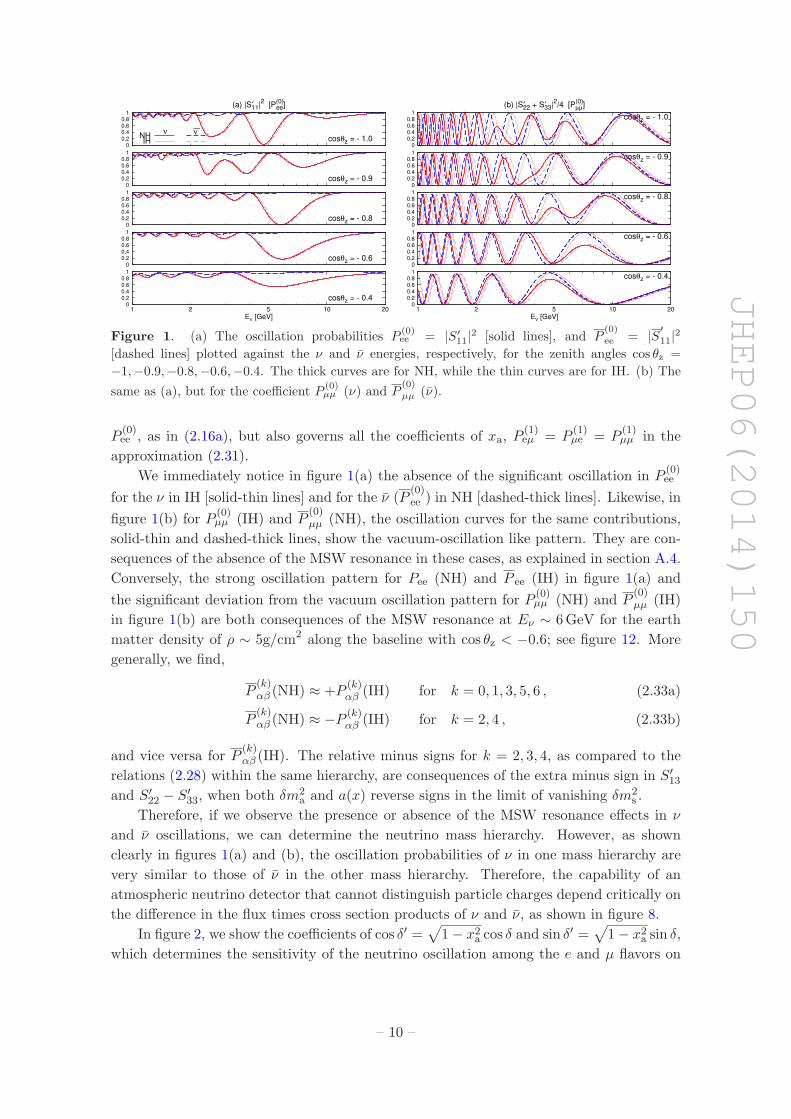
We examine the energy and zenith angle dependence of these 6 oscillation factors

in figure 1 and figure 2. The amplitude matrix elements S′ij in the propagation basis

can be calculated numerically in the way described in section A.3. Shown in figure 1(a)

and (b) are the Eν dependence of the coefficients P(0)ee = |S′

11|2 (P(0)ee = |S′

11|2) and P(0)µµ =

|S′22 + S′

33|2/4 (P(0)µµ = |S′

22 + S′

33|2), respectively, for the baseline along five zenith angles,

cos θz = −1,−0.9,−0.8,−0.6 and −0.4. In each panel, the solid and dashed curves are

for ν and ν oscillations, respectively, shown by the thick lines for NH and by the thin

lines for IH. It should be noted that the coefficient |S′11| in figure 1 not only determines

– 9 –

JHEP06(2014)150

0 0.2 0.4 0.6 0.8

1

cosθz = - 1.0

(a) |S′11|2 [P

(0)ee]

NHIH

ν —ν

0 0.2 0.4 0.6 0.8

1

cosθz = - 0.9

0 0.2 0.4 0.6 0.8

1

cosθz = - 0.8

0 0.2 0.4 0.6 0.8

1

cosθz = - 0.6

0 0.2 0.4 0.6 0.8

1

cosθz = - 0.4

Eν [GeV]1 2 5 10 20

0 0.2 0.4 0.6 0.8

1cosθz = - 1.0

(b) |S′22 + S′33|2/4 [P

(0)µµ]

0 0.2 0.4 0.6 0.8

1cosθz = - 0.9

0 0.2 0.4 0.6 0.8

1cosθz = - 0.8

0 0.2 0.4 0.6 0.8

1cosθz = - 0.6

0 0.2 0.4 0.6 0.8

1cosθz = - 0.4

Eν [GeV]1 2 5 10 20

Figure 1. (a) The oscillation probabilities P(0)ee = |S′

11|2 [solid lines], and P(0)

ee = |S′

11|2[dashed lines] plotted against the ν and ν energies, respectively, for the zenith angles cos θz =

−1,−0.9,−0.8,−0.6,−0.4. The thick curves are for NH, while the thin curves are for IH. (b) The

same as (a), but for the coefficient P(0)µµ (ν) and P

(0)

µµ (ν).

P(0)ee , as in (2.16a), but also governs all the coefficients of xa, P

(1)eµ = P

(1)µe = P

(1)µµ in the

approximation (2.31).

We immediately notice in figure 1(a) the absence of the significant oscillation in P(0)ee

for the ν in IH [solid-thin lines] and for the ν (P(0)ee ) in NH [dashed-thick lines]. Likewise, in

figure 1(b) for P(0)µµ (IH) and P

(0)µµ (NH), the oscillation curves for the same contributions,

solid-thin and dashed-thick lines, show the vacuum-oscillation like pattern. They are con-

sequences of the absence of the MSW resonance in these cases, as explained in section A.4.

Conversely, the strong oscillation pattern for Pee (NH) and P ee (IH) in figure 1(a) and

the significant deviation from the vacuum oscillation pattern for P(0)µµ (NH) and P

(0)µµ (IH)

in figure 1(b) are both consequences of the MSW resonance at Eν ∼ 6GeV for the earth

matter density of ρ ∼ 5g/cm2 along the baseline with cos θz < −0.6; see figure 12. More

generally, we find,

P(k)αβ (NH) ≈ +P

(k)αβ (IH) for k = 0, 1, 3, 5, 6 , (2.33a)

P(k)αβ (NH) ≈ −P

(k)αβ (IH) for k = 2, 4 , (2.33b)

and vice versa for P(k)αβ (IH). The relative minus signs for k = 2, 3, 4, as compared to the

relations (2.28) within the same hierarchy, are consequences of the extra minus sign in S′13

and S′22 − S′

33, when both δm2a and a(x) reverse signs in the limit of vanishing δm2

s .

Therefore, if we observe the presence or absence of the MSW resonance effects in ν

and ν oscillations, we can determine the neutrino mass hierarchy. However, as shown

clearly in figures 1(a) and (b), the oscillation probabilities of ν in one mass hierarchy are

very similar to those of ν in the other mass hierarchy. Therefore, the capability of an

atmospheric neutrino detector that cannot distinguish particle charges depend critically on

the difference in the flux times cross section products of ν and ν, as shown in figure 8.

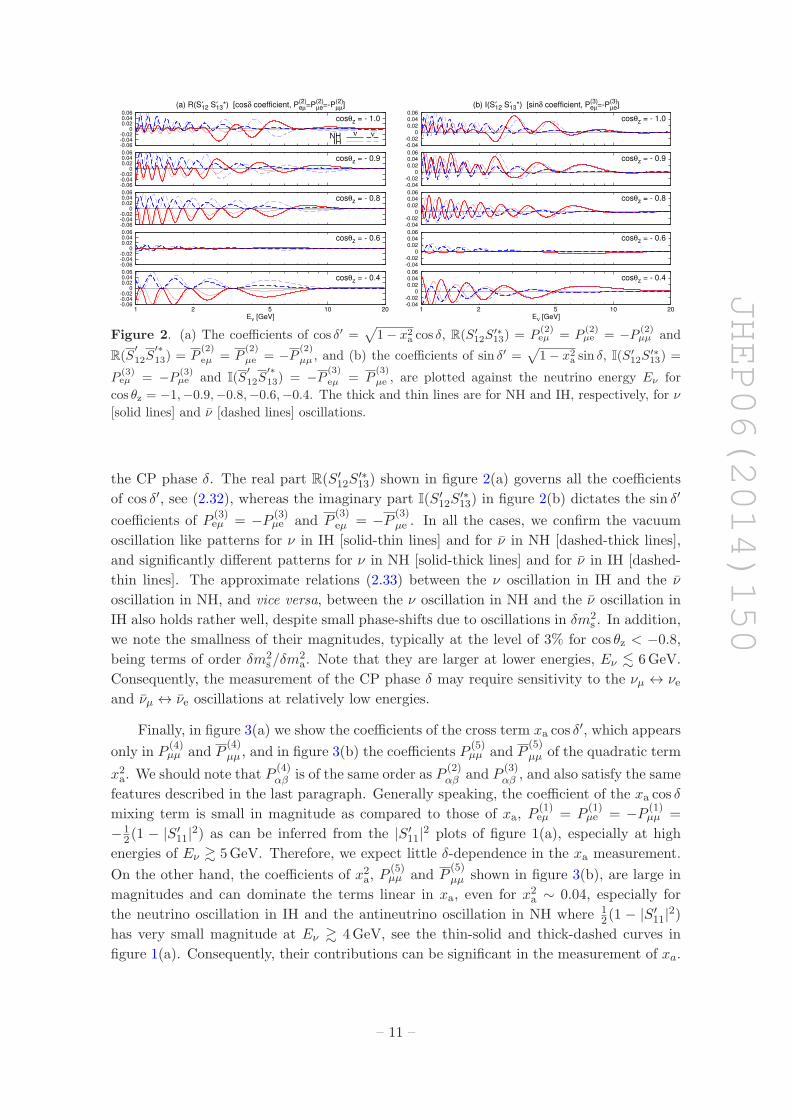
In figure 2, we show the coefficients of cos δ′ =√1− x2a cos δ and sin δ′ =

√1− x2a sin δ,

which determines the sensitivity of the neutrino oscillation among the e and µ flavors on

– 10 –

JHEP06(2014)150

-0.06-0.04-0.02

0 0.02 0.04 0.06

cosθz = - 1.0

(a) R(S′12 S′13*) [cosδ coefficient, P(2)eµ=P

(2)µe=-P

(2)µµ]

NHIH

ν —ν

-0.06-0.04-0.02

0 0.02 0.04 0.06

cosθz = - 0.9

-0.06-0.04-0.02

0 0.02 0.04 0.06

cosθz = - 0.8

-0.06-0.04-0.02

0 0.02 0.04 0.06

cosθz = - 0.6

-0.06-0.04-0.02

0 0.02 0.04 0.06

cosθz = - 0.4

Eν [GeV]1 2 5 10 20

-0.04-0.02

0 0.02 0.04 0.06

cosθz = - 1.0

(b) I(S′12 S′13*) [sinδ coefficient, P(3)eµ=-P

(3)µe]

-0.04-0.02

0 0.02 0.04 0.06

cosθz = - 0.9

-0.04-0.02

0 0.02 0.04 0.06

cosθz = - 0.8

-0.04-0.02

0 0.02 0.04 0.06

cosθz = - 0.6

-0.04-0.02

0 0.02 0.04 0.06

cosθz = - 0.4

Eν [GeV]1 2 5 10 20

Figure 2. (a) The coefficients of cos δ′ =√1− x2

a cos δ, R(S′

12S′∗

13) = P(2)eµ = P

(2)µe = −P

(2)µµ and

R(S′

12S′∗

13) = P(2)

eµ = P(2)

µe = −P(2)

µµ , and (b) the coefficients of sin δ′ =√1− x2

a sin δ, I(S′

12S′∗

13) =

P(3)eµ = −P

(3)µe and I(S

′

12S′∗

13) = −P(3)

eµ = P(3)

µe , are plotted against the neutrino energy Eν for

cos θz = −1,−0.9,−0.8,−0.6,−0.4. The thick and thin lines are for NH and IH, respectively, for ν

[solid lines] and ν [dashed lines] oscillations.

the CP phase δ. The real part R(S′12S

′∗13) shown in figure 2(a) governs all the coefficients

of cos δ′, see (2.32), whereas the imaginary part I(S′12S

′∗13) in figure 2(b) dictates the sin δ′

coefficients of P(3)eµ = −P

(3)µe and P

(3)eµ = −P

(3)µe . In all the cases, we confirm the vacuum

oscillation like patterns for ν in IH [solid-thin lines] and for ν in NH [dashed-thick lines],

and significantly different patterns for ν in NH [solid-thick lines] and for ν in IH [dashed-

thin lines]. The approximate relations (2.33) between the ν oscillation in IH and the ν

oscillation in NH, and vice versa, between the ν oscillation in NH and the ν oscillation in

IH also holds rather well, despite small phase-shifts due to oscillations in δm2s . In addition,

we note the smallness of their magnitudes, typically at the level of 3% for cos θz < −0.8,

being terms of order δm2s/δm

2a. Note that they are larger at lower energies, Eν . 6GeV.

Consequently, the measurement of the CP phase δ may require sensitivity to the νµ ↔ νeand νµ ↔ νe oscillations at relatively low energies.

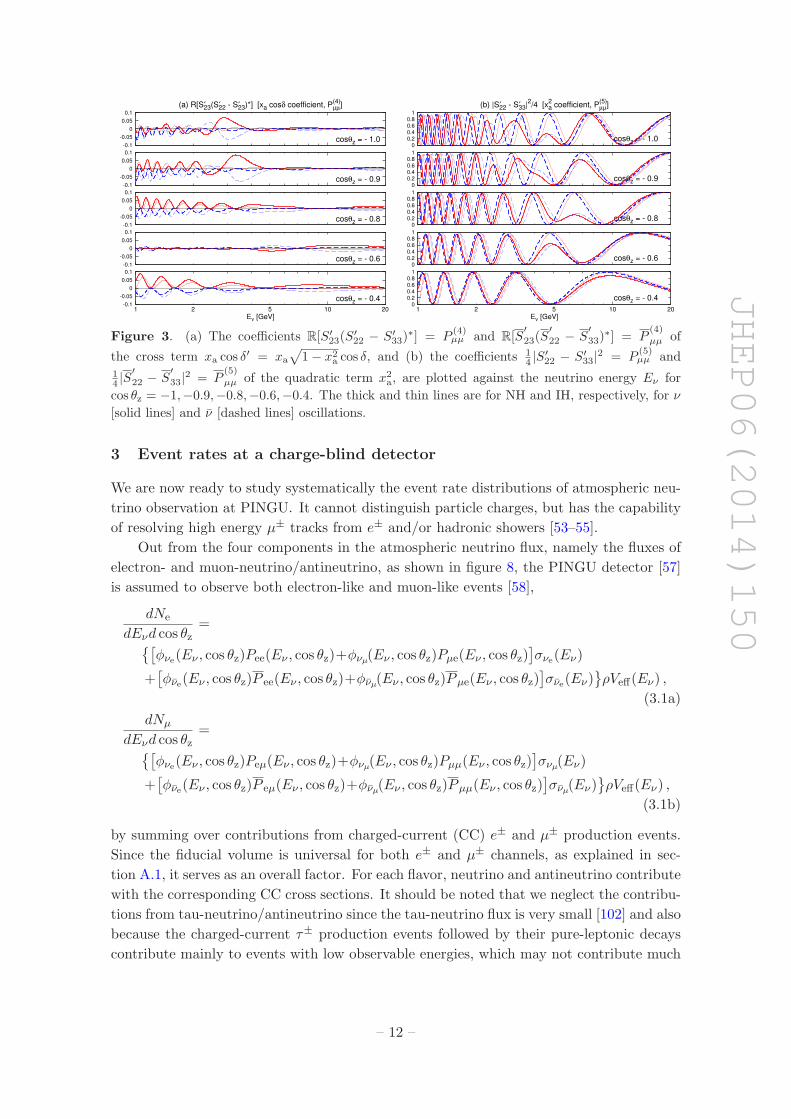
Finally, in figure 3(a) we show the coefficients of the cross term xa cos δ′, which appears

only in P(4)µµ and P

(4)µµ , and in figure 3(b) the coefficients P

(5)µµ and P

(5)µµ of the quadratic term

x2a. We should note that P(4)αβ is of the same order as P

(2)αβ and P

(3)αβ , and also satisfy the same

features described in the last paragraph. Generally speaking, the coefficient of the xa cos δ

mixing term is small in magnitude as compared to those of xa, P(1)eµ = P

(1)µe = −P

(1)µµ =

−12(1 − |S′

11|2) as can be inferred from the |S′11|2 plots of figure 1(a), especially at high

energies of Eν & 5GeV. Therefore, we expect little δ-dependence in the xa measurement.

On the other hand, the coefficients of x2a, P(5)µµ and P

(5)µµ shown in figure 3(b), are large in

magnitudes and can dominate the terms linear in xa, even for x2a ∼ 0.04, especially for

the neutrino oscillation in IH and the antineutrino oscillation in NH where 12(1 − |S′

11|2)has very small magnitude at Eν & 4GeV, see the thin-solid and thick-dashed curves in

figure 1(a). Consequently, their contributions can be significant in the measurement of xa.

– 11 –

JHEP06(2014)150

-0.1

-0.05

0

0.05

0.1

cosθz = - 1.0

(a) R[S′23(S′22 - S′23)*] [xa cosδ coefficient, P(4)µµ]

-0.1

-0.05

0

0.05

0.1

cosθz = - 0.9

-0.1

-0.05

0

0.05

0.1

cosθz = - 0.8

-0.1

-0.05

0

0.05

0.1

cosθz = - 0.6

-0.1

-0.05

0

0.05

0.1

cosθz = - 0.4

Eν [GeV]1 2 5 10 20

0 0.2 0.4 0.6 0.8

1

cosθz = - 1.0

(b) |S′22 - S′33|2/4 [x

2a coefficient, P

(5)µµ]

0 0.2 0.4 0.6 0.8

1

cosθz = - 0.9

0 0.2 0.4 0.6 0.8

1

cosθz = - 0.8

0 0.2 0.4 0.6 0.8

1

cosθz = - 0.6

0 0.2 0.4 0.6 0.8

1

cosθz = - 0.4

Eν [GeV]1 2 5 10 20

Figure 3. (a) The coefficients R[S′

23(S′

22 − S′

33)∗] = P

(4)µµ and R[S

′

23(S′

22 − S′

33)∗] = P

(4)

µµ of

the cross term xa cos δ′ = xa

√1− x2

a cos δ, and (b) the coefficients 14 |S′

22 − S′

33|2 = P(5)µµ and

14 |S

′

22 − S′

33|2 = P(5)

µµ of the quadratic term x2a, are plotted against the neutrino energy Eν for

cos θz = −1,−0.9,−0.8,−0.6,−0.4. The thick and thin lines are for NH and IH, respectively, for ν

[solid lines] and ν [dashed lines] oscillations.

3 Event rates at a charge-blind detector

We are now ready to study systematically the event rate distributions of atmospheric neu-

trino observation at PINGU. It cannot distinguish particle charges, but has the capability

of resolving high energy µ± tracks from e± and/or hadronic showers [53–55].

Out from the four components in the atmospheric neutrino flux, namely the fluxes of

electron- and muon-neutrino/antineutrino, as shown in figure 8, the PINGU detector [57]

is assumed to observe both electron-like and muon-like events [58],

dNe

dEνd cos θz=

{[φνe(Eν , cos θz)Pee(Eν , cos θz)+φνµ(Eν , cos θz)Pµe(Eν , cos θz)

]σνe(Eν)

+[φνe(Eν , cos θz)P ee(Eν , cos θz)+φνµ(Eν , cos θz)Pµe(Eν , cos θz)

]σνe(Eν)

}ρVeff(Eν) ,

(3.1a)

dNµ

dEνd cos θz=

{[φνe(Eν , cos θz)Peµ(Eν , cos θz)+φνµ(Eν , cos θz)Pµµ(Eν , cos θz)

]σνµ(Eν)

+[φνe(Eν , cos θz)P eµ(Eν , cos θz)+φνµ(Eν , cos θz)Pµµ(Eν , cos θz)

]σνµ(Eν)

}ρVeff(Eν) ,

(3.1b)

by summing over contributions from charged-current (CC) e± and µ± production events.

Since the fiducial volume is universal for both e± and µ± channels, as explained in sec-

tion A.1, it serves as an overall factor. For each flavor, neutrino and antineutrino contribute

with the corresponding CC cross sections. It should be noted that we neglect the contribu-

tions from tau-neutrino/antineutrino since the tau-neutrino flux is very small [102] and also

because the charged-current τ± production events followed by their pure-leptonic decays

contribute mainly to events with low observable energies, which may not contribute much

– 12 –

JHEP06(2014)150

due to the smaller fiducial volume. In addition, the tau neutrino cross section is small

compared to the CC electron and muon neutrino cross sections [103]. Contributions from

the charged-current τ± production events as well as neutral-current events will be studied

elsewhere.

Since the number of signal events depends on the oscillation probabilities linearly, which

have been decomposed into six terms in (2.26), the event rates can also be decomposed

accordingly,

dNα

dEνd cos θz≡ N (0)

α +N (1)α xa+N (2)

α cos δ′+N (3)α sin δ′+N (4)

α xa cos δ′+N (5)

α x2a +N (6)α cos2 δ′.

(3.2)

By combining with the explicit expressions of the decomposed oscillation probabilities

in (2.27), the coefficients for electron-like event number rates are,

N (0)e =

{[φνe |S′

11|2 + φνµ

1

2

(1− |S′

11|2)]σνe +

[φνe |S

′

11|2 + φνµ

1

2

(1− |S′

11|2)]σνe

}ρVeff ,

(3.3a)

N (1)e =

{− φνµ

1

2

(1− |S′

11|2)σνe − φνµ

1

2

(1− |S′

11|2)σνe

}ρVeff , (3.3b)

N (2)e =

[+ φνµR(S

′12S

′∗13)σνe+ φνµR

(S′

12S′∗

13

)σνe]ρVeff , (3.3c)

N (3)e =

[− φνµ I(S

′12S

′∗13)σνe + φνµ I

(S′

12S′∗

13

)σνe]ρVeff , (3.3d)

N (4)e = N (5)

e = N (6)e = 0 . (3.3e)

For brevity, the arguments Eν and cos θz have been omitted. Note that there is no term

with xa cos δ′, x2a or cos2 δ′ dependence for electron-like events since P

(4)ee = P

(4)µe = P

(5)ee =

P(5)µe = P

(6)ee = P

(6)µe = 0 and the same for antineutrinos as shown in (2.27) and (2.32). In

other words, the atmospheric angle θa and the CP phase δ are naturally disentangled in

the electron-like events, which depend on θa through N(1)e while the dependence on the CP

phase δ comes from N(2)e and N

(3)e .

For the muon-like events, we find,

N (0)µ =

{[φνe

1

2

(1− |S′

11|2)+ φνµ

1

4|S′

22 + S′33|2]σνµ

+

[φνe

1

2

(1− |S′

11|2)+ φνµ

1

4|S′

22 + S′

33|2]σνµ

}ρVeff , (3.4a)

N (1)µ =

{(φνµ − φνe)

1

2

(1− |S′

11|2)σνµ + (φνµ − φνe)

1

2

(1− |S′

11|2)σνµ

}ρVeff , (3.4b)

N (2)µ =

{(φνe − φνµ)R(S

′12S

′∗13)σνµ + (φνe − φνµ)R

(S′

12S′∗

13

)σνµ}ρVeff , (3.4c)

N (3)µ =

{φνeI(S

′12S

′∗13)σνµ − φνeI

(S′

12S′∗

13

)σνµ}ρVeff , (3.4d)

N (4)µ =

{φνµR

[S′23(S

′22 − S′

33)∗]σνµ + φνµR

[S′

23

(S′

22 − S′

33

)∗]σνµ}ρVeff , (3.4e)

N (5)µ =

{φνµ

1

4|S′

22 − S′33|2σνµ + φνµ

1

4|S′

22 − S′

33|2σνµ}ρVeff , (3.4f)

N (6)µ =

{φνµ |S′

23|2σνµ + φνµ |S′

23|2σνµ}ρVeff . (3.4g)

– 13 –

JHEP06(2014)150

0 2000 4000 6000 8000

cosθz = - 1.0

(a) muon-like events [GeV-1

yr-1

]

NHIH

N(0) N

(1)

0 2000 4000 6000 8000

cosθz = - 0.9

0 2000 4000 6000 8000

cosθz = - 0.8

0 2000 4000 6000 8000

cosθz = - 0.6

0 2000 4000 6000 8000

cosθz = - 0.4

Eν [GeV]1 2 5 10 20

-1000 0

1000 2000 3000

cosθz = - 1.0

(b) electron-like events [GeV-1

yr-1

]

-1000 0

1000 2000 3000

cosθz = - 0.9

-1000 0

1000 2000 3000

cosθz = - 0.8

-1000 0

1000 2000 3000

cosθz = - 0.6

-1000 0

1000 2000 3000 4000

cosθz = - 0.4

Eν [GeV]1 2 5 10 20

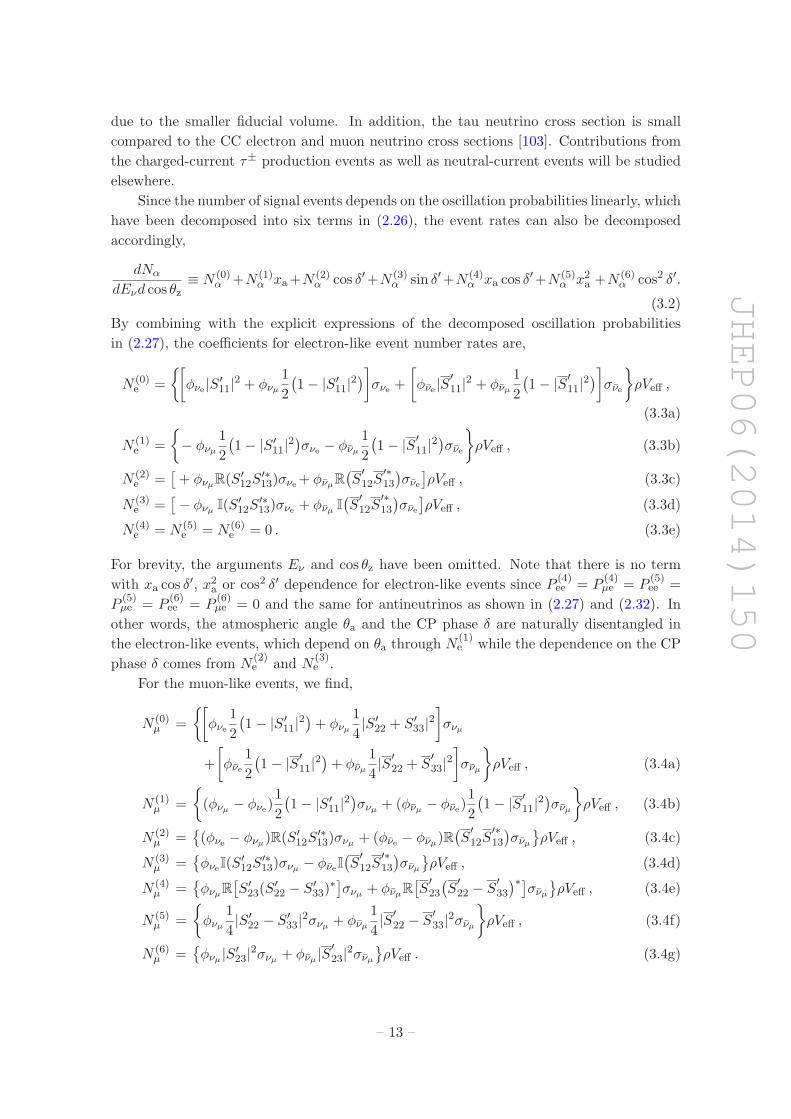
Figure 4. The overall rates N(0)α [red-thick lines] and the coefficients N

(1)α of xa [blue-thin lines]

are plotted against Eν at cos θz = −1,−0.9,−0.8,−0.6,−0.4, for the muon-like [α = µ] events (a)

and the electron-like [α = e] events (b). The solid curves are for NH, while the dashed curves are

for IH. The vertical scale gives the number of events per GeV in one year.

Note that for muon-like events, the crossing term xa cos δ′ has nonvanishing coefficient

N(4)µ . Consequently, with muon-like events included, we should observe some correlation

between the measurements of the atmospheric mixing angle xa and the CP phase δ, as

will be described in section 4. In addition, a nonzero N(6)µ , which is one further order of

magnitude smaller than N(4)µ , is kept according to (2.27) just to show its magnitude.

By combining everything together, the atmospheric neutrino flux, cross section and

effective fiducial volume of figure 8 in section A.1, the earth matter profile in section A.2,

and the oscillation probabilities discussed in section 2 together with the numerical method

described in section A.3, the energy and the zenith angle dependences of the coefficients for

muon- and electron-like event rates are shown in figure 4, figure 5, figure 6, and figure 7.

Note the different scales of the plots, which are adjusted to show the structure of the

coefficients.

In figure 4, we show the overall rates N(0)α in red-thick lines and the coefficients N

(1)α of

xa in blue-thin lines, as functions of Eν at several cos θz, for muon-like [α = µ] events (a)

and for electron-like [α = e] events (b). The solid curves are for the normal hierarchy

(NH), while the dashed curves are for the inverted hierarchy (IH). The muon-like event

rates N(0)µ in the left panel figure 4(a) show significant oscillatory behavior for both NH

(thick-solid lines) and IH (thick-dashed lines). However, the huge hierarchy dependences in

the νµ → νµ oscillation (MSW [73–76] resonance only for NH) and in the νµ → νµ oscillation

(MSW resonance only for IH) as shown in figure 1(b) diminish significantly because of the

cancellation between the νµ and νµ contributions. Because the flux times cross section for

νµ is a factor of about three larger than that for νµ as shown in figure 8(b), the hierarchy

dependence of the νµ → νµ oscillation survives, resulting in the smaller rate for IH at the

MSW resonant energy of ∼ 6GeV at cos θz−0.8. Especially at cos θz . −0.9, shown in the

top two panels of figure 4(a), the nearly maximal resonant oscillation of νµ → νµ for NH at

Eν ∼ 4GeV shown by the thick-red curves in the top two panels of figure 1(b) gives rise to

the significant difference in the muon-like event rate in the 3 ∼ 5GeV region due to the so-

– 14 –

JHEP06(2014)150

-100

-50

0

50

100

cosθz = - 1.0

(a) muon-like events, NH [GeV-1

yr-1

]

N(2)

[cosδ]N

(3) [ sinδ]

-100

-50

0

50

100

cosθz = - 0.9

-100

-50

0

50

100

cosθz = - 0.8

-20

-10

0

10

cosθz = - 0.6

-150-100

-50 0

50 100 150

cosθz = - 0.4

Eν [GeV]1 2 5 10 20

-200

-100

0

100

200

cosθz = - 1.0

(b) electron-like events, NH [GeV-1

yr-1

]

-200

-100

0

100

200

cosθz = - 0.9

-200

-100

0

100

cosθz = - 0.8

-25

0

25

50

cosθz = - 0.6

-300

-150

0

150

300

cosθz = - 0.4

Eν [GeV]1 2 5 10 20

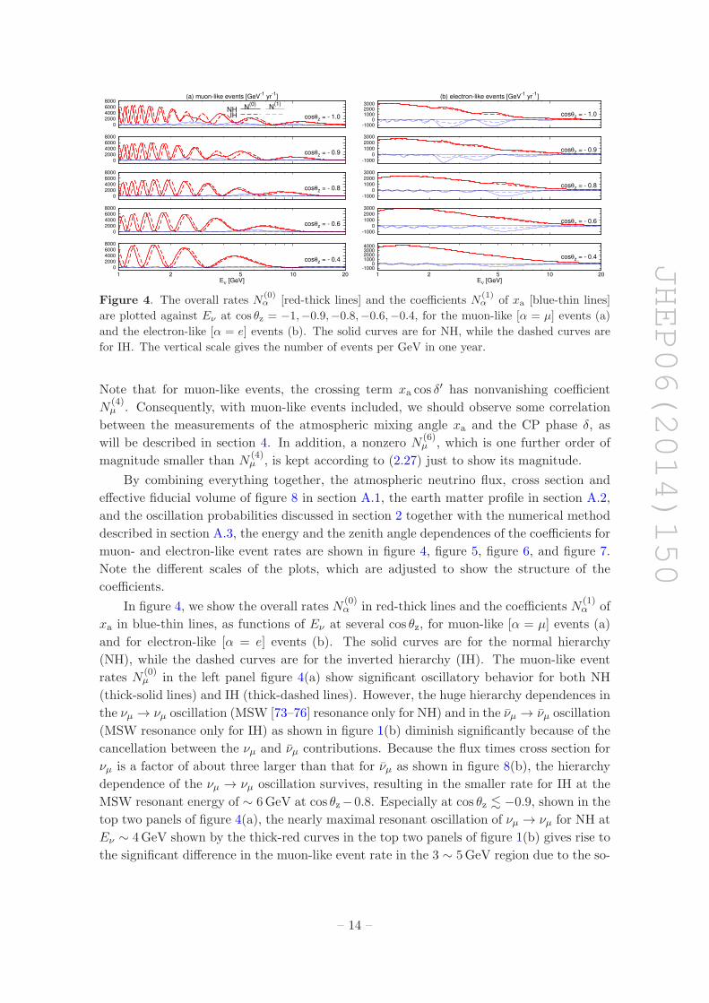
Figure 5. The coefficients N(2)α of cos δ′ =

√1− x2

a cos δ [red-solid lines] and N(3)α of sin δ′ =√

1− x2a sin δ [blue-dashed lines] for the muon-like (α = µ) events (a) and electron-like events (b)

for NH.

called parametric resonance [61–63, 86–95]. Because of the large event numbers, there is a

possibility that these differences can be identified in experiments and that the neutrino mass

hierarchy is determined. We note, however, that the finite energy and angular resolution

of real experiments may make it difficult to identify differences which depend strongly on

the energy, such as those in the oscillation phase observed at Eν . 4GeV at all cos θz. On

the other hand, the hierarchy dependence of the electron-like event rate N(0)e , shown also

by thick-red lines in figure 4(b), has little dependence on cos θz and does not oscillate in

Eν . Although both the overall rate and the difference is small, the event is consistently

higher for NH than IH in the broad energy range of 2 ∼ 10GeV, reflecting the MSW and

parametric enhancements of the νµ → νe oscillation, P(0)µe = 1

2(1−|S′11|2), for NH; see (2.32)

and figure 1(a). Such moderate Eν and cos θz dependences of the electron-like event rate

on the mass hierarchy may allow actual experiments to identify the difference.

Let us now examine the coefficients N(1)µ and N

(1)e of xa, which are shown by thin-blue

lines in figure 4(a) and (b), respectively, also in solid for NH and in dashed for IH. Note

that N(1)µ is positive definite while N

(1)e tends to be negative at high energies (Eν & 2GeV).

The coefficients N(1)µ and N

(1)e are both proportional to 1

2(1− |S′11|2) in the approximation

of (2.32), and hence the energy-angular dependences are mild especially at high energy

region of 4 ∼ 10GeV, just like the electron-like event rate N(0)e . This will help experiments

to measure xa. Because of the positive sign of N(1)µ , the mass hierarchy determination

by using only the muon-like events should be easier for xa < 0 (sin2 θa < 0.5) than for

xa > 0 (sin2 θa > 0.5). The trend can be reversed when the electron-like events are also

included because N(1)e has negative sign and has relatively larger magnitude. Likewise, xa

will be measured more accurately for NH than for IH when only the muon-like events are

studied, whereas the measurement for IH can be significantly improved by including the

electron-like events in the analysis.

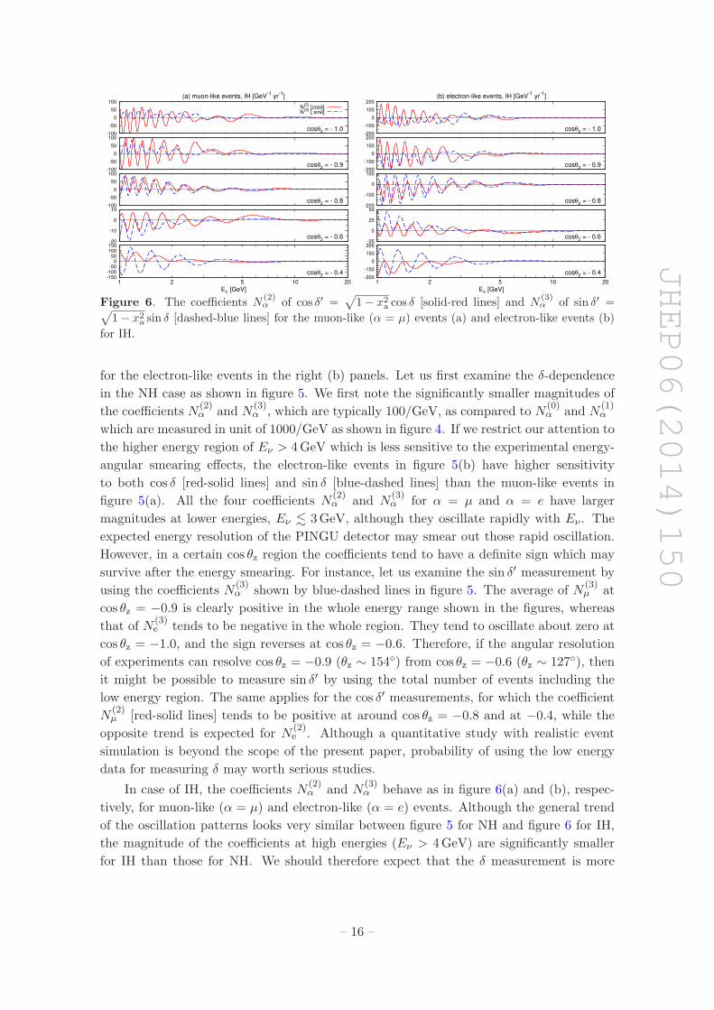
The dependence on the CP phase δ is shown in figure 5 and figure 6, respectively, for

NH and IH. In both figures, the N(2)α [red-solid lines] coefficient of

√1− x2a cos δ and N

(3)α

[blue-dashed lines] of√1− x2a sin δ are shown for the muon-like events in the left (a) and

– 15 –

JHEP06(2014)150

-100

-50

0

50

100

cosθz = - 1.0

(a) muon-like events, IH [GeV-1

yr-1

]

N(2)

[cosδ]N

(3) [ sinδ]

-100

-50

0

50

100

cosθz = - 0.9

-100

-50

0

50

100

cosθz = - 0.8

-20

-10

0

10

cosθz = - 0.6

-150-100

-50 0

50 100 150

cosθz = - 0.4

Eν [GeV]1 2 5 10 20

-200

-100

0

100

200

cosθz = - 1.0

(b) electron-like events, IH [GeV-1

yr-1

]

-200

-100

0

100

200

cosθz = - 0.9

-200

-100

0

100

cosθz = - 0.8

-25

0

25

50

cosθz = - 0.6

-300

-150

0

150

300

cosθz = - 0.4

Eν [GeV]1 2 5 10 20

Figure 6. The coefficients N(2)α of cos δ′ =

√1− x2

a cos δ [solid-red lines] and N(3)α of sin δ′ =√

1− x2a sin δ [dashed-blue lines] for the muon-like (α = µ) events (a) and electron-like events (b)

for IH.

for the electron-like events in the right (b) panels. Let us first examine the δ-dependence

in the NH case as shown in figure 5. We first note the significantly smaller magnitudes of

the coefficients N(2)α and N

(3)α , which are typically 100/GeV, as compared to N

(0)α and N

(1)α

which are measured in unit of 1000/GeV as shown in figure 4. If we restrict our attention to

the higher energy region of Eν > 4GeV which is less sensitive to the experimental energy-

angular smearing effects, the electron-like events in figure 5(b) have higher sensitivity

to both cos δ [red-solid lines] and sin δ [blue-dashed lines] than the muon-like events in

figure 5(a). All the four coefficients N(2)α and N

(3)α for α = µ and α = e have larger

magnitudes at lower energies, Eν . 3GeV, although they oscillate rapidly with Eν . The

expected energy resolution of the PINGU detector may smear out those rapid oscillation.

However, in a certain cos θz region the coefficients tend to have a definite sign which may

survive after the energy smearing. For instance, let us examine the sin δ′ measurement by

using the coefficients N(3)α shown by blue-dashed lines in figure 5. The average of N

(3)µ at

cos θz = −0.9 is clearly positive in the whole energy range shown in the figures, whereas

that of N(3)e tends to be negative in the whole region. They tend to oscillate about zero at

cos θz = −1.0, and the sign reverses at cos θz = −0.6. Therefore, if the angular resolution

of experiments can resolve cos θz = −0.9 (θz ∼ 154◦) from cos θz = −0.6 (θz ∼ 127◦), then

it might be possible to measure sin δ′ by using the total number of events including the

low energy region. The same applies for the cos δ′ measurements, for which the coefficient

N(2)µ [red-solid lines] tends to be positive at around cos θz = −0.8 and at −0.4, while the

opposite trend is expected for N(2)e . Although a quantitative study with realistic event

simulation is beyond the scope of the present paper, probability of using the low energy

data for measuring δ may worth serious studies.

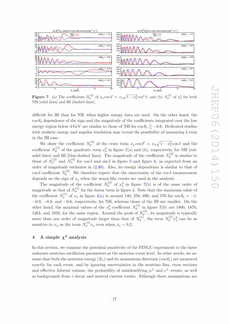
In case of IH, the coefficients N(2)α and N

(3)α behave as in figure 6(a) and (b), respec-

tively, for muon-like (α = µ) and electron-like (α = e) events. Although the general trend

of the oscillation patterns looks very similar between figure 5 for NH and figure 6 for IH,

the magnitude of the coefficients at high energies (Eν > 4GeV) are significantly smaller

for IH than those for NH. We should therefore expect that the δ measurement is more

– 16 –

JHEP06(2014)150

-200-100

0 100 200 300

cosθz = - 1.0

(a) N(4)µ [xa cosδ] for muon-like events [GeV

-1 yr

-1]

[NH][IH]

-200-100

0 100 200 300

cosθz = - 0.9

-50 0

50 100 150 200 250

cosθz = - 0.8

-50-25

0 25 50

cosθz = - 0.6

-100 0

100 200 300 400

cosθz = - 0.4

Eν [GeV]1 2 5 10 20

0 2000 4000 6000 8000

cosθz = - 1.0

(b) N(5)µ [x

2a] for muon-like events [GeV

-1 yr

-1]

[NH][IH]

0 2000 4000 6000 8000

cosθz = - 0.9

0 2000 4000 6000 8000

cosθz = - 0.8

0 2000 4000 6000 8000

cosθz = - 0.6

0 2000 4000 6000 8000

cosθz = - 0.4

Eν [GeV]1 2 5 10 20

Figure 7. (a) The coefficients N(4)µ of xa cos δ

′ = xa

√1− x2

a cos2 δ, and (b) N

(5)µ of x2

a for both

NH [solid lines] and IH [dashed lines].

difficult for IH than for NH, when higher energy data are used. On the other hand, the

cos θz dependence of the sign and the magnitude of the coefficients integrated over the low

energy region below 4GeV are similar to those of NH for cos θz & −0.6. Dedicated studies

with realistic energy and angular resolution may reveal the possibility of measuring δ even

in the IH case.

We show the coefficient N(4)µ of the cross term xa cos δ

′ = xa√1− x2a cos δ and the

coefficient N(5)µ of the quadratic term x2a in figure 7(a) and (b), respectively, for NH [red-

solid lines] and IH [blue-dashed lines]. The magnitude of the coefficient N(4)µ is similar to

those of N(2)α and N

(3)α for cos δ and sin δ in figure 5 and figure 6, as expected from an

order of magnitude estimates in (2.30). Also, its energy dependence is similar to that of

cos δ coefficient N(2)µ . We therefore expect that the uncertainty of the cos δ measurement

depends on the sign of xa when the muon-like events are used in the analysis.

The magnitude of the coefficient N(5)µ of x2a in figure 7(b) is of the same order of

magnitude as that of N(1)α for the linear term in figure 4. Note that the maximum value of

the coefficient N(1)µ of xa in figure 4(a) is around 140, 250, 690, and 570 for cos θz = −1,

−0.9, −0.8, and −0.6, respectively, for NH, whereas those of the IH are smaller. On the

other hand, the maximal values of the x2a coefficient N(5)µ in figure 7(b) are 1800, 1870,

1264, and 1050, for the same region. Around the peak of N(5)µ , its magnitude is typically

more than one order of magnitude larger than that of N(1)µ , the term N

(5)µ x2a can be as

sensitive to xa as the term N(1)µ xa even when xa ∼ 0.2.

4 A simple χ2 analysis

In this section, we examine the potential sensitivity of the PINGU experiment to the three

unknown neutrino oscillation parameters at the neutrino event level. In other words, we as-

sume that both the neutrino energy (Eν) and its momentum direction (cos θz) are measured

exactly for each event, and by ignoring uncertainties in the neutrino flux, cross sections

and effective fiducial volume, the probability of misidentifying µ± and e± events, as well

as backgrounds from τ -decay and neutral current events. Although these assumptions are

– 17 –

JHEP06(2014)150

far from reality, the results are still useful in identifying the maximum information hidden

in the data, motivating and directing studies with full detector simulations. Especially,

it can demonstrate that our decomposition method in the propagation basis is extremely

powerful to reveal the hidden patterns behind the neutrino oscillogram.

4.1 χ2 function

We introduce a conventional χ2 technique to investigate experimental sensitivities on the

neutrino mass hierarchy, the atmospheric mixing angle θa and its octant, as well as the CP

phase δ. Note that the result of this method, χ2min corresponds to the so-called “average

experiment” [116] or “Asimov data set” [117]. The uncertainty from statistical fluctuation

can be easily estimated to be ∆(χ2min) ≈ 2

√∆(χ2

min) [118–120]. It not only applies to

the case of discrete variables such as the neutrino mass hierarchy and the octant, but

actually applies generally as long as the binned event number is large enough such that

statistical fluctuation can be approximated by Gaussian distribution. Based on these two

key parameters, χ2min and its own variation ∆(χ2

min), statistical interpretation can be made.

The χ2 function receives contributions from the statistical uncertainty of the event

numbers as functions of the neutrino energy Eν and its momentum direction cos θz,

χ2 ≡∑

α

∫dEνd cos θz

(

dNα

dEνd cos θz

)th −(

dNα

dEνd cos θz

)obs√(

dNα

dEνd cos θz

)obs

2

+ χ2para , (4.1)

as well as external constraint on neutrino oscillation parameters which has been denoted

as χ2para,

χ2para =

[(δm2

a)fit − δm2

a

∆δm2a

]2+

[(δm2

s )fit − δm2

s

∆δm2s

]2

+

[(sin2 2θr)

fit − sin2 2θr

∆sin2 2θr

]2+

[(sin2 2θs)

fit − sin2 2θs

∆sin2 2θs

]2+

[(sin2 2θa)

fit − sin2 2θa

∆sin2 2θa

]2,

(4.2)

with the current central values and expected uncertainties in the near future [109, 111–115],

δm2a = 2.35± 0.1×10−3 eV2, sin22θs = 0.857± 0.024 , (4.3a)

δm2s = 7.50± 0.2×10−5 eV2, sin22θr = 0.098± 0.005 , (4.3b)

sin22θa = 0.957± 0.030 . (4.3c)

We generate events with the mean values of the parameters in (4.3) for one of the mass

hierarchies, except for xa = cos2 θa − sin2 θa, for which we examine three input values

±0.2 and 0, which are consistent with the present constraints. As for the CP phase δ, we

examine four cases, 0, π, and ±π/2. We then use MINUIT [121] to find the minimum of

the χ2 function by varying all the six parameters, δm2a, δm

2s , sin

2 2θs, sin2 2θr, xa, and δ.

The dependence on the true values of the neutrino oscillation parameters is consistent with

those in the previous studies [38, 39, 45, 46, 69, 70].

– 18 –

JHEP06(2014)150

∆χ2MH

NH IH

xa = −0.2 xa = 0.0 xa = +0.2 xa = −0.2 xa = 0.0 xa = +0.2

µ-like

δ = 0◦ 163.0 174.9 141.8 100.7 109.7 96.7

δ = 90◦ 170.3 183.3 151.5 99.9 110.2 97.4

δ = 180◦ 168.5 179.7 152.1 98.0 108.1 96.5

δ = 270◦ 160.0 171.0 141.5 98.6 107.8 95.6

µ+e-like

δ = 0◦ 252.9 215.3 168.9 143.5 140.7 120.1

δ = 90◦ 255.9 219.2 172.0 141.0 140.2 119.7

δ = 180◦ 256.6 218.2 171.5 136.4 135.9 115.6

δ = 270◦ 252.8 213.4 166.8 139.0 136.9 116.8

Table 1. The dependence of hierarchy sensitivity ∆χ2MH on the input values of the atmospheric

angle’s deviation from 45◦, xa, and the CP phase, δ, with 1-year running of PINGU. The cases of

both NH and IH, muon- and electron-like events have been considered with event cut Eν > 4GeV

and cos θz < −0.4.

Not all the information in atmospheric neutrino mixing pattern can be retrieved after

reconstructing the events. The mixing pattern with low energy and small | cos θz| will belost due to smearing and detector resolution. To see how this would affect the result, we

will apply simple event cuts on neutrino energy Eν and the zenith angle θz when presenting

the results below.

4.2 The mass hierarchy

As shown in figure 1, the neutrino mass hierarchy can be determined by observing the

MSW resonances due to the Earth matter effect which occurs only for NH in neutrino

oscillations and for IH in antineutrino oscillations. Although the differences are partially

cancelled for a detector like PINGU which is incapable of distinguishing neutrino from

antineutrino, it is still possible to determine the neutrino mass hierarchy with atmospheric

neutrino oscillation because of incomplete cancellation. The hierarchy can be defined as,

∆χ2MH ≡ |χ2

min(NH)− χ2min(IH)| , (4.4)

where the χ2 minimum, χ2min(NH) or χ2

min(IH), is obtained by setting the neutrino mass

hierarchy to be normal (NH) or inverted (IH).

Since the CP phase δ and the atmospheric mixing angle θa have not been pinned down

yet, their values would affect the distinguishability of the mass hierarchy. The dependence

of the hierarchy sensitivity ∆χ2MH on the input values of δ and the parameter xa = cos2 θa−

sin2 θa is summarized in table 1. Four typical cases of δ = n2π with n = 0, 1, 2, 3 respectively

and three possibilities for xa = ±0.2, 0.0 have been shown for both NH in the left and IH

in the right. Since muon-like events are easier to be measured, we first show the results

with only muon-like events in the upper part and then also include the electron-like events

in the lower part.

The results in table 1 are obtained with the event cuts Eν > 4GeV and cos θz < −0.4.

Even with this limited parameter space, the hierarchy sensitivity ∆χ2MH is sizable, being

– 19 –

JHEP06(2014)150

larger than 141 for NH and 98 for IH for all cases of input values for δ and θa, under

the assumption of a perfect detector. The smallest value of ∆χ2MH in each block has been

marked as bold numbers. For most cases, the hierarchy sensitivity is larger for NH than IH.

This is because the muon-like event rate with NH is smaller than the one with IH in the

considered energy range, as shown in figure 4. The largest contribution to the muon-like

event rate comes from the νµ flux φνµ as shown in figure 8. For NH, neutrinos experience

resonances, significantly reducing the µ-like event rate. This trend remains, even after

including the electron-like event rate which is larger for NH.

The dependence on xa is a little more complicated due to the presence of both the linear

and quadratic terms. Let us first compare the results at xa = +0.2 and xa = −0.2 which

have the same contribution from the quadratic term. So the difference between them is

caused by the linear term. For NH, the hierarchy sensitivity is larger for negative xa. This

is because in most part of the energy and zenith angle range under consideration, especially

in the regions cos θz & −0.7 and cos θz . −0.9, negative xa makes the difference between

NH and IH larger. In other words, the sensitivity increases with sin2 θ23 and decreases

with xa for both muon- and electron-like events. For IH, the linear term coefficients are

much smaller, as shown in figure 4. Consequently, the difference between xa = +0.2

and xa = −0.2 is small. If only linear term of xa is present, the dependence should

be monotonically decreasing with xa, rendering the hierarchy sensitivity at xa = 0 to

be between the values at xa = −0.2 and xa = −0.2. This monotonic trend receives

correction from the quadratic term x2a. The coefficient N(5)µ of the quadratic term is always

positive and its hierarchy dependence is the opposite to that of N(0)µ , leading to a negative

contribution to the hierarchy sensitivity. As we mentioned earlier, the main contribution

comes from the minimum in the energy range of 6GeV . Eν . 10GeV where the quadratic

term can dominate. So the hierarchy sensitivity at xa = ±0.2 is suppressed by the quadratic

term. In other words, the sensitivity at xa = 0 is effectively lifted. This contribution from

the quadratic term can be strong enough to make the hierarchy sensitivity to be the largest

at xa = 0. Note that this only happens for the case with only muon-like events since there is

no quadratic term for electron-like events. When the later is also included, the dependence

on xa becomes monotonically decreasing with xa, in other words, increasing with θa.

The dependence on the CP phase δ is much smaller, because the corresponding coeffi-

cients N(2)α of cos δ′ and N

(3)α of sin δ′ are only around 3% of N

(0)α , N

(1)α , and N

(5)µ , as shown

in figure 4, figure 5, figure 6, and figure 7. For muon-like events with NH, the contribution

from N(2)µ is the opposite to and the one from N

(3)µ is the same as N

(0)µ , as shown in figure 4

and figure 5, rendering smaller hierarchy sensitivity for positive cos δ and negative sin δ as

recorded in table 1. Note that this trend is reversed for IH and the dependence is much

smaller.

In the upper-left block of table 1 for NH with only muon-like events, the dependence

on δ is smaller than that on xa. For each row with fixed input value of δ, the variation is

around 16 ∼ 21, while for each column with fixed input value of xa, it is around 10 ∼ 12.

This property applies for all the other three blocks. In the upper-right block for IH with

only muon-like events, the variant in rows is around 12 ∼ 13, but the variant in columns

is much smaller, being around 2 ∼ 3. Such trends are expected since the magnitude of the

– 20 –

JHEP06(2014)150

observable coefficients of xa, namely N(1)µ , is much larger than those of cos δ′ and sin δ′,

N(2)µ and N

(3)µ , respectively. The variation in xa further increases after electron-like events

are included since the ratio of coefficients N(1)e /N

(0)e is more significant than N

(1)µ /N

(0)µ

as shown in figure 4. The xa-dependence of χ2MH is consistently larger for NH than for

IH, because the coefficient N(1)α of xa is larger for NH than for IH, as shown in figure 4.

It is remarkable that when electron-like events are included in the analysis, the hierarchy

distinguishing power increases significantly for xa = −0.2, but not much for xa = +0.2.

This is because of the negative sign of N(1)e , shown in figure 4(b), which enlarges the

hierarchy dependence of the event rate for negative xa.

Although the absolute magnitude of ∆χ2MH in table 1 for a perfect detector without

systematic uncertainty do not have much significance, the relative importance of electron-

like events and possible impacts of the xa value in the hierarchy determination may want

further studies. Note that the neutrino mass hierarchy can be resolved no matter what true

values of the atmospheric angle and the CP phase can be, in contrast to the CP-hierarchy

and octant-hierarchy degeneracies from which accelerator based neutrino experiments suf-

fer [122–124].

Those events at low energy and/or small | cos θz| will be largely smeared out, and

oscillating features may be averaged out. This is because the energy smearing mainly

comes from the inexact energy reconstruction procedure, which is expected to scale as a

linear function δE ∝ E, and statistical fluctuation, which scales as δE ∝√E. On the

other hand, the neutrino oscillation period shrinks quickly at low energy, approximately as

a quadratic function ∆E ∝ E2. In other words, the energy resolution becomes larger than

the oscillation period when the neutrino energy is low enough. No oscillation signal can

be expected to survive below some energy threshold. Given neutrino energy, the angular

resolution, δθz, is constant in the neutrino frame, no matter where the neutrino comes

from. When converted to the earth frame, the resolution, δ(cos θz) = sin θzδθz, is much

larger for horizontal events, sin θz ≈ 1. Hence, these regions may not contribute after

smearing which can be approximated by simply applying event selection cuts Eν > Ecutν

and cos θz < cos θcutz .

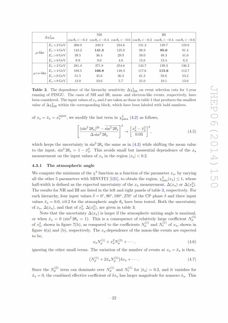
The dependences on Ecutν and cos θcutz are shown in table 2 where the input values of

δ and xa are chosen corresponding to the smallest value of ∆χ2MH in each block of table 1

respectively. We observe that the results depend strongly on the range of Eν and cos θz.

For instance, when Ecutν is raised from 6GeV to 8GeV, ∆χ2

MH drops by nearly a factor of

3 ∼ 7, while for Eν > 8GeV, changing of the zenith angle coverage from cos θz < −0.4 to

cos θz < −0.6 reduces ∆χ2MH by further factor of 2. It is therefore very important to have

low energy threshold of the detector and to study the smearing effects in detail.

4.3 The atmospheric angle and its octant

Once the mass hierarchy is determined, χ2 fit can be performed with the correct mass

hierarchy as an input, and the same χ2 function (4.1) can be used to measure the atmo-

spheric mixing angle and its octant discussed here, as well as the CP phase δ which will

be discussed in section 4.4. In order to make the global minimum to be at the input value

– 21 –

JHEP06(2014)150

∆χ2

MH

NH IH

cos θz<−0.2 cos θz<−0.4 cos θz<−0.6 cos θz<−0.2 cos θz<−0.4 cos θz<−0.6

µ-like

Eν >2GeV 260.0 249.2 234.6 131.2 129.7 123.6

Eν >4GeV 143.2 141.5 125.0 98.9 95.6 91.4

Eν >6GeV 39.5 36.4 29.9 50.0 48.3 41.0

Eν >8GeV 9.9 9.0 4.8 15.6 13.4 6.3

µ+e-like

Eν >2GeV 281.4 271.8 254.6 142.7 139.3 136.2

Eν >4GeV 169.5 166.8 148.3 117.6 115.6 112.7

Eν >6GeV 51.5 45.6 36.3 61.2 58.6 53.2

Eν >8GeV 12.0 10.6 5.7 21.0 19.1 13.6

Table 2. The dependence of the hierarchy sensitivity ∆χ2MH on event selection cuts for 1-year

running of PINGU. The cases of NH and IH, muon- and electron-like events, respectively, have

been considered. The input values of xa and δ are taken as those in table 1 that produces the smallest

value of ∆χ2MH within the corresponding block, which have been labeled with bold numbers.

of xa = xa = xinputa , we modify the last term in χ2para (4.2) as follows,

[(sin2 2θa)

fit − sin2 2θa

∆sin2 2θa

]2→[x2a − x2a0.03

]2, (4.5)

which keeps the uncertainty in sin2 2θa the same as in (4.3) while shifting the mean value

to the input, sin2 2θa = 1 − x2a. This avoids small but inessential dependence of the xameasurement on the input values of xa in the region |xa| < 0.2.

4.3.1 The atmospheric angle

We compute the minimum of the χ2 function as a function of the parameter xa, by varying

all the other 5 parameters with MINUIT2 [121], to obtain the region, χ2min(xa) ≤ 1, whose

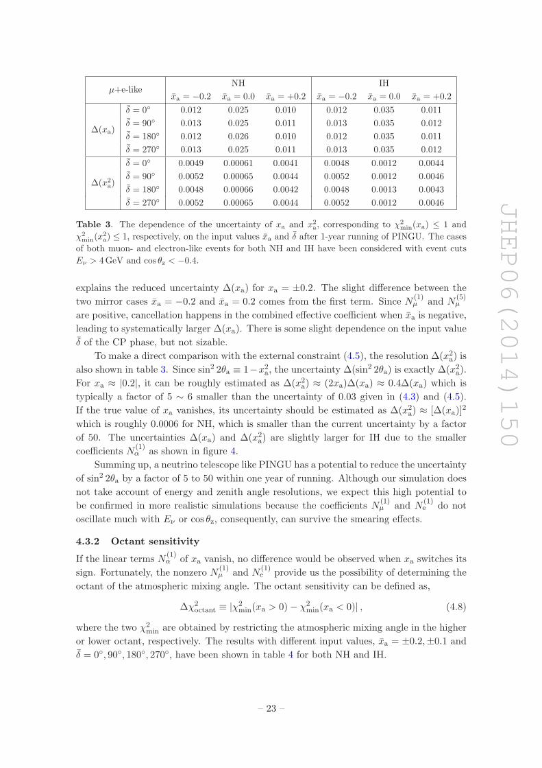
half-width is defined as the expected uncertainty of the xa measurement, ∆(xa) or ∆(x2a).

The results for NH and IH are listed in the left and right panels of table 3, respectively. For

each hierarchy, four input values δ = 0◦, 90◦, 180◦, 270◦ of the CP phase δ and three input

values xa = 0.0,±0.2 for the atmospheric angle θa have been tested. Both the uncertainty

of xa, ∆(xa), and that of x2a, ∆(x2a), are given in table 3.

Note that the uncertainty ∆(xa) is larger if the atmospheric mixing angle is maximal,

or when xa = 0 (sin2 2θa = 1). This is a consequence of relatively large coefficient N(5)µ

of x2a, shown in figure 7(b), as compared to the coefficients N(1)µ and N

(1)e of xa, shown in

figure 4(a) and (b), respectively. The xa-dependence of the muon-like events are expected

to be,

xaN(1)µ + x2aN

(5)µ + · · · , (4.6)

ignoring the other small terms. The variation of the number of events at xa = xa is then,

(N (1)

µ + 2xaN(5)µ

)δxa + · · · . (4.7)

Since the N(5)µ term can dominate over N

(1)µ and N

(1)e for |xa| = 0.2, and it vanishes for

xa = 0, the combined effective coefficient of δxa has larger magnitude for nonzero xa. This

– 22 –

JHEP06(2014)150

µ+e-likeNH IH

xa = −0.2 xa = 0.0 xa = +0.2 xa = −0.2 xa = 0.0 xa = +0.2

∆(xa)

δ = 0◦ 0.012 0.025 0.010 0.012 0.035 0.011

δ = 90◦ 0.013 0.025 0.011 0.013 0.035 0.012

δ = 180◦ 0.012 0.026 0.010 0.012 0.035 0.011

δ = 270◦ 0.013 0.025 0.011 0.013 0.035 0.012

∆(x2a)

δ = 0◦ 0.0049 0.00061 0.0041 0.0048 0.0012 0.0044

δ = 90◦ 0.0052 0.00065 0.0044 0.0052 0.0012 0.0046

δ = 180◦ 0.0048 0.00066 0.0042 0.0048 0.0013 0.0043

δ = 270◦ 0.0052 0.00065 0.0044 0.0052 0.0012 0.0046

Table 3. The dependence of the uncertainty of xa and x2a, corresponding to χ2

min(xa) ≤ 1 and

χ2min(x

2a) ≤ 1, respectively, on the input values xa and δ after 1-year running of PINGU. The cases

of both muon- and electron-like events for both NH and IH have been considered with event cuts

Eν > 4GeV and cos θz < −0.4.

explains the reduced uncertainty ∆(xa) for xa = ±0.2. The slight difference between the

two mirror cases xa = −0.2 and xa = 0.2 comes from the first term. Since N(1)µ and N

(5)µ

are positive, cancellation happens in the combined effective coefficient when xa is negative,

leading to systematically larger ∆(xa). There is some slight dependence on the input value

δ of the CP phase, but not sizable.

To make a direct comparison with the external constraint (4.5), the resolution ∆(x2a) is

also shown in table 3. Since sin2 2θa ≡ 1−x2a, the uncertainty ∆(sin2 2θa) is exactly ∆(x2a).

For xa ≈ |0.2|, it can be roughly estimated as ∆(x2a) ≈ (2xa)∆(xa) ≈ 0.4∆(xa) which is

typically a factor of 5 ∼ 6 smaller than the uncertainty of 0.03 given in (4.3) and (4.5).

If the true value of xa vanishes, its uncertainty should be estimated as ∆(x2a) ≈ [∆(xa)]2

which is roughly 0.0006 for NH, which is smaller than the current uncertainty by a factor

of 50. The uncertainties ∆(xa) and ∆(x2a) are slightly larger for IH due to the smaller

coefficients N(1)α as shown in figure 4.

Summing up, a neutrino telescope like PINGU has a potential to reduce the uncertainty

of sin2 2θa by a factor of 5 to 50 within one year of running. Although our simulation does

not take account of energy and zenith angle resolutions, we expect this high potential to

be confirmed in more realistic simulations because the coefficients N(1)µ and N

(1)e do not

oscillate much with Eν or cos θz, consequently, can survive the smearing effects.

4.3.2 Octant sensitivity

If the linear terms N(1)α of xa vanish, no difference would be observed when xa switches its

sign. Fortunately, the nonzero N(1)µ and N

(1)e provide us the possibility of determining the

octant of the atmospheric mixing angle. The octant sensitivity can be defined as,

∆χ2octant ≡ |χ2

min(xa > 0)− χ2min(xa < 0)| , (4.8)

where the two χ2min are obtained by restricting the atmospheric mixing angle in the higher

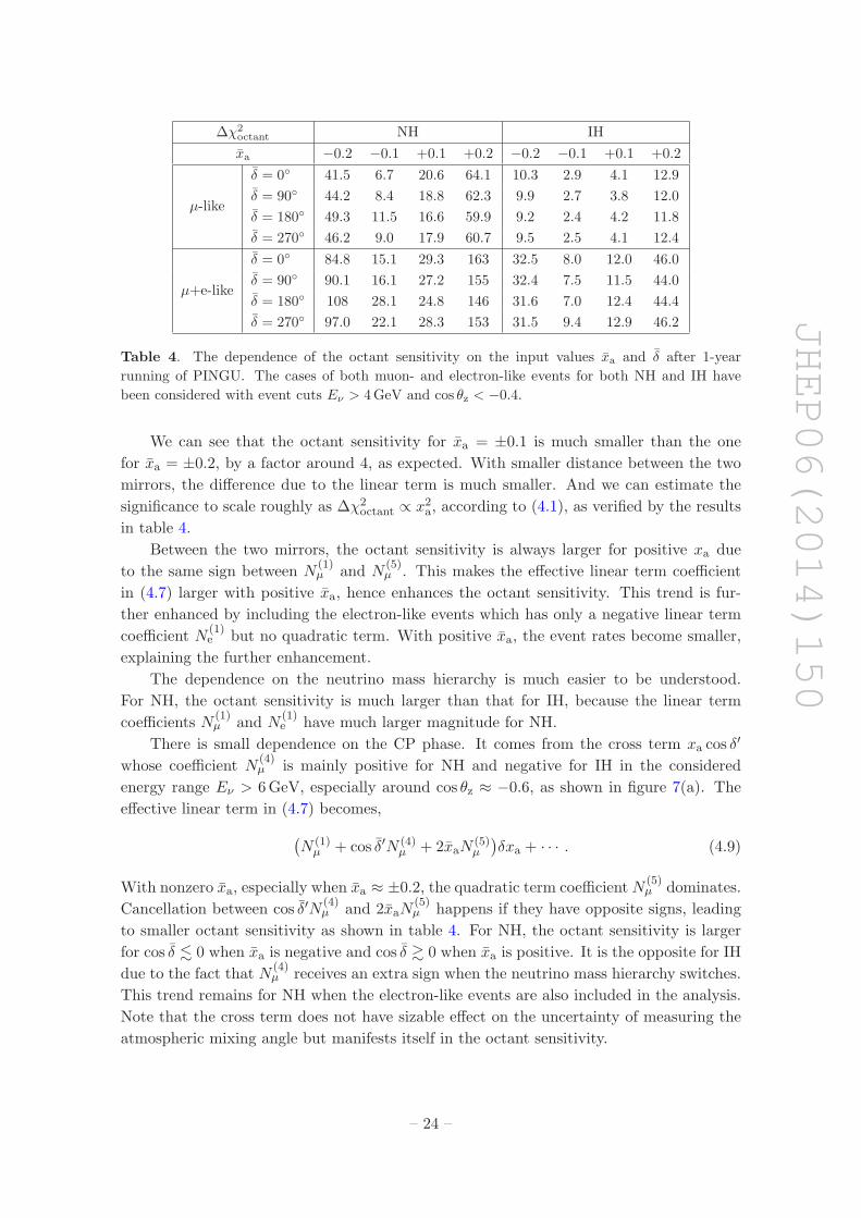
or lower octant, respectively. The results with different input values, xa = ±0.2,±0.1 and

δ = 0◦, 90◦, 180◦, 270◦, have been shown in table 4 for both NH and IH.

– 23 –

JHEP06(2014)150

∆χ2octant NH IH

xa −0.2 −0.1 +0.1 +0.2 −0.2 −0.1 +0.1 +0.2

µ-like

δ = 0◦ 41.5 6.7 20.6 64.1 10.3 2.9 4.1 12.9

δ = 90◦ 44.2 8.4 18.8 62.3 9.9 2.7 3.8 12.0

δ = 180◦ 49.3 11.5 16.6 59.9 9.2 2.4 4.2 11.8

δ = 270◦ 46.2 9.0 17.9 60.7 9.5 2.5 4.1 12.4

µ+e-like

δ = 0◦ 84.8 15.1 29.3 163 32.5 8.0 12.0 46.0

δ = 90◦ 90.1 16.1 27.2 155 32.4 7.5 11.5 44.0

δ = 180◦ 108 28.1 24.8 146 31.6 7.0 12.4 44.4

δ = 270◦ 97.0 22.1 28.3 153 31.5 9.4 12.9 46.2

Table 4. The dependence of the octant sensitivity on the input values xa and δ after 1-year

running of PINGU. The cases of both muon- and electron-like events for both NH and IH have

been considered with event cuts Eν > 4GeV and cos θz < −0.4.

We can see that the octant sensitivity for xa = ±0.1 is much smaller than the one

for xa = ±0.2, by a factor around 4, as expected. With smaller distance between the two

mirrors, the difference due to the linear term is much smaller. And we can estimate the

significance to scale roughly as ∆χ2octant ∝ x2a, according to (4.1), as verified by the results

in table 4.

Between the two mirrors, the octant sensitivity is always larger for positive xa due

to the same sign between N(1)µ and N

(5)µ . This makes the effective linear term coefficient

in (4.7) larger with positive xa, hence enhances the octant sensitivity. This trend is fur-

ther enhanced by including the electron-like events which has only a negative linear term

coefficient N(1)e but no quadratic term. With positive xa, the event rates become smaller,

explaining the further enhancement.

The dependence on the neutrino mass hierarchy is much easier to be understood.

For NH, the octant sensitivity is much larger than that for IH, because the linear term

coefficients N(1)µ and N

(1)e have much larger magnitude for NH.

There is small dependence on the CP phase. It comes from the cross term xa cos δ′

whose coefficient N(4)µ is mainly positive for NH and negative for IH in the considered

energy range Eν > 6GeV, especially around cos θz ≈ −0.6, as shown in figure 7(a). The

effective linear term in (4.7) becomes,

(N (1)

µ + cos δ′N (4)µ + 2xaN

(5)µ

)δxa + · · · . (4.9)

With nonzero xa, especially when xa ≈ ±0.2, the quadratic term coefficientN(5)µ dominates.

Cancellation between cos δ′N(4)µ and 2xaN

(5)µ happens if they have opposite signs, leading

to smaller octant sensitivity as shown in table 4. For NH, the octant sensitivity is larger

for cos δ . 0 when xa is negative and cos δ & 0 when xa is positive. It is the opposite for IH

due to the fact that N(4)µ receives an extra sign when the neutrino mass hierarchy switches.

This trend remains for NH when the electron-like events are also included in the analysis.

Note that the cross term does not have sizable effect on the uncertainty of measuring the

atmospheric mixing angle but manifests itself in the octant sensitivity.

– 24 –

JHEP06(2014)150

∆(δ)NH IH

xa = −0.2 xa = 0.0 xa = +0.2 xa = −0.2 xa = 0.0 xa = +0.2

Eν > 6GeV

δ = 0◦ 23◦ 23◦ 22◦ 49◦ 48◦ 48◦

δ = 90◦ 20◦ 20◦ 18◦ 41◦ 41◦ 38◦

δ = 180◦ 23◦ 23◦ 21◦ 49◦ 48◦ 48◦

δ = 270◦ 20◦ 20◦ 18◦ 41◦ 41◦ 38◦

Eν > 4GeV

δ = 0◦ 15◦ 14◦ 14◦ 32◦ 31◦ 32◦

δ = 90◦ 13◦ 12◦ 11◦ 29◦ 29◦ 28◦

δ = 180◦ 15◦ 14◦ 14◦ 32◦ 31◦ 32◦

δ = 270◦ 13◦ 12◦ 11◦ 29◦ 29◦ 28◦

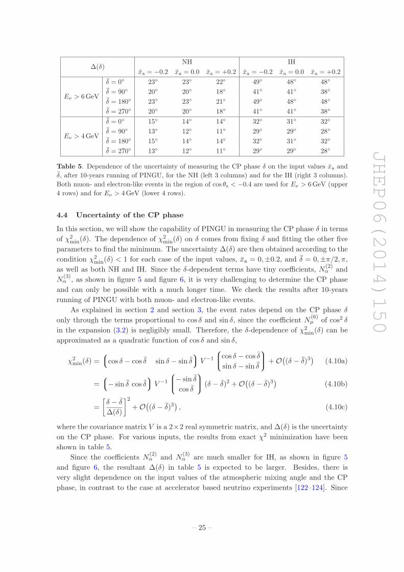
Table 5. Dependence of the uncertainty of measuring the CP phase δ on the input values xa and

δ, after 10-years running of PINGU, for the NH (left 3 columns) and for the IH (right 3 columns).

Both muon- and electron-like events in the region of cos θz < −0.4 are used for Eν > 6GeV (upper

4 rows) and for Eν > 4GeV (lower 4 rows).

4.4 Uncertainty of the CP phase

In this section, we will show the capability of PINGU in measuring the CP phase δ in terms

of χ2min(δ). The dependence of χ2

min(δ) on δ comes from fixing δ and fitting the other five

parameters to find the minimum. The uncertainty ∆(δ) are then obtained according to the

condition χ2min(δ) < 1 for each case of the input values, xa = 0,±0.2, and δ = 0,±π/2, π,

as well as both NH and IH. Since the δ-dependent terms have tiny coefficients, N(2)α and

N(3)α , as shown in figure 5 and figure 6, it is very challenging to determine the CP phase

and can only be possible with a much longer time. We check the results after 10-years

running of PINGU with both muon- and electron-like events.

As explained in section 2 and section 3, the event rates depend on the CP phase δ

only through the terms proportional to cos δ and sin δ, since the coefficient N(6)µ of cos2 δ

in the expansion (3.2) is negligibly small. Therefore, the δ-dependence of χ2min(δ) can be

approximated as a quadratic function of cos δ and sin δ,

χ2min(δ) =

cos δ − cos δ sin δ − sin δ

V −1

cos δ − cos δ

sin δ − sin δ

+O

((δ − δ)3

)(4.10a)

=− sin δ cos δ

V −1

− sin δ

cos δ

(δ − δ)2 +O

((δ − δ)3

)(4.10b)

=

[δ − δ

∆(δ)

]2+O

((δ − δ)3

), (4.10c)

where the covariance matrix V is a 2×2 real symmetric matrix, and ∆(δ) is the uncertainty

on the CP phase. For various inputs, the results from exact χ2 minimization have been

shown in table 5.

Since the coefficients N(2)α and N

(3)α are much smaller for IH, as shown in figure 5

and figure 6, the resultant ∆(δ) in table 5 is expected to be larger. Besides, there is

very slight dependence on the input values of the atmospheric mixing angle and the CP

phase, in contrast to the case at accelerator based neutrino experiments [122–124]. Since

– 25 –

JHEP06(2014)150

the δ-dependence of the event rates occurs only through terms of cos δ and sin δ, the

χ2min(δ) function is a periodic function of δ. It vanishes at δ = δ and has only one period of

oscillation in the range of [0, 2π] with peak around |δ−δ| ≈ π. With energy cut Eν > 6GeV,

the maximum value of χ2min(δ) is around 25 ∼ 40 for NH, and just 6 ∼ 8 for IH, depending

on the input values of xa and δ. The value increases to around 12 ∼ 16 for IH if we include

events down to Eν = 4GeV. The function χ2min(δ) can be approximated by a quadratic

function (4.10) of δ − δ up to more than 3σ for all the results quoted in table 5 with the

only exception of Eν > 6GeV for IH where it holds up only to around 2.5σ.

There is some slight xa-dependence of the uncertainty ∆(δ), which can then be read

off directly by expressing the covariance matrix in terms of the decomposition coefficients,

N(2)α + xaN

(4)α and N

(3)α , for an input value of xa = xa as follows,

V −1 = V −1µ + V −1

e , (4.11a)

V −1α =

∫dEνd cos θz

N(0)α +N

(1)α xa+N

(5)α x2a

(1− x2a)

[N

(2)α +N

(4)α xa

]2N

(3)α

[N

(2)α +N

(4)α xa

]

N(3)α

[N

(2)α +N

(4)α xa

] [N

(3)α

]2

,

(4.11b)

where we neglect the small δ-dependent terms in the denominator of (4.11b). SinceN(2)µ and

N(4)µ share the same sign in the considered energy range of Eν > 6GeV, especially around

cos θz ≈ −0.8 ∼ −0.6, as shown in figure 5, figure 6, and figure 7, the combination N(2)µ +

N(4)µ xa has larger magnitude when xa is positive. This explains the reduced uncertainty

at xa = +0.2. Note that there is an overall factor 1 − x2a due to the modulation cos δ′ =√1− x2a cos δ and sin δ′ =

√1− x2a sin δ. It can increase the CP phase uncertainty ∆(δ) if

the atmospheric mixing angle is not maximal, namely 1− x2a < 1.

The δ dependence of ∆(δ) can be expressed as,

∆(δ) =[(V −1)11 sin

2 δ − 2(V −1)12 sin δ cos δ + (V −1)22 cos2 δ]−1/2

. (4.12)

If the elements (V −1)11, (V −1)12, and (V −1)22 have same size, the uncertainty on the

CP phase, ∆(δ), becomes δ-independent. Otherwise, ∆(δ) would receive some varia-

tion. We can treat cos δ and sin δ as independent functions with nominal uncertainties

∆(cos δ) =√V11, ∆(sin δ) =

√V22, and V12 =

√V11

√V22ρ. The above approximation for

the covariance matrices gives, for xa = 0,

∆(cos δ) = 0.65 , ∆(sin δ) = 0.97 , ρ = −0.29 for NH (µ-like) , (4.13a)

∆(cos δ) = 0.38 , ∆(sin δ) = 0.40 , ρ = −0.21 for NH (e-like) , (4.13b)

∆(cos δ) = 0.33 , ∆(sin δ) = 0.37 , ρ = −0.23 for NH (µ+e-like) , (4.13c)

and,

∆(cos δ) = 1.43 , ∆(sin δ) = 1.79 , ρ = −0.27 for IH (µ-like) , (4.14a)

∆(cos δ) = 0.78 , ∆(sin δ) = 0.87 , ρ = −0.23 for IH (e-like) , (4.14b)

∆(cos δ) = 0.69 , ∆(sin δ) = 0.78 , ρ = −0.24 for IH (µ+e-like) , (4.14c)

– 26 –

JHEP06(2014)150

for the integration region of 6GeV < Eν < 20GeV and cos θz < −0.4 with 10 years running

of PINGU.

From the results of (4.13) and (4.14), we find that the uncertainties ∆(sin δ) and

∆(cos δ) are rather large when only the muon-like events of Eν > 6GeV are used in the

analysis. This is especially the case of IH, for which the uncertainties are larger than unity

even after 10-years of running. In other words, the uncertainty ∆(δ) can be rather broad.

Therefore, the electron-like events are essential to measure the CP phase.

Generally speaking, ∆(cos δ) is slightly smaller than ∆(sin δ) due to larger magnitude of

N(2)α , resulting in slightly smaller uncertainties ∆(δ) at δ = ±90◦ than those at δ = 0◦, 180◦.

In addition, the correlation turns out to be small |ρ| ∼ 0.2 and negative for all the cases.

From the combined results in (4.13) and (4.14), we can estimate the smallest and the largest

uncertainty of ∆(δ) as a function of δ,

∆(δ)max = 23◦ @ δ = 32◦, 212◦ for NH (µ+e-like) , (4.15a)

∆(δ)min = 17◦ @ δ = 122◦, 302◦ for NH (µ+e-like) , (4.15b)

for NH, and

∆(δ)max = 48◦ @ δ = 32◦, 212◦ for IH (µ+e-like) , (4.16a)

∆(δ)min = 36◦ @ δ = 122◦, 302◦ for IH (µ+e-like) , (4.16b)

for IH. All the results quoted in table 5 lie within the above range. The largest differences

are found to be about a few degrees for the IH case with Eν > 6GeV.

5 Conclusions and outlook

In this work, we develop a general decomposition formalism in the propagation basis, which

is extremely useful for the phenomenological study of neutrino oscillation. It can analyt-

ically separate the contributions of the three unknown parameters, namely, the neutrino

mass hierarchy, the atmospheric mixing angle, and the CP phase. In this way, the pattern

behind χ2 minimization can be revealed clearly, especially for atmospheric neutrino which

experiences very complicated Earth matter profile. Hence, it can serve as a complementary

tool to the neutrino oscillogram. The latter is designed for the overall pattern, especially

the resonance behaviors, in the atmospheric neutrino oscillations, while our decomposi-

tion method can unveil more hidden structures behind the oscillogram. In addition, the

decomposition method can apply generally to any type of neutrino oscillation experiment.

To illustrate the powerfulness of this decomposition formalism, we study in detail the

ability of PINGU in determining the neutrino mass hierarchy, the atmospheric angle θa and

its octant, as well as the CP phase δ by measuring the oscillation pattern of atmospheric

neutrinos. Both muon- and electron-like events have been considered. Our results suggest

that PINGU has the potential to determine the mass hierarchy and the octant of the

atmospheric mixing angle θa within one year of operation if the neutrino energy and the

zenith angle can be measured accurately in the region Eν = 4 ∼ 20GeV and cos θz < −0.4.

The uncertainty of measuring the value of θa can be reduced by a factor of 5 ∼ 30, while

– 27 –

JHEP06(2014)150

the determination of the CP phase δ is significantly more challenging. The dependence

on the input values of the neutrino mass hierarchy, the atmospheric mixing angle, and the

CP phase can be understood in our decomposition formalism. Our findings merit a serious

investigation of the physics potential of PINGU with realistic detector response which we

expect to be underway within the IceCube/PINGU Collaboration.

Acknowledgments

We thank Naotoshi Okamura for stimulating discussions in the early stage of our investiga-

tion. SFG is grateful to Hong-Jian He for kind support and Center for High Energy Physics

of Tsinghua University (TUHEP), where part of this work is done, for hospitality. JSPS

has provided SFG a generous postdoc fellowship, which is deeply appreciated, to continue

the study at KEK. This work is supported in part by Grant-in-Aid for Scientific research

(No. 25400287) from JSPS. CR is grateful for support from the Center for Cosmology and

AstroParticle Physics (CCAPP) at The Ohio State University, where part of this work was

performed. This work is supported in part by the Basic Science Research Program through

the National Research Foundation of Korea funded by the Ministry of Education, Science

and Technology (NRF-2013R1A1A1007068).

A Atmospheric neutrino oscillation

In this appendix, we introduce the input and method that we used to evaluate the atmo-

spheric neutrino oscillation in this study. They include the atmospheric neutrino fluxes,

interaction cross sections, and an energy-dependent effective detector volume, the Earth

matter density profile and the numerical procedure.

A.1 Atmospheric neutrino flux, cross sections and effective volume

The atmospheric neutrino flux depends on many factors. First, it varies with the geo-

graphic location, mainly due to the earth magnetic field at the source regions. In addition,

it dependents on the neutrino momentum direction, the zenith and the azimuth angles.

Seasonal effects can also modulate the neutrino flux. For our study, we use an annual

and azimuth angle averaged neutrino flux computed for the South Pole [102]. The earth

magnetic field effect, which introduces the largest modification on neutrino fluxes, depend-

ing on the position, are mostly relevant for neutrino energies below the one considered in

this study; therefore our results can be easily transferred to detectors at other geographic

locations. With these factors taken into consideration, the neutrino flux is a function of

neutrino energy and the zenith angle.

The energy dependence of the atmospheric neutrino flux is shown in figure 8(a). It

can be seen that νµ and νµ fluxes dominate over the νe and νe fluxes. They drop very

quickly with increasing energy, decreasing by four orders of magnitude from Eν = 1GeV

to Eν = 20GeV. For both flavors, the antineutrino flux is slightly smaller than the neutrino

flux due to an asymmetry between the π+ and π− production spectra in cosmic ray air-

showers [102].

– 28 –

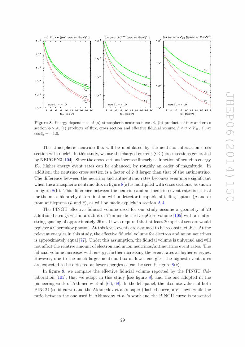
JHEP06(2014)150

10-3

10-2

10-1

100

101

102

2 4 6 8 10 12 14 16 18 20Eν [GeV]

(a) Flux φ [(m2 sec sr GeV)-1]

cosθz = -1.0

νµ

—νµ

νe

—νe

10-4

10-3

10-2

10-1

2 4 6 8 10 12 14 16 18 20Eν [GeV]

(b) φ×σ [10-38 (sec sr GeV)-1]

cosθz = -1.0

νµ

—νµ

νe

—νe

101

102

103

104

2 4 6 8 10 12 14 16 18 20Eν [GeV]

(c) φ×σ×ρ×Veff [(year sr GeV)-1]

cosθz = -1.0

νµ

—νµ

νe

—νe

Figure 8. Energy dependence of (a) atmospheric neutrino fluxes φ, (b) products of flux and cross

section φ × σ, (c) products of flux, cross section and effective fiducial volume φ × σ × Veff , all at

cos θz = −1.0.

The atmospheric neutrino flux will be modulated by the neutrino interaction cross

section with nuclei. In this study, we use the charged current (CC) cross sections generated

by NEUGEN3 [104]. Since the cross sections increase linearly as function of neutrino energy

Eν , higher energy event rates can be enhanced, by roughly an order of magnitude. In

addition, the neutrino cross section is a factor of 2–3 larger than that of the antineutrino.

The difference between the neutrino and antineutrino rates becomes even more significant

when the atmospheric neutrino flux in figure 8(a) is multiplied with cross sections, as shown

in figure 8(b). This difference between the neutrino and antineutrino event rates is critical

for the mass hierarchy determination with a detector incapable of telling leptons (µ and e)

from antileptons (µ and e), as will be made explicit in section A.4.

The PINGU effective fiducial volume used for our study assume a geometry of 20

additional strings within a radius of 75m inside the DeepCore volume [105] with an inter-

string spacing of approximately 26m. It was required that at least 20 optical sensors would

register a Cherenkov photon. At this level, events are assumed to be reconstructable. At the

relevant energies in this study, the effective fiducial volume for electron and muon neutrinos

is approximately equal [77]. Under this assumption, the fiducial volume is universal and will

not affect the relative amount of electron and muon neutrinos/antineutrino event rates. The

fiducial volume increases with energy, further increasing the event rates at higher energies.

However, due to the much larger neutrino flux at lower energies, the highest event rates

are expected to be detected at lower energies as can be seen in figure 8(c).

In figure 9, we compare the effective fiducial volume reported by the PINGU Col-

laboration [105], that we adopt in this study [see figure 8], and the one adopted in the

pioneering work of Akhmedov et al. [66, 68]. In the left panel, the absolute values of both

PINGU (solid curve) and the Akhmedov et al.’s paper (dashed curve) are shown while the

ratio between the one used in Akhmedov et al.’s work and the PINGU curve is presented

– 29 –

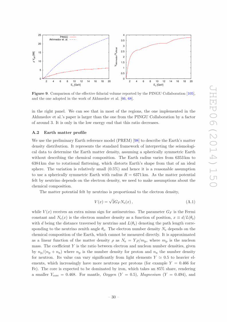
JHEP06(2014)150

0

5

10

15

20

25

2 4 6 8 10 12 14 16 18 20

ρ V

eff [

Mt]

Eν [GeV]

PINGUAkhmedov et. al.

0

0.5

1

1.5

2

2.5

3

3.5

4

2 4 6 8 10 12 14 16 18 20

VA

khm

edov/V

offic

ial

Eν [GeV]

Figure 9. Comparison of the effective fiducial volume reported by the PINGU Collaboration [105],

and the one adopted in the work of Akhmedov et al. [66, 68].

in the right panel. We can see that in most of the regions, the one implemented in the

Akhmedov et al.’s paper is larger than the one from the PINGU Collaboration by a factor

of around 3. It is only in the low energy end that this ratio decreases.

A.2 Earth matter profile

We use the preliminary Earth reference model (PREM) [98] to describe the Earth’s matter

density distribution. It represents the standard framework of interpreting the seismologi-

cal data to determine the Earth matter density, assuming a spherically symmetric Earth

without describing the chemical composition. The Earth radius varies from 6353 km to

6384 km due to rotational flattening, which distorts Earth’s shape from that of an ideal

sphere. The variation is relatively small (0.5%) and hence it is a reasonable assumption

to use a spherically symmetric Earth with radius R = 6371 km. As the matter potential

felt by neutrino depends on the electron density, we need to make assumptions about the

chemical composition.

The matter potential felt by neutrino is proportional to the electron density,

V (x) =√2GFNe(x) , (A.1)

while V (x) receives an extra minus sign for antineutrino. The parameter GF is the Fermi

constant and Ne(x) is the electron number density as a function of position, x ≡ d/L(θz)

with d being the distance traversed by neutrino and L(θz) denoting the path length corre-

sponding to the neutrino zenith angle θz. The electron number density Ne depends on the

chemical composition of the Earth, which cannot be measured directly. It is approximated

as a linear function of the matter density ρ as Ne = Y ρ/mp, where mp is the nucleon

mass. The coefficient Y is the ratio between electron and nucleon number densities, given

by np/(np + nn) where np is the number density for proton and nn the number density

for neutron. Its value can vary significantly from light elements Y ≃ 0.5 to heavier el-

ements, which increasingly have more neutrons per protons (for example Y = 0.466 for

Fe). The core is expected to be dominated by iron, which takes an 85% share, rendering

a smaller Ycore = 0.468. For mantle, Oxygen (Y = 0.5), Magnesium (Y = 0.494), and

– 30 –

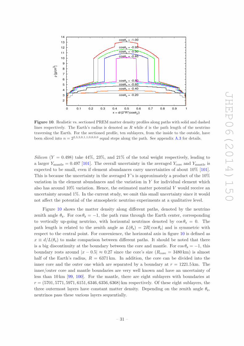
JHEP06(2014)150

2

3

4

5

6

7

8

9

10

11

12

13

14

0 0.1 0.2 0.3 0.4 0.5 0.6 0.7 0.8 0.9 1

ρ [g

/cm

3 ]

x = d/(2*R*|cosθz|)

cosθz = -1.00

cosθz = -0.95

cosθz = -0.90

cosθz = -0.85

cosθz = -0.80

cosθz = -0.60

cosθz = -0.40

cosθz = -0.20

Figure 10. Realistic vs. sectioned PREM matter density profiles along paths with solid and dashed

lines respectively. The Earth’s radius is denoted as R while d is the path length of the neutrino

traversing the Earth. For the sectioned profile, ten sublayers, from the inside to the outside, have

been sliced into n = 22,3,3,0,1,1,0,0,0,0 equal steps along the path. See appendix A.3 for details.

Silicon (Y = 0.498) take 44%, 23%, and 21% of the total weight respectively, leading to

a larger Ymantle = 0.497 [101]. The overall uncertainty in the averaged Ycore and Ymantle is

expected to be small, even if element abundances carry uncertainties of about 10% [101].

This is because the uncertainty in the averaged Y ’s is approximately a product of the 10%

variation in the element abundances and the variation in Y for individual element which

also has around 10% variation. Hence, the estimated matter potential V would receive an

uncertainty around 1%. In the current study, we omit this small uncertainty since it would

not affect the potential of the atmospheric neutrino experiments at a qualitative level.

Figure 10 shows the matter density along different paths, denoted by the neutrino

zenith angle θz. For cos θz = −1, the path runs through the Earth center, corresponding

to vertically up-going neutrino, with horizontal neutrinos denoted by cos θz = 0. The

path length is related to the zenith angle as L(θz) = 2R| cos θz| and is symmetric with

respect to the central point. For convenience, the horizontal axis in figure 10 is defined as

x ≡ d/L(θz) to make comparison between different paths. It should be noted that there

is a big discontinuity at the boundary between the core and mantle. For cos θz = −1, this

boundary rests around |x − 0.5| ≈ 0.27 since the core’s size (Rcore = 3480 km) is almost

half of the Earth’s radius, R = 6371 km. In addition, the core can be divided into the

inner core and the outer one which are separated by a boundary at r = 1221.5 km. The

inner/outer core and mantle boundaries are very well known and have an uncertainty of

less than 10 km [99, 100]. For the mantle, there are eight sublayers with boundaries at

r = (5701, 5771, 5971, 6151, 6346, 6356, 6368) km respectively. Of these eight sublayers, the

three outermost layers have constant matter density. Depending on the zenith angle θz,

neutrinos pass these various layers sequentially.

– 31 –

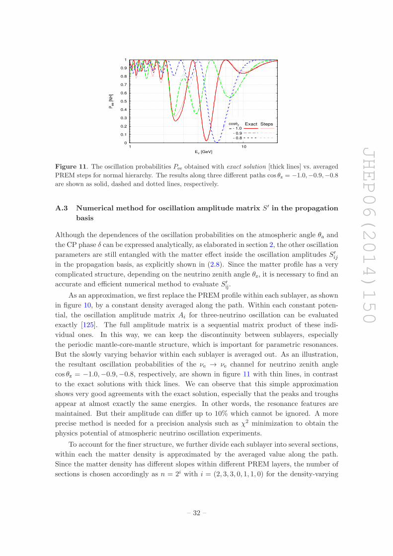
JHEP06(2014)150

0

0.1

0.2

0.3

0.4

0.5

0.6

0.7

0.8

0.9

1

1 10

Pee

[NH

]

Eν [GeV]

Exact Stepscosθz

= - 1.0

- 0.9

- 0.8

Figure 11. The oscillation probabilities Pee obtained with exact solution [thick lines] vs. averaged

PREM steps for normal hierarchy. The results along three different paths cos θz = −1.0,−0.9,−0.8

are shown as solid, dashed and dotted lines, respectively.

A.3 Numerical method for oscillation amplitude matrix S′ in the propagation

basis

Although the dependences of the oscillation probabilities on the atmospheric angle θa and

the CP phase δ can be expressed analytically, as elaborated in section 2, the other oscillation

parameters are still entangled with the matter effect inside the oscillation amplitudes S′ij

in the propagation basis, as explicitly shown in (2.8). Since the matter profile has a very

complicated structure, depending on the neutrino zenith angle θz, it is necessary to find an

accurate and efficient numerical method to evaluate S′ij.

As an approximation, we first replace the PREM profile within each sublayer, as shown

in figure 10, by a constant density averaged along the path. Within each constant poten-

tial, the oscillation amplitude matrix Ai for three-neutrino oscillation can be evaluated

exactly [125]. The full amplitude matrix is a sequential matrix product of these indi-

vidual ones. In this way, we can keep the discontinuity between sublayers, especially

the periodic mantle-core-mantle structure, which is important for parametric resonances.

But the slowly varying behavior within each sublayer is averaged out. As an illustration,

the resultant oscillation probabilities of the νe → νe channel for neutrino zenith angle

cos θz = −1.0,−0.9,−0.8, respectively, are shown in figure 11 with thin lines, in contrast

to the exact solutions with thick lines. We can observe that this simple approximation

shows very good agreements with the exact solution, especially that the peaks and troughs

appear at almost exactly the same energies. In other words, the resonance features are

maintained. But their amplitude can differ up to 10% which cannot be ignored. A more

precise method is needed for a precision analysis such as χ2 minimization to obtain the

physics potential of atmospheric neutrino oscillation experiments.

To account for the finer structure, we further divide each sublayer into several sections,

within each the matter density is approximated by the averaged value along the path.

Since the matter density has different slopes within different PREM layers, the number of

sections is chosen accordingly as n = 2i with i = (2, 3, 3, 0, 1, 1, 0) for the density-varying

– 32 –

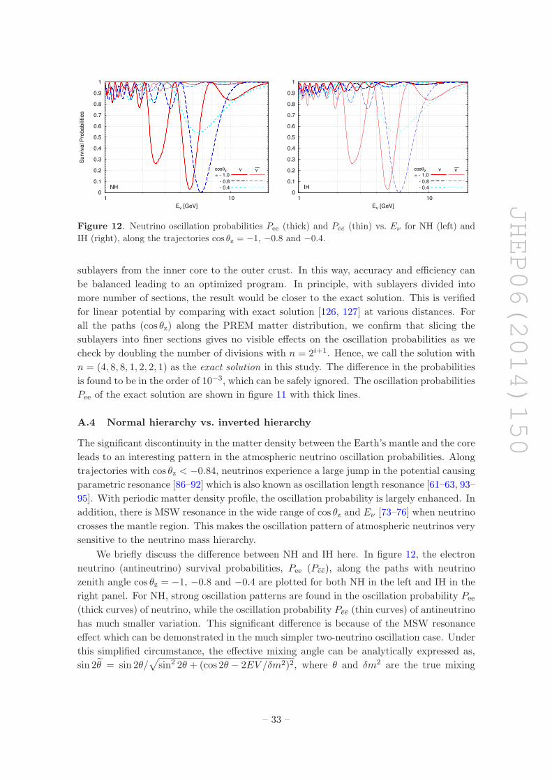
JHEP06(2014)150

0

0.1

0.2

0.3

0.4

0.5

0.6

0.7

0.8

0.9

1

1 10

Surv

ival P

robabili

ties

Eν [GeV]

NH

ν —νcosθz

= - 1.0

- 0.8

- 0.4 0

0.1

0.2

0.3

0.4

0.5

0.6

0.7

0.8

0.9

1

1 10

Eν [GeV]

IH

ν —νcosθz

= - 1.0

- 0.8

- 0.4

Figure 12. Neutrino oscillation probabilities Pee (thick) and Pee (thin) vs. Eν for NH (left) and

IH (right), along the trajectories cos θz = −1, −0.8 and −0.4.

sublayers from the inner core to the outer crust. In this way, accuracy and efficiency can

be balanced leading to an optimized program. In principle, with sublayers divided into

more number of sections, the result would be closer to the exact solution. This is verified

for linear potential by comparing with exact solution [126, 127] at various distances. For

all the paths (cos θz) along the PREM matter distribution, we confirm that slicing the

sublayers into finer sections gives no visible effects on the oscillation probabilities as we

check by doubling the number of divisions with n = 2i+1. Hence, we call the solution with

n = (4, 8, 8, 1, 2, 2, 1) as the exact solution in this study. The difference in the probabilities

is found to be in the order of 10−3, which can be safely ignored. The oscillation probabilities

Pee of the exact solution are shown in figure 11 with thick lines.

A.4 Normal hierarchy vs. inverted hierarchy

The significant discontinuity in the matter density between the Earth’s mantle and the core

leads to an interesting pattern in the atmospheric neutrino oscillation probabilities. Along

trajectories with cos θz < −0.84, neutrinos experience a large jump in the potential causing

parametric resonance [86–92] which is also known as oscillation length resonance [61–63, 93–

95]. With periodic matter density profile, the oscillation probability is largely enhanced. In

addition, there is MSW resonance in the wide range of cos θz and Eν [73–76] when neutrino

crosses the mantle region. This makes the oscillation pattern of atmospheric neutrinos very

sensitive to the neutrino mass hierarchy.

We briefly discuss the difference between NH and IH here. In figure 12, the electron

neutrino (antineutrino) survival probabilities, Pee (Pee), along the paths with neutrino

zenith angle cos θz = −1, −0.8 and −0.4 are plotted for both NH in the left and IH in the

right panel. For NH, strong oscillation patterns are found in the oscillation probability Pee

(thick curves) of neutrino, while the oscillation probability Pee (thin curves) of antineutrino

has much smaller variation. This significant difference is because of the MSW resonance

effect which can be demonstrated in the much simpler two-neutrino oscillation case. Under

this simplified circumstance, the effective mixing angle can be analytically expressed as,

sin 2θ = sin 2θ/√

sin2 2θ + (cos 2θ − 2EV /δm2)2, where θ and δm2 are the true mixing

– 33 –

JHEP06(2014)150

angle and the true mass squared difference. The resonance happens at cos 2θ = 2EV/δm2,

leading to a maximal effective mixing angle sin 2θ = 1. With a full treatment of three-

neutrino oscillation, the probability resonates around E = cos 2θijδm2ij/2V , where θij and

δm2ij are the relevant true mixing angle and the true mass squared difference. For the

solar mass squared difference δm212 ≡ m2

2 −m21, the resonance energy is around 100MeV,

with the typical matter potential in the mantle region, which is below the energy region

considered in our studies. For the atmospheric mass squared difference δm213 ≡ m2

3 −m21,

instead, the resonance occurs around 4–6GeV, which is within the accessible region of

the investigated atmospheric neutrino oscillation in this study. It should be noted that the

MSW resonance only occurs with δm213 > 0 (NH) for neutrinos (V > 0), and with δm2

13 < 0

(IH) for antineutrinos (V < 0), since cos 2θ13 = 1− 2 sin2 θ13 > 0.

It is much simpler to determine the neutrino mass hierarchy if the detector is capable of

distinguishing neutrinos from antineutrinos. With the MSW resonance around 2 ∼ 7GeV

observed in neutrinos rather than antineutrinos, then the mass hierarchy must be normal

and vice versa. In other words, the existence or the absence of the MSW resonance can

serve as a solid discriminator of the neutrino mass hierarchy. For a detector without the

capability to distinguish neutrinos from antineutrinos, the MSW resonance could still be

used to determine the mass hierarchy. This is made possible by the differences in the

neutrino and antineutrino fluxes as well as their charged current cross sections discussed

in section A.1. The hierarchy sensitivity obtained from the residual difference between NH

and IH can still be sizable, if large enough event rates are collected by a huge underground

detector such as PINGU.

Open Access. This article is distributed under the terms of the Creative Commons

Attribution License (CC-BY 4.0), which permits any use, distribution and reproduction in

any medium, provided the original author(s) and source are credited.

References

[1] T2K collaboration, K. Abe et al., Indication of electron neutrino appearance from an

accelerator-produced off-axis muon neutrino beam, Phys. Rev. Lett. 107 (2011) 041801

[arXiv:1106.2822] [INSPIRE].

[2] MINOS collaboration, P. Adamson et al., Improved search for muon-neutrino to

electron-neutrino oscillations in MINOS, Phys. Rev. Lett. 107 (2011) 181802

[arXiv:1108.0015] [INSPIRE].

[3] DOUBLE-CHOOZ collaboration, Y. Abe et al., Indication for the disappearance of

reactor electron antineutrinos in the Double CHOOZ experiment,

Phys. Rev. Lett. 108 (2012) 131801 [arXiv:1112.6353] [INSPIRE].

[4] Daya Bay collaboration, F.P. An et al., Observation of electron-antineutrino disappearance

at Daya Bay, Phys. Rev. Lett. 108 (2012) 171803 [arXiv:1203.1669] [INSPIRE].

[5] RENO collaboration, J.K. Ahn et al., Observation of reactor electron antineutrino

disappearance in the RENO experiment, Phys. Rev. Lett. 108 (2012) 191802

[arXiv:1204.0626] [INSPIRE].

– 34 –

JHEP06(2014)150

[6] Daya Bay collaboration, F.P. An et al., Improved measurement of electron antineutrino

disappearance at Daya Bay, Chin. Phys. C 37 (2013) 011001 [arXiv:1210.6327] [INSPIRE].

[7] H. Minakata, Phenomenology of future neutrino experiments with large θ13,

Nucl. Phys. Proc. Suppl. 235-236 (2013) 173 [arXiv:1209.1690] [INSPIRE].

[8] S.T. Petcov and M. Piai, The LMA MSW solution of the solar neutrino problem, inverted

neutrino mass hierarchy and reactor neutrino experiments, Phys. Lett. B 533 (2002) 94

[hep-ph/0112074] [INSPIRE].

[9] S. Choubey, S.T. Petcov and M. Piai, Precision neutrino oscillation physics with an

intermediate baseline reactor neutrino experiment, Phys. Rev. D 68 (2003) 113006

[hep-ph/0306017] [INSPIRE].

[10] J. Learned, S.T. Dye, S. Pakvasa and R.C. Svoboda, Determination of neutrino mass

hierarchy and θ13 with a remote detector of reactor antineutrinos,

Phys. Rev. D 78 (2008) 071302 [hep-ex/0612022] [INSPIRE].

[11] L. Zhan, Y. Wang, J. Cao and L. Wen, Determination of the neutrino mass hierarchy at an

intermediate baseline, Phys. Rev. D 78 (2008) 111103 [arXiv:0807.3203] [INSPIRE].

[12] M. Batygov et al., Prospects of neutrino oscillation measurements in the detection of

reactor antineutrinos with a medium-baseline experiment, arXiv:0810.2580 [INSPIRE].

[13] L. Zhan, Y. Wang, J. Cao and L. Wen, Experimental requirements to determine the

neutrino mass hierarchy using reactor neutrinos, Phys. Rev. D 79 (2009) 073007

[arXiv:0901.2976] [INSPIRE].

[14] P. Ghoshal and S.T. Petcov, Neutrino mass hierarchy determination using reactor

antineutrinos, JHEP 03 (2011) 058 [arXiv:1011.1646] [INSPIRE].

[15] E. Ciuffoli, J. Evslin and X. Zhang, The neutrino mass hierarchy at reactor experiments

now that θ13 is large, JHEP 03 (2013) 016 [arXiv:1208.1991] [INSPIRE].

[16] E. Ciuffoli, J. Evslin and X. Zhang, Mass hierarchy determination using neutrinos from

multiple reactors, JHEP 12 (2012) 004 [arXiv:1209.2227] [INSPIRE].

[17] X. Qian et al., Mass hierarchy resolution in reactor anti-neutrino experiments: parameter

degeneracies and detector energy response, Phys. Rev. D 87 (2013) 033005

[arXiv:1208.1551] [INSPIRE].

[18] P. Ghoshal and S.T. Petcov, Addendum: Neutrino mass hierarchy determination using

reactor antineutrinos, JHEP 09 (2012) 115 [arXiv:1208.6473] [INSPIRE].

[19] X. Qian et al., Statistical evaluation of experimental determinations of neutrino mass

hierarchy, Phys. Rev. D 86 (2012) 113011 [arXiv:1210.3651] [INSPIRE].

[20] Y.-F. Li, J. Cao, Y. Wang and L. Zhan, Unambiguous determination of the neutrino mass

hierarchy using reactor neutrinos, Phys. Rev. D 88 (2013) 013008 [arXiv:1303.6733]

[INSPIRE].

[21] S.-F. Ge, K. Hagiwara, N. Okamura and Y. Takaesu, Determination of mass hierarchy with

medium baseline reactor neutrino experiments, JHEP 05 (2013) 131 [arXiv:1210.8141]

[INSPIRE].

[22] H. Minakata and H. Nunokawa, Exploring neutrino mixing with low-energy superbeams,

JHEP 10 (2001) 001 [hep-ph/0108085] [INSPIRE].

[23] V. Barger, D. Marfatia and K. Whisnant, Breaking eight fold degeneracies in neutrino

CP-violation, mixing and mass hierarchy, Phys. Rev. D 65 (2002) 073023

[hep-ph/0112119] [INSPIRE].

– 35 –

JHEP06(2014)150

[24] P. Huber, M. Lindner and W. Winter, Superbeams versus neutrino factories,

Nucl. Phys. B 645 (2002) 3 [hep-ph/0204352] [INSPIRE].

[25] H. Minakata, H. Nunokawa and S.J. Parke, The complementarity of eastern and western

hemisphere long baseline neutrino oscillation experiments, Phys. Rev. D 68 (2003) 013010

[hep-ph/0301210] [INSPIRE].

[26] VLBL Study Group H2B-1 collaboration, H.-s. Chen et al., Prospect of a very long

baseline neutrino oscillation experiment: HIPA to Beijing, hep-ph/0104266 [INSPIRE].

[27] VLBL Study Group H2B-4 collaboration, Y.F. Wang, K. Whisnant, Z.-h. Xiong,

J.M. Yang and B.-L. Young, Probing neutrino oscillations jointly in long and very long

baseline experiments, Phys. Rev. D 65 (2002) 073021 [hep-ph/0111317] [INSPIRE].

[28] M. Aoki et al., Prospects of very long baseline neutrino oscillation experiments with the

KEK/JAERI high intensity proton accelerator, Phys. Rev. D 67 (2003) 093004

[hep-ph/0112338] [INSPIRE].

[29] M. Ishitsuka, T. Kajita, H. Minakata and H. Nunokawa, Resolving neutrino mass hierarchy

and CP degeneracy by two identical detectors with different baselines,

Phys. Rev. D 72 (2005) 033003 [hep-ph/0504026] [INSPIRE].

[30] K. Hagiwara, N. Okamura and K.-i. Senda, Solving the neutrino parameter degeneracy by

measuring the T2K off-axis beam in Korea, Phys. Lett. B 637 (2006) 266

[Erratum ibid. B 641 (2006) 491] [hep-ph/0504061] [INSPIRE].

[31] K. Hagiwara, N. Okamura and K.-i. Senda, Physics potential of T2KK: an extension of the

T2K neutrino oscillation experiment with a far detector in Korea,

Phys. Rev. D 76 (2007) 093002 [hep-ph/0607255] [INSPIRE].

[32] T. Kajita, H. Minakata, S. Nakayama and H. Nunokawa, Resolving eight-fold neutrino

parameter degeneracy by two identical detectors with different baselines,

Phys. Rev. D 75 (2007) 013006 [hep-ph/0609286] [INSPIRE].

[33] K. Hagiwara and N. Okamura, Solving the degeneracy of the lepton-flavor mixing angle

θATM by the T2KK two detector neutrino oscillation experiment, JHEP 01 (2008) 022

[hep-ph/0611058] [INSPIRE].

[34] K. Hagiwara and N. Okamura, Re-evaluation of the T2KK physics potential with

simulations including backgrounds, JHEP 07 (2009) 031 [arXiv:0901.1517] [INSPIRE].

[35] S. Prakash, S.K. Raut and S.U. Sankar, Getting the best out of T2K and NOvA,

Phys. Rev. D 86 (2012) 033012 [arXiv:1201.6485] [INSPIRE].

[36] K. Hagiwara, T. Kiwanami, N. Okamura and K.-i. Senda, Physics potential of neutrino

oscillation experiment with a far detector in Oki Island along the T2K baseline,

JHEP 06 (2013) 036 [arXiv:1209.2763] [INSPIRE].

[37] S. Dusini et al., CP violation and mass hierarchy at medium baselines in the large θ13 era,

Eur. Phys. J. C 73 (2013) 2392 [arXiv:1209.5010] [INSPIRE].

[38] K. Abe et al., Letter of intent: the Hyper-Kamiokande experiment — detector design and

physics potential, arXiv:1109.3262 [INSPIRE].

[39] Hyper-Kamiokande Working Group collaboration, E. Kearns et al.,

Hyper-Kamiokande physics opportunities, arXiv:1309.0184 [INSPIRE].

[40] A. Rubbia, Experiments for CP-violation: a giant liquid argon scintillation, Cerenkov and

charge imaging experiment?, hep-ph/0402110 [INSPIRE].

– 36 –

JHEP06(2014)150

[41] A. Ereditato and A. Rubbia, Conceptual design of a scalable multi-kton superconducting

magnetized liquid argon TPC, Nucl. Phys. Proc. Suppl. 155 (2006) 233 [hep-ph/0510131]

[INSPIRE].

[42] G. Battistoni, A. Ferrari, C. Rubbia, P.R. Sala and F. Vissani, Atmospheric neutrinos in a

large liquid argon detector, hep-ph/0604182 [INSPIRE].

[43] A. Bueno et al., Nucleon decay searches with large liquid argon TPC detectors at shallow

depths: atmospheric neutrinos and cosmogenic backgrounds, JHEP 04 (2007) 041

[hep-ph/0701101] [INSPIRE].

[44] M. Blennow and T. Schwetz, Identifying the neutrino mass ordering with INO and NOvA,

JHEP 08 (2012) 058 [Erratum ibid. 11 (2012) 098] [arXiv:1203.3388] [INSPIRE].

[45] A. Ghosh, T. Thakore and S. Choubey, Determining the neutrino mass hierarchy with INO,

T2K, NOvA and reactor experiments, JHEP 04 (2013) 009 [arXiv:1212.1305] [INSPIRE].

[46] T. Thakore, A. Ghosh, S. Choubey and A. Dighe, The reach of INO for atmospheric

neutrino oscillation parameters, JHEP 05 (2013) 058 [arXiv:1303.2534] [INSPIRE].

[47] O. Mena, I. Mocioiu and S. Razzaque, Neutrino mass hierarchy extraction using

atmospheric neutrinos in ice, Phys. Rev. D 78 (2008) 093003 [arXiv:0803.3044]

[INSPIRE].

[48] A. Samanta, Exceptional sensitivities of neutrino mixing parameters with atmospheric

neutrinos, Phys. Rev. D 80 (2009) 113003 [arXiv:0812.4639] [INSPIRE].

[49] A. Samanta, Discrimination of mass hierarchy with atmospheric neutrinos at a magnetized

muon detector, Phys. Rev. D 81 (2010) 037302 [arXiv:0907.3540] [INSPIRE].

[50] E. Fernandez-Martinez, G. Giordano, O. Mena and I. Mocioiu, Atmospheric neutrinos in

ice and measurement of neutrino oscillation parameters, Phys. Rev. D 82 (2010) 093011

[arXiv:1008.4783] [INSPIRE].

[51] V. Barger et al., Neutrino mass hierarchy and octant determination with atmospheric

neutrinos, Phys. Rev. Lett. 109 (2012) 091801 [arXiv:1203.6012] [INSPIRE].

[52] IceCube collaboration, R. Abbasi et al., The design and performance of IceCube DeepCore,

Astropart. Phys. 35 (2012) 615 [arXiv:1109.6096] [INSPIRE].

[53] IceCube collaboration, M.G. Aartsen et al., Measurement of atmospheric neutrino

oscillations with IceCube, Phys. Rev. Lett. 111 (2013) 081801 [arXiv:1305.3909]

[INSPIRE].

[54] IceCube collaboration, C.H. Ha, Detection of cascades induced by atmospheric neutrinos

in the 79-string IceCube detector, arXiv:1209.0698 [INSPIRE].

[55] IceCube collaboration, M.G. Aartsen et al., Measurement of the atmospheric νe flux in

IceCube, Phys. Rev. Lett. 110 (2013) 151105 [arXiv:1212.4760] [INSPIRE].

[56] IceCube collaboration, A. Achterberg et al., First year performance of the IceCube

Neutrino Telescope, Astropart. Phys. 26 (2006) 155 [astro-ph/0604450] [INSPIRE].

[57] D.J. Koskinen, IceCube-DeepCore-PINGU: fundamental neutrino and dark matter physics

at the South Pole, Mod. Phys. Lett. A 26 (2011) 2899 [INSPIRE].

[58] PINGU collaboration, D. Cowen, PINGU and the neutrino mass hierarchy. Fundamental

particle physics in the ice with atmospheric neutrinos, talk given at the P5 Workshop on the

Future of High Energy Physics, SLAC U.S.A., 2–4 Dec 2013, https://indico.bnl.gov/

getFile.py/access?contribId=6&sessionId=1&resId=0&materialId=slides&confId=688.

– 37 –

JHEP06(2014)150

[59] S.T. Petcov, New enhancement mechanism of the transitions in the Earth of the solar and

atmospheric neutrinos crossing the Earth core, Nucl. Phys. Proc. Suppl. 77 (1999) 93

[hep-ph/9809587] [INSPIRE].

[60] S.T. Petcov, The oscillation length resonance in the transitions of solar and atmospheric

neutrinos crossing the Earth core, hep-ph/9811205 [INSPIRE].

[61] M. Chizhov, M. Maris and S.T. Petcov, On the oscillation length resonance in the

transitions of solar and atmospheric neutrinos crossing the Earth core, hep-ph/9810501

[INSPIRE].

[62] M.V. Chizhov and S.T. Petcov, New conditions for a total neutrino conversion in a

medium, Phys. Rev. Lett. 83 (1999) 1096 [hep-ph/9903399] [INSPIRE].

[63] M.V. Chizhov and S.T. Petcov, Enhancing mechanisms of neutrino transitions in a medium

of nonperiodic constant density layers and in the Earth, Phys. Rev. D 63 (2001) 073003

[hep-ph/9903424] [INSPIRE].

[64] E.K. Akhmedov, M. Maltoni and A.Y. Smirnov, 1-3 leptonic mixing and the neutrino

oscillograms of the Earth, JHEP 05 (2007) 077 [hep-ph/0612285] [INSPIRE].

[65] E.K. Akhmedov, M. Maltoni and A.Y. Smirnov, Neutrino oscillograms of the Earth: effects

of 1-2 mixing and CP-violation, JHEP 06 (2008) 072 [arXiv:0804.1466] [INSPIRE].

[66] E.K. Akhmedov, S. Razzaque and A.Y. Smirnov, Mass hierarchy, 2-3 mixing and CP-phase

with huge atmospheric neutrino detectors, JHEP 02 (2013) 082

[Erratum ibid. 07 (2013) 026] [arXiv:1205.7071] [INSPIRE].

[67] S.K. Agarwalla, T. Li, O. Mena and S. Palomares-Ruiz, Exploring the Earth matter effect

with atmospheric neutrinos in ice, arXiv:1212.2238 [INSPIRE].

[68] M. Ribordy and A.Y. Smirnov, Improving the neutrino mass hierarchy identification with

inelasticity measurement in PINGU and ORCA, Phys. Rev. D 87 (2013) 113007

[arXiv:1303.0758] [INSPIRE].

[69] W. Winter, Neutrino mass hierarchy determination with IceCube-PINGU,

Phys. Rev. D 88 (2013) 013013 [arXiv:1305.5539] [INSPIRE].

[70] M. Blennow and T. Schwetz, Determination of the neutrino mass ordering by combining

PINGU and Daya Bay II, JHEP 09 (2013) 089 [arXiv:1306.3988] [INSPIRE].

[71] A. Blake, J. Chapman and M. Thomson, A Bayesian technique for improving the sensitivity

of the atmospheric neutrino L/E analysis, Nucl. Instrum. Meth. A 707 (2013) 127

[arXiv:1208.2899] [INSPIRE].

[72] D. Franco et al., Mass hierarchy discrimination with atmospheric neutrinos in large volume

ice/water Cherenkov detectors, JHEP 04 (2013) 008 [arXiv:1301.4332] [INSPIRE].

[73] L. Wolfenstein, Neutrino oscillations in matter, Phys. Rev. D 17 (1978) 2369 [INSPIRE].

[74] L. Wolfenstein, Neutrino oscillations and stellar collapse, Phys. Rev. D 20 (1979) 2634

[INSPIRE].

[75] S.P. Mikheev and A.Y. Smirnov, Resonance amplification of oscillations in matter and

spectroscopy of solar neutrinos, Sov. J. Nucl. Phys. 42 (1985) 913

[Yad. Fiz. 42 (1985) 1441] [INSPIRE].

[76] S.P. Mikheev and A.Y. Smirnov, Neutrino oscillations in a variable density medium and

neutrino bursts due to the gravitational collapse of stars, Sov. Phys. JETP 64 (1986) 4

[Zh. Eksp. Teor. Fiz. 91 (1986) 7] [arXiv:0706.0454] [INSPIRE].

– 38 –

JHEP06(2014)150

[77] J. Tang and W. Winter, Requirements for a new detector at the South Pole receiving an

accelerator neutrino beam, JHEP 02 (2012) 028 [arXiv:1110.5908] [INSPIRE].

[78] IceCube collaboration, T. DeYoung, Particle physics in ice with IceCube DeepCore,

Nucl. Instrum. Meth. A 692 (2012) 180 [arXiv:1112.1053] [INSPIRE].

[79] R. Allahverdi and K. Richardson, Distinguishing among dark matter annihilation channels

with neutrino telescopes, Phys. Rev. D 85 (2012) 113012 [arXiv:1201.6603] [INSPIRE].

[80] J.M. Cornell and S. Profumo, Earthly probes of the smallest dark matter halos,

JCAP 06 (2012) 011 [arXiv:1203.1100] [INSPIRE].

[81] J.L. Hewett et al., Fundamental physics at the intensity frontier, arXiv:1205.2671

[INSPIRE].

[82] A. Karle, Neutrino astronomy — a review of future experiments,

Nucl. Phys. Proc. Suppl. 235-236 (2013) 364 [arXiv:1210.2058] [INSPIRE].

[83] C. Rott, Review of indirect WIMP search experiments,

Nucl. Phys. Proc. Suppl. 235-236 (2013) 413 [arXiv:1210.4161] [INSPIRE].

[84] IceCube and PINGU collaborations, M.G. Aartsen et al., PINGU sensitivity to the

neutrino mass hierarchy, arXiv:1306.5846 [INSPIRE].

[85] Km3Net collaboration, P. Coyle, ORCA: Oscillation Research with Cosmics in the Abyss,

contribution to the European Strategy Preparatory Group Open Symposium,

Krakow Poland, 10–12 Sep 2012.

[86] E.K. Akhmedov, Neutrino oscillations in inhomogeneous matter (in Russian),

Sov. J. Nucl. Phys. 47 (1988) 301 [Yad. Fiz. 47 (1988) 475] [INSPIRE].

[87] P.I. Krastev and A.Y. Smirnov, Parametric effects in neutrino oscillations,

Phys. Lett. B 226 (1989) 341 [INSPIRE].

[88] Q.Y. Liu and A.Y. Smirnov, Neutrino mass spectrum with νµ → νs oscillations of

atmospheric neutrinos, Nucl. Phys. B 524 (1998) 505 [hep-ph/9712493] [INSPIRE].

[89] Q.Y. Liu, S.P. Mikheyev and A.Y. Smirnov, Parametric resonance in oscillations of

atmospheric neutrinos?, Phys. Lett. B 440 (1998) 319 [hep-ph/9803415] [INSPIRE].

[90] E.K. Akhmedov, Parametric resonance of neutrino oscillations and passage of solar and

atmospheric neutrinos through the Earth, Nucl. Phys. B 538 (1999) 25 [hep-ph/9805272]

[INSPIRE].

[91] E.K. Akhmedov, A. Dighe, P. Lipari and A.Y. Smirnov, Atmospheric neutrinos at

Super-Kamiokande and parametric resonance in neutrino oscillations,

Nucl. Phys. B 542 (1999) 3 [hep-ph/9808270] [INSPIRE].

[92] E.K. Akhmedov, M. Maltoni and A.Y. Smirnov, Oscillations of high energy neutrinos in

matter: precise formalism and parametric resonance, Phys. Rev. Lett. 95 (2005) 211801

[hep-ph/0506064] [INSPIRE].

[93] Q.Y. Liu, M. Maris and S.T. Petcov, Study of the day-night effect for the

Super-Kamiokande detector. I. Time-averaged solar neutrino survival probability,

Phys. Rev. D 56 (1997) 5991 [hep-ph/9702361] [INSPIRE].

[94] M. Maris and S.T. Petcov, Study of the day-night effect for the Super-Kamiokande detector.

II. Electron spectrum deformations and day-night asymmetries,

Phys. Rev. D 56 (1997) 7444 [hep-ph/9705392] [INSPIRE].

– 39 –

JHEP06(2014)150

[95] S.T. Petcov, Diffractive-like (or parametric resonance-like?) enhancement of the Earth

(day-night) effect for solar neutrinos crossing the Earth core, Phys. Lett. B 434 (1998) 321

[hep-ph/9805262] [INSPIRE].

[96] A. Chatterjee, P. Ghoshal, S. Goswami and S.K. Raut, Octant sensitivity for large θ13 in

atmospheric and long baseline neutrino experiments, JHEP 06 (2013) 010

[arXiv:1302.1370] [INSPIRE].

[97] M. Ghosh, P. Ghoshal, S. Goswami and S.K. Raut, Can atmospheric neutrino experiments

provide the first hint of leptonic CP violation?, Phys. Rev. D 89 (2014) 011301

[arXiv:1306.2500] [INSPIRE].

[98] A.M. Dziewonski and D.L. Anderson, Preliminary reference Earth model,

Phys. Earth Planet. In. 25 (1981) 297 [INSPIRE].

[99] T.G. Masters and P.M. Shearer, Seismic models of the Earth, in Global Earth physics,

T.J. Ahrens ed., American Geophysical Union, Washington U.S.A. (1995),

doi: 10.1029/RF001p0088.

[100] W.F. McDonough, Compositional model for the Earth’s core, in Treatise on geochemistry.

Volume 2: The mantle and core, R.W. Carlson ed., Elsevier-Pergamon, Oxford U.K. (2003),

pp. 547–568, doi: 10.1016/B0-08-043751-6/02015-6.

[101] W.F. McDonough and R. Arevalo Jr., Uncertainties in the composition of Earth, its core

and silicate sphere, J. Phys. Conf. Ser. 136 (2008) 022006.

[102] M. Sajjad Athar, M. Honda, T. Kajita, K. Kasahara and S. Midorikawa, Atmospheric

neutrino flux at INO, South Pole and Pyhasalmi, Phys. Lett. B 718 (2013) 1375

[arXiv:1210.5154] [INSPIRE].

[103] Y.S. Jeong and M.H. Reno, Tau neutrino and antineutrino cross sections,

Phys. Rev. D 82 (2010) 033010 [arXiv:1007.1966] [INSPIRE].

[104] H. Gallagher, The NEUGEN neutrino event generator,

Nucl. Phys. Proc. Suppl. 112 (2002) 188 [INSPIRE].

[105] IceCube collaboration, A. Gross, Studies on the sensitivity to measure neutrino mass

hierarchy with PINGU, talk given at the 33rd International Cosmic Ray Conference,

Rio de Janeiro Brazil, 2–9 Jul 2013.

[106] E.K. Akhmedov, A. Dighe, P. Lipari and A.Y. Smirnov, Atmospheric neutrinos at

Super-Kamiokande and parametric resonance in neutrino oscillations,

Nucl. Phys. B 542 (1999) 3 [hep-ph/9808270] [INSPIRE].

[107] H. Yokomakura, K. Kimura and A. Takamura, Overall feature of CP dependence for

neutrino oscillation probability in arbitrary matter profile, Phys. Lett. B 544 (2002) 286

[hep-ph/0207174] [INSPIRE].

[108] S.T. Petcov, An analytic description of three neutrino oscillations in matter with varying

density, Phys. Lett. B 214 (1988) 259 [INSPIRE].

[109] Particle Data Group collaboration, J. Beringer et al., Review of particle physics,

Phys. Rev. D 86 (2012) 010001 [INSPIRE].

[110] E.K. Akhmedov, P. Huber, M. Lindner and T. Ohlsson, T violation in neutrino oscillations

in matter, Nucl. Phys. B 608 (2001) 394 [hep-ph/0105029] [INSPIRE].

[111] P.A.N. Machado, H. Minakata, H. Nunokawa and R. Zukanovich Funchal, Combining

accelerator and reactor measurements of θ13: the first result, JHEP 05 (2012) 023

[arXiv:1111.3330] [INSPIRE].

– 40 –

JHEP06(2014)150

[112] MINOS collaboration, G. Barr, MINOS neutrino oscillation results, talk given at

ICHEP2012 — 36th International Conference for High Energy Physics,

Melbourne Australia, 4–11 Jul 2012.

[113] D.V. Forero, M. Tortola and J.W.F. Valle, Global status of neutrino oscillation parameters

after Neutrino-2012, Phys. Rev. D 86 (2012) 073012 [arXiv:1205.4018] [INSPIRE].

[114] G.L. Fogli et al., Global analysis of neutrino masses, mixings and phases: entering the era

of leptonic CP-violation searches, Phys. Rev. D 86 (2012) 013012 [arXiv:1205.5254]

[INSPIRE].

[115] M.C. Gonzalez-Garcia, M. Maltoni, J. Salvado and T. Schwetz, Global fit to three neutrino

mixing: critical look at present precision, JHEP 12 (2012) 123 [arXiv:1209.3023]

[INSPIRE].

[116] T. Schwetz, What is the probability that θ13 and CP-violation will be discovered in future

neutrino oscillation experiments?, Phys. Lett. B 648 (2007) 54 [hep-ph/0612223]

[INSPIRE].

[117] G. Cowan, K. Cranmer, E. Gross and O. Vitells, Asymptotic formulae for likelihood-based

tests of new physics, Eur. Phys. J. C 71 (2011) 1554 [arXiv:1007.1727] [INSPIRE].

[118] X. Qian et al., Statistical evaluation of experimental determinations of neutrino mass

hierarchy, Phys. Rev. D 86 (2012) 113011 [arXiv:1210.3651] [INSPIRE].

[119] S.-F. Ge, K. Hagiwara, N. Okamura and Y. Takaesu, Determination of mass hierarchy with

medium baseline reactor neutrino experiments, JHEP 05 (2013) 131 [arXiv:1210.8141]

[INSPIRE].

[120] E. Ciuffoli, J. Evslin and X. Zhang, Confidence in a neutrino mass hierarchy determination,

JHEP 01 (2014) 095 [arXiv:1305.5150] [INSPIRE].

[121] MINUIT, http://seal.web.cern.ch/seal/work-packages/mathlibs/minuit/.

[122] V. Barger, D. Marfatia and K. Whisnant, Breaking eight fold degeneracies in neutrino

CP-violation, mixing and mass hierarchy, Phys. Rev. D 65 (2002) 073023

[hep-ph/0112119] [INSPIRE].

[123] O. Mena and S.J. Parke, Untangling CP-violation and the mass hierarchy in long baseline

experiments, Phys. Rev. D 70 (2004) 093011 [hep-ph/0408070] [INSPIRE].

[124] H. Minakata and S. Uchinami, Parameter degeneracy in neutrino oscillation — solution

network and structural overview, JHEP 04 (2010) 111 [arXiv:1001.4219] [INSPIRE].

[125] B. Dziewit, S. Zajac and M. Zralek, Majorana neutrino mass matrix with CP symmetry

breaking, Acta Phys. Polon. B 42 (2011) 2509 [arXiv:1204.3665] [INSPIRE].

[126] W.C. Haxton, Analytic treatments of matter enhanced solar neutrino oscillations,

Phys. Rev. D 35 (1987) 2352 [INSPIRE].

[127] S.T. Petcov, On the nonadiabatic neutrino oscillations in matter,

Phys. Lett. B 191 (1987) 299 [INSPIRE].

– 41 –