JHEP02(2013)034

Published for SISSA by Springer

Received: December 12, 2012

Accepted: January 18, 2013

Published: February 6, 2013

Non-thermal dark matter production from the

electroweak phase transition: multi-TeV WIMPs and

“baby-zillas”

Adam Falkowskia and Jose M. Nob,c

aLaboratoire de Physique Theorique d’Orsay, UMR8627-CNRS, Universite Paris-Sud,

91405 Orsay, FrancebService de Physique Theorique, Universite Libre de Bruxelles,

B-1050 Bruxelles, BelgiumcUniversity of Sussex, Department of Physics and Astronomy,

BN1 9QH Brighton, United Kingdom

E-mail: adam.falkowski@th.u-psud.fr, J.M.No@sussex.ac.uk

Abstract: Particle production at the end of a first-order electroweak phase transition

may be rather generic in theories beyond the standard model. Dark matter may then be

abundantly produced by this mechanism if it has a sizable coupling to the Higgs field.

For an electroweak phase transition occuring at a temperature TEW ∼ 50− 100GeV, non-

thermally generated dark matter with mass MX >TeV will survive thermalization after

the phase transition, and could then potentially account for the observed dark matter

relic density in scenarios where a thermal dark matter component is either too small or

absent. Dark matter in these scenarios could then either be multi-TeV WIMPs whose relic

abundace is mostly generated at the electroweak phase transition, or “Baby-Zillas” with

mass MGUT ≫ MX ≫ vEW that never reach thermal equilibrium in the early universe.

Keywords: Higgs Physics, Beyond Standard Model, Cosmology of Theories beyond the

SM

ArXiv ePrint: 1211.5615

Open Access doi:10.1007/JHEP02(2013)034

JHEP02(2013)034

Contents

1 Introduction 1

2 Particle production at the EW phase transition 3

2.1 Bubble collisions in the EW phase transition 3

2.2 Particle production through bubble collisions 8

3 Particle production via the Higgs portal 12

3.1 Scalars 12

3.2 Fermions 13

3.3 Vector bosons 15

3.4 Backreaction and relative efficiency 17

4 Non-thermal multi-TeV WIMP dark matter 19

4.1 Higgs-vector dark matter interplay 19

4.2 Fate of non-thermally produced vector dark matter 21

5 Baby-zillas: super-heavy dark matter from the EW phase transition 23

5.1 Bounds on the reheating temperature after inflation 24

6 Conclusions 25

A Asymmetric dark matter production 26

A.1 Decay asymmetries: producing a dark matter asymmetry 26

A.2 Fate of the generated asymmetric abundance 28

1 Introduction

The most popular paradigm for the origin of dark matter (DM) in the Universe is the

thermal freeze-out. In that scenario, the dark matter particle with mass MX annihilates

into matter with a cross section 〈σ v〉thermal ∼ 3 × 10−26cm3/s. This ensures dark matter

is in thermal equilibrium with the rest of the plasma in the early universe while T &

M but decouples when T ∼ MX/20, leaving the relic abundance in agreement with the

value ΩX = 0.228 ± 0.027 measured by WMAP [1]. Incidentally, 〈σ v〉thermal is a generic

cross section for a weak scale mass particle interacting with order one couplings, this fact

being referred to as the WIMP miracle. In spite of these attractive features, non-thermal

mechanisms of dark matter production have also received considerable attention. Examples

include right-handed neutrinos produced by oscillations [2], axions produced by vacuum

misalignment [3–5], winos produced from moduli decays [6], and super-massive dark matter

(WIMP-zillas) produced during reheating after inflation [7–10]. These studies allow one to

– 1 –

JHEP02(2013)034

recognize a wider range of possible collider and astrophysical signals of dark matter than

what would result from the thermal WIMP scenario.

In this paper we study the possibility of non-thermal dark matter production during

a first-order electroweak (EW) phase transition. Bubble collisions at the end of the EW

phase transition may give rise to abundant non-thermal particle production when a sizable

amount of the energy budget of the transition is stored in the bubble walls, possibly leading

to new and appealing scenarios. Many models of dark matter contain a direct coupling

between the Higgs and the dark matter candidate fields (MSSM and its extensions, Little

Higgs theories with T-parity and DM extensions of the standard model (SM) via the

Higgs portal, to name a few). It is thus reasonable to expect that dark matter may be

abundantly produced non-thermally at the end of a first-order EW phase transition. Note

that, much like in the thermal WIMP case, dark matter would then be a particle with

MX ∼ 10GeV − 10TeV with significant coupling to the SM, thus being within reach of

colliders and DM direct detection experiments.

There is however one generic problem with this scenario. Since the temperature of the

Universe right after the EW phase transition is TEW ∼ 50−100GeV (for strong transitions

TEW may be somewhat lower than 100GeV), thermalization will typically lead to a wash-

out of the non-thermal abundance, thus rendering the particle production at the EW phase

transition irrelevant for the subsequent evolution of the Universe. The wash-out process can

nevertheless be avoided in a number of ways, each resulting in a scenario where non-thermal

dark matter production is (fully or partially) responsible for the observed dark matter relic

density. One possibility, recently outlined in [11], is to allow for a few e-foldings of inflation

prior to the beginning of the transition (which can happen for very strong EW phase

transitions), diluting the plasma and leaving the Universe partially empty. If the reheating

temperature after the phase transition is low, TRH ≪ 100GeV, it may be possible for a

dark matter candidate with weak couplings to the Higgs field and mass MX ∼ 100GeV

to remain out of thermal equilibrium after the EW phase transition. In this paper we

investigate other scenarios allowing for a survival of the non-thermal abundance.

One possibility corresponds to the case of relatively heavy (multi-TeV) dark matter: for

MX & 1TeV, dark matter will be very non-relativistic when the EW phase transition takes

place, and the decoupling/freeze-out temperature TFO will satisfy TFO ∼ MX/20 & TEW.

Then, heavy dark matter produced non-thermally through bubble collisions may remain out

of thermal equilibrium after the EW phase transition (or at least wash-out will be partially

avoided). Another possibility is that bubble collisions produce super-heavy dark matter,1

MX ∼ 106-108GeV, a scenario we call “baby-zillas”. We argue this may be possible for a

very strong EW phase transition and dark matter having a large coupling the Higgs. In

order for baby-zillas with MX ≫ vEW to be a viable dark matter candidate, they must

have never reached thermal equilibrium in the early universe after inflation, since otherwise

they would have over-closed the universe. This sets a relatively low upper bound on the

reheating temperature after inflation in that scenario. Finally, asymmetric dark matter

1Very heavy dark matter production via bubble collisions at the end of a first-order phase transition was

discussed earlier [7] in the context of inflation, the inflaton being the field undergoing the phase transition.

– 2 –

JHEP02(2013)034

production might allow to avoid complete wash-out of the non-thermal abundance through

thermalization after the EW phase transition.

The paper is organized as follows: in section 2 we review the formalism that describes

particle production at the end of the EW phase transition for the case of very elastic

bubble collisions [12, 13] and extend it to the case of very inelastic ones, highlighting

the differences between both scenarios [14]. Then, in section 3 we explicitly compute the

particle production efficiency of scalar, fermion, and vector boson particles coupled to the

Higgs (either directly or via an effective Higgs portal). In sections 4 and 5 we focus on dark

matter production at the end of the EW phase transition. First we discuss in section 4

the conditions for non-thermally produced dark matter to avoid subsequent wash-out and

constitute the bulk of the present dark matter density, selecting heavy (multi-TeV) vector

boson dark matter as a viable example. We go on to analyze in detail non-thermal dark

matter production in that scenario and the subsequent evolution of the non-thermally

generated abundance after the EW phase transition, including finally a discussion on the

current XENON100 bounds and direct detection prospects. Then, in section 5 we study the

non-thermal production of very heavy (MX ≫ vEW) vector boson dark matter, and outline

the conditions under which these baby-zillas constitute a viable dark matter candidate. In

the case of asymmetric non-thermal dark matter production, we find it difficult to avoid

subsequent wash-out, and the discussion is left for an appendix. We summarize our results

and conclude in section 6.

2 Particle production at the EW phase transition

2.1 Bubble collisions in the EW phase transition

If the early Universe was hotter than TEW ∼ 100GeV it must have undergone an EW

phase transition at some point in its history. Within the SM, the EW phase transition

is a smooth cross-over, however it is conceivable that new degrees of freedom beyond the

SM modify the Higgs potential so as to make the transition first order. This is what we

assume throughout this paper, without specifying the full theory that makes the first order

transition possible. In that case, the EW phase transition proceeded through nucleation

and expansion of bubbles of true Higgs vacuum, which eventually collided among each

other completing the transition. As this was happening during the radiation dominated

era, the bubble expansion process would then have taken place in a thermal environment

(except for the case when a period of inflation would have preceded the phase transition).

For a first order phase transition occuring in a thermal environment, the study of the

bubble expansion process reveals that the thermal plasma exerts some amount of friction

on the expanding bubble wall, and this friction tends to balance the pressure difference

on the bubble wall driving the expansion. In the usual picture, nucleated bubbles reach

a stationary state after a very short period of acceleration, with a constant wall velocity

depending specifically on the interactions of the bubble wall with the degrees of freedom

in the plasma [15–19] and on the resulting fluid dynamics [20–25] (see [26] for a review).

In this case, the amount of energy stored in the bubble walls at the time of the bubble

– 3 –

JHEP02(2013)034

collisions is negligible compared to the available energy of the transition, since most of this

available energy gets converted into plasma bulk motion and thermal energy [27].

However, this picture was recently challenged in [28], where it was shown that the

friction exerted by the plasma may saturate to a finite value for ultrarelativistic bubble

walls. As a consequence the stationary state assumption will no longer be true when the

pressure difference on the bubble wall is larger than the friction saturation value, which

may happen for strongly first order phase transitions. In this scenario, if there are no

hydrodynamic obstacles that prohibit the bubble walls to become highly relativistic in the

first place (see however [29]), bubbles will expand in an accelerated way (‘the so-called

runaway bubbles), with almost all the energy of the transition being used to accelerate the

bubble walls2 [26]. By the end of the phase transition (when bubbles start colliding), these

runaway bubbles may reach very large values of γw:

γw . γmaxw ∼ β−1

H−1

Mpl

vT∼ 1015 , (2.1)

with vT the value of the Higgs VEV in the broken phase and β−1 ∼(

10−3 − 10−2)

H−1

being the duration of the phase transition [30]. The estimate (2.1) follows from balancing

the surface energy on the bubble wall (2.5) and the energy available inside the bubble.

Once bubbles start colliding, the energy stored on the bubble walls will be liberated into

the plasma. As argued above, for “runaway” bubbles this will correspond to a very large

portion of the energy budget of the phase transition, and therefore this process can be very

important. Under certain circumstances, this may also hold true for highly relativistic

bubble walls (γw ≫ 1) that reach a stationary state long before bubble collisions start

(meaning that γw ≪ γmaxw ), in which case the amount of energy stored in the bubble walls

will be very small compared to the available energy of the transition, but still important

when released into the plasma at the end of the transition.

The process of bubble collisions in cosmological first order phase transitions is by itself

a very complicated one. Consider a configuration of two planar bubble walls3 initially far

away from each other, that approach and collide [12, 13, 31]. Depending of the shape of

the potential for the scalar field φ driving the transition (in our case, the Higgs field h), the

bubble collision will be approximately elastic or partially inelastic [12, 13] (see also [14]).

In the first case, the walls reflect off one another after the collision, which reestablishes

a region of symmetric phase between the bubble walls. For a perfectly elastic collision

the field profile of the colliding walls in the limit of infinitely thin bubble walls (taken as

2This situation may also arise if, under very specific circumstances, a few e-foldings of inflation are

achieved prior to the beginning of the EW phase transition (see [11] for a natural realization of this scenario),

diluting the plasma and leaving the Universe mostly empty. In this case the expansion of the bubbles

effectively takes place in vacuum, and the nucleated bubbles expand in an accelerated way due to the

absence of friction.3At the time of the collision, the bubbles are so large compared to the relevant microscopical scales, that

their walls may be considered planar as a good approximation.

– 4 –

JHEP02(2013)034

step-functions) can be written as [13]

h(z, t) = h∞ ≡

0 if vw t < z < −vw t t < 0,

0 if − vw t < z < vw t t > 0,

vT Otherwise,

(2.2)

where vw is the bubble wall velocity, the bubble walls move in the z-direction and the

collision is assumed to happen at t = 0. Since we are ultimately interested in scenarios

where γw ≫ 1, we will take the ultrarelativistic limit vw → 1 in the rest of the section.

The field profile (2.2) neglects the thickness of the bubble walls lw (generically, lw ∼(10− 30)/TEW, with TEW ∼ 50− 100GeV). To capture the wall thickness effects one can

consider another ansatz for the profile of the colliding bubble walls:

h(z, t) = hlw ≡ vT2

[

Tanh

(

γwt+ |z|lw

)

− Tanh

(

γwt− |z|lw

)]

=vT2

[

2 + Tanh

(

γwz − |t|lw

)

− Tanh

(

γwz + |t|lw

)]

. (2.3)

A perfectly elastic collision is however an idealized situation, as one expects a certain

degree of inelasticity in a realistic collision. Moreover, even for a very elastic collision

the bubble walls will eventually be drawn back together by vacuum pressure and collide

again. A quantitative picture of the collision of two planar bubble walls can be obtained

by studying the evolution equation for the scalar field configuration h(z, t) subject to the

potential V (h):(

∂2t − ∂2

z

)

h(z, t) = −∂V (h)

∂h, (2.4)

with the initial condition corresponding to two planar bubble walls far away from each other

and moving in opposite directions (given approximately by hlw in the limit t → −∞). In

the ultrarelativistic limit the ansatz (2.3) will also be an approximate solution of (2.4)

before the bubble collision4 (for t < 0). In this limit, the kinetic energy per unit area

contained in the field configuration h(z, t) prior to the collision is given by

Ew

A=

2

3v2T

γwlw

. (2.5)

At the moment of the collision, the field configuration makes an “excursion” to field

values larger than vT in a small region around the collision point [31] (resulting in ∂V/∂h 6=0 in this region). The subsequent evolution of h(z, t) strongly depends on the shape of the

potential V (h). The field close to the collision region oscillates back after the initial “kick”

in field space, and for a potential with nearly degenerate minima this oscillation is able to

drive the field over the potential barrier and into the basin of attraction of the symmetric

minimum (figure 1 - Left), where it will perform small-amplitude oscillations. In this

4Each bubble wall in (2.3) interpolates between the symmetric and broken minima of V (h), and so

∂V (h)/∂h = 0 outside the bubble wall. Then, for very thin walls the equation of motion approximately

simplifies (before the collision) to(

∂2

t − ∂2

z

)

h(z, t) = 0, for which any function of the form f(z + t) or

f(z − t) is a solution.

– 5 –

JHEP02(2013)034

h

V(h)

1

2

3

h

V(h)

1

2

3

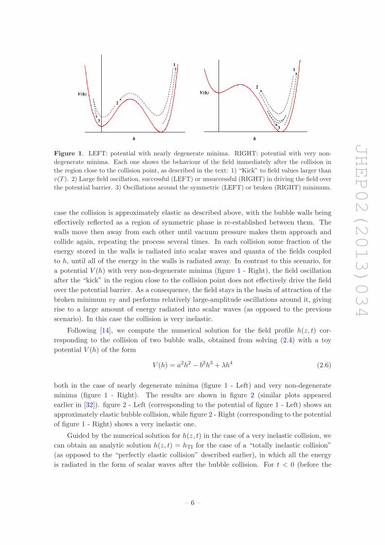
Figure 1. LEFT: potential with nearly degenerate minima. RIGHT: potential with very non-

degenerate minima. Each one shows the behaviour of the field immediately after the collision in

the region close to the collision point, as described in the text: 1) “Kick” to field values larger than

v(T ). 2) Large field oscillation, successful (LEFT) or unsuccessful (RIGHT) in driving the field over

the potential barrier. 3) Oscillations around the symmetric (LEFT) or broken (RIGHT) minimum.

case the collision is approximately elastic as described above, with the bubble walls being

effectively reflected as a region of symmetric phase is re-established between them. The

walls move then away from each other until vacuum pressure makes them approach and

collide again, repeating the process several times. In each collision some fraction of the

energy stored in the walls is radiated into scalar waves and quanta of the fields coupled

to h, until all of the energy in the walls is radiated away. In contrast to this scenario, for

a potential V (h) with very non-degenerate minima (figure 1 - Right), the field oscillation

after the “kick” in the region close to the collision point does not effectively drive the field

over the potential barrier. As a consequence, the field stays in the basin of attraction of the

broken minimum vT and performs relatively large-amplitude oscillations around it, giving

rise to a large amount of energy radiated into scalar waves (as opposed to the previous

scenario). In this case the collision is very inelastic.

Following [14], we compute the numerical solution for the field profile h(z, t) cor-

responding to the collision of two bubble walls, obtained from solving (2.4) with a toy

potential V (h) of the form

V (h) = a2h2 − b2h3 + λh4 (2.6)

both in the case of nearly degenerate minima (figure 1 - Left) and very non-degenerate

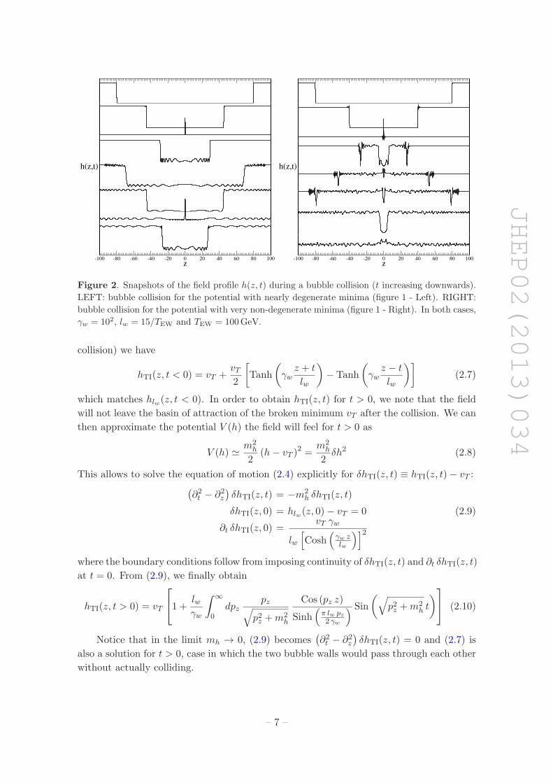
minima (figure 1 - Right). The results are shown in figure 2 (similar plots appeared

earlier in [32]). figure 2 - Left (corresponding to the potential of figure 1 - Left) shows an

approximately elastic bubble collision, while figure 2 - Right (corresponding to the potential

of figure 1 - Right) shows a very inelastic one.

Guided by the numerical solution for h(z, t) in the case of a very inelastic collision, we

can obtain an analytic solution h(z, t) = hTI for the case of a “totally inelastic collision”

(as opposed to the “perfectly elastic collision” described earlier), in which all the energy

is radiated in the form of scalar waves after the bubble collision. For t < 0 (before the

– 6 –

JHEP02(2013)034

-100 -80 -60 -40 -20 0 20 40 60 80 100z

h(z,t)

-100 -80 -60 -40 -20 0 20 40 60 80 100z

h(z,t)

Figure 2. Snapshots of the field profile h(z, t) during a bubble collision (t increasing downwards).

LEFT: bubble collision for the potential with nearly degenerate minima (figure 1 - Left). RIGHT:

bubble collision for the potential with very non-degenerate minima (figure 1 - Right). In both cases,

γw = 102, lw = 15/TEW and TEW = 100GeV.

collision) we have

hTI(z, t < 0) = vT +vT2

[

Tanh

(

γwz + t

lw

)

− Tanh

(

γwz − t

lw

)]

(2.7)

which matches hlw(z, t < 0). In order to obtain hTI(z, t) for t > 0, we note that the field

will not leave the basin of attraction of the broken minimum vT after the collision. We can

then approximate the potential V (h) the field will feel for t > 0 as

V (h) ≃ m2h

2(h− vT )

2 =m2

h

2δh2 (2.8)

This allows to solve the equation of motion (2.4) explicitly for δhTI(z, t) ≡ hTI(z, t)− vT :(

∂2t − ∂2

z

)

δhTI(z, t) = −m2h δhTI(z, t)

δhTI(z, 0) = hlw(z, 0)− vT = 0 (2.9)

∂t δhTI(z, 0) =vT γw

lw

[

Cosh(

γw zlw

)]2

where the boundary conditions follow from imposing continuity of δhTI(z, t) and ∂t δhTI(z, t)

at t = 0. From (2.9), we finally obtain

hTI(z, t > 0) = vT

1 +lwγw

∫ ∞

0dpz

pz√

p2z +m2h

Cos (pz z)

Sinh(

π lw pz2 γw

) Sin

(

√

p2z +m2h t

)

(2.10)

Notice that in the limit mh → 0, (2.9) becomes(

∂2t − ∂2

z

)

δhTI(z, t) = 0 and (2.7) is

also a solution for t > 0, case in which the two bubble walls would pass through each other

without actually colliding.

– 7 –

JHEP02(2013)034

The analysis for the dynamics of bubble collisions presented here may be extended to

phase transitions involving multiple fields (see for example [31]), although in this case the

analysis of the field evolution after the bubble collision becomes much more complicated

(since the scalar potential is multidimensional and the field “excursion” at the moment of

the bubble collision will involve several fields), and we will not attempt it here.

2.2 Particle production through bubble collisions

The bubble collision processes analyzed in the previous section allow to liberate into the

plasma the energy contained in the bubble walls. This can happen either via direct particle

production in the collisions or via radiation of classical scalar waves which will subsequently

decay into particles. For bubble collisions taking place in a thermal environment, the

number densities nα for the different particle species created during the collisions should

very quickly approach the ones in thermal equilibrium nEQα after the phase transition,

thus rendering the particle production process irrelevant for the subsequent evolution of

the Universe. However, as it has been briefly discussed in the introduction, under certain

conditions fast thermalization of certain species after the phase transition may be avoided,

which can make the particle production process very important in that case.

In order to study the particle production through bubble collisions, we will treat the

scalar field configuration h(z, t) as a classical external field and the states coupled to it as

quantum fields in the presence of this source. In doing so, we will neglect the back-reaction

of particle production on the evolution of the bubble walls themselves throughout the

collision, which should be a good approximation when the energy of the produced particles

(for each species) is much less than the energy contained in the field configuration h(z, t).

The probability of particle production is given by [13]

P = 2 Im (Γ [h]) (P ≪ 1) (2.11)

where Γ [h] is the effective action. Γ [h] is the generating functional of 1PI Green functions,

and to the quadratic order in h

Γ [h] =1

2

∫

d4x1 d4x2 h(x1)h(x2) Γ

(2) (x1, x2) (2.12)

with Γ(2) (x1, x2) ≡ Γ(2) (x1 − x2) being the 2-point 1PI Green function. In terms of its

Fourier transform Γ(2)(

p2)

, and using (2.11) and (2.12) we get

P =

∫

d4p

(2π)4Im(

Γ(2)(

p2)

)

∫

d4x1 d4x2 h(x1)h(x2) e

ip(x1−x2) (2.13)

The last integral in (2.13) is just∣

∣

∣h(p)

∣

∣

∣

2, with h(p) being the Fourier transform of the

Higgs field configuration h(x)

h(p) =

∫

d4xh(x) eip x (2.14)

– 8 –

JHEP02(2013)034

For a background field configuration h(z, t), its Fourier transform is given by h(p) =

(2π)2 δ(px) δ(py) h(pz, ω). Then, using (2.13), we obtain the mean number of particles

produced per unit area [13]:

NA

= 2

∫

dpz dω

(2π)2

∣

∣

∣h(pz, ω)

∣

∣

∣

2Im(

Γ(2)(

ω2 − p2z)

)

(2.15)

The physical interpretation of (2.15) is rather simple [13]: the scalar field configuration

h(z, t), corresponding to the two bubble walls that approach and collide, can be decomposed

into modes of definite four-momentum p2 = ω2−p2z via the Fourier transform. Modes with

p2 > 0 represent propagating field quanta with mass squared m2 = p2. Then, (2.15)

integrates over the amount of field quanta of mass p2 contained in the field configuration

multiplied by the probability of those quanta to decay.

The Fourier transform of the background field configuration h(z, t) can be performed

explicitly both for the case of a perfectly elastic collision and of a totally inelastic one

analyzed in the previous section. For a perfectly elastic collision, in the limit of infinitely

thin walls (h(z, t) = h∞), we obtain

h(pz, ω) = h∞(pz, ω) ≡4 vT

ω2 − p2z(2.16)

However, since the highest values of pz and ω available in the field configuration are

naively expected to be of order γw/lw (modes with pz, ω ≫ γw/lw will be exponentially

damped), the integration in (2.15) should in this case be cut-off for pz > γw/lw and

ω > γw/lw. From (2.15) and (2.16) we then obtain

N∞A

=32 v2Tπ2

∫γwlw

0dω

∫γwlw

0dpz

Im(

Γ(2)(

ω2 − p2z)

)

(ω2 − p2z)2 (2.17)

Alternatively, when the thickness of the bubble walls is accounted for (h(z, t) = hlw),

the Fourier transform of (2.3) gives

h(pz, ω) = hlw(pz, ω) ≡π lw ω

2 γw

4 vT

Sinh[

π lw ω2 γw

]

1

ω2 − p2z(2.18)

which automatically incorporates the exponential damping for ω, pz ≫ γw/lw. The mean

number of particles per unit area now reads

Nlw

A=

8 v2T l2wγ2w

∫ ∞

0dω

∫ ∞

0dpz

Im(

Γ(2)(

ω2 − p2z)

)

(ω2 − p2z)2

ω2

(

Sinh[

π lw ω2 γw

])2 (2.19)

For the opposite case of a totally inelastic collision (h(z, t) = hTI), the Fourier trans-

form is given by

h(pz, ω) = hTI(pz, ω) ≡π lw pz2 γw

2 vT

Sinh[

π lw pz2 γw

]

(

1

ω2 − p2z− 1

ω2 − p2z −m2h

)

(2.20)

– 9 –

JHEP02(2013)034

The relative “−” sign between the two contributions in (2.20) can be easily understood

noticing that in the limit mh → 0 the Fourier transform of hTI(z, t) should give h(pz, ω) ∼δ(ω ± pz). From (2.20), the mean number of particles produced per unit area in the case

of a totally inelastic collision is given by

NTI

A=

2 v2T l2wγ2w

∫ ∞

0dω

∫ ∞

0dpz

m4h Im

(

Γ(2)(

ω2 − p2z)

)

(ω2 − p2z)2 (ω2 − p2z −m2

h

)2

p2z(

Sinh[

π lw pz2 γw

])2 (2.21)

The expressions (2.17), (2.19) and (2.21) can be rewritten in a more compact form by

making the change of variables χ = ω2 − p2z, Ψ = ω2 + p2z. After performing the integral in

Ψ, the mean number of particles produced per unit area finally reads

NA

=1

2π2

∫ ∞

0dχ f(χ) Im

(

Γ(2) (χ))

(2.22)

The function f(χ) encodes the details of the bubble collision process and quantifies the

efficiency of particle production. For a perfectly elastic collision, in the limit of infinitely

thin bubble walls, we have

f(χ) = f∞(χ) ≡

16 v2T Log

2(

γwlw

)

2

−χ+2 γwlw

√

(

γwlw

)

2

−χ

χ

χ2Θ

[

(

γwlw

)2

− χ

]

(2.23)

For a perfectly elastic collision, and for bubble walls with finite thickness, we have

f(χ) = flw(χ) ≡2π2 l2w v2T

γ2w

1

χ2

∫ ∞

χdΨ

Ψ+ χ√

Ψ2 − χ2

1(

Sinh[

π lw√Ψ+χ

2√2 γw

])2 (2.24)

Finally, for a totally inelastic collision, we have

f(χ) = fTI(χ) ≡π2 l2w v2T2 γ2w

m4h

χ2(

χ−m2h

)2

∫ ∞

χdΨ

Ψ− χ√

Ψ2 − χ2

1(

Sinh[

π lw√Ψ−χ

2√2 γw

])2 (2.25)

In figure 3 we compare the efficiency f(χ) for the various cases (2.23), (2.24) and (2.25).

Notice that fTI(χ) diverges as χ → m2h. This divergence is artificial, due to considering

h(z, t) over infinite time and space, and should be cut-off since our solution is not valid

over distances larger than the bubble radius RB. Implementing this cut-off can be well

approximated by replacing in (2.24)

(

χ−m2h

)2 →(

χ−m2h

)2+ (m6

h l2w)/γ

2w. (2.26)

Defining χmin as the minimum value of χ for which particle production is possible

(corresponding to the squared sum of the masses Mα of the particles being produced),

we immediately see from figure 3 that for a totally inelastic collision, production of light

particles (χmin < m2h) may be very efficient, while production of heavy particles (χmin ≫

– 10 –

JHEP02(2013)034

0.01 0.1 1 10 100 1000χ

10-5

10-4

10-3

10-2

10-1

100

101

102

103

104

105

106

107

f(χ)

0.01 0.1 1 10 100 1000 10000 100000χ

10-10

10-8

10-6

10-4

10-2

1

102

104

106

108

f(χ)

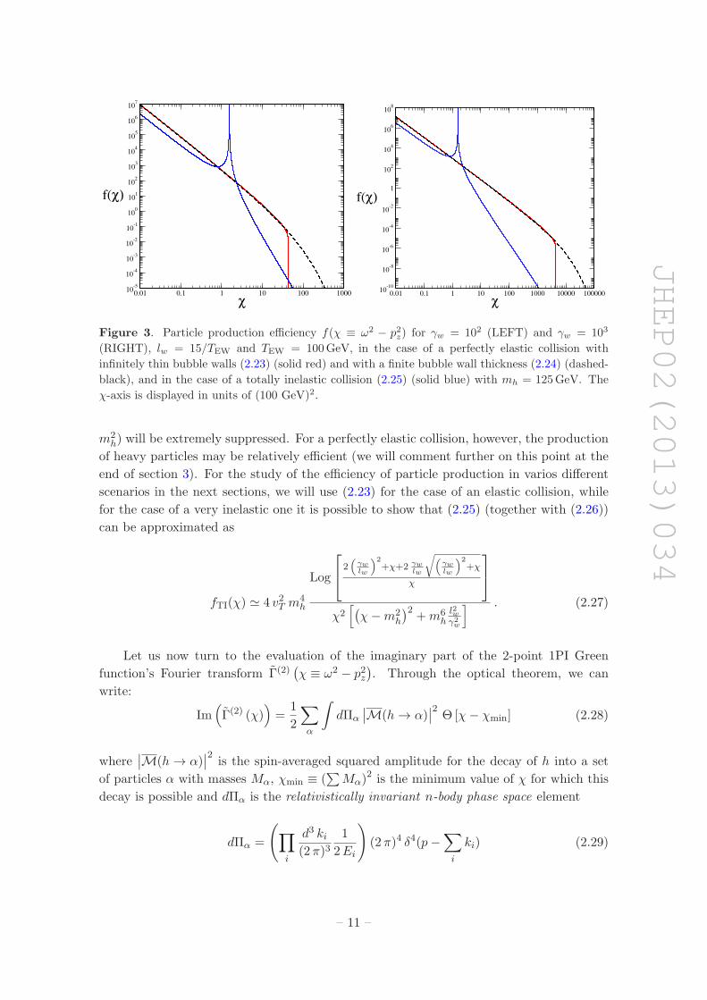
Figure 3. Particle production efficiency f(χ ≡ ω2 − p2z) for γw = 102 (LEFT) and γw = 103

(RIGHT), lw = 15/TEW and TEW = 100GeV, in the case of a perfectly elastic collision with

infinitely thin bubble walls (2.23) (solid red) and with a finite bubble wall thickness (2.24) (dashed-

black), and in the case of a totally inelastic collision (2.25) (solid blue) with mh = 125GeV. The

χ-axis is displayed in units of (100 GeV)2.

m2h) will be extremely suppressed. For a perfectly elastic collision, however, the production

of heavy particles may be relatively efficient (we will comment further on this point at the

end of section 3). For the study of the efficiency of particle production in varios different

scenarios in the next sections, we will use (2.23) for the case of an elastic collision, while

for the case of a very inelastic one it is possible to show that (2.25) (together with (2.26))

can be approximated as

fTI(χ) ≃ 4 v2T m4h

Log

2(

γwlw

)2

+χ+2 γwlw

√

(

γwlw

)2

+χ

χ

χ2[

(

χ−m2h

)2+m6

hl2wγ2w

] . (2.27)

Let us now turn to the evaluation of the imaginary part of the 2-point 1PI Green

function’s Fourier transform Γ(2)(

χ ≡ ω2 − p2z)

. Through the optical theorem, we can

write:

Im(

Γ(2) (χ))

=1

2

∑

α

∫

dΠα

∣

∣M(h → α)∣

∣

2Θ [χ− χmin] (2.28)

where∣

∣M(h → α)∣

∣

2is the spin-averaged squared amplitude for the decay of h into a set

of particles α with masses Mα, χmin ≡ (∑

Mα)2 is the minimum value of χ for which this

decay is possible and dΠα is the relativistically invariant n-body phase space element

dΠα =

(

∏

i

d3 ki(2π)3

1

2Ei

)

(2π)4 δ4(p−∑

i

ki) (2.29)

– 11 –

JHEP02(2013)034

Then, the number of particles of a certain type α produced per unit area during the

bubble collision will simply read from (2.22) and (2.28)

NA

∣

∣

∣

∣

α

=1

4π2

∫ ∞

χmin

dχ f(χ)

∫

dΠα

∣

∣M(h → α)∣

∣

2(2.30)

The amount of energy produced per unit area in the form of particles α is obtained by

weighting (2.30) by the energy of each decaying Fourier mode. This yields

EA

∣

∣

∣

∣

α

=1

4π2

∫ ∞

χmin

dχ f(χ)√χ

∫

dΠα

∣

∣M(h → α)∣

∣

2(2.31)

From (2.30) and (2.31), the non-thermally produced energy density ρα (assuming that

the produced particles quickly diffuse into the bubble interior) reads

ρα ≡ EV

∣

∣

∣

∣

α

=EA

∣

∣

∣

∣

α

A

V≃ E

A

∣

∣

∣

∣

α

3

2RB(2.32)

with A ∼ 4π R2B being the total collision area and V the volume of the two colliding

bubbles. From (2.32), and bearing in mind that RB ≃ β−1, the non-thermally generated

comoving energy density is

Υα =ρα

s(TEW)≃ 20√

π g∗

1

MPl TEW

β

H

EA

∣

∣

∣

∣

α

(2.33)

with s(TEW) the entropy density after the EW phase transition.

3 Particle production via the Higgs portal

The efficiency of particle production may strongly depend on the nature of the particles

being produced. In this section we will analyze the particle production efficiency for scalars

S, fermions f and vector bosons Vµ coupled to the Higgs field. Apart from estimating the

production of SM fermions and gauge bosons through this process, we will consider a simple

Higgs-portal extension of the SM in order to study the production of other possible scalar,

fermion or vector boson particles. Furthermore, we will restrict ourselves to Z2 symmetric

Higgs-portal scenarios, since we will ultimately be interested in dark matter analyses. We

also comment on how to interpret the results in the case when the calculated particle

production exceeds the energy available in the bubble wall.

3.1 Scalars

For the complex scalar S interacting with the SM via the Higgs portal, the relevant part

of the lagrangian is given by

−∆Ls = m2s |S|2 + λs |H|2 |S|2 with H =

(

0h+vT√

2

)

. (3.1)

– 12 –

JHEP02(2013)034

1 10 102

103

104

MS (GeV)

10-6

10-5

10-4

10-3

10-2

10-1

1

101

λ = 1λ = 0.1

Υ /Υ

SS

X WMAP

1 10 102

103

104

MS (GeV)

10-5

10-4

10-3

10-2

10-1

1

101

102

103

104

105

λ = 1λ = 0.1

Υ /Υ

S

SX WMAP

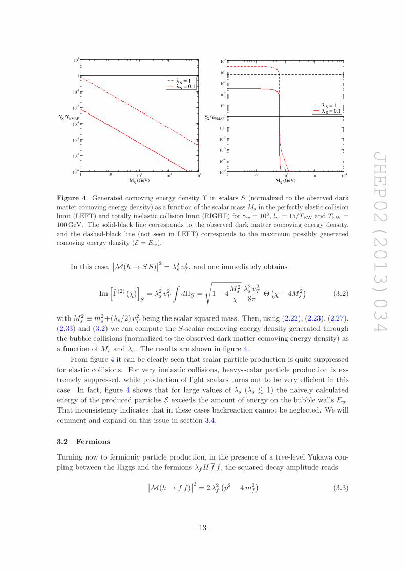
Figure 4. Generated comoving energy density Υ in scalars S (normalized to the observed dark

matter comoving energy density) as a function of the scalar mass Ms in the perfectly elastic collision

limit (LEFT) and totally inelastic collision limit (RIGHT) for γw = 108, lw = 15/TEW and TEW =

100GeV. The solid-black line corresponds to the observed dark matter comoving energy density,

and the dashed-black line (not seen in LEFT) corresponds to the maximum possibly generated

comoving energy density (E = Ew).

In this case,∣

∣M(h → S S)∣

∣

2= λ2

s v2T , and one immediately obtains

Im[

Γ(2) (χ)]

S= λ2

s v2T

∫

dΠS =

√

1− 4M2

s

χ

λ2s v

2T

8πΘ(

χ− 4M2s

)

(3.2)

withM2s ≡ m2

s+(λs/2) v2T being the scalar squared mass. Then, using (2.22), (2.23), (2.27),

(2.33) and (3.2) we can compute the S-scalar comoving energy density generated through

the bubble collisions (normalized to the observed dark matter comoving energy density) as

a function of Ms and λs. The results are shown in figure 4.

From figure 4 it can be clearly seen that scalar particle production is quite suppressed

for elastic collisions. For very inelastic collisions, heavy-scalar particle production is ex-

tremely suppressed, while production of light scalars turns out to be very efficient in this

case. In fact, figure 4 shows that for large values of λs (λs . 1) the naively calculated

energy of the produced particles E exceeds the amount of energy on the bubble walls Ew.

That inconsistency indicates that in these cases backreaction cannot be neglected. We will

comment and expand on this issue in section 3.4.

3.2 Fermions

Turning now to fermionic particle production, in the presence of a tree-level Yukawa cou-

pling between the Higgs and the fermions λfH f f , the squared decay amplitude reads

∣

∣M(h → f f)∣

∣

2= 2λ2

f

(

p2 − 4m2f

)

(3.3)

– 13 –

JHEP02(2013)034

which, in the case of SM fermions, leads directly to

Im[

Γ(2) (χ)]

f=

m2f

4π v2Tχ

(

1−4m2

f

χ

)3

2

Θ(

χ− 4m2f

)

(3.4)

The production of (SM) fermions will then be enhanced with respect to the one of

Higgs-portal S−scalars (specially in the limit of very elastic collisions, see figure 5) due to

the extra factor(

χ− 4m2f

)

in (3.4). Scenarios where the fermionic particle production

might be important include (apart from the SM itself) the MSSM and its various extensions,

due to the tree-level coupling between Higgses, Higgsinos and Gauginos.5

In the absence of a direct coupling, the interaction between the Higgs and the fermions

will occur via an effective operator. This is the case for the so-called fermionic Higgs-portal:

−∆Lf = mf ff +λf

Λ|H|2 ff (3.5)

However, since bubble collisions may excite very massive Higgs field modes (p2 ≫T 2EW), particle production in this case may be sensitive to the UV completion of the Higgs-

portal effective theory, making it unreliable to compute the particle production in the

fermionic Higgs-portal via (3.5). Here we consider a simple UV completion for the fermionic

Higgs-portal, and compute the particle production in this case. We add a singlet scalar

field S as a mediator between the Higgs field and the fermion f , the relevant part of the

lagrangian being

−∆Lf =m2

s

2S2 +

λs

2|H|2 S2 + µs |H|2 S +mf ff + λfS ff (3.6)

For simplicity, we will avoid a vev for S (it can be done through the addition of a linear

term for S in (3.6)). For µs 6= 0 the effective fermionic Higgs-portal operator |H|2 ff will

be generated at tree-level. The squared decay amplitude for h → f f will then be

∣

∣M(h → f f)∣

∣

2= 2

λ2f µ

2s v

2T

(p2 −M2s )

2 + Γ2s M

2s

(

p2 − 4m2f

)

(3.7)

with

Γs =λ2s v

2T + µ2

s

16πMs

√

1− 4m2h

M2s

Θ(

M2s − 4m2

h

)

+λ2f Ms

8π

(

1−4m2

f

M2s

)3

2

Θ(

M2s − 4m2

f

)

(3.8)

leading finally to

Im[

Γ(2) (χ)]

f=

λ2f µ

2s v

2T

4π

χ

(χ−M2s )

2 + Γ2s M

2s

(

1−4m2

f

χ

)3

2

Θ(

χ− 4m2f

)

(3.9)

5In particular, the production of neutralino dark matter might have an impact on the subsequent evo-

lution of the Universe.

– 14 –

JHEP02(2013)034

1 10 102

103

104

mf (GeV)

10-6

10-4

10-2

1

102

104

λ = 0.1λ = 1λ = λ = 1λ = λ = 1

Υ /Υ

ff

s

Top Production

f

f s

X WMAP

1 10 102

103

104

mf (GeV)

10-6

10-5

10-4

10-3

10-2

10-1

1

101

102

103

104

105

λ = 0.1λ = 1λ = λ = 1λ = λ = 1

Υ /Υf

f

s

Top Production

ff

s

X WMAP

Figure 5. Generated comoving energy density Υ in fermions f (normalized to the observed dark

matter comoving energy density) as a function of the fermion mass mf in the perfectly elastic

collision limit (LEFT) and totally inelastic collision limit (RIGHT) for γw = 108, lw = 15/TEW

and TEW = 100GeV. Red lines: production in the presence of a direct tree-level Yukawa coupling

between fermions and Higgs (3.4). Blue lines: production for a tree-level effective coupling (3.9),

for µs = Ms = 500GeV (solid) and 5TeV (dashed). Yellow lines: production for a 1-loop effective

coupling (3.10). The solid-black line corresponds to the observed dark matter comoving energy

density, and the dashed-black line corresponds to the maximum possible generated comoving number

density (E = Ew).

When µs = 0 the effective fermionic Higgs-portal operator is not generated at tree-

level, but rather the decay h → f f occurs via a finite 1-loop diagram, yielding

Im[

Γ(2) (χ)]

f=

(

λs λ2f

)2

(4π)5F[

m2f , M

2s , χ

]

χ

(

1−4m2

f

χ

)3

2

Θ(

χ− 4m2f

)

(3.10)

where F[

m2f , M

2s , χ

]

is a form factor that scales as

F[

m2f , M

2s , χ

]

−→m4

f

χ2Log

(

χ

m2f

)

χ ≫ m2f , M

2s (3.11)

Fermionic Higgs-portal particle production both in the µs = 0 and µs 6= 0 is shown in

figure 5, where it can be clearly seen that the production in the absence of a direct coupling

between the Higgs and the fermions f differs from what would have been naively obtained

using (3.5). As for the case of scalar particle production, under certain circumstances the

estimate of fermionic particle production neglecting backreaction exceeds the amount of

energy stored in the bubble walls (E > Ew), and in order to obtain a physically meaningful

result backreaction should be included (We will expand on this issue in section 3.4).

3.3 Vector bosons

Finally, we study the production of vector boson particles. In the presence of a tree-

level coupling between the Higgs and the vector bosons λV MV hVµVµ, the squared decay

– 15 –

JHEP02(2013)034

amplitude reads∣

∣M(h → Vµ Vµ)∣

∣

2= λ2

V M2V

(

3− p2

M2V

+p4

4M4V

)

(3.12)

leading to

Im[

Γ(2) (χ)]

V=

λ2V M

2V

8π

(

3− χ

M2V

+χ2

4M4V

)

√

1− 4M2

V

χΘ(

χ− 4M2V

)

(3.13)

Comparing (3.2), (3.4) and (3.13) we immediately observe the relative efficiency of

particle production for scalars, fermions and vector bosons. While Im [Γ(2) (χ)] scales as χ0

for scalars, and as χ for fermions, in the case of vector bosons it scales as χ2, thus greatly

enhancing production of vector bosons with respect to scalars or fermions for very elastic

collisions (see figure 6). It is then expected that most of the available energy from the

EW phase transition will go into Wµ and Zµ gauge boson production and (possibly) other

vector bosons coupled at tree-level to the Higgs in extensions of the SM.6

In the absence of a direct coupling, the interaction between the Higgs and the vector

bosons may occur via an effective operator, as in the so-called vector Higgs-portal [34]:

−∆LV =1

2m2

V VµVµ + λV |H|2 VµV

µ (3.14)

However (like for the fermionic Higgs-portal) an analysis of vector boson particle pro-

duction in the context of the effective theory (3.14) will be unreliable due to very massive

Higgs field modes (p2 ≫ T 2EW) being excited during the bubble collisions. Vector boson par-

ticle production will then be sensitive to the way in which the effective operator |H|2 VµVµ

is generated. One possible way of generating the effective operator at tree-level, being Vµ a

hidden U(1) gauge field, is by integrating out a U(1)-charged complex scalar S which has

a Higgs portal coupling |H|2 S∗S, the relevant part of the lagrangian then being

−∆LV =1

4FµνF

µν −DµS∗DµS + V (S) + λhs |H|2 S∗S (3.15)

In this scenario, the vector boson Vµ acquires a mass via the spontaneous breaking

of the hidden U(1), through a vev vS for the S-scalar.7 The squared decay amplitude for

h → Vµ Vµ will then be

∣

∣M(h → Vµ Vµ)∣

∣

2=

λ2hs

4

v2T M4V

(p2 −M2s )

2 + Γ2s M

2s

(

3− p2

M2V

+p4

4M4V

)

(3.16)

with Γs being the decay width of S. This leads to

Im[

Γ(2) (χ)]

V=

λ2hs

32π

v2T M4V

(

3− χM2

V

+ χ2

4M4

V

)

(χ−M2s )

2 + Γ2s M

2s

√

1− 4M2V

χΘ(

χ− 4M2V

)

(3.17)

6Such as Little Higgs theories or extra-dimensional scenarios with gauge fields living in the bulk.7This implies that there may have been another phase transition in the early Universe associated with

the spontaneous breaking of the hidden U(1) gauge symmetry, which we need to require to have happened

long before the EW phase transition since otherwise the EW phase transition would have been effectively

multi-field and our present analysis of particle production would be totally unrealistic.

– 16 –

JHEP02(2013)034

1 10 102

103

104

MV (GeV)

10-3

1

103

106

109

1012

1015

1018

λ = 0.1λ = 0.1

Υ /Υ

W Boson Production

Z Boson Production

X WMAP

V

V

1 10 102

103

104

MV (GeV)

10-6

10-5

10-4

10-3

10-2

10-1

1

101

102

103

104

105

106

λ = 0.1λ = 0.1

Υ /Υ

Z Boson Production

W Boson Production

X WMAP

V

V

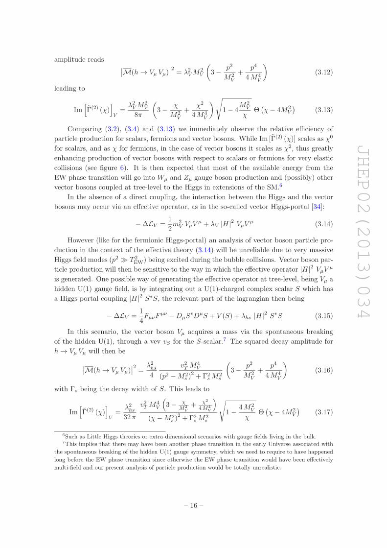
Figure 6. Generated comoving energy density Υ in vector bosons Vµ (normalized to the observed

dark matter comoving energy density) as a function of the vector boson mass MV in the per-

fectly elastic collision limit (LEFT) and totally inelastic collision limit (RIGHT) for γw = 108,

lw = 15/TEW and TEW = 100GeV. Red line: production in the presence of a direct tree-level

coupling between vector bosons and Higgs (3.13). Blue line: production for a tree-level effective

coupling (3.17), for λhs = 1 and Ms = 500GeV. The solid-black line corresponds to the observed

dark matter comoving energy density, and the dashed-black line corresponds to the maximum

possible generated comoving number density (E = Ew).

Vector boson effective Higgs-portal particle production is shown in figure 6, resulting

in a very suppressed particle production with respect to the case in which the vector

bosons and the Higgs couple directly at tree-level, specially for very elastic collisions. From

figure 6 it is also clear that backreaction is most important for direct vector boson particle

production (for which the production estimate yields E ≫ Ew).

3.4 Backreaction and relative efficiency

Clearly, for the present analysis of particle production to be physically meaningful it must

be assumed that the total energy of the produced particles is less than the energy contained

in the background field configuration h(z, t). Moreover, when the energy of the produced

particles starts being comparable to the energy of the background field we expect backre-

action on h(z, t) due to the particle production to be important. Then, in order for the

previous analysis to be reliable, it is needed

EA

∣

∣

∣

∣

X

≪ Ew

A=

2

3v2T

γwlw

(3.18)

As it has been shown in the previous section, for fermion or vector boson particle

production the previous condition (3.18) is not satisfied, and in some cases even E ≫ Ew

is obtained (figure 6 LEFT), signaling the extreme importance of backreaction in those

scenarios.

Since incorporating backreaction into the present analysis of particle production is

extremely difficult and lies beyond the scope of this paper, we simply note that the relative

– 17 –

JHEP02(2013)034

10 102

103

104

MX (GeV)

10-12

10-11

10-10

10-9

10-8

10-7

10-6

10-5

10-4

10-3

10-2

10-1

100

Eff

icie

ncy

λ = 0.1λ = 0.5λ = 1

V

V

f

10 102

103

104

MX (GeV)

10-12

10-11

10-10

10-9

10-8

10-7

10-6

10-5

10-4

10-3

10-2

10-1

100

Eff

icie

ncy

λ = 0.1λ = 0.5V

V

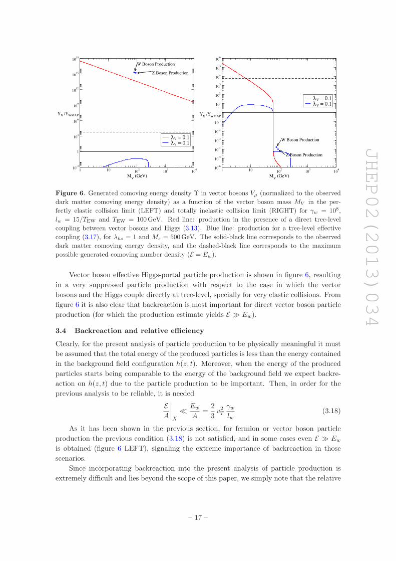
Figure 7. Efficiency of vector boson (solid lines) and fermion (dashed line) particle production

(scalars are too inefficiently produced to be shown) for a perfectly elastic collision, normalized to

the most efficiently produced particles (in this case Wµ and Zµ) and to the energy contained in the

bubble walls, for γw = 108 (LEFT) and γw = 1015 (RIGHT), lw = 15/TEW and TEW = 100GeV.

The solid-black line corresponds to the observed dark matter comoving energy density (normalized

to the energy contained in the bubble walls).

efficiency in particle production for the different species in the present analysis should be

roughly correct even when backreaction is important. Then, an estimate of the particle

production in cases where some of the species are very efficiently produced may be obtained

just by normalizing the production to the total energy in the bubble walls. For very elastic

bubble collisions, it has been shown in section 3.3 that production of Wµ and Zµ gauge

bosons is extremely efficient, which will then leave very little energy left in the bubble walls

for producing other particle species. The relative efficiencies (defined as ratios of energy

in produced particles) of the different species for a perfectly elastic collision, normalized to

the energy contained in the bubble walls (assuming that most of the available energy goes

into producing Wµ and Zµ) is shown in figure 7. A good estimate of the non-thermally

generated comoving energy density (per particle species α) in this case may then be given by

Υα ≃ 20√π g∗

1

MPl TEW

β

H

EA

∣

∣

∣

∣

α

(

EA

∣

∣

∣

∣

Wµ

)−1Ew

A(3.19)

The fact that this is a reliable estimate of the particle production efficiency for the case

of very elastic collisions is due to the high-p2 modes of the bubble wall carrying almost all

the energy of the bubble wall. The energy carried by the high-p2 modes will then mostly

go into vector boson production (their production efficiency at high p2 is much larger than

fermionic or scalar ones), result that holds even without incorporating backreaction into

the analysis.

– 18 –

JHEP02(2013)034

On the other hand, for very inelastic collisions the results from the previous section

show that particle production is only effective for light particles (MX . mh/2). Therefore,

production of Wµ and Zµ will be very suppressed in this case, along with any other heavy

particle, and most of the available energy will go into production of SM fermions (mainly

bottom quarks) and (possibly) new light scalars or fermions with sizable couplings to

the Higgs.

4 Non-thermal multi-TeV WIMP dark matter

In this section we focus on the case of relatively heavy dark matter, MX &TeV, and ex-

plore the conditions under which the amount of non-thermally produced heavy dark matter

can end-up accounting for a sizable part of the observed dark matter relic density (dark

matter may nevertheless still have a thermal component coming from the usual freeze-out

process). The first condition is clearly that bubble collisions have to be fairly elastic: it has

been shown in sections 3 that for very inelastic bubble collisions only light (MX . mh/2)

particles are efficiently produced, while heavy particle production is extremely suppressed.

Since fast thermalization of light species after the EW phase transition seems unavoidable,8

for very inelastic bubble collisions either dark matter is not efficiently produced or it ther-

malizes immediately after the end of the EW phase transition, not having any influence on

the subsequent evolution of the Universe.

For very elastic bubble collisions, the analysis from sections 3 and 3.4 shows that elec-

troweak gauge bosons Wµ and Zµ are most efficiently produced, and the relative production

efficiency of heavy fermions and scalars is too low (for them to be able to account for a

sizable part of the observed dark matter relic abundance, see figure 7). This leaves heavy

vector bosons with a direct coupling to the Higgs field as the only viable candidate for

non-thermally produced dark matter during the EW phase transition.

In the following we perform an analysis of heavy vector boson dark matter coupled

to the Higgs, including an overview of thermal freeze-out and direct detection constrains

from XENON100 [33] (see [34, 35] for more details), and a comparison between the amount

of non-thermally produced dark matter and the amount of dark matter produced through

thermal freeze-out. We also study the evolution of the non-thermally produced dark matter

component after the EW phase transition.

4.1 Higgs-vector dark matter interplay

Consider a vector boson dark matter candidate with mass MV and a tree-level coupling to

the Higgs [34, 36, 37],

LV =1

2M2

V VµVµ + λV vThVµVµ (4.1)

This coupling mediates the dark matter annihilation into Standard Model particles, as

well as the elastic scattering on nucleons relevant for dark matter direct detection. Con-

cerning the former process, the Higgs boson can mediate annihilation of dark matter into

8Dark matter may be coupled to the Higgs weakly enough as to avoid thermalization, however in that

case we find it is not produced in sufficient quantities to make up for the observed relic abundance. For a

discussion of the asymmetric dark matter case, see apppendix A.

– 19 –

JHEP02(2013)034

electroweak gauge bosons (for heavy dark matter they are the most important annihilation

channel) through the couplings

h

vT

(

2M2WW+

µ W−µ +M2

ZZµZµ

)

(4.2)

The spin-averaged amplitude squared for the annihilation process VµVµ → W+µ W−

µ in

the limit s ≫ m2h is given by

|MV V→W/Z,W/Z |2 ≈2

3λ2V

(

s2

4M4V

− s

M2V

+ 3

)

(4.3)

Given (4.3), the thermally averaged annihilation cross section is given by

〈σv〉V V→W/Z,W/Z =z λ2

V

192πM2V K2(z)2

∫ ∞

4dx

√x− 4K1(

√x z)

(

x(x− 4)

4+ 3

)

(4.4)

where z = MV /T , and K1(z),K2(z) are Bessel functions. For z ≫ 1, (4.4) reduces to

〈σv〉V V→W/Z,W/Z ≈ λ2V

16πM2V

(4.5)

The thermal cross section giving rise to the observed value of the relic density

〈σv〉WMAP ≈ 2.6 · 10−9GeV−2 corresponds, for heavy dark matter MV ≫ mh and us-

ing (4.5), to[

λV

MV (TeV)

]

WMAP

≈ 0.3 (4.6)

Turning now to dark matter direct detection, the spin-averaged amplitude squared for

Higgs-mediated dark matter elastic scattering on nucleons reads

|MV N→V N |2 = 8λ2V f2

N m2N

3 (t−m2h)

2

(

2 +(M2

V − t2)

M2V

)(

2m2N − t

2

)

≈ 16λ2V f2

N m4N

m4h

(4.7)

Here, mN ≈ 0.939GeV is the proton/neutron mass and fN is the effective Yukawa coupling

of the Higgs to nucleons which, following [35], we take fN = 0.326 based on the lattice

estimate in [38] (see also [39]). In the last step we have taken the limit t ≪ m2N ,m2

h,M2V .

The elastic scattering cross section then reads

σV N→V N ≈ λ2V f2

N m4N

πM2V m4

h

≈ 4.2 · 10−44cm2

[

λV

MV (TeV)

]2

(4.8)

On the other hand, the XENON100 bound on the dark matter elastic scattering cross

section on nucleons, for MV &TeV is approximately

σV N→V N < MV · 2.2 · 10−44cm2 (4.9)

Therefore, (4.6) and (4.9) leave a sizable window in the parameter space (MV , λV ) for

which the dark matter abundance obtained via thermal freeze-out is significantly smaller

than the observed dark matter relic density, and still the value of λV (as a function of MV )

is below the XENON100 bound (as shown in figure 8).

– 20 –

JHEP02(2013)034

500 1000 2000 3000 5000 10000M

V (GeV)

0.1

1

10

λ50 %25 %10 %V

Thermal DM Abundance Larger

than DM Relic Abundance

Excluded by XENON100

Figure 8. The dashed-black line corresponds to the limits on λV from XENON100 (4.9). The

solid-black line corresponds to the value of λV for which the observed DM relic density is obtained

via thermal freeze-out (4.6): below it the thermal DM density is larger than the observed DM relic

density (and thus this region is excluded). Above, the thermal DM density is only a fraction of the

observed DM relic density, and the red lines show the percentage of relic density accounted for by

the thermal density.

4.2 Fate of non-thermally produced vector dark matter

Given the results from the previous section (summarized in figure 8), it is fair to ask if, in

the region of (MV , λV ) parameter space in which the thermal component is not enough to

account for the observed dark matter relic density, dark matter produced non-thermally at

the EW phase transition could account for the extra needed amount. Using the results from

production efficiency of heavy vector boson dark matter obtained in sections 3.3 and 3.4, we

show in figure 9 the value of λV (as a function of MV ) for which the amount of non-thermal

vector boson production equals the observed dark matter relic density (dashed-blue line).

Then, for values of λV above the thermal cross section giving the observed relic density

〈σ v〉WMAP, non-thermal production of heavy vector bosons is so efficient as to generate

amounts of dark matter much larger than the observed dark matter relic density.

Assuming that at the time of the EW phase transition vector boson dark matter is

already frozen-out (Tfo ≃ MV /20 > TEW), we can study the evolution of the non-thermally

generated dark matter abundance via a simple Boltzmann equation in which the comoving

dark matter number density Y fulfills Y (z) ≫ YEQ(z) (with YEQ(z) being the equilibrium

comoving number density), yielding

dY

dz= −α

〈σ v〉MPlMV

z2Y (z)2 −→ dy

dz= − 1

z2y2(z) (4.10)

with α = (4π2√ξ g∗)/45 ≃ 2.642 (g∗ ∼ 100 being the number of relativistic degrees of

freedom in the thermal plasma and ξ ≡ 90/(32π3)), MPl = 1.2 × 1019GeV and y(z) =

– 21 –

JHEP02(2013)034

500 1000 2000 3000 5000 10000M

V (GeV)

0.1

1

10

λ

TEW = 100 GeV

TEW = 50 GeV

TEW = 30 GeV

V

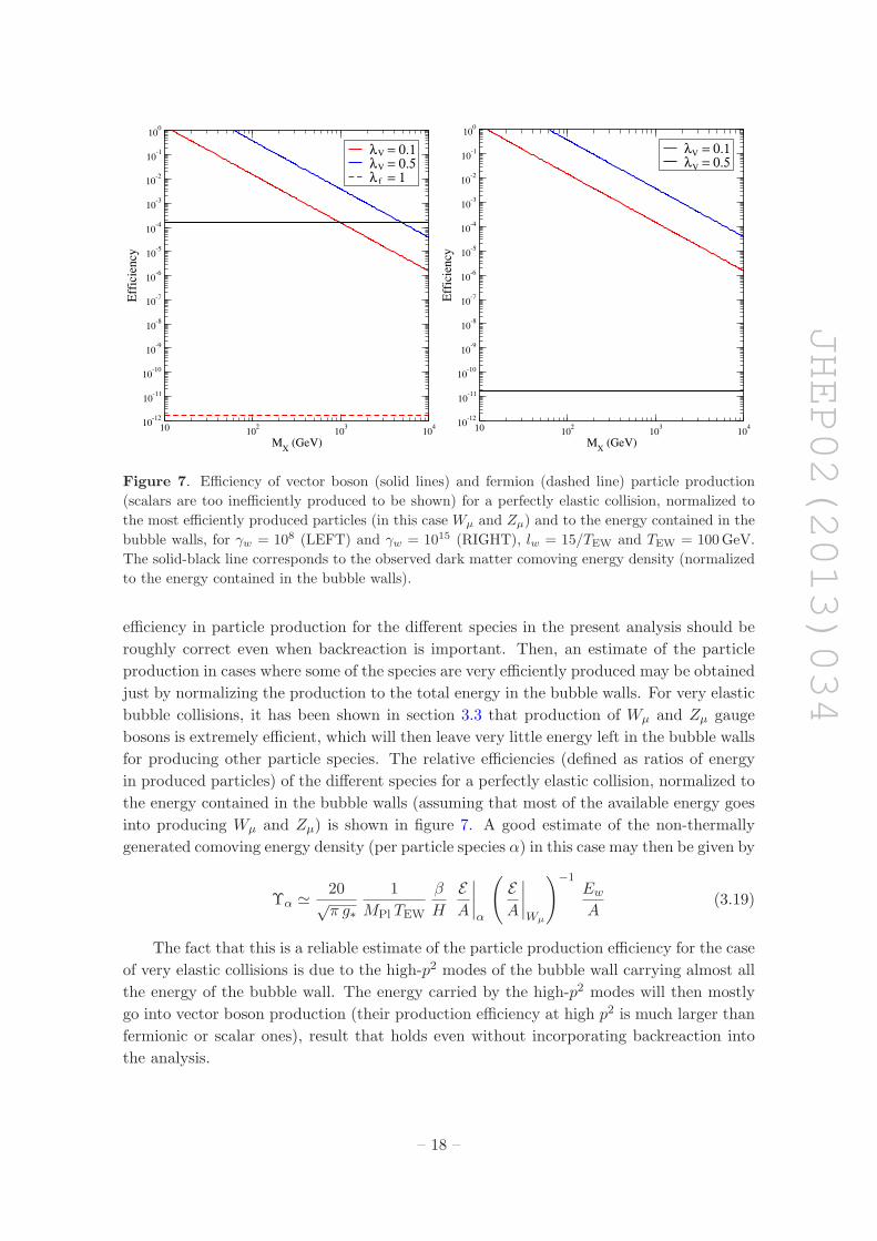
Figure 9. Black lines are the same as in figure 8. The dashed-blue line corresponds to the value of

λV needed for the non-thermally produced energy density in vector bosons (with a direct coupling

to the Higgs) to be equal to the DM relic density, for γw = 108. The red lines show the values of λV

yielding the “non-thermal” cross section (4.13) (for which the final dark matter abundance, taking

into account its evolution after non-thermal production, corresponds to the observed dark matter

relic density) for several values of TEW.

α 〈σ v〉MPlMV Y (z). Integration of (4.10) for z > zEW yields

1

y(z)− 1

y(zEW)=

1

zEW− 1

z−→ 1

y(∞)=

1

zEW+

1

y(zEW)(4.11)

Then, given the fact that non-thermal vector boson dark matter production is much

larger than the observed relic density in the (MV , λV ) region of interest, we can take the

limit y(∞) ≪ y(zEW), obtaining

y(∞) ≃ zEW (4.12)

From (4.12), we immediately obtain that the value of the annihilation cross section

that will yield the observed dark matter relic density once the non-thermally generated

dark matter evolves after the EW phase transition is simply given by

〈σ v〉 = 〈σ v〉WMAP

Tfo

TEW(4.13)

The red lines in figure 9 show the values of λV yielding the correct “non-thermal”

annihilation cross section (4.13) for several values of TEW.

This analysis shows that non-thermal production of multi-TeV vector boson dark mat-

ter at the EW phase transition (in (MV , λV ) parameter space in which the amount of dark

matter yielded by thermal freeze-out is not enough to account for the observed dark matter

relic density) is efficient as to generate a dark matter amount much larger than the observed

relic density. This results in a reactivation of thermalization processes that lead to partial

– 22 –

JHEP02(2013)034

104

105

106

107

108

MV (GeV)

10-3

10-2

10-1

1

λV

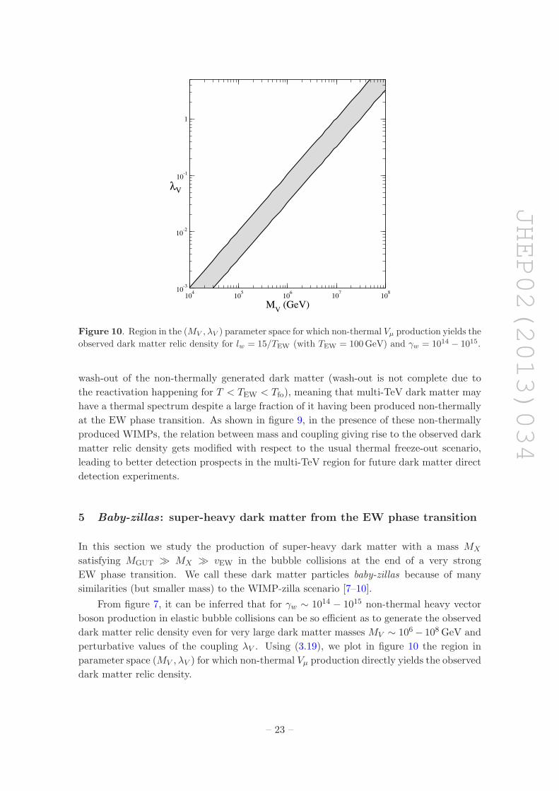
Figure 10. Region in the (MV , λV ) parameter space for which non-thermal Vµ production yields the

observed dark matter relic density for lw = 15/TEW (with TEW = 100GeV) and γw = 1014 − 1015.

wash-out of the non-thermally generated dark matter (wash-out is not complete due to

the reactivation happening for T < TEW < Tfo), meaning that multi-TeV dark matter may

have a thermal spectrum despite a large fraction of it having been produced non-thermally

at the EW phase transition. As shown in figure 9, in the presence of these non-thermally

produced WIMPs, the relation between mass and coupling giving rise to the observed dark

matter relic density gets modified with respect to the usual thermal freeze-out scenario,

leading to better detection prospects in the multi-TeV region for future dark matter direct

detection experiments.

5 Baby-zillas: super-heavy dark matter from the EW phase transition

In this section we study the production of super-heavy dark matter with a mass MX

satisfying MGUT ≫ MX ≫ vEW in the bubble collisions at the end of a very strong

EW phase transition. We call these dark matter particles baby-zillas because of many

similarities (but smaller mass) to the WIMP-zilla scenario [7–10].

From figure 7, it can be inferred that for γw ∼ 1014 − 1015 non-thermal heavy vector

boson production in elastic bubble collisions can be so efficient as to generate the observed

dark matter relic density even for very large dark matter masses MV ∼ 106 − 108GeV and

perturbative values of the coupling λV . Using (3.19), we plot in figure 10 the region in

parameter space (MV , λV ) for which non-thermal Vµ production directly yields the observed

dark matter relic density.

– 23 –

JHEP02(2013)034

104

105

106

107

108

MV (GeV)

103

104

105

106

107

TRH

(GeV)

Figure 11. Bounds on the Reheating temperature after inflation for the requirement that dark

matter never reaches thermal equilibrium after inflation, namely TRH ≤ Tfo, as a function of the

dark matter massMV , and assuming λV (MV ) for which non-thermal production yields the observed

relic abundance (as shown in figure 10).

5.1 Bounds on the reheating temperature after inflation

A stable particle with mass MV ∼ 105−108GeV would yield a much larger relic abundance

than the observed DM relic density. were it in thermal equilibrium at some stage after

inflation. For such a massive species, the annihilation cross is always smaller than the one

needed to yield the observed DM relic density through thermal freeze-out. It is then needed

that this particle species never reached thermal equilibrium after the end of inflation. This

sets an upper bound on the reheating temperature after inflation, specifically TRH < Tfo

(with Tfo being the temperature below which the particle is decoupled from the thermal

plasma). For a heavy vector boson Vµ annihilating into SU(2) gauge bosons (the most

important annihilation channel in this case) through the Higgs, Tfo satifies

MV

Tfo≃ 20.4 + Log

(

MV

100GeV

)

+ Log

( 〈σv〉10−9GeV−2

)

(5.1)

where the thermally averaged annihilation cross section 〈σv〉 is given by (4.4). In figure 11

we plot the minimum value of z (corresponding to the maximum allowed value of the

reheating temperature TRH) as a function of the mass MV for the range of λV values giving

rise to the observed dark matter relic abundance for γw = 1014 − 1015 (see figure 10). We

see that the upper bound on TRH is relatively insensitive to the precise value of γw, and

roughly scales as TmaxRH ∼ MV /10.

– 24 –

JHEP02(2013)034

6 Conclusions

Dark matter may have been efficiently produced at the end of a first order EW phase

transition if it has a large coupling to the Higgs field. In this paper we investigated the

conditions for this non-thermal production mechanism to account for most of dark matter

in the Universe. We considered scalar, fermion and vector dark matter coupled to the SM

through the Higgs (either via a direct, tree-level interaction or an effective Higgs-portal

coupling), and found that production of vector bosons directly coupled to the Higgs is

most efficient, while for scalar and fermions most of the energy stored in the bubble walls

is bound to be released into production of SM particles. This analysis singles out vector

dark matter in the present context.

For very inelastic bubble collisions only dark with MX . 100GeV can be efficiently

produced, while production of heavier dark matter is extremely suppressed. Unfortunately,

for a dark matter mass in this range, we did not find a way to avoid subsequent thermal-

ization and the wash-out of the non-thermal component, and therefore in this case dark

matter production at the EW phase transition is irrelevant. The situation is quite different

for highly elastic bubble collisions. In that case, dark matter with MX ≫ 100GeV can

be efficiently produced for the so-called runaway bubbles, that expand with a very large

γ-factor.

We have identified two scenarios where wash-out of dark matter produced at the EW

phase transition can be naturally avoided. One has dark matter in the multi-TeV range,

which makes it possible for non-thermally produced dark matter to remain out of thermal

equilibrium after the EW phase transition. We determined the region in the parameter

space of dark matter mass and coupling to the Higgs where the correct relic abundance

is reproduced. For a given mass, the coupling has to be larger than in the usual thermal

freeze-out scenario for Higgs portal dark matter, which can be especially relevant for direct

detection searches, as it opens the possibility of detecting a signal from multi-TeV non-

thermal dark matter in the near future by XENON100 and LUX experiments. The other

scenario is baby-zilla dark matter with MX ∼ 106-108GeV. Surprisingly enough, such

super-heavy dark matter can be produced in important quantities at the end of a strongly

first-order EW phase transition, provided the dark matter coupling to the Higgs is large,

and the γ factor of the bubble walls is near its maximal value of γw ∼ 1015. In order

for the baby-zillas to be a viable dark matter candidate, they must have never reached

thermal equilibrium, which then constrains the reheating temperature after inflation in

this scenario.

Acknowledgments

We specially thank Francesco Riva for very useful discussions and collaboration in the

early stages of this work, and also Thomas Konstandin, Michel Tytgat, Yann Mambrini,

Stephan Huber and Stephen West for discussions and comments. The work of J.M.N. is

supported by the Science Technology and Facilities Council (STFC) under grant number

ST/J000477/1.

– 25 –

JHEP02(2013)034

A Asymmetric dark matter production

We now explore the possibility of asymmetric dark matter production during the EW

phase transition, together with the viability of this mechanism as a way to avoid wash-out

of non-thermal production for relatively light dark matter (and any other light species in

general).

For multi-component dark matter (X = Xα), an asymmetry in the number densities

of Xα and Xα may be generated during the particle production. We will analyze in detail

below the generation of this asymmetry for scalars (Xα = Sα). Then, in section A.2 we

study the evolution of the generated asymmetries after the EW phase transition.

A.1 Decay asymmetries: producing a dark matter asymmetry

Let us consider a set of Ni real scalars hi (that includes the field(s) involved in the EW

phase transition) coupled to a set of Nα complex scalars Sα via a trilinear interaction. The

relevant part of the lagrangian is

−∆L = m2α S

∗αSα + Ciαβ hi S

∗αSβ + V (hi) (A.1)

where by hermiticity Ciαβ = C∗iβα (it follows that Ciαα are real, but Ciαβ with α 6= β

can be complex), and the mass matrix for the scalars Sα is taken to be diagonal without

loss of generality. We also consider a possible term µij hi h2j appearing in V (hi). The

lagrangian (A.1) incorporates a Z2 symmetry that makes the lightest of the scalars Sα

stable, which may then be a suitable dark matter candidate. In order for an asymmetry in

the production of Sα and S∗α to be generated, we need a nonzero value for

|M(hi → S∗α Sβ)|2 −

∣

∣M(hi → S∗β Sα)

∣

∣

2(A.2)

At tree level

MTree(hi → S∗α Sβ) = Ciαβ

MTree(hi → S∗β Sα) = C∗

iαβ

⇒ |M(hi → S∗α Sβ)|2 =

∣

∣M(hi → S∗β Sα)

∣

∣

2= |Ciαβ |2

(A.3)

and there is no asymmetry generated. At 1-loop we include the 1PI diagrams shown in

figure 12. Their contribution to the 1-loop decay amplitude is

M1L(hi → S∗α Sβ) = − 1

16π2

∑

j,γ,δ

(

CiγδCjαγCjδβ IT + µijCjαδCjδβ IT

)

M1L(hi → S∗β Sα) = − 1

16π2

∑

j,γ,δ

(

C∗iγδC

∗jαγC

∗jδβ IT + µijC

∗jαδC

∗jδβ IT

)

(A.4)

where the integrals IT and IT correspond to

IT =−i

π2

∫

d4k1

(k2 −m2γ)((k + p)2 −m2

δ)((k − k2)2 −m2j )

IT =−i

π2

∫

d4k1

(k2 −m2j )((k + p)2 −m2

j )((k − k2)2 −m2δ)

(A.5)

– 26 –

JHEP02(2013)034

hihi hi

hj

hj

hj

Sα

Sβ

Sα

Sβ

Sγ

Sδ

Sα

Sδ

Sβ

***

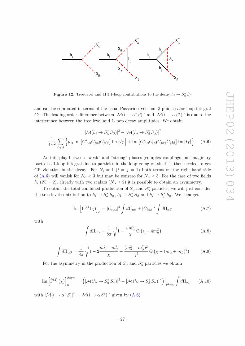
Figure 12. Tree-level and 1PI 1-loop contributions to the decay hi → S∗

α Sβ

and can be computed in terms of the usual Passarino-Veltman 3-point scalar loop integral

C0. The leading order difference between |M(i → α∗ β)|2 and |M(i → αβ∗)|2 is due to the

interference between the tree level and 1-loop decay amplitudes. We obtain

|M(hi → S∗α Sβ)|2 −

∣

∣M(hi → S∗β Sα)

∣

∣

2=

1

4π2

∑

j,γ,δ

µij Im[

C∗iαβCjαδCjδβ

]

Im[

IT

]

+ Im[

C∗iαβCiγδCjαγCjδβ

]

Im [IT ]

(A.6)

An interplay between “weak” and “strong” phases (complex couplings and imaginary

part of a 1-loop integral due to particles in the loop going on-shell) is then needed to get

CP violation in the decay. For Ni = 1 (i = j = 1) both terms on the right-hand side

of (A.6) will vanish for Nα < 3 but may be zonzero for Nα ≥ 3. For the case of two fields

hi (Ni = 2), already with two scalars (Nα ≥ 2) it is possible to obtain an asymmetry.

To obtain the total combined production of Sα and S∗α particles, we will just consider

the tree level contribution to hi → S∗α Sα, hi → S∗

α Sβ and hi → S∗β Sα. We then get

Im[

Γ(2) (χ)]

α= |Ciαα|2

∫

dΠαα + |Ciαβ |2∫

dΠαβ (A.7)

with∫

dΠαα =1

8π

√

1− 4m2α

χΘ(

χ− 4m2α

)

(A.8)

∫

dΠαβ =1

8π

√

1− 2m2

α +m2β

χ+

(m2α −m2

β)2

χ2Θ(

χ− (mα +mβ)2)

(A.9)

For the asymmetry in the production of Sα and S∗α particles we obtain

Im[

Γ(2) (χ)]Asym

α=(

|M(hi → S∗α Sβ)|2 −

∣

∣M(hi → S∗β Sα)

∣

∣

2)∣

∣

∣

p2=χ

∫

dΠαβ (A.10)

with |M(i → α∗ β)|2 − |M(i → αβ∗)|2 given by (A.6).

– 27 –

JHEP02(2013)034

A.2 Fate of the generated asymmetric abundance

The asymmetric dark matter production process outlined in the previous section will generi-

cally result in asymmetries for the comoving number densities for particles and antiparticles

of the different species ∆α ≡ YXα − YX∗

α6= 0 at the end of the EW phase transition. Note

however that the Z2 symmetry forces the sum of the asymmetries of the different species

Xα to vanish∑

α

∆α = 0 (A.11)

After the EW phase transition, the comoving number densities for the different species

YXα will evolve according to a system of coupled Boltzmann equations. Denoting the sym-

metric and asymmetric part of the comoving number densities for particles and antiparticles

of the different species by Ξα ≡ YXα + YX∗

αand ∆α, we can write

z H(z)dΞα

dz= −s

2〈σ v〉α+α∗→SM

[

Ξ2α −∆2

α −(

ΞEqα

)2]

−s

2

∑

β 6=α

〈σ v〉α+β∗→SM

[

ΞαΞβ −∆α∆β − ΞEqα ΞEq

β

]

−∑

β 6=α

〈σ v〉α+SM→β+SM

[

Ξα − ΞEqα Ξβ

ΞEqβ

]

−∑

β 6=α

Γα→β+SM

[

Ξα − ΞEqα Ξβ

ΞEqβ

]

(A.12)

z H(z)d∆α

dz= −s

2

∑

β 6=α

〈σ v〉α+β∗→SM [∆αΞβ − Ξα∆β ]

−∑

β 6=α

〈σ v〉α+SM→β+SM

[

∆α − ΞEqα ∆β

ΞEqβ

]

−∑

β 6=α

Γα→β+SM

[

∆α − ΞEqα ∆β

ΞEqβ

]

(A.13)

where s is the entropy density, z = mL/T (mL is the mass of the lightest species Xα) and

H(z) is the Hubble parameter. From (A.12), if the annihilation processes are unsuppressed

the symmetric comoving number densities for the various species Xα will be driven close

to thermal equilibrium (the small departure from equilibrium being due to the presence of

an asymmetry ∆α)

Ξα →√

∆2α +

(

ΞEqα

)2(A.14)

Ideally, in the absence of wash-out of ∆α, these processes would delay freeze-out and

still be active for ∆α ≫ ΞEqα , annihilating away the symmetric part of the number density

and leading to Ξα → ∆α. However, the various processes entering (A.13) will tend to erase

the asymmetries ∆α. In particular, the process Xα + SM → Xβ + SM (responsible for

kinetic equilibrium among the different species Xα) and the decay process Xα → Xβ +

SM, will, if active, wash-out the asymmetries very rapidly, being also quite insensitive to

– 28 –

JHEP02(2013)034

the temperature of the Universe after the EW phase transition (the annihilation process

Xα +X∗β → SM also washes-out the asymmetries, but is suppressed for low TEW). If these

processes are in equilibrium after the EW phase transition, they will very rapidly drive

∆α →∑

β 6=α

∆β (A.15)

which, together with (A.11), leads to ∆α → 0. While it is possible for the decay process

Xα → Xβ + SM to be suppressed if the different species are quite degenerate, this auto-

matically results in unsuppressed kinetic equilibrium. This seems to rule-out asymmetric

production as a viable mechanism to avoid complete wash-out of the amount of light dark

matter non-thermally produced during the EW phase transition, the reason being that it

is not possible (at least in this simple scenario) to keep all the processes that tend to erase

the asymmetries ∆α out of equilibrium after the EW phase transition, while having an

efficient particle production at the transition itself.

Open Access. This article is distributed under the terms of the Creative Commons

Attribution License which permits any use, distribution and reproduction in any medium,

provided the original author(s) and source are credited.

References

[1] WMAP collaboration, E. Komatsu et al., Seven-Year Wilkinson Microwave Anisotropy

Probe (WMAP) Observations: Cosmological Interpretation,

Astrophys. J. Suppl. 192 (2011) 18 [arXiv:1001.4538] [INSPIRE].

[2] S. Dodelson and L.M. Widrow, Sterile-neutrinos as dark matter,

Phys. Rev. Lett. 72 (1994) 17 [hep-ph/9303287] [INSPIRE].

[3] J. Preskill, M.B. Wise and F. Wilczek, Cosmology of the Invisible Axion,

Phys. Lett. B 120 (1983) 127 [INSPIRE].

[4] L. Abbott and P. Sikivie, A Cosmological Bound on the Invisible Axion,

Phys. Lett. B 120 (1983) 133 [INSPIRE].

[5] M. Dine and W. Fischler, The Not So Harmless Axion, Phys. Lett. B 120 (1983) 137

[INSPIRE].

[6] T. Moroi and L. Randall, Wino cold dark matter from anomaly mediated SUSY breaking,

Nucl. Phys. B 570 (2000) 455 [hep-ph/9906527] [INSPIRE].

[7] D.J. Chung, E.W. Kolb and A. Riotto, Nonthermal supermassive dark matter,

Phys. Rev. Lett. 81 (1998) 4048 [hep-ph/9805473] [INSPIRE].

[8] D.J. Chung, E.W. Kolb and A. Riotto, Superheavy dark matter,

Phys. Rev. D 59 (1999) 023501 [hep-ph/9802238] [INSPIRE].

[9] D.J. Chung, E.W. Kolb and A. Riotto, Production of massive particles during reheating,

Phys. Rev. D 60 (1999) 063504 [hep-ph/9809453] [INSPIRE].

[10] E.W. Kolb, D.J. Chung and A. Riotto, WIMPzillas!, hep-ph/9810361 [INSPIRE].

[11] T. Konstandin and G. Servant, Cosmological Consequences of Nearly Conformal Dynamics

at the TeV scale, JCAP 12 (2011) 009 [arXiv:1104.4791] [INSPIRE].

– 29 –

JHEP02(2013)034

[12] S. Hawking, I. Moss and J. Stewart, Bubble Collisions in the Very Early Universe,

Phys. Rev. D 26 (1982) 2681 [INSPIRE].

[13] R. Watkins and L.M. Widrow, Aspects of reheating in first order inflation,

Nucl. Phys. B 374 (1992) 446 [INSPIRE].

[14] T. Konstandin and G. Servant, Natural Cold Baryogenesis from Strongly Interacting

Electroweak Symmetry Breaking, JCAP 07 (2011) 024 [arXiv:1104.4793] [INSPIRE].

[15] S.Y. Khlebnikov, Fluctuation - dissipation formula for bubble wall velocity,

Phys. Rev. D 46 (1992) 3223 [INSPIRE].

[16] P.B. Arnold, One loop fluctuation - dissipation formula for bubble wall velocity,

Phys. Rev. D 48 (1993) 1539 [hep-ph/9302258] [INSPIRE].

[17] G.D. Moore and T. Prokopec, How fast can the wall move? A Study of the electroweak phase

transition dynamics, Phys. Rev. D 52 (1995) 7182 [hep-ph/9506475] [INSPIRE].

[18] G.D. Moore, Electroweak bubble wall friction: Analytic results, JHEP 03 (2000) 006

[hep-ph/0001274] [INSPIRE].

[19] P. John and M. Schmidt, Do stops slow down electroweak bubble walls?,

Nucl. Phys. B 598 (2001) 291 [Erratum ibid. B 648 (2003) 449] [hep-ph/0002050]

[INSPIRE].

[20] P.J. Steinhardt, Relativistic detonation waves and bubble growth in false vacuum decay,

Phys. Rev. D 25 (1982) 2074 [INSPIRE].

[21] M. Gyulassy, K. Kajantie, H. Kurki-Suonio and L.D. McLerran, Deflagrations and

Detonations as a Mechanism of Hadron Bubble Growth in Supercooled Quark Gluon Plasma,

Nucl. Phys. B 237 (1984) 477 [INSPIRE].

[22] H. Kurki-Suonio, Deflagration bubbles in the quark - hadron phase transition,

Nucl. Phys. B 255 (1985) 231 [INSPIRE].

[23] K. Kajantie and H. Kurki-Suonio, Bubble Growth and Droplet Decay in the Quark Hadron

Phase Transition in the Early Universe, Phys. Rev. D 34 (1986) 1719 [INSPIRE].

[24] M. Laine, Bubble growth as a detonation, Phys. Rev. D 49 (1994) 3847 [hep-ph/9309242]

[INSPIRE].

[25] H. Kurki-Suonio and M. Laine, Supersonic deflagrations in cosmological phase transitions,

Phys. Rev. D 51 (1995) 5431 [hep-ph/9501216] [INSPIRE].

[26] J.R. Espinosa, T. Konstandin, J.M. No and G. Servant, Energy Budget of Cosmological

First-order Phase Transitions, JCAP 06 (2010) 028 [arXiv:1004.4187] [INSPIRE].

[27] M. Kamionkowski, A. Kosowsky and M.S. Turner, Gravitational radiation from first order

phase transitions, Phys. Rev. D 49 (1994) 2837 [astro-ph/9310044] [INSPIRE].

[28] D. Bodeker and G.D. Moore, Can electroweak bubble walls run away?, JCAP 05 (2009) 009

[arXiv:0903.4099] [INSPIRE].

[29] T. Konstandin and J.M. No, Hydrodynamic obstruction to bubble expansion,

JCAP 02 (2011) 008 [arXiv:1011.3735] [INSPIRE].

[30] C. Hogan, Nucleation of cosmological phase transitions, Phys. Lett. B 133 (1983) 172

[INSPIRE].

– 30 –

JHEP02(2013)034

[31] J. Giblin, John T., L. Hui, E.A. Lim and I.-S. Yang, How to Run Through Walls: Dynamics

of Bubble and Soliton Collisions, Phys. Rev. D 82 (2010) 045019 [arXiv:1005.3493]

[INSPIRE].

[32] Joy Division, Unknown Pleasures, Factory Records (1979).

[33] XENON100 collaboration, E. Aprile et al., Dark Matter Results from 225 Live Days of

XENON100 Data, Phys. Rev. Lett. 109 (2012) 181301 [arXiv:1207.5988] [INSPIRE].

[34] O. Lebedev, H.M. Lee and Y. Mambrini, Vector Higgs-portal dark matter and the invisible

Higgs, Phys. Lett. B 707 (2012) 570 [arXiv:1111.4482] [INSPIRE].

[35] A. Djouadi, O. Lebedev, Y. Mambrini and J. Quevillon, Implications of LHC searches for

Higgs–portal dark matter, Phys. Lett. B 709 (2012) 65 [arXiv:1112.3299] [INSPIRE].

[36] T. Hambye and M.H. Tytgat, Confined hidden vector dark matter,

Phys. Lett. B 683 (2010) 39 [arXiv:0907.1007] [INSPIRE].

[37] S. Kanemura, S. Matsumoto, T. Nabeshima and N. Okada, Can WIMP Dark Matter

overcome the Nightmare Scenario?, Phys. Rev. D 82 (2010) 055026 [arXiv:1005.5651]

[INSPIRE].

[38] R. Young and A. Thomas, Octet baryon masses and sigma terms from an SU(3) chiral

extrapolation, Phys. Rev. D 81 (2010) 014503 [arXiv:0901.3310] [INSPIRE].

[39] J. Martin Camalich, L. Geng and M. Vicente Vacas, The lowest-lying baryon masses in

covariant SU(3)-flavor chiral perturbation theory, Phys. Rev. D 82 (2010) 074504

[arXiv:1003.1929] [INSPIRE].

– 31 –