published for sissa by springer2010)159.pdf · published for sissa by springer received: july 28,...
TRANSCRIPT
JHEP11(2010)159
Published for SISSA by Springer
Received: July 28, 2010
Revised: September 27, 2010
Accepted: November 16, 2010
Published: November 30, 2010
Bounds and decays of new heavy vector-like top
partners
Giacomo Cacciapaglia,a Aldo Deandrea,a Daisuke Haradab,c and Yasuhiro Okadab,c
aUniversite de Lyon, France; Universite Lyon 1,CNRS/IN2P3, UMR5822 IPNL, F-69622 Villeurbanne Cedex, FrancebKEK Theory Center, Institute of Particle and Nuclear Studies, KEK,1-1 Oho, Tsukuba, Ibaraki 305-0801, JapancDepartment of Particle and Nuclear Physics,Graduate University for Advanced Studies (Sokendai),1-1 Oho, Tsukuba, Ibaraki 305-0801, Japan
E-mail: [email protected], [email protected],[email protected], [email protected]
Abstract: We study the phenomenology of new heavy vector-like fermions that couple tothe third generation quarks via Yukawa interactions, covering all the allowed representa-tions under the standard model gauge groups. We first review tree and loop level boundson these states. We then discuss tree level decays and loop-induced decays to photon orgluon plus top. The main decays at tree level are to Wb and/or Z and Higgs plus top viathe new Yukawa couplings. The radiative loop decays turn out to be quite close to thenaive estimate: in all cases, in the allowed perturbative parameter space, the branchingratios are mildly sensitive on the new Yukawa couplings and small. We therefore concludethat the new states can be observed at the LHC and that the tree level decays can allow todistinguish the different representations. Moreover, the observation of the radiative decaysat the LHC would suggest a large Yukawa coupling in the non-perturbative regime.
Keywords: Beyond Standard Model, Heavy Quark Physics
ArXiv ePrint: 1007.2933
Open Access doi:10.1007/JHEP11(2010)159
JHEP11(2010)159
Contents
1 Introduction 1
2 The effective model 22.1 Two fermion mixing 3
3 Third generation quarks 53.1 Case I: singlets 73.2 Case II: SM doublet 83.3 Case III: non-SM doublets 93.4 Case IVa: triplet 2
3 103.5 Case IVb: triplet −1
3 11
4 Tree level and radiative decays 12
5 Numerical results 13
6 Conclusions 16
A General loop calculation formulas 19
B Decay width formulas 25B.1 A quick estimate 25B.2 Decay widths and the the large mass limit 26
1 Introduction
In many models of new physics, like for example extra dimensional models, Little Higgsmodels, dynamical models, there are heavy vector-like fermions which decay to StandardModel (SM) fermions plus a boson (W/Z and/or Higgs h). Moreover the mixing of vector-like quarks with the third generation and in particular the top quark is a common featurein little Higgs models [1–4] and composite Higgs models based on top condensation ([5–8];for recent bounds see [9]). We are at present at the beginning of the Large Hadron Collider(LHC) era which is an exciting time for discovery of new particles and test of models nearthe electroweak scale. Previous collider and precision data place however limits on newheavy quarks and set the lowest mass scale for these resonances once some properties forthese particles are assumed. Direct searches give mass constraints in the range of 200-300 GeV, typically assuming a charged current decay chain ([10] and 2009 partial updatefor the 2010 edition). Precision tests can be stringent in some cases but more modeldependent as the effect of new particles or couplings may affect the precision observables
– 1 –
JHEP11(2010)159
in both directions. Indeed in the past vector fermion models were for example suggested toimprove the Rb data at LEP2 [11–13]. More recently it was proposed that the discrepancyof the measured asymmetry AFBb with the standard model can be reduced through theintroduction of new quarks with non-trivial mixings with the third generation [14]. Mixingeffects with the SM quarks give stringent bounds in the case of mixing with the first twogenerations but only mild bounds for the mixing with the third generation. For a discussionof the parametrisation of mixing effects and CP bounds see [15]. In the following we shallfocus on vector-like quarks in various representations for which a coupling to a standardHiggs doublet is possible. We will assume that there is only one fermion that couples tothe third generation of quarks, the top and bottom, via a Yukawa coupling. This situationcan reproduce with a good accuracy models where only the top partners are lighter thanother heavy fermions like, for example, composite Higgs models [16]. This case is in generaldifferent from the case of a chiral fourth generation, for which more stringent bounds canbe obtained [17–19].
In order to keep the discussion general we will not consider any specific model butrather an effective approach where the decays are induced by a new Yukawa coupling.This coupling generates the mixing of the new heavy fermion with top and bottom. Wewill ignore the possible mixing to the light generations which is strongly constrained byflavour physics. The idea is to study tree level and radiative decays (loop induced decayinto photon or gluon plus SM fermion) due to such Yukawa interactions to understandif the observation of such modes at the LHC would allow us to distinguish the differentcases and/or estimate the size of the new Yukawa couplings. In the next section, we willdefine the effective model, and study the possible Yukawa interactions as a function ofthe representation of the heavy fermion and the number of new fermions. In section 3 welimit ourselves to the third generation of quarks and define the allowed parameter space.In section 4 we present the results for the tree and loop level decays and in section 5 wediscuss the numerical results and briefly the LHC prospects.
2 The effective model
In the following we shall assume that the new fermions interact with the SM fermions viaYukawa interactions. The quantum numbers of the new fermions with respect to the weakSU(2)L× U(1)Y gauge group are therefore limited by the requirement of an interaction withthe Higgs doublet and one of the SM fermions. The standard model contains a doubletqL = {uL, dL} = (2, Y ) and two singlets uR = (1, Y + 1
2) and dR = (1, Y − 12) where Y = 1
6
for quarks and Y = 12 for leptons, and the Higgs H = (2, 1
2). The SM Yukawa couplings are:
LYuk = −yu qLHcuR − yd qLHdR + h.c. , (2.1)
Taking into account the quantum numbers of the standard model particles one can easilycheck the possible quantum number assignments for the new fermions. One can add anew singlet fermion with the same hypercharge assignments as in the SM, namely Y ± 1
2 .There are 3 possible doublets: one with the SM hypercharge Y , and two others with Y ±1.Finally, one can add two triplets with hypercharge Y ± 1
2 .
– 2 –
JHEP11(2010)159
In the following we will denote by U and D the heavy partners of the up and downSM particles, namely the states that will mix with the SM fermions. We will denote bya X the eventual extra fermion that does not mix with SM ones, because of a differentelectric charge.
2.1 Two fermion mixing
The Yukawa coupling λ connecting the heavy fermions with the SM ones will generatea mixing between the two states, with the light one to be identified with the SM masseigenstate. In general, there are two types of mixing: the singlets and triplets couple tothe left-handed doublet, while the doublets couple with the right-handed singlets. In thefollowing we will study these two cases in general, adding two heavy states, U and D, andparametrising their mixing with the SM states. This formalism can then easily adapted tothe different representations of the heavy fermions.
In the case of singlets and triplets, after the Higgs doublet develops a vacuum expec-tation value
〈H〉 =
(0v+h√
2
), (2.2)
where v ∼ 246 GeV and h is the physical Higgs boson, the mass terms will look like
Lmass = −yuv√2uLuR − x uLUR −M ULUR + h.c. , (2.3)
where x ∼ λv with the proportionality factor depending on the representation U belongsto (a similar expression holds for down-type fermions). In the singlet case, a mass termULuR is also allowed, however one can always find a combination of UR and uR to removesuch parameter and redefine the Yukawa couplings.
The mass matrix can be diagonalised by two mixing matrices
V L,Ru =
(cos θL,Ru sin θL,Ru
− sin θL,Ru cos θL,Ru
), (2.4)
defined as (cos θLu − sin θLusin θLu cos θLu
)(yuv√
2x
0 M
)(cos θRu sin θRu− sin θRu cos θRu
)=
(mt 00 mt′
), (2.5)
where mt′ ≥ M ≥ mt. The relations between the three input parameters and the mixingangles and masses can be expressed as
y2uv
2
2= m2
t
(1 +
x2
M2 −m2t
), (2.6)
m2t′ = M2
(1 +
x2
M2 −m2t
), (2.7)
sin θLu =Mx√
(M2 −m2t )2 +M2x2
, (2.8)
sin θRu =mt
Msin θLu . (2.9)
– 3 –
JHEP11(2010)159
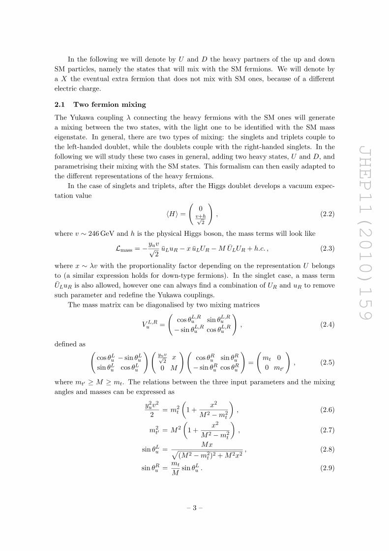
200 400 600 800 1000m_t'
200
400
600
800
1000M
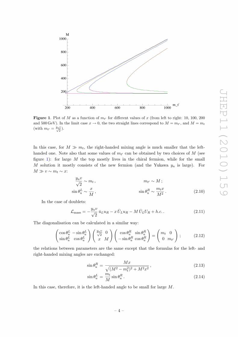
Figure 1. Plot of M as a function of mt′ for different values of x (from left to right: 10, 100, 200and 500 GeV). In the limit case x→ 0, the two straight lines correspond to M = mt′ , and M = mt
(with mt′ = yuv√2
).
In this case, for M � mt, the right-handed mixing angle is much smaller that the left-handed one. Note also that some values of mt′ can be obtained by two choices of M (seefigure 1): for large M the top mostly lives in the chiral fermion, while for the smallM solution it mostly consists of the new fermion (and the Yukawa yu is large). ForM � v ∼ mt ∼ x:
yuv√2∼ mt , mt′ ∼M ;
sin θLu ∼x
M, sin θRu ∼
mtx
M2. (2.10)
In the case of doublets:
Lmass = −yuv√2uLuR − x ULuR −M ULUR + h.c. . (2.11)
The diagonalisation can be calculated in a similar way:(cos θLu − sin θLusin θLu cos θLu
)(yuv√
20
x M
)(cos θRu sin θRu− sin θRu cos θRu
)=
(mt 00 mt′
); (2.12)
the relations between parameters are the same except that the formulas for the left- andright-handed mixing angles are exchanged:
sin θRu =Mx√
(M2 −m2t )2 +M2x2
, (2.13)
sin θLu =mt
Msin θRu . (2.14)
In this case, therefore, it is the left-handed angle to be small for large M .
– 4 –

JHEP11(2010)159
Using the mixing matrices, we can express the couplings to Z, W and h as two bytwo matrices in the mass eigenstate basis (the couplings with the photon and gluon staydiagonal due to gauge invariance). If we denote by gsmW and gψW the couplings of the Wwith the SM doublet and the new fermion respectively, the left-handed couplings can bewritten as:
gWL =(V Ld
)† ·( gsmW 00 gψW
)· V L
u =
(gsmW cLd c
Lu + gψW s
Ld s
Lu g
smW cLd s
Lu − g
ψW s
Ld cLu
gsmW sLd cLu − g
ψW c
Ld s
Lu g
smW sLd s
Lu + gψW c
Ld cLu
), (2.15)
where s and c stand for the sin and cos of the mixing angles. The same formula applies forthe right-handed couplings, with gsmW = 0:
gWR =(V Rd
)† ·( 0 00 gψW
)· V R
u =
(gψW s
Rd s
Ru −g
ψW s
Rd c
Ru
−gψW cRd sRu gψW cRd c
Ru
). (2.16)
Note that gsmW = g√2, and gψW , the same for left- and right-handed components, depends on
the representation: it is equal to the SM one for a doublet and equal to ±g for a triplet.Note also that in the case where either U or D are absent, the same formulas can be usedjust setting gψW = 0 and setting to zero the absent mixing angle. Similarly, a general matrixformula can be written for the Z couplings of both left- and right-handed ups and downs:
gZf = (Vf )† ·
(gsmZ 00 gψZ
)· Vf =
(gsmZ c2 + gψZs
2 (gsmZ − gψZ)sc
(gsmZ − gψZ)sc gsmZ s2 + gψZc
2
). (2.17)
Note here that the Z couplings can be always expressed as function of the weak isospinand charge of the fermion:
gZ(T3, Y ) =g
cos θW
(T3 − sin2 θWQ
). (2.18)
Finally, we can express the Higgs couplings in the two cases as:
λh =(V L)† ·( y√
2xv
0 0
)· V R =
cL(cR y√
2− sR xv
)cL(sR y√
2+ cR xv
)sL(cR y√
2− sR xv
)sL(sR y√
2+ cR xv
) , (2.19)
λh =(V L)† ·( y√
20
xv 0
)· V R =
cR(cL y√
2− sL xv
)sR(cL y√
2− sL xv
)cR(sL y√
2+ cL xv
)sR(sL y√
2+ cL xv
) . (2.20)
3 Third generation quarks
Precision tests on new vector-like fermions play an important role to constrain the possiblerange of masses, couplings and mixings. For light quarks and leptons, the modification oftree level couplings to the gauge bosons poses a very strong bound on the masses or mixingangles, therefore we will ignore this case. The only case that may be relevant for the LHCis a mixing in the third generation of quarks: in the following we will consider only mixinginvolving top and bottom quarks, and assume that the mixing effects are negligible for thelight generations so that they do not appear in flavour measurements.
– 5 –
JHEP11(2010)159
Nevertheless, tree level bounds, typically coming from W → tb or Z → bb due to mixingeffects with the new heavy fermions, give important indications: they are “robust” bounds,in the sense that they only depend on the mixing parameter and the properties of the newparticle. Loop-level bounds, as for example oblique corrections, are also an important andoften stringent test of the possible range of parameters for new heavy fermions, howeverthey are more model dependent than the previous ones. In fact, heavier particles thatappear in a specific model also contribute leading to potential cancellations. Moreover, theHiggs mass is still unmeasured and its variation from the reference value can compensatefor the heavy fermion contributions. The importance of the oblique corrections is due to thefact that in many extensions of the Standard Model the vacuum-polarisation diagrams arethe main corrections to the standard particle interactions. However the oblique correctionsare not much useful if the new particles mix strongly with the standard ones as in this casedirect corrections to the standard particle will be much more important [20, 21]. We willconsider both type of direct and oblique corrections in the following.
The direct bound to the coupling of the W to top and bottom is coming from theobservation of single top production at TeVatron: we will allow a variation of ±20% [22, 23].A tighter constraint originates from the unitarity of the CKM mixing matrix and flavourphysics: however such bound is not applicable here because it does not take into accountthe effect of the heavy fermions, and it is also sensible to the contribution of other particlesin the model (see [24] for a detailed study of bounds for singlet quarks and [25] for avector-like up-type quark or a fourth generation). The couplings of the Z to the bottomare also directly measured and very constrained [26]: in the left-handed coupling a +1%and −0.2% deviations are allowed; in the right-handed one, +20% and −5%. In the casesunder study, only one of the two is affected, so that those limits are sufficient even thoughthe bounds are correlated; in the case where they are both present, a more detailed fitis required.
For the oblique corrections, we calculated the contribution to the T parameter [27]. Adetailed study is given in [28, 29]. We allow for a deviation of +0.4 and −0.2: we consider atighter bound on negative values because it is generically more difficult to accommodate fora negative shift in T . For instance, increasing the Higgs mass with respect to the referencevalue will generate an effective negative contribution. This is a very conservative boundand we use it just to underline the power of oblique constraints with respect to the treelevel ones. As mentioned above, model dependent contribution from other heavier particlesmay be relevant and give rise to cancellation, therefore significantly modifying the allowedparameter space.
Another important bound on the parameter space comes from direct searches at theTeVatron. The most recent bounds are 335 GeV for a t′ state ([30]; and a previous note [31]),and 385 GeV for a b′ ([32]; and a previous paper [33]): however, those bounds assume 100%branching ratios t′ → Wq and b′ → Wt. This is true for a fourth generation, but in ourcase decays in neutral bosons will play an important role. Case by case, we will set a boundroughly at the Zt or ht thresholds, where the branching ratio in W ’s will become muchsmaller than 100% .
– 6 –
JHEP11(2010)159
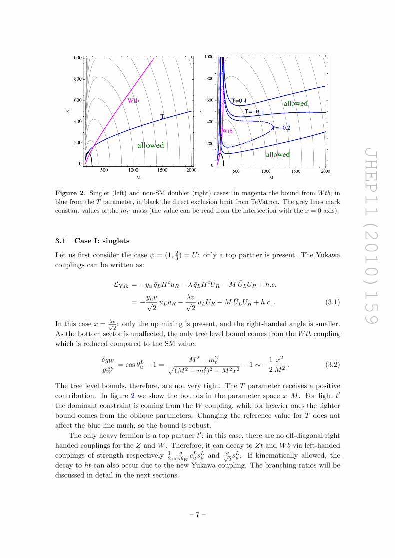
Figure 2. Singlet (left) and non-SM doublet (right) cases: in magenta the bound from Wtb, inblue from the T parameter, in black the direct exclusion limit from TeVatron. The grey lines markconstant values of the mt′ mass (the value can be read from the intersection with the x = 0 axis).
3.1 Case I: singlets
Let us first consider the case ψ = (1, 23) = U : only a top partner is present. The Yukawa
couplings can be written as:
LYuk = −yu qLHcuR − λ qLHcUR −M ULUR + h.c.
= −yuv√2uLuR −
λv√2uLUR −M ULUR + h.c. . (3.1)
In this case x = λv√2: only the up mixing is present, and the right-handed angle is smaller.
As the bottom sector is unaffected, the only tree level bound comes from the Wtb couplingwhich is reduced compared to the SM value:
δgWgsmW
= cos θLu − 1 =M2 −m2
t√(M2 −m2
t )2 +M2x2− 1 ∼ −1
2x2
M2. (3.2)
The tree level bounds, therefore, are not very tight. The T parameter receives a positivecontribution. In figure 2 we show the bounds in the parameter space x–M . For light t′
the dominant constraint is coming from the W coupling, while for heavier ones the tighterbound comes from the oblique parameters. Changing the reference value for T does notaffect the blue line much, so the bound is robust.
The only heavy fermion is a top partner t′: in this case, there are no off-diagonal righthanded couplings for the Z and W . Therefore, it can decay to Zt and Wb via left-handedcouplings of strength respectively 1
2g
cos θWcLus
Lu and g√
2sLu . If kinematically allowed, the
decay to ht can also occur due to the new Yukawa coupling. The branching ratios will bediscussed in detail in the next sections.
– 7 –
JHEP11(2010)159
allowed
T, x=100
T, x=300
Zbb
500 1000 1500 2000
0
50
100
150
200
250
300
M
x_b
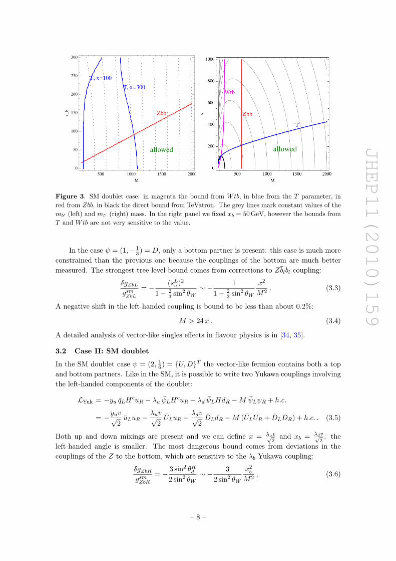
Figure 3. SM doublet case: in magenta the bound from Wtb, in blue from the T parameter, inred from Zbb, in black the direct bound from TeVatron. The grey lines mark constant values of themb′ (left) and mt′ (right) mass. In the right panel we fixed xb = 50 GeV, however the bounds fromT and Wtb are not very sensitive to the value.
In the case ψ = (1,−13) = D, only a bottom partner is present: this case is much more
constrained than the previous one because the couplings of the bottom are much bettermeasured. The strongest tree level bound comes from corrections to Zblbl coupling:
δgZbLgsmZbL
= − (sLu )2
1− 23 sin2 θW
∼ − 11− 2
3 sin2 θW
x2
M2. (3.3)
A negative shift in the left-handed coupling is bound to be less than about 0.2%:
M > 24x . (3.4)
A detailed analysis of vector-like singles effects in flavour physics is in [34, 35].
3.2 Case II: SM doublet
In the SM doublet case ψ = (2, 16) = {U,D}T the vector-like fermion contains both a top
and bottom partners. Like in the SM, it is possible to write two Yukawa couplings involvingthe left-handed components of the doublet:
LYuk = −yu qLHcuR − λu ψLHcuR − λd ψLHdR −M ψLψR + h.c.
= −yuv√2uLuR −
λuv√2ULuR −
λdv√2DLdR −M (ULUR + DLDR) + h.c. . (3.5)
Both up and down mixings are present and we can define x = λuv√2
and xb = λdv√2
: theleft-handed angle is smaller. The most dangerous bound comes from deviations in thecouplings of the Z to the bottom, which are sensitive to the λb Yukawa coupling:
δgZbRgsmZbR
= −3 sin2 θRd2 sin2 θW
∼ − 32 sin2 θW
x2b
M2, (3.6)
– 8 –
JHEP11(2010)159
while the left-handed one is unaffected because D has the same coupling as the left-handedSM down quark.
The only tree level bound on x comes from the left-handed Wtb coupling:
δgWL
gsmW= cos θLu cos θLd + sin θLu sin θLd − 1 ∼ −1
2x2m2
t
M4. (3.7)
Due to the extra m2t suppression, the tree level bounds are mild. There is also a new
right-handed coupling to the W :
gWR
gsmW= sin θRu sin θRd ∼
xxbM2
. (3.8)
The T parameter receives a positive contribution and it depends on both x and xb.From figure 3 we can see that the bound on xb is dominated by the Z coupling: forcomparison we show the bounds from T for x = 100 and 300 GeV showing the strongdependence on x. The figure also shows the bounds on x, as a function of M for xb = 50.The bounds from T and the W coupling do not depend much on the precise value of xb,as long as it is small (xb < 150 GeV in our range of interest). On the other hand, thebound from the Z coupling (red line) does not depend on x and it shifts according to thevalue of xb.
The physical spectrum contains a top partner t′ and a bottom partner b′: the bottompartner is typically lighter that the top one, as long as xb is small, as it can be seen infigure 3. Therefore, the allowed decays are b′ → (Z, h)b and b′ →Wt. On the other hand,t′ → (Z, h)t and t′ → Wb, with the additional channel t′ → Wb′ open if mt′ −mb′ > mW
(for large x).
3.3 Case III: non-SM doublets
In the case ψ = (2, 76) = {X,U}T , the vector-like fermion contains a top partner together
with a new fermion X with charge 53 . The Yukawa couplings involve the left-handed
component of ψ:
LYuk = −yu qLHcuR − λ ψLHuR −M ψLψR + h.c.
= −yuv√2uLuR −
λv√2ULuR −M (ULUR + XLXR) + h.c. . (3.9)
In this case x = λv√2: only the up mixing is present, and the left-handed angle is smaller.
The only tree level bound comes from the left-handed Wtb coupling:
δgWgsmW
= cos θLu − 1 ∼ −12x2m2
t
M4. (3.10)
Due to the extra m2t suppression, the tree level bounds are negligible. The T parameter
can receive both a positive and a negative contribution. For positive T we fix the bound at0.4, and the curve does not depend much on the precise value (solid blue line in figure 2).For negative contributions, we impose a tighter bound at −0.2, the reason being that it is
– 9 –
JHEP11(2010)159
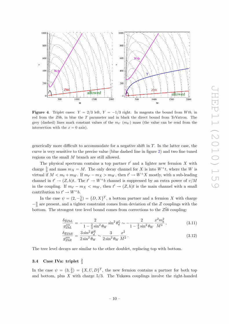
Figure 4. Triplet cases: Y = 2/3 left, Y = −1/3 right. In magenta the bound from Wtb, inred from the Zbb, in blue the T parameter and in black the direct bound from TeVatron. Thegrey (dashed) lines mark constant values of the mt′ (mb′) mass (the value can be read from theintersection with the x = 0 axis).
generically more difficult to accommodate for a negative shift in T . In the latter case, thecurve is very sensitive to the precise value (blue dashed line in figure 2) and two fine tunedregions on the small M branch are still allowed.
The physical spectrum contains a top partner t′ and a lighter new fermion X withcharge 5
3 and mass mX = M . The only decay channel for X is into W+t, where the W isvirtual if M < mt +mW . If mt′ −mX > mW , then t′ →W+X mostly, with a sub-leadingchannel in t′ → (Z, h)t. The t′ → W+b channel is suppressed by an extra power of v/Min the coupling. If mt′ −mX < mW , then t′ → (Z, h)t is the main channel with a smallcontribution to t′ →W+b.
In the case ψ = (2,−56) = {D,X}T , a bottom partner and a fermion X with charge
−43 are present, and a tighter constraint comes from deviation of the Z couplings with the
bottom. The strongest tree level bound comes from corrections to the Zbb coupling:
δgZbLgsmZbL
= − 21− 2
3 sin2 θWsin2 θLd ∼ −
21− 2
3 sin2 θW
x2m2b
M4, (3.11)
δgZbRgsmZbR
=3 sin2 θRd2 sin2 θW
∼ 32 sin2 θW
x2
M2. (3.12)
The tree level decays are similar to the other doublet, replacing top with bottom.
3.4 Case IVa: triplet 23
In the case ψ = (3, 23) = {X,U,D}T , the new fermion contains a partner for both top
and bottom, plus X with charge 5/3. The Yukawa couplings involve the right-handed
– 10 –
JHEP11(2010)159
component of ψ:
LYuk = −yu qLHcuR − λ qLτaHcψaR −M ψLψR + h.c. (3.13)
= −yuv√2uLuR −
λv√2uLUR − λv dLDR −M (ULUR + DLDR + XLXR) + h.c. .
The new Yukawa, therefore, induces a mixing both in the top and bottom sector: definingas usual x = λv√
2, for the top the same formulas as in case I apply, while for the bottom it
suffices to replace x→√
2x. From figure 4 we can see that in most of the parameter space,especially on the large M branch, mb′ > mt′ > mX .
The presence of a bottom partner induces deviations in the couplings to the Z:
δgZbLgsmZbL
=1
1− 23 sin2 θW
sin2 θLd ∼2
1− 23 sin2 θW
x2
M2, (3.14)
δgZbRgsmZbR
= −3 sin2 θRdsin2 θW
∼ − 6sin2 θW
x2m2b
M4. (3.15)
The strongest bound is therefore coming from the positive deviation to the left-handedcoupling. We also computed the T parameter, however it is small and does not pose anyfurther bound. From figure 4 we can see that the Z coupling bound is very tight indeedand the new Yukawa x has to be smaller than about 100 GeV in the range of masseswe considered.
The spectrum contains tree new particles, X, t′ and b′: the lightest one is always theX (mX = M) which decays in W+t (with a virtual W for very light M). For the heavytop, t′ → (Z, h)t and t′ →Wb are the main modes together with t′ →WX. For the heavybottom, b′ → (Z, h)b and b′ →Wt are the main modes together with b′ →Wt′.
3.5 Case IVb: triplet −13
In the case ψ = (3,−13) = {U,D,X}T , the new fermion contains a partner for both top
and bottom, plus X with charge −4/3. The Yukawa couplings involve the right-handedcomponent of ψ:
LYuk = −yu qLHcuR − λ qLτaHψaR −M ψLψR + h.c. (3.16)
= −yuv√2uLuR − λv uLUR +
λv√2dLDR −M (ULUR + DLDR + XLXR) + h.c. .
As before, the new Yukawa induces a mixing both in the top and bottom sector: definingas usual x = λv√
2, for the top the same formulas as in case I apply with x →
√2x, while
for the bottom it suffices to replace x → −x. From figure 4 we can see that in the wholeparameter space mt′ > mb′ > mX .
The presence of a bottom partner induces deviations in the left-handed couplingto the Z:
δgZbLgsmZbL
= − 11− 2
3 sin2 θWsin2 θLd ∼ −
11− 2
3 sin2 θW
x2
M2. (3.17)
– 11 –
JHEP11(2010)159
The strongest bound is therefore coming from the negative deviation to the left-handedcoupling. The T parameter receives a positive contribution, however as it can be seen fromfigure 4 the bound is always weaker than the tree level one. Like in the previous case, thenew Yukawa x has to be smaller than about 100 GeV in the range of masses we considered.
The spectrum contains tree new particles, X, t′ and b′: the lightest one is always theX which decays in W−b. For the heavy bottom, b′ → (Z, h)b and b′ → Wt are the mainmodes together with b′ → WX. For the heavy bottom, t′ → (Z, h)t and t′ → Wb are themain modes together with t′ →Wb′.
4 Tree level and radiative decays
The main decay modes of the heavy fermions is via heavy gauge bosons, the W and Z, andthe Higgs boson h. The width is effectively controlled by the new Yukawa coupling λ, whichgenerates the mixing with the light fermions. Generically, all those modes are present butthe relative ratios depend crucially on the quantum numbers of the new fermion. Thesemodes are also crucial for the observation of the new states at the LHC [36, 37]. At looplevel, new channels are added, namely decays via emission of a photon or gluon. Eventhough the branching ratio is suppressed by a loop, the cleanness of the photon modemay be important for LHC strategies. Moreover, those loops may be enhanced in the caseof large Yukawa λ and provide a tool to measure it (note that tree level branchings areroughly independent on the size of the Yukawa). Finally, in the case of strong coupling,if the heavy states originate from a strongly interacting sector, those modes may becomecomparable to the tree level decays, and a measurement the modes may give a hint of thecomposite nature of the heavy states.
Pushed by those motivations, we explore here the loop induced decays and calculatethe branching ratios in the perturbative regime, i.e. for small Yukawa λ. Numerically,we consider the one-loop result reliable for x ≤ 500 GeV. A generic matrix element thatdescribes the decay of a heavy fermion F to a light one f plus a vector can be parametrisedas [38, 39]:
M(F → fV ) = f(q1) [(a1pµ + a2q
µ2 + a3γ
µ)L+ (b1pµ + b2qµ2 + b3γ
µ)R]F (q2)εµ(p) , (4.1)
where εµ is the polarisation of the vector and pµ = qµ2 − qµ1 is its momentum, and L and
R are the chirality projectors. This result is valid for general decays into a gauge boson(massive or not). In the case of a massless one, therefore unbroken gauge symmetry, theconservation of the fermionic current (M(εµ = pµ) = 0) implies that:
a3 = −12
(mfa2 +mF b2) , (4.2)
b3 = −12
(mFa2 +mfb2) , (4.3)
when the external boson is on-shell, p2 = 0. Here, mF and mf are the masses of the heavyand light fermions. The partial width can be expressed in terms of those parameters:
Γ(F → fγ) =λ1/2(1, 0,m2
f/m2F ) mF
64π
(1−
m2f
m2F
)2 (|mFa2|2 + |mF b2|2
); (4.4)
– 12 –
JHEP11(2010)159
where the phase space function λ1/2(x1, x2, x3) =√x2
1 + x22 + x2
3 − 2x1x2 − 2x1x3 − 2x2x3.For the gluon, an extra colour factor of 4/3 must be added; for a massive boson, a moregeneral formula applies that can be found in [38, 39]. The general one loop contributionsto the matrix element in eq. (4.1) are listed in appendix A.
The general formula can be also used to calculate the tree level decay widths intoheavy gauge bosons: in this case, the left- and right-handed couplings are given by a3 andb3 while all the other parameters vanish. The width is given by:
Γ(F → f ′V ) =λ1/2(1,m2
V /m2F ,m
2f/m
2F )m3
F
32πm2V
(|a3|2 + |b3|2
)·(1−
m2f
m2F
)2
−2m4V
m4F
+m2V
m2F
+ |!m2fm
2V
m4F
−12mfm
2V
m3F
Rea3Re b3+Ima3 Im b3|a3|2 + |b3|2
(4.5)
where Re and Im indicate respectively the real and imaginary part. The tree level widthsfor all the cases are explicitly given in appendix B.2.
5 Numerical results
In this section we report numerical results for the tree and one-loop level branching ratiosin the various cases. As a reference, we fix mh = 120 GeV, and we limit the plots tomt′ < 1 TeV. For larger masses, the production cross section at the LHC is too small tolead to a clear signature (see figure 9). In all cases we will plot curves corresponding tovarious values of x as a function of the t′ mass. The point is to show the possible rangeof values for the branching ratios (BR) as a function of the mass. The relative importanceof the tree level decays is typically controlled by the representation of the new fermion,therefore observing those modes can help to discriminate between the different cases. Inall the plots, the continuous line corresponds to parameter space that is allowed by allconstraints, while the dotted part of the lines are excluded by the T parameter only andtherefore may be allowed if new contributions are present. All the numerical results arebased on the formulas provided in appendix A and B.2.
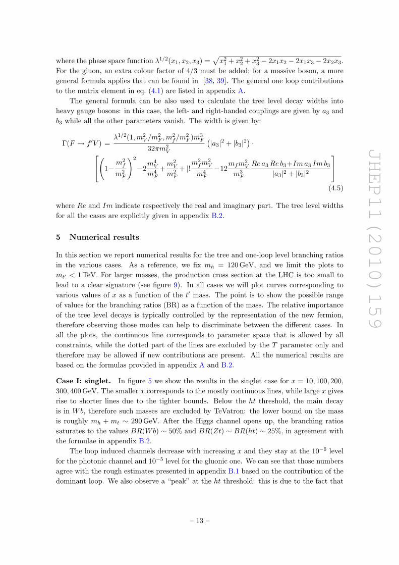
Case I: singlet. In figure 5 we show the results in the singlet case for x = 10, 100, 200,300, 400 GeV. The smaller x corresponds to the mostly continuous lines, while large x givesrise to shorter lines due to the tighter bounds. Below the ht threshold, the main decayis in Wb, therefore such masses are excluded by TeVatron: the lower bound on the massis roughly mh + mt ∼ 290 GeV. After the Higgs channel opens up, the branching ratiossaturates to the values BR(Wb) ∼ 50% and BR(Zt) ∼ BR(ht) ∼ 25%, in agreement withthe formulae in appendix B.2.
The loop induced channels decrease with increasing x and they stay at the 10−6 levelfor the photonic channel and 10−5 level for the gluonic one. We can see that those numbersagree with the rough estimates presented in appendix B.1 based on the contribution of thedominant loop. We also observe a “peak” at the ht threshold: this is due to the fact that
– 13 –
JHEP11(2010)159
W b
Z t
200 400 600 800 10000.0
0.2
0.4
0.6
0.8
1.0
mt'
BR
h t
200 400 600 800 10000.0
0.2
0.4
0.6
0.8
1.0
mt'
BR
Γ t
200 400 600 800 10000.0
0.1
0.2
0.3
0.4
0.5
mt'
105
�B
R
g t
200 400 600 800 10000
1
2
3
4
5
6
mt'
105
�B
R
Figure 5. Singlet case: the lines correspond to x = 10, 100, 200, 300, 400 GeV from darker (blue) tolighter gray (green); the dotted portions are excluded by the T parameter. The vertical line marksthe direct exclusion by TeVatron, which roughly corresponds to 290 GeV.
below such threshold the total width decreases sharply, while the loop one increases. Afterthe threshold, the contribution of the Higgs channel increases the total width, thus pushingdown the BR. Above threshold, we also observe a point where the BR starts decreasingdue to a decrease in the partial width.
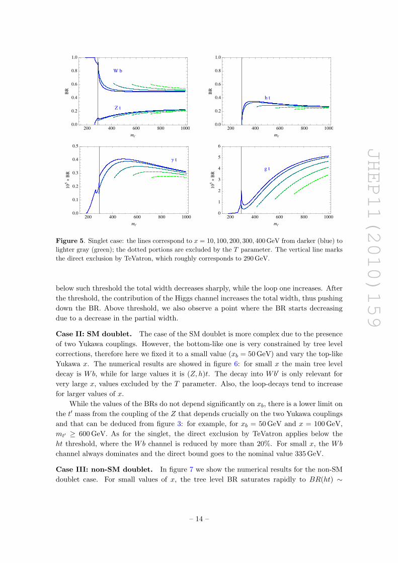
Case II: SM doublet. The case of the SM doublet is more complex due to the presenceof two Yukawa couplings. However, the bottom-like one is very constrained by tree levelcorrections, therefore here we fixed it to a small value (xb = 50 GeV) and vary the top-likeYukawa x. The numerical results are showed in figure 6: for small x the main tree leveldecay is Wb, while for large values it is (Z, h)t. The decay into Wb′ is only relevant forvery large x, values excluded by the T parameter. Also, the loop-decays tend to increasefor larger values of x.
While the values of the BRs do not depend significantly on xb, there is a lower limit onthe t′ mass from the coupling of the Z that depends crucially on the two Yukawa couplingsand that can be deduced from figure 3: for example, for xb = 50 GeV and x = 100 GeV,mt′ ≥ 600 GeV. As for the singlet, the direct exclusion by TeVatron applies below theht threshold, where the Wb channel is reduced by more than 20%. For small x, the Wb
channel always dominates and the direct bound goes to the nominal value 335 GeV.
Case III: non-SM doublet. In figure 7 we show the numerical results for the non-SMdoublet case. For small values of x, the tree level BR saturates rapidly to BR(ht) ∼
– 14 –
JHEP11(2010)159
W b
200 400 600 800 10000.0
0.2
0.4
0.6
0.8
1.0
mt'
BR
Z t
200 400 600 800 10000.0
0.2
0.4
0.6
0.8
1.0
mt''
BR
h t
200 400 600 800 10000.0
0.2
0.4
0.6
0.8
1.0
mt''
BR
W b'
200 400 600 800 10000.0
0.2
0.4
0.6
0.8
1.0
mt''
BR
Γ t
200 400 600 800 10000.0
0.1
0.2
0.3
0.4
0.5
0.6
mt''
105
�B
R
g t
200 400 600 800 10000
1
2
3
4
5
mt''
105
�B
R
Figure 6. SM doublet: the lines correspond to xb = 50 GeV and x =10, 25, 50, 75, 100, 200, 300, 400, 500 GeV from darker (blue) to lighter grey (green). The dottedlines are excluded by the T parameter. The vertical line marks the direct exclusion by TeVatron.
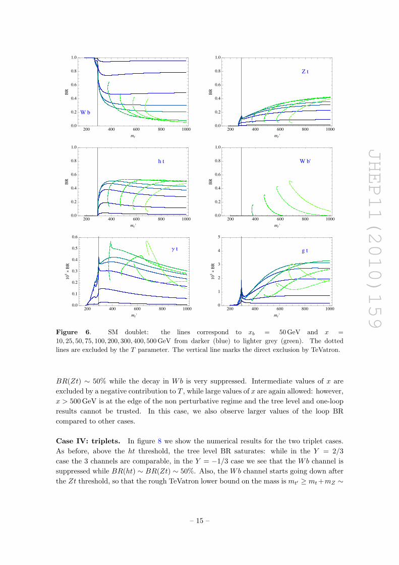
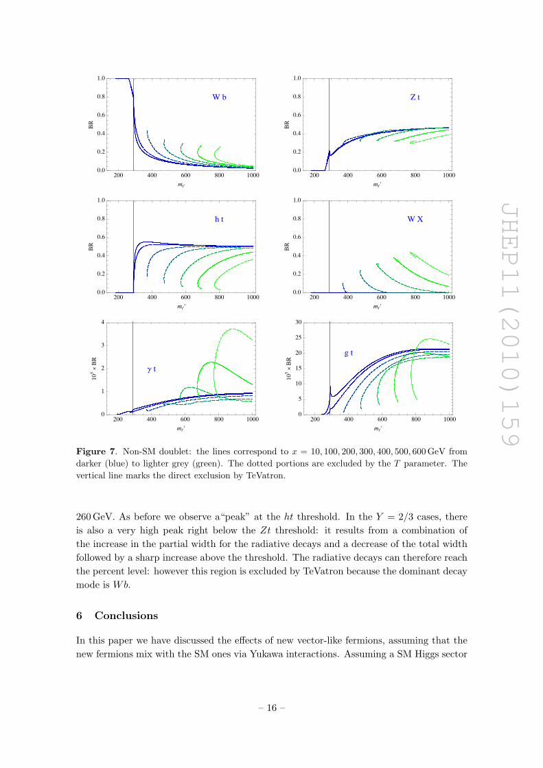
BR(Zt) ∼ 50% while the decay in Wb is very suppressed. Intermediate values of x areexcluded by a negative contribution to T , while large values of x are again allowed: however,x > 500 GeV is at the edge of the non perturbative regime and the tree level and one-loopresults cannot be trusted. In this case, we also observe larger values of the loop BRcompared to other cases.
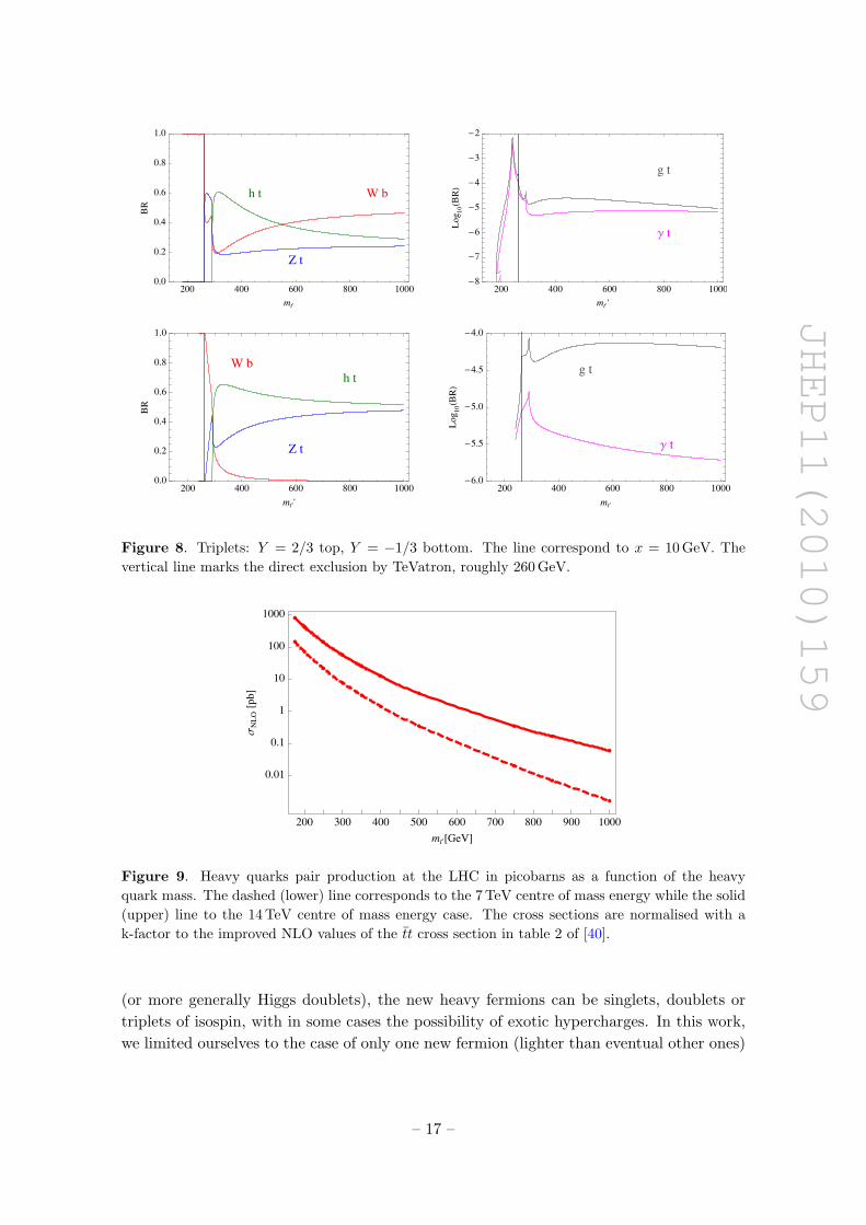
Case IV: triplets. In figure 8 we show the numerical results for the two triplet cases.As before, above the ht threshold, the tree level BR saturates: while in the Y = 2/3case the 3 channels are comparable, in the Y = −1/3 case we see that the Wb channel issuppressed while BR(ht) ∼ BR(Zt) ∼ 50%. Also, the Wb channel starts going down afterthe Zt threshold, so that the rough TeVatron lower bound on the mass is mt′ ≥ mt+mZ ∼
– 15 –
JHEP11(2010)159
W b
200 400 600 800 10000.0
0.2
0.4
0.6
0.8
1.0
mt'
BR
Z t
200 400 600 800 10000.0
0.2
0.4
0.6
0.8
1.0
mt''
BR
h t
200 400 600 800 10000.0
0.2
0.4
0.6
0.8
1.0
mt''
BR
W X
200 400 600 800 10000.0
0.2
0.4
0.6
0.8
1.0
mt''
BR
Γ t
200 400 600 800 10000
1
2
3
4
mt''
105
�B
R
g t
200 400 600 800 10000
5
10
15
20
25
30
mt''
105
�B
R
Figure 7. Non-SM doublet: the lines correspond to x = 10, 100, 200, 300, 400, 500, 600 GeV fromdarker (blue) to lighter grey (green). The dotted portions are excluded by the T parameter. Thevertical line marks the direct exclusion by TeVatron.
260 GeV. As before we observe a“peak” at the ht threshold. In the Y = 2/3 cases, thereis also a very high peak right below the Zt threshold: it results from a combination ofthe increase in the partial width for the radiative decays and a decrease of the total widthfollowed by a sharp increase above the threshold. The radiative decays can therefore reachthe percent level: however this region is excluded by TeVatron because the dominant decaymode is Wb.
6 Conclusions
In this paper we have discussed the effects of new vector-like fermions, assuming that thenew fermions mix with the SM ones via Yukawa interactions. Assuming a SM Higgs sector
– 16 –
JHEP11(2010)159
W b
Z t
h t
200 400 600 800 10000.0
0.2
0.4
0.6
0.8
1.0
mt'
BR
Γ t
g t
200 400 600 800 1000-8
-7
-6
-5
-4
-3
-2
mt''
Log
10HB
RL
W b
Z t
h t
200 400 600 800 10000.0
0.2
0.4
0.6
0.8
1.0
mt''
BR
Γ t
g t
200 400 600 800 1000-6.0
-5.5
-5.0
-4.5
-4.0
mt'
Log
10HB
RL
Figure 8. Triplets: Y = 2/3 top, Y = −1/3 bottom. The line correspond to x = 10 GeV. Thevertical line marks the direct exclusion by TeVatron, roughly 260 GeV.
200 300 400 500 600 700 800 900 1000
0.01
0.1
1
10
100
1000
mt'@GeVD
Σ
NL
O@pb
D
Figure 9. Heavy quarks pair production at the LHC in picobarns as a function of the heavyquark mass. The dashed (lower) line corresponds to the 7 TeV centre of mass energy while the solid(upper) line to the 14 TeV centre of mass energy case. The cross sections are normalised with ak-factor to the improved NLO values of the tt cross section in table 2 of [40].
(or more generally Higgs doublets), the new heavy fermions can be singlets, doublets ortriplets of isospin, with in some cases the possibility of exotic hypercharges. In this work,we limited ourselves to the case of only one new fermion (lighter than eventual other ones)
– 17 –
JHEP11(2010)159
case Wb Zt ht γt gt
Singlet, x = 10 0.50 0.17 0.33 4 ×10⁻⁶ 2.7 ×10⁻⁵
Singlet, x = 200 0.50 0.15 0.29 3 ×10⁻⁶ 1.6 ×10⁻⁵
SM doublet, x = 10 0.95 0.017 0.03 0.21 ×10⁻⁶ 0.2 ×10⁻⁵
SM doublet, x = 100 0.24 0.26 0.50 4 ×10⁻⁶ 2.2 ×10⁻⁵
Non-SM doublet, x = 10 0.09 0.37 0.61 6 ×10⁻⁶ 15 ×10−5
Triplet A (Y=2/3), x = 10 0.36 0.22 0.42 7.2 ×10⁻⁶ 2.4 ×10⁻⁵
Triplet B (Y=-1/3), x = 10 0.01 0.41 0.58 3.5 ×10⁻⁶ 7.1 ×10⁻⁵
Table 1. Typical values for the branching ratios in the various cases, for mt′ = 500 GeV.
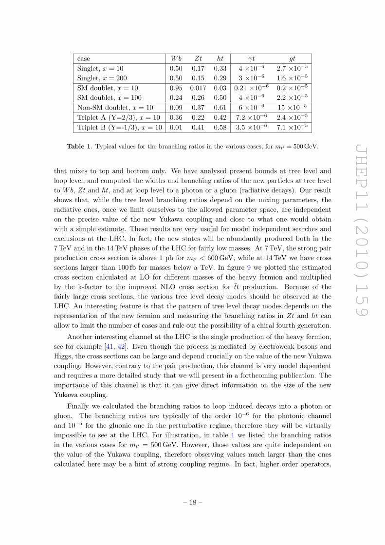
that mixes to top and bottom only. We have analysed present bounds at tree level andloop level, and computed the widths and branching ratios of the new particles at tree levelto Wb, Zt and ht, and at loop level to a photon or a gluon (radiative decays). Our resultshows that, while the tree level branching ratios depend on the mixing parameters, theradiative ones, once we limit ourselves to the allowed parameter space, are independenton the precise value of the new Yukawa coupling and close to what one would obtainwith a simple estimate. These results are very useful for model independent searches andexclusions at the LHC. In fact, the new states will be abundantly produced both in the7 TeV and in the 14 TeV phases of the LHC for fairly low masses. At 7 TeV, the strong pairproduction cross section is above 1 pb for mt′ < 600 GeV, while at 14 TeV we have crosssections larger than 100 fb for masses below a TeV. In figure 9 we plotted the estimatedcross section calculated at LO for different masses of the heavy fermion and multipliedby the k-factor to the improved NLO cross section for tt production. Because of thefairly large cross sections, the various tree level decay modes should be observed at theLHC. An interesting feature is that the pattern of tree level decay modes depends on therepresentation of the new fermion and measuring the branching ratios in Zt and ht canallow to limit the number of cases and rule out the possibility of a chiral fourth generation.
Another interesting channel at the LHC is the single production of the heavy fermion,see for example [41, 42]. Even though the process is mediated by electroweak bosons andHiggs, the cross sections can be large and depend crucially on the value of the new Yukawacoupling. However, contrary to the pair production, this channel is very model dependentand requires a more detailed study that we will present in a forthcoming publication. Theimportance of this channel is that it can give direct information on the size of the newYukawa coupling.
Finally we calculated the branching ratios to loop induced decays into a photon orgluon. The branching ratios are typically of the order 10−6 for the photonic channeland 10−5 for the gluonic one in the perturbative regime, therefore they will be virtuallyimpossible to see at the LHC. For illustration, in table 1 we listed the branching ratiosin the various cases for mt′ = 500 GeV. However, those values are quite independent onthe value of the Yukawa coupling, therefore observing values much larger than the onescalculated here may be a hint of strong coupling regime. In fact, higher order operators,
– 18 –
JHEP11(2010)159
generated by the strong coupling, do contribute equally to the W , Z and γ channels: ifthose operators are large, we would expect order one branching ratios in photon, as typicalof an excited fermion. Larger values of the loop induced channels may also be generatedby heavier states running in the loop and not directly observed at the LHC. In this case,the loop may be enhanced by large couplings in the heavy sector. Nevertheless, in theperturbative regime, such new contribution would be loop suppressed and therefore cannot enhance the channel by orders of magnitude. In this sense, we conclude that underour assumptions that only one “light” vector-like fermion is present, the observation ofthe γt or gt channels at the LHC hints to a strong coupling dynamic as the origin of thenew state.
Acknowledgments
The research of Y.O. is supported in part by the Grant-in-Aid for Science Research, Min-istry of Education, Culture, Sports, Science and Technology (MEXT), Japan, No. 16081211and by the Grant-in-Aid for Science Research, Japan Society for the Promotion of Science(JSPS), No. 20244037 and No. 22244031. This collaboration was made possible by fund-ing by the French “Ministere des Affaires Etrangeres” and the Japanese JSPS under aPHC-SAKURA project No. 18763QK.
A General loop calculation formulas
We will assume that the vector V in the loop, with mass MV , has both left- and right-handed couplings with a generic pair of fermions:
f γµVµ (gLff ′L+ gRff ′R) f ′ ; (A.1)
while a scalar boson φ has couplings:
f (λLff ′L+ λRff ′R)φ f ′ . (A.2)
In our calculation, we use ’t Hooft-Feynman gauge and take the external quarks t′, t to beon shell. The t′ → tγ(tg) transition matrix element is given by
M = t(q1)Γµrent′(q2)εµ(λ), (A.3)
where Γµren is renormalised electromagnetic (strong) current and εµ is the polarisation vectorof the gauge boson. In this case, the form factor of electromagnetic current is given by
Γµren = Γµ + TLγµL+ TRγ
µR. (A.4)
The unrenormalised current Γµ can be written in the following form
Γµ = (a1pµ + a2q
µ2 + a3γ
µ)L+ (b1pµ + b2qµ2 + b3γ
µ)R, (A.5)
where the form factors ai and bi are sums of the contributions from all diagrams in theprocess. We perform our loop calculations in D dimensions and define ε = 4 − D. In
– 19 –
JHEP11(2010)159
k + p
t
0
t
p
( g )
tt
0
( g )
t
0
( g )
t
( d )
( a ) ( b )
( g )
( e )
tt
0
( g )
( c )
( g ) ( g )
( j )
t
0
t
0
t
t
t
0
t
0
t t
ttt
0
t
0
( h ) ( i )
( f )
k � q
1
k � q
2
q
1
k � q
1
q
2
k k
k
k + q
1
k
p � k
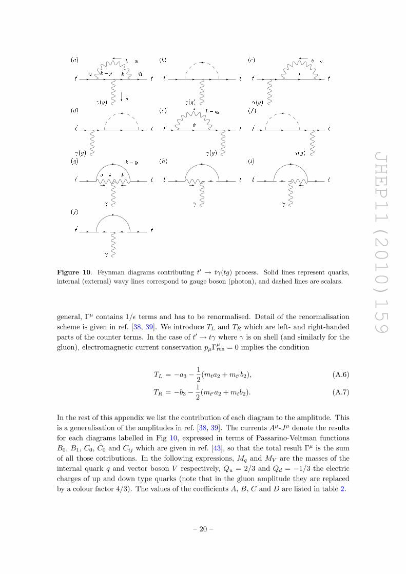
Figure 10. Feynman diagrams contributing t′ → tγ(tg) process. Solid lines represent quarks,internal (external) wavy lines correspond to gauge boson (photon), and dashed lines are scalars.
general, Γµ contains 1/ε terms and has to be renormalised. Detail of the renormalisationscheme is given in ref. [38, 39]. We introduce TL and TR which are left- and right-handedparts of the counter terms. In the case of t′ → tγ where γ is on shell (and similarly for thegluon), electromagnetic current conservation pµΓµren = 0 implies the condition
TL = −a3 −12
(mta2 +mt′b2), (A.6)
TR = −b3 −12
(mt′a2 +mtb2). (A.7)
In the rest of this appendix we list the contribution of each diagram to the amplitude. Thisis a generalisation of the amplitudes in ref. [38, 39]. The currents Aµ-Jµ denote the resultsfor each diagrams labelled in Fig 10, expressed in terms of Passarino-Veltman functionsB0, B1, C0, C0 and Cij which are given in ref. [43], so that the total result Γµ is the sumof all those cotributions. In the following expressions, Mq and MV are the masses of theinternal quark q and vector boson V respectively, Qu = 2/3 and Qd = −1/3 the electriccharges of up and down type quarks (note that in the gluon amplitude they are replacedby a colour factor 4/3). The values of the coefficients A, B, C and D are listed in table 2.
– 20 –
JHEP11(2010)159
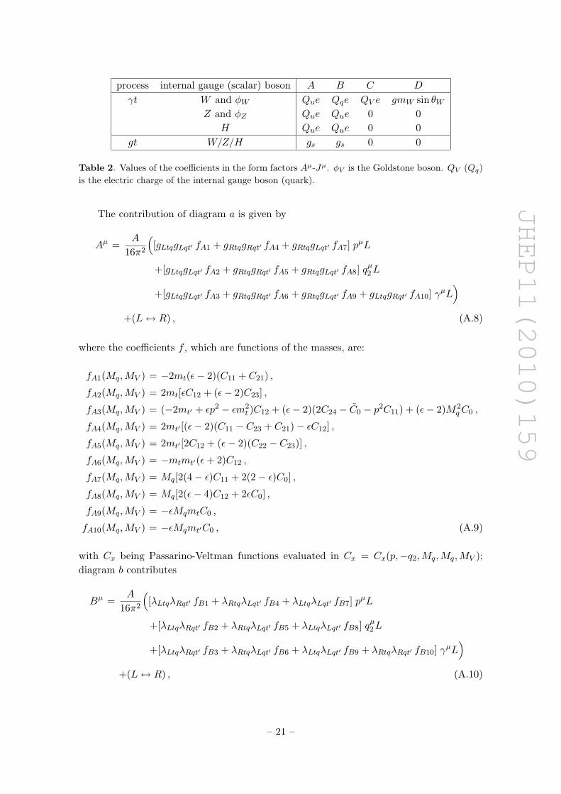
process internal gauge (scalar) boson A B C D
γt W and φW Que Qqe QV e gmW sin θWZ and φZ Que Que 0 0
H Que Que 0 0gt W/Z/H gs gs 0 0
Table 2. Values of the coefficients in the form factors Aµ-Jµ. φV is the Goldstone boson. QV (Qq)is the electric charge of the internal gauge boson (quark).
The contribution of diagram a is given by
Aµ =A
16π2
([gLtqgLqt′ fA1 + gRtqgRqt′ fA4 + gRtqgLqt′ fA7] pµL
+[gLtqgLqt′ fA2 + gRtqgRqt′ fA5 + gRtqgLqt′ fA8] qµ2L
+[gLtqgLqt′ fA3 + gRtqgRqt′ fA6 + gRtqgLqt′ fA9 + gLtqgRqt′ fA10] γµL)
+(L↔ R) , (A.8)
where the coefficients f , which are functions of the masses, are:
fA1(Mq,MV ) = −2mt(ε− 2)(C11 + C21) ,
fA2(Mq,MV ) = 2mt[εC12 + (ε− 2)C23] ,
fA3(Mq,MV ) = (−2mt′ + εp2 − εm2t )C12 + (ε− 2)(2C24 − C0 − p2C11) + (ε− 2)M2
qC0 ,
fA4(Mq,MV ) = 2mt′ [(ε− 2)(C11 − C23 + C21)− εC12] ,
fA5(Mq,MV ) = 2mt′ [2C12 + (ε− 2)(C22 − C23)] ,
fA6(Mq,MV ) = −mtmt′(ε+ 2)C12 ,
fA7(Mq,MV ) = Mq[2(4− ε)C11 + 2(2− ε)C0] ,
fA8(Mq,MV ) = Mq[2(ε− 4)C12 + 2εC0] ,
fA9(Mq,MV ) = −εMqmtC0 ,
fA10(Mq,MV ) = −εMqmt′C0 , (A.9)
with Cx being Passarino-Veltman functions evaluated in Cx = Cx(p,−q2,Mq,Mq,MV );diagram b contributes
Bµ =A
16π2
([λLtqλRqt′ fB1 + λRtqλLqt′ fB4 + λLtqλLqt′ fB7] pµL
+[λLtqλRqt′ fB2 + λRtqλLqt′ fB5 + λLtqλLqt′ fB8] qµ2L
+[λLtqλRqt′ fB3 + λRtqλLqt′ fB6 + λLtqλLqt′ fB9 + λRtqλRqt′ fB10] γµL)
+(L↔ R) , (A.10)
– 21 –
JHEP11(2010)159
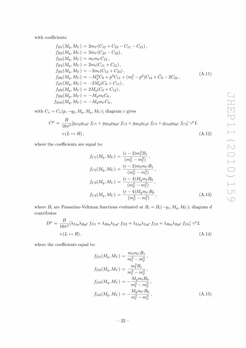
with coefficients:
fB1(Mq,MV ) = 2mt′(C12 + C23 − C11 − C21) ,fB2(Mq,MV ) = 2mt′(C23 − C22) ,fB3(Mq,MV ) = mtmt′C12 ,
fB4(Mq,MV ) = 2mt(C11 + C21) ,fB5(Mq,MV ) = −2mt(C12 + C23) ,fB6(Mq,MV ) = −M2
qC0 + p2C11 + (m2t − p2)C12 + C0 − 2C24 ,
fB7(Mq,MV ) = −2Mq(C0 + C11) ,fB8(Mq,MV ) = 2Mq(C0 + C12) ,fB9(Mq,MV ) = −MqmtC0 ,
fB10(Mq,MV ) = −Mqmt′C0 ,
(A.11)
with Cx = Cx(p,−q2,Mq,Mq,MV ); diagram c gives
Cµ =B
16π2[gLtqgLqt′ fC1 + gRtqgRqt′ fC2 + gRtqgLqt′ fC3 + gLtqgRqt′ fC4] γµL
+(L↔ R) , (A.12)
where the coefficients are equal to:
fC1(Mq,MV ) =(ε− 2)m2
tB1
(m2t′ −m2
t ),
fC2(Mq,MV ) =(ε− 2)mtmt′B1
(m2t′ −m2
t ),
fC3(Mq,MV ) =(ε− 4)MqmtB0
(m2t′ −m2
t ),
fC4(Mq,MV ) =(ε− 4)Mqmt′B0
(m2t′ −m2
t ), (A.13)
where Bi are Passarino-Veltman functions evaluated at Bi = Bi(−q1,Mq,MV ); diagram d
contributes
Dµ =B
16π2[λLtqλRqt′ fD1 + λRtqλLqt′ fD2 + λLtqλLqt′ fD3 + λRtqλRqt′ fD4] γµL
+(L↔ R) , (A.14)
where the coefficients equal to:
fD1(Mq,MV ) =mtmt′B1
m2t −m2
t′,
fD2(Mq,MV ) =m2tB1
m2t −m2
t′,
fD3(Mq,MV ) = −MqmtB0
m2t −m2
t′,
fD4(Mq,MV ) = −Mqmt′B0
m2t −m2
t′, (A.15)
– 22 –
JHEP11(2010)159
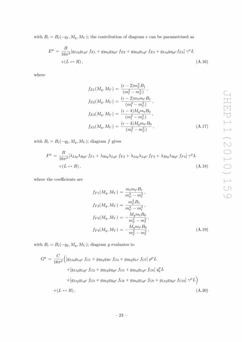
with Bi = Bi(−q1,Mq,MV ); the contribution of diagram e can be parametrised as
Eµ =B
16π2[gLtqgLqt′ fE1 + gRtqgRqt′ fE2 + gRtqgLqt′ fE3 + gLtqgRqt′fE4] γµL
+(L↔ R) , (A.16)
where
fE1(Mq,MV ) =(ε− 2)m2
t′B1
(m2t −m2
t′),
fE2(Mq,MV ) =(ε− 2)mtmt′B1
(m2t −m2
t′),
fE3(Mq,MV ) =(ε− 4)MqmtB0
(m2t −m2
t′),
fE4(Mq,MV ) =(ε− 4)Mqmt′B0
(m2t −m2
t′), (A.17)
with Bi = Bi(−q2,Mq,MV ); diagram f gives
Fµ =B
16π2[λLtqλRqt′ fF1 + λRtqλLqt′ fF2 + λLtqλLqt′ fF3 + λRtqλRqt′ fF4] γµL
+(L↔ R) , (A.18)
where the coefficients are
fF1(Mq,MV ) =mtmt′B1
m2t′ −m2
t
,
fF2(Mq,MV ) =m2t′B1
m2t′ −m2
t
,
fF3(Mq,MV ) = −MqmtB0
m2t′ −m2
t
,
fF4(Mq,MV ) = −Mqmt′B0
m2t′ −m2
t
, (A.19)
with Bi = Bi(−q2,Mq,MV ); diagram g evaluates to
Gµ =C
16π2
([gLtqgLqt′ fG1 + gRtqgRt′ fG4 + gRtqgLt′ fG7] pµL
+[gLtqgLqt′ fG2 + gRtqgRqt′ fG5 + gRtqgLqt′ fG8] qµ2L
+[gLtqgLqt′ fG3 + gRtqgRqt′ fG6 + gRtqgLqt′ fG9 + gLtqgRqt′ fG10] γµL)
+(L↔ R) , (A.20)
– 23 –
JHEP11(2010)159
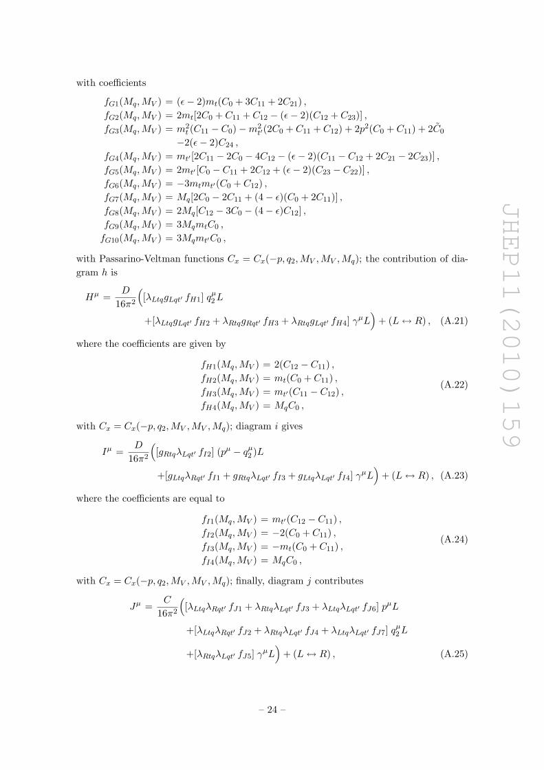
with coefficients
fG1(Mq,MV ) = (ε− 2)mt(C0 + 3C11 + 2C21) ,fG2(Mq,MV ) = 2mt[2C0 + C11 + C12 − (ε− 2)(C12 + C23)] ,fG3(Mq,MV ) = m2
t (C11 − C0)−m2t′(2C0 + C11 + C12) + 2p2(C0 + C11) + 2C0
−2(ε− 2)C24 ,
fG4(Mq,MV ) = mt′ [2C11 − 2C0 − 4C12 − (ε− 2)(C11 − C12 + 2C21 − 2C23)] ,fG5(Mq,MV ) = 2mt′ [C0 − C11 + 2C12 + (ε− 2)(C23 − C22)] ,fG6(Mq,MV ) = −3mtmt′(C0 + C12) ,fG7(Mq,MV ) = Mq[2C0 − 2C11 + (4− ε)(C0 + 2C11)] ,fG8(Mq,MV ) = 2Mq[C12 − 3C0 − (4− ε)C12] ,fG9(Mq,MV ) = 3MqmtC0 ,
fG10(Mq,MV ) = 3Mqmt′C0 ,
with Passarino-Veltman functions Cx = Cx(−p, q2,MV ,MV ,Mq); the contribution of dia-gram h is
Hµ =D
16π2
([λLtqgLqt′ fH1] qµ2L
+[λLtqgLqt′ fH2 + λRtqgRqt′ fH3 + λRtqgLqt′ fH4] γµL)
+ (L↔ R) , (A.21)
where the coefficients are given by
fH1(Mq,MV ) = 2(C12 − C11) ,fH2(Mq,MV ) = mt(C0 + C11) ,fH3(Mq,MV ) = mt′(C11 − C12) ,fH4(Mq,MV ) = MqC0 ,
(A.22)
with Cx = Cx(−p, q2,MV ,MV ,Mq); diagram i gives
Iµ =D
16π2
([gRtqλLqt′ fI2] (pµ − qµ2 )L
+[gLtqλRqt′ fI1 + gRtqλLqt′ fI3 + gLtqλLqt′ fI4] γµL)
+ (L↔ R) , (A.23)
where the coefficients are equal to
fI1(Mq,MV ) = mt′(C12 − C11) ,fI2(Mq,MV ) = −2(C0 + C11) ,fI3(Mq,MV ) = −mt(C0 + C11) ,fI4(Mq,MV ) = MqC0 ,
(A.24)
with Cx = Cx(−p, q2,MV ,MV ,Mq); finally, diagram j contributes
Jµ =C
16π2
([λLtqλRqt′ fJ1 + λRtqλLqt′ fJ3 + λLtqλLqt′ fJ6] pµL
+[λLtqλRqt′ fJ2 + λRtqλLqt′ fJ4 + λLtqλLqt′ fJ7] qµ2L
+[λRtqλLqt′ fJ5] γµL)
+ (L↔ R) , (A.25)
– 24 –
JHEP11(2010)159
with coefficientsfJ1 = mt′(C11 − C12 + 2C21 − 2C23) ,fJ2 = 2mt′(C22 − C23) ,fJ3 = −mt(C0 + 3C11 + 2C21) ,fJ4 = 2mt(C12 + C23) ,fJ5 = 2C24 ,
fJ6 = −Mq(C0 + 2C11) ,fJ7 = 2MqC12 ,
(A.26)
with Cx = Cx(−p, q2,MV ,MV ,Mq).
B Decay width formulas
B.1 A quick estimate
Just to have an idea of the orders of magnitude, we give the tree level widths by computingthe decay of the heavy fermion in W + light fermion (where the dominant channel is inlongitudinal polarisation, i.e. in the Goldstone boson). From eq. 4.5, the width is:
Γ(F →Wf ′) ' λ2mF
32π, (B.1)
where λ is the new Yukawa coupling. This width is equal to the one into Z (long polarisa-tion) and neutral Higgs, therefore if both channels are present the total width is doubled.
For the loop induced one, the graphs directly proportional to the new Yukawa couplingdominate. We will distinguish two cases: Yukawa coupling involving the left-handed F
(case I) and right-handed F (case II). The amplitudes are dominated by the terms:
case I ⇒
mFa2 ' 0
mF b2 'iλλfe
16π2
∑ λqλf
(QqfB1 +QV fJ1)(B.2)
case II ⇒
mFa2 'iλλfe
16π2
∑(QqfB1 +QV fJ1)
mF b2 ' 0(B.3)
Plugging those amplitudes in eq. 4.4, we find:
Γ(F → γf) ' λ2mF
32παewαt32π2
|∑|2 , (B.4)
where we have used the top Yukawa coupling in αt = λ2t /4π, and αem = e2/4π. (Note: for
light fermions f , the top Yukawa may be replaced by the weak α, from diagrams H and I).The branching fraction is therefore:
BR(F → γf) ∼ αewαt32π2
|∑|2 ' 10−6 · |
∑|2 . (B.5)
Note that this is a very conservative estimate, as the sum may contain a log m2F
m2W
enhance-ment which may enhance the result by one or two orders of magnitude.
– 25 –
JHEP11(2010)159
B.2 Decay widths and the the large mass limit
The heavy vector-like fermion t′ can decay at tree level to bW and b′W via a chargedcurrent and to Zt and ht via a neutral current. The t′ → bW and t′ → b′W transitionmatrix elements are given by
M = b(q1)γµ(gWL L+ gWR R)t′(q2)εµ(λ) , (B.6)
where gWL and gWR are left- and right-handed couplings of t′bW (t′b′W ). From eq. 4.5, the
partial width of t′ → bW (b′W ) decay is expressed as
Γ(t′ → bW ) =λ
12
(1, m
2b
m2t′,m2
W
m2t′
)32πmt′
{(|gWL |2 + |gWR |2)
[m2t′ +m2
b − 2m2W +
(m2t′ −m2
b)2
m2W
]
−12(Re gWL Re gWR + ImgWL ImgWR )mt′mb
}(B.7)
where Re and Im indicate respectively the real and imaginary part. In the large mt′ limitthe previous formula becomes
Γ(t′ → b(′)W ) ∼|gWL |2 + |gWR |2
32πm3t′
m2W
(1−
m2b(′)
m2t′
)2
. (B.8)
Concerning neutral currents, the t′ → tZ transition matrix element is written as
M = t(q1)γµ(gZLL+ gZRR)t′(q2)εµ(λ) (B.9)
where gZL and gZR are left- and right-handed couplings of t′tZ. The partial width of t′ →tZ is1
Γ(t′ → tZ) =λ
12
(1, m
2t
m2t′,m2
Z
m2t′
)32πmt′
{(|gZL |2 + |gZR|2)
[m2t′ +m2
t − 2m2Z +
(m2t′ −m2
t )2
m2Z
]
−12(Re gZLRe gZR + ImgZLImgZR)mt′mt
}. (B.10)
In the large t′ mass limit the previous formula can be written in the following form
Γ(t′ → tZ) ∼|gZL |2 + |gZR|2
32πm3t′
m2Z
. (B.11)
For the tree level t′ → th decay, the matrix element is written as
M = t(q1)(CLL+ CRR)t′(q2) (B.12)
1Our expression agrees with the general expression in [28]. It disagrees with the formula given in
hep-ph/0506187, however there is an erratum to this paper (Erratum Phys. Lett. B 633 (2006) 792) which
is consistent with our formula.
– 26 –
JHEP11(2010)159
where CL and CR are left- and right-handed couplings of t′th. The partial width of t′ → th
Γ(t′ → th) =λ
12
(1, m
2t
m2t′,m2
H
m2t′
)32πmt′
{(m2
t′ +m2t −m2
H)(|CL|2 + |CR|2)
+4mt′mt(ReCLReCR + ImCLImCR)}. (B.13)
In the large mt′ limit this becomes
Γ(t′ → th) ∼ |CL|2 + |CR|2
32πmt′ . (B.14)
Singlet case. In the case the new vector-like fermion is a singlet, from the results insection 2.1 we find that the couplings can be written as
gWL =g√2
sin θLu ∼g√2x
M,
gWR = 0 ,
gZL =g
2 cos θWcos θLu sin θLu ∼
g
2 cos θWx
M, (B.15)
gZR = 0 ,
CL = − g
2mWmt cos θLu sin θLu ∼ −
g
2mW
mtx
M,
CR = − g
2mWmt′ cos θLu sin θLu ∼ −
g
2mWx .
In the large mass limit mt′ ∼M � mt, x, the tree level t′ decay widths become
Γ(t′ → bW ) ∼ 132πM
g2
2m2W
x2M2 , (B.16)
Γ(t′ → tZ) ∼ 132πM
g2
4m2Z cos2 θW
x2M2 , (B.17)
Γ(t′ → th) ∼ 132πM
g2
4m2W
x2M2 ; (B.18)
with ratios
Γ(t′ → bW )/Γ(t′ → tZ) =2m2
Z cos2 θWm2W
= 2 , (B.19)
Γ(t′ → th)/Γ(t′ → tZ) =m2Z cos2 θWm2W
= 1 . (B.20)
Therefore, in this limit, the t′ will decay half of the times in Wb, and 25% in Zt and25% in ht.
– 27 –
JHEP11(2010)159
SM doublet case. For a Standard Model like fermion doublet the couplings are given by:
gWL =g√2
sin(θLu − θLd ) ∼ g√2
(mtx
M2− mbxb
M2
),
gWR = − g√2
cos θRu sin θRd ∼ −g√2xbM
,
gZL = 0 , (B.21)
gZR = − g
2 cos θWcos θRu sin θRu ∼ −
g
2 cos θWx
M,
CL = − g
2mWmt′ cos θRu sin θRu ∼ −
g
2mWx ,
CR = − g
2mWmt cos θRu sin θRu ∼ −
g
2mW
mtx
M;
in the large mass limit, the tree level t′ decay widths are
Γ(t′ → bW ) ∼ 132πM
g2
2m2W
x2bM
2 , (B.22)
Γ(t′ → tZ) ∼ 132πM
g2
4m2Z cos2 θW
x2M2 , (B.23)
Γ(t′ → th) ∼ 132πM
g2
4m2W
x2M2 ; (B.24)
with ratios
Γ(t′ → bW )/Γ(t′ → tZ) =2m2
Z cos2 θWm2W
(xbx
)2= 2
(xbx
)2, (B.25)
Γ(t′ → th)/Γ(t′ → tZ) =m2Z cos2 θWm2W
= 1 . (B.26)
For small xb � x, the t′ will always decay in tops and in equal proportions to Z and Higgs.
Non SM doublet case. For a doublet with hypercharge 7/6, the couplings are
gWL =g√2
sin θLu ∼g√2mtx
M2,
gWR = 0 ,
gZL =g
cos θWsin θLu cos θLu ∼
g
cos θWxmt
M2, (B.27)
gZR =g
2 cos θWsin θRu cos θRu ∼
g
2 cos θWx
M,
CL = − g
2mWmt′ cos θRu sin θRu ∼ −
g
2mWx ,
CR = − g
2mWmt cos θRu sin θRu ∼ −
g
2mW
mtx
M;
– 28 –
JHEP11(2010)159
In the large M limit, the tree level t′ decay widths are
Γ(t′ → bW ) ∼ 132πM
g2
2m2W
m2tx
2 , (B.28)
Γ(t′ → tZ) ∼ 132πM
g2
4m2Z cos2 θW
x2M2 , (B.29)
Γ(t′ → th) ∼ 132πM
g2
4m2W
x2M2 ; (B.30)
with ratios
Γ(t′ → bW )/Γ(t′ → tZ) =2m2
Z cos2 θWm2W
m2t
M2= 2
m2t
M2∼ 0 , (B.31)
Γ(t′ → th)/Γ(t′ → tZ) =m2Z cos2 θWm2W
= 1 . (B.32)
The t′ will therefore decay preferably in tops, with equal probability in association of a Zboson or Higgs.
Triplet Y = 2/3 case. For a triplet with hypercharge 2/3:
gWL =g√2
(cos θLd sin θLu −
√2 sin θLd cos θLu
)∼ − g√
2x
M,
gWR =g√2
(−√
2 sin θRd cos θRu)∼ − g√
22xmb
M2,
gZL =g
2 cos θWsin θLu cos θLu ∼
g
2 cos θWx
M, (B.33)
gZR = 0 ,
CL = − g
2mWmt sin θLu cos θLu ∼ −
g
2mW
mtx
M,
CR = − g
2mWmt′ sin θLu cos θLu ∼ −
g
2mWx .
In the large M limit, the tree level t′ decay widths are
Γ(t′ → bW ) ∼ 132πM
g2
2m2W
x2M2 , (B.34)
Γ(t′ → tZ) ∼ 132πM
g2
4m2Z cos2 θW
x2M2 , (B.35)
Γ(t′ → th) ∼ 132πM
g2
4m2W
x2M2 ; (B.36)
with ratios
Γ(t′ → bW )/Γ(t′ → tZ) =2m2
Z cos2 θWm2W
= 2 , (B.37)
Γ(t′ → th)/Γ(t′ → tZ) =m2Z cos2 θWm2W
= 1 . (B.38)
– 29 –
JHEP11(2010)159
Triplet Y = −1/3 case. In the case of a triplet with hypercharge −1/3:
gWL =g√2
(cos θLd sin θLu +
√2 sin θLd cos θLu
)∼ g√
2
√2x3
2M3,
gWR =g√2
(√2 sin θRd cos θRu
)∼ − g√
2
√2xmb
M2,
gZL = − g
2 cos θWsin θLu cos θLu ∼ −
g
2 cos θW
√2xM
, (B.39)
gZR = − g
cos θWcos θRu sin θRu ∼ −
g
cos θW
√2xmt
M2,
CL = − g
2mWmt sin θLu cos θLu ∼ −
g
2mW
√2xmt
M, (B.40)
CR = − g
2mWmt′ sin θLu cos θLu ∼ −
g
2mW
√2x .
In the large M limit, the tree level t′ decay widths are
Γ(t′ → bW ) ∼ 132πM
g2
2m2W
2m2bx
2 , (B.41)
Γ(t′ → tZ) ∼ 132πM
g2
2m2Z cos2 θW
x2M2 , (B.42)
Γ(t′ → th) ∼ 132πM
g2
4m2W
2x2M2 ; (B.43)
with ratios
Γ(t′ → bW )/Γ(t′ → tZ) =2m2
Z cos2 θWm2W
m2b
M2= 2
m2b
M2∼ 0 , (B.44)
Γ(t′ → th)/Γ(t′ → tZ) =m2Z cos2 θWm2W
= 1 . (B.45)
Open Access. This article is distributed under the terms of the Creative CommonsAttribution Noncommercial License which permits any noncommercial use, distribution,and reproduction in any medium, provided the original author(s) and source are credited.
References
[1] N. Arkani-Hamed, A.G. Cohen, E. Katz and A.E. Nelson, The littlest Higgs, JHEP 07(2002) 034 [hep-ph/0206021] [SPIRES].
[2] T. Han, H.E. Logan, B. McElrath and L.-T. Wang, Phenomenology of the little Higgs model,Phys. Rev. D 67 (2003) 095004 [hep-ph/0301040] [SPIRES].
[3] M. Perelstein, M.E. Peskin and A. Pierce, Top quarks and electroweak symmetry breaking inlittle Higgs models, Phys. Rev. D 69 (2004) 075002 [hep-ph/0310039] [SPIRES].
[4] M. Schmaltz and D. Tucker-Smith, Little Higgs review, Ann. Rev. Nucl. Part. Sci. 55 (2005)229 [hep-ph/0502182] [SPIRES].
– 30 –
JHEP11(2010)159
[5] B.A. Dobrescu and C.T. Hill, Electroweak symmetry breaking via top condensation seesaw,Phys. Rev. Lett. 81 (1998) 2634 [hep-ph/9712319] [SPIRES].
[6] R.S. Chivukula, B.A. Dobrescu, H. Georgi and C.T. Hill, Top quark seesaw theory ofelectroweak symmetry breaking, Phys. Rev. D 59 (1999) 075003 [hep-ph/9809470] [SPIRES].
[7] H.-J. He, C.T. Hill and T.M.P. Tait, Top quark seesaw, vacuum structure and electroweakprecision constraints, Phys. Rev. D 65 (2002) 055006 [hep-ph/0108041] [SPIRES].
[8] C.T. Hill and E.H. Simmons, Strong dynamics and electroweak symmetry breaking, Phys.Rept. 381 (2003) 235 [hep-ph/0203079] [SPIRES].
[9] C. Anastasiou, E. Furlan and J. Santiago, Realistic composite Higgs models, Phys. Rev. D 79(2009) 075003 [arXiv:0901.2117] [SPIRES].
[10] Particle Data Group collaboration, C. Amsler et al., Review of particle physics, Phys.Lett. B 667 (2008) 1 [SPIRES].
[11] E. Ma, Increasing Rb and decreasing Rc with new heavy quarks, Phys. Rev. D 53 (1996)2276 [hep-ph/9510289] [SPIRES].
[12] G. Bhattacharyya, G.C. Branco and W.-S. Hou, Rb-Rc crisis and new physics, Phys. Rev. D54 (1996) 2114 [hep-ph/9512239] [SPIRES].
[13] C.-H.V. Chang, D. Chang and W.-Y. Keung, Solutions to the Rb, Rc and αs puzzles byvector fermions, Phys. Rev. D 54 (1996) 7051 [hep-ph/9601326] [SPIRES].
[14] D. Choudhury, T.M.P. Tait and C.E.M. Wagner, Beautiful mirrors and precision electroweakdata, Phys. Rev. D 65 (2002) 053002 [hep-ph/0109097] [SPIRES].
[15] G.C. Branco and L. Lavoura, On the addition of vector like quarks to the standard model,Nucl. Phys. B 278 (1986) 738 [SPIRES].
[16] R. Contino, L. Da Rold and A. Pomarol, Light custodians in natural composite Higgs models,Phys. Rev. D 75 (2007) 055014 [hep-ph/0612048] [SPIRES].
[17] G.D. Kribs, T. Plehn, M. Spannowsky and T.M.P. Tait, Four generations and Higgs physics,Phys. Rev. D 76 (2007) 075016 [arXiv:0706.3718] [SPIRES].
[18] M. Hashimoto, Constraints on mass spectrum of fourth generation fermions and Higgsbosons, Phys. Rev. D 81 (2010) 075023 [arXiv:1001.4335] [SPIRES].
[19] C.J. Flacco, D. Whiteson, T.M.P. Tait and S. Bar-Shalom, Direct mass limits for chiralfourth-generation quarks in all mixing scenarios, Phys. Rev. Lett. 105 (2010) 111801[arXiv:1005.1077] [SPIRES].
[20] F. del Aguila, M. Perez-Victoria and J. Santiago, Effective description of quark mixing, Phys.Lett. B 492 (2000) 98 [hep-ph/0007160] [SPIRES].
[21] F. del Aguila, M. Perez-Victoria and J. Santiago, Observable contributions of new exoticquarks to quark mixing, JHEP 09 (2000) 011 [hep-ph/0007316] [SPIRES].
[22] D0 collaboration, V.M. Abazov et al., Observation of single top-quark production, Phys. Rev.Lett. 103 (2009) 092001 [arXiv:0903.0850] [SPIRES].
[23] CDF collaboration, T. Aaltonen et al., First observation of electroweak single top quarkproduction, Phys. Rev. Lett. 103 (2009) 092002 [arXiv:0903.0885] [SPIRES].
[24] J.A. Aguilar-Saavedra, Effects of mixing with quark singlets, Phys. Rev. D 67 (2003) 035003[Erratum ibid. D 69 (2004) 099901] [hep-ph/0210112] [SPIRES].
– 31 –
JHEP11(2010)159
[25] J. Alwall et al., Is V (tb) ' 1?, Eur. Phys. J. C 49 (2007) 791 [hep-ph/0607115] [SPIRES].
[26] DELPHI collaboration, J. Abdallah et al., A study of bb production in e+e− collisions at√s = 130-207 GeV, Eur. Phys. J. C 60 (2009) 1 [arXiv:0901.4461] [SPIRES].
[27] M.E. Peskin and T. Takeuchi, Estimation of oblique electroweak corrections, Phys. Rev. D46 (1992) 381 [SPIRES].
[28] L. Lavoura and J.P. Silva, The oblique corrections from vector-like singlet and doublet quarks,Phys. Rev. D 47 (1993) 2046 [SPIRES].
[29] G. Cynolter and E. Lendvai, Electroweak precision constraints on vector-like fermions, Eur.Phys. J. C 58 (2008) 463 [arXiv:0804.4080] [SPIRES].
[30] CDF collaboration, Search for heavy top t′ →Wq in lepton plus jet events in∫Ldt = 4.6 fb−1, online at
http://www-cdf.fnal.gov/physics/new/top/confNotes/tprime CDFnotePub.pdf
[31] CDF collaboration, A. Lister, Search for heavy top-like quarks t′ →Wq using lepton plusjets events in 1.96 TeV p− p collisions, arXiv:0810.3349 [SPIRES].
[32] CDF collaboration, Search for heavy bottom like chiral quarks decaying to an electron ormuon and jets, online athttp://www-cdf.fnal.gov/physics/new/top/2010/tprop/bprime public/conference note.pdf.
[33] CDF collaboration, T. Aaltonen et al., Search for new bottomlike quark pair decaysQQ→ (tW∓)(tW±) in same-charge dilepton events, Phys. Rev. Lett. 104 (2010) 091801[arXiv:0912.1057] [SPIRES].
[34] I. Picek and B. Radovcic, Nondecoupling of terascale isosinglet quark and rare K- andB-decays, Phys. Rev. D 78 (2008) 015014 [arXiv:0804.2216] [SPIRES].
[35] J.M. Arnold, B. Fornal and M. Trott, Prospects and constraints for vector-like MFV matterat LHC, JHEP 08 (2010) 059 [arXiv:1005.2185] [SPIRES].
[36] F. del Aguila, L. Ametller, G.L. Kane and J. Vidal, Vector like fermion and standard Higgsproduction at hadron colliders, Nucl. Phys. B 334 (1990) 1 [SPIRES].
[37] J.A. Aguilar-Saavedra, Identifying top partners at LHC, JHEP 11 (2009) 030[arXiv:0907.3155] [SPIRES].
[38] N.G. Deshpande and G. Eilam, Flavor changing electromagnetic transitions, Phys. Rev. D26 (1982) 2463 [SPIRES].
[39] G. Eilam, J.L. Hewett and A. Soni, Rare decays of the top quark in the standard and twoHiggs doublet models, Phys. Rev. D 44 (1991) 1473 [Erratum ibid. D 59 (1999) 039901][SPIRES].
[40] V. Ahrens, A. Ferroglia, M. Neubert, B.D. Pecjak and L.L. Yang, Top-quark pair productionbeyond next-to-leading order, Nucl. Phys. B, Proc. Suppl. 205-206 2010 (2010) 48[arXiv:1006.4682] [SPIRES].
[41] G. Azuelos et al., Exploring little Higgs models with ATLAS at the LHC, Eur. Phys. J. C39S2 (2005) 13 [hep-ph/0402037] [SPIRES].
[42] T. Han, H.E. Logan and L.-T. Wang, Smoking-gun signatures of little Higgs models, JHEP01 (2006) 099 [hep-ph/0506313] [SPIRES].
[43] G. Passarino and M.J.G. Veltman, One loop corrections for e+e− annihilation into µ+µ− inthe Weinberg model, Nucl. Phys. B 160 (1979) 151 [SPIRES].
– 32 –