publication v markus ojala and gemma c. garriga....

Publication V

Markus Ojala and Gemma C. Garriga. 2010. Permutation tests for studying classifier performance. Journal of Machine Learning Research, volume 11, pages 1833-1863.

© 2010 by authors

Journal of Machine Learning Research 11 (2010) 1833-1863 Submitted 10/09; Revised 5/10; Published 6/10

Permutation Tests for Studying Classifier Performance

Markus Ojala MARKUS.OJALA@TKK .FI

Helsinki Institute for Information TechnologyDepartment of Information and Computer ScienceAalto University School of Science and TechnologyP.O. Box 15400, FI-00076 Aalto, Finland

Gemma C. Garriga GEMMA [email protected]

Universite Pierre et Marie CurieLaboratoire d’Informatique de Paris 64 place Jussieu, 75005 Paris, France

Editor: Xiaotong Shen

AbstractWe explore the framework of permutation-basedp-values for assessing the performance of classi-fiers. In this paper we study two simple permutation tests. The first test assess whether the classifierhas found a real class structure in the data; the corresponding null distribution is estimated by per-muting the labels in the data. This test has been used extensively in classification problems incomputational biology. The second test studies whether theclassifier is exploiting the dependencybetween the features in classification; the corresponding null distribution is estimated by permut-ing the features within classes, inspired by restricted randomization techniques traditionally usedin statistics. This new test can serve to identify descriptive features which can be valuable infor-mation in improving the classifier performance. We study theproperties of these tests and presentan extensive empirical evaluation on real and synthetic data. Our analysis shows that studying theclassifier performance via permutation tests is effective.In particular, the restricted permutationtest clearly reveals whether the classifier exploits the interdependency between the features in thedata.

Keywords: classification, labeled data, permutation tests, restricted randomization, significancetesting

1. Introduction

Building effective classification systems is a central task in data mining and machine learning.Usually, a classification algorithm builds a model from a given set of data records in which the labelsare known, and later, the learned model is used to assign labels to new data points. Applications ofsuch classification setting abound in many fields, for instance, in text categorization, fraud detection,optical character recognition, or medical diagnosis, to cite some.

For all these applications, a desired property of a good classifier is the power of generalizationto new, unknown instances. The detection and characterization of statistically significant predictivepatterns is crucial for obtaining a good classification accuracy that generalizes beyond the trainingdata. Unfortunately, it is very often the case that the number of available data points with labels isnot sufficient. Data from medical or biological applications, for example, are characterized by high

c©2010 Markus Ojala and Gemma C. Garriga.

OJALA AND GARRIGA

o x x x x x x x +x x o x x x x o +x x x x o o x x +x x x x x x x o +x x o x o o o x +x x x x x x x o +x o o x o x x x +x x x x o x x o +o o o x x o o o –o o o o o o o o –x o x o o o o o –x o x o o x o o –o o x o o o o o –o o o o o o x o –x o o o o o o o –o o o x o o o o –

Data SetD1

x x x o x x x x +x x x x o x x x +x x x x x x x x +x o x x x x x x +o o o o o o o x +x o o o o o o o +o o o o o x o o +o o o o o o o o +x x x x o o o x –x x x x x o o o –x x o x o o o o –x x x x o o o o –o o o o x x x x –o o o o x x x x –o x o o x x x o –o o o x x x x x –

Data SetD2

Figure 1: Examples of two 16×8 nominal data setsD1 andD2 each having two classes. The lastcolumn in both data sets denotes the class labels (+, –) of the samples in the rows.

dimensionality (thousands of features) and small number of data points (tensof rows). An importantquestion is whether we should believe in the classification accuracy obtained by such classifiers.

The most traditional approach to this problem is to estimate the error of the classifier by meansof cross-validation or leave-one-out cross-validation, among others.This estimate, together with avariance-based bound, provides an interval for the expected errorof the classifier. The error estimateitself is the best statistics when different classifiers are compared againsteach other (Hsing et al.,2003). However, it has been argued that evaluating a single classifier with an error measurementis ineffective for small amount of data samples (Braga-Neto and Dougherty, 2004; Golland et al.,2005; Isaksson et al., 2008). Also classical generalization bounds are not directly appropriate whenthe dimensionality of the data is too high; for these reasons, some recent approaches using filteringand regularization alleviate this problem (Rossi and Villa, 2006; Berlinet et al., 2008). Indeed,for many other general cases, it is useful to have other statistics associated to the error in orderto understand better the behavior of the classifier. For example, even if a classification algorithmproduces a classifier with low error, the data itself may have no structure. Thus the question is, howcan we trust that the classifier has learned a significant predictive pattern in the data and that thechosen classifier is appropriate for the specific classification task?

For instance, consider the small toy example in Figure 1. There are two nominal data matricesD1 andD2 of sizes 16×8. Each row (data point) has two different values present,x ando. Bothdata sets have a clear separation into the two given classes,+ and–. However, it seems at first sightthat the structure within the classes for data setD1 is much simpler than for data setD2. If we traina 1-Nearest Neighbor classifier on the data sets of Figure 1, we have that the classification error(leave-one-out cross-validation) is 0.00 on bothD1 andD2. However, is it true that the classifier isusing a real dependency in the data? Or are the dependencies inD1 or D2 just a random artifact of

1834

PERMUTATION TESTS FORSTUDYING CLASSIFIER PERFORMANCE

some simple structure? It turns out that the good classification result inD1 is explained purely bythe different value distributions inside the classes whereas inD2 the interdependency between thefeatures is important in classification. This example will be analyzed in detail later on in Section 3.3.

In recent years, a number of papers have suggested to use permutation-basedp-values for as-sessing the competence of a classifier (Golland and Fischl, 2003; Golland et al., 2005; Hsing et al.,2003; Jensen, 1992; Molinaro et al., 2005). Essentially, the permutation test procedure measureshow likely the observed accuracy would be obtained by chance. Ap-value represents the fractionof random data sets under a certain null hypothesis where the classifier behaved as well as or betterthan in the original data.

Traditional permutation tests suggested in the recent literature study the null hypothesis thatthe features and the labels are independent, that is, that there is no difference between the classes.The null distribution under this null hypothesis is estimated by permuting the labelsof the data set.This corresponds also to the most traditional statistical methods (Good, 2000), where the results ona control group are compared against the results on a treatment group. This simple test has beenproven effective already for selecting relevant genes in small data samples (Maglietta et al., 2007) orfor attribute selection in decision trees (Frank, 2000; Frank and Witten, 1998). However, the relatedliterature has not performed extensive experimental studies for this traditional test in more generalcases.

The goal of this paper is to study permutation tests for assessing the properties and performanceof the classifiers. We first study the traditional permutation test for testing whether the classifier hasfound a real class structure, that is, a real connection between the dataand the class labels. Ourexperimental studies suggest that this traditional null hypothesis leads to very low p-values, thusrendering the classifier significant most of the time even if the class structureis weak.

We then propose a test for studying whether the classifier is exploiting dependency betweensome features for improving the classification accuracy. This second testis inspired by restrictedrandomization techniques traditionally used in statistics (Good, 2000). We study its relation tothe traditional method both analytically and empirically. This new test can serve as a method forobtaining descriptive properties for classifiers, namely whether the classifier is using the featuredependency in the classification or not. For example, many existing classification algorithms arelike black boxes whose functionality is hard to interpret directly. In such cases, indirect methodsare needed to get descriptive information for the obtained class structurein the data.

If the studied data set is known to contain useful feature dependencies that increase the classseparation, this new test can be used to evaluate the classifier against this knowledge. For example,often the data is gathered by a domain expert having deeper knowledge ofthe inner structure ofthe data. If the classifier is not using a known useful dependency, the classifier performance couldbe improved. For example, with medical data, if we are predicting the blood pressure of a personbased on the height and the weight of the individual, the dependency between these two features isimportant in the classification as large body mass index is known to be connected with high bloodpressure. However, both weight and height convey information aboutthe blood pressure but thedependency between them is the most important factor in describing the bloodpressure. Of course,in this case we could introduce a new feature, the body mass index, but in general, this may not bepractical; for example, introducing too many new features can make the classification ineffective ortoo time consuming.

If nothing is known previously from the structure of the data, Test 2 can give some descriptive in-formation for the obtained class structure. This information can be useful as such for understanding

1835

OJALA AND GARRIGA

the properties of the classifier, or it can guide the search towards an optimal classifier. For example,if the classifier is not exploiting the feature dependency, there might be no reason to use the chosenclassifier as either more complex classifiers (if the data contains useful feature dependencies) orsimpler classifiers (if the data does not contain useful feature dependencies) could perform better.Note, however, that not all feature dependencies are useful in predicting the class labels. Therefore,in the same way that traditional permutation tests have already been proven useful for selectingrelevant features in some contexts as mentioned above (Maglietta et al., 2007; Frank, 2000; Frankand Witten, 1998), the new test can serve for selecting combinations of relevant features to boostthe classifier performance for specific applications.

The idea is to provide users with practicalp-values for the analysis of the classifier. The per-mutation tests provide useful statistics about the underlying reasons for theobtained classificationresult. Indeed, no test is better than the other, but all provide us with information about the classifierperformance. Eachp-value is a statistic about the classifier performance; eachp-value depends onthe original data (whether it contains some real structure or not) and the classifier (whether it is ableto use certain structure in the data or not).

The remaining of the paper is organized as follows. In Section 2, we give the background toclassifiers and permutation-testp-values, and discuss connections with previous related work. InSection 3, we describe two simple permutation methods and study their behavior on the small toyexample in Figure 1. In Section 4, we analyze in detail the properties of the different permutationsand the effect of the tests for synthetic data on four different classifiers. In Section 5, we giveexperimental results on various real data sets. Finally, Section 6 concludes the paper.1

2. Background

Let X be ann×m data matrix. For example, in gene expression analysis the values of the matrixXare numerical expression measurements, each row is a tissue sample and each column represents agene. We denote thei-th row vector ofX by Xi and thej-th column vector ofX by X j . Rows are alsocalled observations or data points, while columns are also called attributes or features. Observe thatwe do not restrict the data domain ofX and therefore the scale of its attributes can be categorical ornumerical.

Associated to the data pointsXi we have a class labelyi . We assume a finite set of known classlabelsY , soyi ∈ Y . Let D be the set of labeled dataD = {(Xi ,yi)}n

i=1. For the gene expressionexample above, the class labels associated to each tissue sample could be, for example, “sick” or“healthy”.

In a traditional classification task the aim is to predict the label of new data points by traininga classifier fromD. The function learned by the classification algorithm is denoted byf : X →Y . A test statistic is typically computed to evaluate the classifier performance: this can be eitherthe training error, cross-validation error or jackknife estimate, among others. Here we give as anexample the leave-one-out cross-validation error,

e( f ,D) =1n

n

∑i=1

I( fD\Di(Xi) 6= yi) (1)

1. A shorter version of this paper appears in the proceedings of the IEEE International Conference on Data Mining (Ojalaand Garriga, 2009). This is an improved version based on valuable comments by reviewers which includes: detaileddiscussions and examples, extended theoretical analysis of the tests including statistical power in special case scenar-ios, related work comparisons and a thorough experimental evaluation with large data sets.

1836


where fD\Diis the function learned by the classification algorithm by removing thei-th observation

from the data and I(·) is the indicator function.It has been recently argued that evaluating the classifier with an error measurement is ineffective

for small amount of data samples (Braga-Neto and Dougherty, 2004; Golland et al., 2005; Hsinget al., 2003; Isaksson et al., 2008). Also classical generalization bounds are inappropriate when thedimensionality of the data is too high. Indeed, for many other general cases, it is useful to have otherstatistics associated to the errore( f ,D) in order to understand better the behavior of the classifier.For example, even if a consistent algorithm produces a classifier with low error, the data itself mayhave no structure.

Recently, a number of papers have suggested to use permutation-basedp-values for assessingthe competence of a classifier. Essentially, the permutation test procedure isused to obtain ap-valuestatistic from a null distribution of data samples, as described in Definition 1. InSection 3.1 we willintroduce two different null hypotheses for the data.

Definition 1 (Permutation-basedp-value) Let D be a set of k randomized versions D′ of the orig-inal data D sampled from a given null distribution. The empirical p-value for the classifier f iscalculated as follows (Good, 2000),2

p=|{D′ ∈ D : e( f ,D′)≤ e( f ,D)}|+1

k+1.

The empiricalp-value of Definition 1 represents the fraction of randomized samples wheretheclassifier behaved better in the random data than in the original data. Intuitively, it measures howlikely the observed accuracy would be obtained by chance, only because the classifier identified inthe training phase a pattern that happened to be random. Therefore, if thep-value is small enough—usually under a certain threshold, for example,α = 0.05—we can say that the value of the error inthe original data is indeed significantly small and in consequence, that the classifier is significantunder the given null hypothesis, that is, the null hypothesis is rejected.

Ideally the entire set of randomizations ofD should be used to calculate the correspondingpermutation-basedp-value. This is known as theexact randomization test; unfortunately, this iscomputationally infeasible in data that goes beyond toy examples. Instead, wewill sample from theset of all permutations to approximate thisp-value. It is known that the Monte Carlo approximation

of the p-value has a standard deviation of√

p(1−p)k , see, for example, Efron and Tibshirani (1993)

and Good (2000), wherep is the underlying truep-value andk is the number of samples used.Sincep is unknown in practice, the upper bound1

2√

kis typically used to determine the number of

samples required to achieve the desired precision of the test, or the value ofthe standard deviationin the critical point ofp= α whereα is the significance level. Alternatively, a sequential probabilityratio test can be used (Besag and Clifford, 1991; Wald, 1945; Fay et al., 2007), where we samplerandomizations ofD until it is possible to accept or reject the null hypothesis. With these tests, oftenalready 30 samples are enough for statistical inference with significance level α = 0.05.

2. Notice the addition of 1 in both the denominator and the numerator of the definition. This adjustment is an standardprocedure to compute empiricalp-values and it is justified by the fact that the original databaseD is as well arandomized version of itself.

1837

OJALA AND GARRIGA

We will specify with more details in the next section how the randomized versionsof the origi-nal dataD are obtained. Indeed, this is an important question as each randomization method entailsa certain null distribution, that is, which properties of the original data are preserved in the random-ization test, directly affecting the distribution of the errore( f ,D′). In the following, we will assumethat the number of samplesk is determined by any of the standard procedures just described here.

2.1 Related Work

As mentioned in the introduction, using permutation tests for assessing the accuracy of a classifieris not new, see, for example, Golland and Fischl (2003), Golland et al. (2005), Hsing et al. (2003)and Molinaro et al. (2005). The null distribution in those works is estimated bypermuting labelsfrom the data. This corresponds also to the most traditional statistical methods (Good, 2000), wherethe results on a control group are compared against the results on a treatment group. This traditionalnull hypothesis is typically used to evaluate one single classifier at a time (that is, one single model)and we will call it as Test 1 in the next section where the permutation tests are presented.

This simple traditional test has already been proven effective for selecting relevant genes insmall data samples (Maglietta et al., 2007) or for attribute selection in decision trees (Frank, 2000;Frank and Witten, 1998). Particularly, the contributions by Frank and Witten(1998) show thatpermuting the labels is useful for testing the significance of attributes at the leaves of the decisiontrees, since samples tend to be small. Actually, when discriminating attributes for adecision tree,this test is preferable to a test that assumes the chi-squared distribution.

In the context of building effective induction systems based on rules, permutation tests have beenextensively used by Jensen (1992). The idea is to construct a classifier (in the form of a decisiontree or a rule system) by searching in the space of several models generated in an iterative fashion.The current model is tested against other competitors that are obtained by local changes (such asadding or removing conditions in the current rules). This allows to find finalclassifiers with lessover-fitting problems. The evaluation of the different models in this local search strategy is done viapermutation tests, using the framework of multiple hypothesis testing (Benjamini and Hochberg,1995; Holm, 1979). The first test used corresponds to permuting labels—that is, Test 1—whilethe second test is a conditional randomization test. Conditionally randomization tests permute thelabels in the data while preserving the overall classification ability of the current classifier. Whentested on data with a conditionally randomized labelling, the current model will achieve the samescore as it does with the actual labelling, although it will misclassify differentobservations. Thisconditionally randomization test is effective when searching for models thatare more adaptable tonoise.

The different tests that we will contribute in this paper could be as well usedin this process ofbuilding an effective induction system. However, in general our tests arenot directly comparable tothe conditional randomization tests of Jensen (1992) in the context of this paper. We evaluate theclassifier performance on the different randomized samples, and therefore, creating data set samplesthat preserve such performance would only produce alwaysp-values close to one.

The restricted randomization test that we will study in detail later, can be usedfor studyingthe importance of dependent features for the classification performance. Related to this, groupvariable selection is a method for finding similarities between the features (Bondell and Reich,2008). In that approach, similar features are grouped together for decreasing the dimensionalityand improving the classification accuracy. Such methods are good for clustering the features while

1838


doing classification. However, our aim is to test whether the dependency between the features isessential in the classification and not to reduce the dimensionality and similarities,thus differingfrom the objective of group variable selection.

As part of the related work we should mention that there is a large amount of statistical literatureabout hypothesis testing (Casella and Berger, 2001). Our contribution isto use the framework of hy-pothesis testing for assessing the classifier performance by means of generating permutation-basedp-values. How the different randomizations affect thesep-values is the central question we wouldlike to study. Also sub-sampling methods such as bootstrapping (Efron, 1979) use randomizationsto study the properties of the underlying distribution, but this is not used fortesting the data againstsome null model as we intend here.

3. Permutation Tests for Labeled Data

In this section we describe in detail two very simple permutation methods to estimate the nulldistribution of the error under two different null hypotheses. The questions for which the twostatistical tests supply answers can be summarized as follows:

Test 1: Has the classifier found a significant class structure, that is, a real connection between thedata and the class labels?

Test 2: Is the classifier exploiting a significant dependency between the featuresto increase theaccuracy of the classification?

Note, that these tests study whether the classifier is using the described properties and not whetherthe plain data contain such properties. For studying the characteristics of apopulation representedby the data, standard statistical test could be used (Casella and Berger, 2001).

Let π be a permutation ofn elements. We denote withπ(y)i the i-th value of the vector labely induced by the permutationπ. For the general case of a column vectorX j , we useπ(X j) torepresent the permutation of the vectorX j induced byπ. Finally, we denote the concatenation ofcolumn vectors into a matrix byX = [X1,X2, . . . ,Xm].

3.1 Two Simple Permutation Methods

The first permutation method is the standard permutation test used in statistics (Good, 2000). Thenull hypothesis assumes that the dataX and the labelsy are independent, that is,p(X,y)= p(X)p(y).The distribution under this null hypothesis is estimated by permuting the labels inD.

Test 1 (Permute labels)Let D= {(Xi ,yi)}ni=1 be the original data set and letπ be a permutation

of n elements. One randomized version D′ of D is obtained by applying the permutationπ on thelabels, D′ = {(Xi ,π(y)i)}n

i=1. Compute the p-value as in Definition 1.

A significant classifier for Test 1, that is, obtaining a smallp-value, rejects the null hypothesisthat the features and the labels are independent, meaning that there is no difference between theclasses. Let us now study this by considering the following case analysis.If the original datacontains a real (i.e., not a random effect) dependency between data points and labels, then: (1) asignificant classifierf will use such information to achieve a good classification accuracy and thiswill result in a smallp-value (because the randomized samples do not contain such dependency

1839

OJALA AND GARRIGA

by construction); (2) if the classifierf is not significant in the sense of Test 1 (that is,f was notable to use the existing dependency between data and labels in the original data), then thep-valuewould tend to be high because the error in the randomized data will be similar to theerror obtainedin the original data. Finally, if the original data did not contain any real dependency between datapoints and labels, that is, such dependency was similar to randomized data sets, then all classifierstend to have a highp-value. However, as a nature of statistical tests, aboutα of the results will beincorrectly regarded as significant.

Applying randomizations on the original data is therefore a powerful way to understand howthe different classifiers use the structure implicit in the data, if such structure exists. However,notice that a classifier might be using additionally some dependency structurein the data that is notchecked by Test 1. Indeed, it is very often the case that thep-values obtained from Test 1 are verysmall on real data because a classifier is easily regarded as significant even if the class structure isweak. We will provide more evidence about this fact in the experiments.

An important point is in fact, that a good classifier can be using other types of dependency ifthis exists in the data, for example the dependency between the features. From this perspective,Test 1 does not generate the appropriate randomized data sets to test such hypotheses. Therefore,we propose a new test whose aim is to check for the dependency betweenthe attributes and howclassifiers use such information.

The second null hypothesis assumes that the columns inX are mutually independent inside aclass, thusp(X(c)) = p(X(c)1) · · · p(X(c)m), whereX(c) represents the submatrix ofX that containsall the rows having the class labelc ∈ Y . This can be stated also using conditional probabilities,that is,p(X | y) = p(X1 | y) · · · p(Xm | y). Test 2 is inspired by the restricted randomizations fromstatistics (see, e.g., Good, 2000).

Test 2 (Permute data columns per class)Let D= {(Xi ,yi)}ni=1 be the data. A randomized version

D′ of D is obtained by applying independent permutations to the columns of X within each class.That is:

For each class label c∈ Y do,

• Let X(c) be the submatrix of X in class label c, that is, X(c) = {Xi | yi = c} of size lc×m.

• Let π1, . . . ,πm be m independent permutations of lc elements.

• Let X(c)′ be a randomized version of X(c) where eachπ j is applied independently to thecolumn X(c) j . That is, X(c)′ = [π1(X(c)1), . . . ,πm(X(c)m)].

Finally, let X′ = {X(c)′ | c ∈ Y} and obtain one randomized version D′ = {(X′i ,yi)}n

i=1. Next,compute the p-value as in Definition 1.

Thus, a classification result can be regarded as nonsignificant with Test 2, if either the featuresare independent of each other inside the classes or if the classifier doesnot exploit the interdepen-dency between the features. Notice that we are not testing the data but the classifier against the nullhypothesis corresponding to Test 2. The classification result is significant with Test 2 only if theclassifier exploits the interdependency between the features, if such interdependency exists. If thedependency is not used, there might be no reason to use a complicated classifier, as simpler andfaster methods, such as Naive Bayes, could provide similar accuracy results for the same data. On

1840


Original data set Full permutation Test 1 Test 2

2 4 60

0.5

1

1.5

2

2.5

Petal length in cm

Peta

l w

idth

in c

m

2 4 60

0.5

1

1.5

2

2.5

Petal length in cm

2 4 60

0.5

1

1.5

2

2.5

Petal length in cm

2 4 60

0.5

1

1.5

2

2.5

Petal length in cm

Figure 2: Scatter plots of original Iris data set and randomized versions for full permutation of thedata and for Tests 1 and 2 (one sample for each test). The data points belong to three different classesdenoted by different markers, and they are scattered against petal length and width in centimeters.

the other hand, this observation can lead us to find a classifier that can exploit the possibly existingdependency and thus improve the classification accuracy further, as discussed in the introduction.

There are three important properties of the permutation-basedp-values and the two tests pro-posed here. The first one is that the number of missing values, that is, the number of entries inD thatare empty because they do not have measured values, will be distributed equally across columns inthe original data setD and the randomized data setsD′; this is necessary for a fairp-value compu-tation. The second property is that the proposed permutations are alwaysrelevant regardless of thedata domain, that is, values are permuted always within the same column, which does not changethe domain of the randomized data sets. Finally, we have that unbalanced datasets, that is, data setswhere the distribution of class labels is not uniform, remain equally unbalanced in the randomizedsamples.

In all, with permutation tests we obtain useful statistics about the classification result. No testis better than the other, but all provide us with information about the classifier. Eachp-value isa statistic about the classifier performance; eachp-value depends on the original data (whether itcontains some real structure or not) and the classifier (whether it is able to use certain structure inthe data or not).

In Figure 2, we give as an example one randomization for each test on the well-known Irisdata set. We show here the projection of two features, before and after randomizations accordingto each one of the tests. For comparison, we include a test correspondingto full permutation ofthe data where each column is permuted separately, breaking the connectionbetween the featuresand mixing the values between different classes. Note how well Test 2 haspreserved the classstructure compared to other tests. To provide more intuitions, in this case a very simple classifier,which predicts the class by means of one single of these two features would suffice in reaching avery good accuracy. In other words, the dependency between the twofeatures is not significant assuch, so that a more complex classifier making use of such dependency would end up having a highp-value with Test 2. We will discuss the Iris data more in the experiments.

3.2 Handling Instability of the Error

A related issue for all the above presented tests concerns the variability ofthe error estimate returnedby a classifier. Indeed, applying the same classifier several times over theoriginal data setD can

1841

OJALA AND GARRIGA

return different error estimatese( f ,D) if, for example, 10-fold cross-validation is used. So thequestion is, how can we ensure that thep-values given by the tests are stable to such variance?

The empiricalp-value depends heavily on the correct estimation of the original classificationaccuracy, whereas the good estimation of the classification errors of the randomized data sets is notso important. However, exactly the same classification procedure has to be used for both the originaland randomized data for thep-value to be valid. Therefore, we propose the following solution toalleviate the problem of having instable test statistic: We train the classifier on theoriginal datartimes, thus obtainingr different error estimatesE = {e1( f ,D), . . . ,er( f ,D)} onD. Next, we obtaink randomized samples ofD according to the desired null hypothesis and compute thep-value foreach one of those original errorse∈ E. We obtain thereforer different p-values by using the samek randomized data sets for each computation. We finally output the average ofthoser differentp-values as the final empiricalp-value.

Note that in total we will compute the error of the classifierr +k times: r times on the originaldata and one time for each of thek randomized data sets. Of course, the larger thek and the largerthe r, the more stable the final averagedp-value would be. A largerr decreases the variance in thefinal p-value due to the estimation of the classification error of the original data set whereas a largerk decreases the variance in the finalp-value due to the random sampling from the null distribution.In practice, we have observed that a value ofr = 10 andk= 100 produce sufficiently stable results.

This solution is closely related to calculating the statisticρ, or calculating the test statisticUof the Wilcoxon-Mann-Whitney two-sample rank-sum test (Good, 2000).However, it is not validto apply these approaches in our context as ther classification errors of the original data are notindependent of each other. Nevertheless, the proposed solution has the same good properties as theρ andU statistics as well as it generalizes the concept of empiricalp-value to instable results.

A different solution would be to use a more accurate error estimate. For example, we could useleave-one-out cross-validation or cross-validation with 100 folds instead of 10-fold cross-validation.This will decrease the variability but increase the computation time dramatically as we need toperform the same slow classification procedure to allk randomized samples as well. However, itturns out that the stability issue is not vital for the final result; our solution produces sufficientlystablep-values in practice.

3.3 Example

We illustrate the concept of the tests by studying the small artificial example presented in the intro-duction in Figure 1. Consider the two data setsD1 andD2 given in Figure 1. The first data setD1

was generated as follows: in the first eight rows corresponding to class+, each element is indepen-dently sampled to bex with probability 80% ando otherwise; in the last eight rows the probabilitiesare the other way around. Note that in the data setD1 the features are independent given the classsince, for example, knowing thatX j1

i = x inside class+ does not increase the probability ofX j2i

beingx. The data setD2 was generated as follows: the first four rows containx, the second fourrows containo, the third four rows containx in the first four columns ando in the last four columns,and the last four rows containo in the first four columns andx in the last four columns; finally, 10%of noise was added to the data set, that is, eachx was flipped too with probability of 10%, and viceversa.

Observe that bothD1 andD2 have a clear separation into the two given classes,+ and–. How-ever, the structure inside the data setD1 is much simpler than in the data setD2. For illustration

1842


1-Nearest Neighbor

Orig. Test 1 Test 2

Data Set Err. Err. (Std) p-val. Err. (Std) p-val.

D1 0.00 0.53 (0.14) 0.001 0.06 (0.06)0.358D2 0.00 0.53 (0.14) 0.001 0.62 (0.14) 0.001

Table 1: Average error andp-value for Test 1 and Test 2 when using the 1-Nearest Neighbor classi-fier to data sets of Figure 1.

purposes, we analyze this with the 1-Nearest Neighbor classifier using the leave-one-out cross-validation given in Equation (1). Results for Test 1 and Test 2 are summarized in Table 1. Theclassification error obtained in the original data is 0.00 for bothD1 andD2, which is expected sincethe data sets were generated to contain clear class structure.

First, we use the standard permutation test (i.e., permuting labels, Test 1) to understand thebehavior under the null hypothesis where data points and labels are independent. We produce 1000random permutations of the class labels for both the data setsD1 andD2, and perform the sameleave-one-out cross-validation procedure to obtain a classification error for each randomized dataset. On the randomized samples of data setD1 we obtain an average classification error of 0.53,a standard deviation 0.14 and a minimum classification error of 0.13. For the randomized datafrom D2 the corresponding values are 0.53, 0.14 and 0.19, respectively. These values result intwo empiricalp-values of both 0.001 on both the data setsD1 andD2. Thus, we can say that theclassifiers are significant under the null hypothesis that data and labels are independent. That is, theconnection between the data and the class labels is real in both data sets and the 1-Nearest Neighborclassifier is able to find that connection in both data sets, resulting into a good classification accuracy.

However, it is easy to argue that the results of Test 1 do not provide muchinformation aboutthe classifier performance. Actually the main problem of Test 1 is thatp-values tend to be alwaysvery low as the null hypothesis is typically easy to reject. To get more information of the propertiesof the classifiers, we study next the performance of the classifiers by taking into account the innerstructure of data setsD1 andD2 by applying Test 2. Again, we produce 1000 random samples of thedata setsD1 andD2 by permuting each column separately inside each class. The same leave-one-outcross-validation procedure is performed for the randomized samples, obtaining for the data setD1

the average classification error of 0.06, standard deviation of 0.06 and a minimum value of 0.00.For the data setD2 the corresponding values are 0.62, 0.14 and 0.19, respectively. Therefore, underTest 2 the empiricalp-values are 0.358 for the data setD1 and 0.001 for the data setD2.

We can say that, for Test 2, the 1-Nearest Neighbor classifier is significant for data setD2 butnot for data setD1. Indeed, the data setD1 was generated so that the features are independentinside the classes, and hence, the good classification accuracy of the algorithm onD1 is simply dueto different value distributions across the classes. Note, however, thatnone of the features in thedata setD1 is sufficient alone to correctly classify all the samples due to the noise in the data set.Thus using a combination of multiple features for classification is necessary for obtaining a goodaccuracy, even though the features are independent of each other.For data setD2 we have that thedependency between the columns inside the classes is essential for the good classification result,and in this case, the 1-Nearest Neighbor classifier has been able to exploit that information.

1843

OJALA AND GARRIGA

4. Analysis

In this section we analyze the properties of the tests and demonstrate the behavior of the differentp-values on simulated data. First, we state the relationships between the different sets of permutations.

4.1 Connection between Test 1 and Test 2

Remember that the random samples from Test 1 are obtained by permuting the class labels and thesamples from Test 2 by permuting the features inside each class. To establish a connection betweenthese randomizations, we study the randomization where each data column is permuted separately,regardless of the class label. This corresponds to the full permutation presented in Figure 2 inSection 3.1 for Iris data set. It breaks the connection between the features, and furthermore, betweenthe data and the class labels. The following result states the relationship between Test 1, Test 2 andthe full permutation method.

Proposition 2 Let Πl (D), Πc(D), Πcc(D) be the sets of all possible randomized data sets obtainedfrom D via permuting labels (Test 1), permuting data columns (full permutation), or permuting datacolumns inside class (Test 2), respectively. The following holds,

(1) Πl (D)⊂ Πc(D)

(2) Πcc(D)⊂ Πc(D)

(3) Πl (D) 6= Πcc(D)

Note thatΠl (D), Πc(D) and Πcc(D) refer to sets of data matrices. Therefore, we have thatpermuting the data columns is the randomization method producing the most diversesamples, whilepermuting labels (Test 1) and permuting data within class (Test 2) produce different randomizedsamples.

Actually, the relationship stated by Proposition 2 implies the following property: the p-valueobtained by permuting the data columns is typically smaller than both thep-values obtained fromTest 1 and Test 2. The reason is that all the randomized data sets obtainedby Test 1 and Test 2can also be obtained by permuting data columns and the additional randomized data sets obtainedby permuting the columns are, in general, even more random. Theoretically, permuting the datacolumns is a combination of Test 1 and Test 2, and thus, it is not a useful test. In practice, we haveobserved that thep-value returned by permuting the data columns is very close to thep-value ofTest 1, which tends to be much smaller than thep-value of Test 2.

Considering Proposition 2, it makes only sense to restrict the randomization toclasses by usingTest 2, whenever Test 1 has produced a smallp-value. That is, it is only reasonable to study whetherthe classifier uses feature dependency in separating the classes if it hasfound a real class structure.

4.2 Behavior of the Tests

To understand better the behavior of the tests, we study generated data where correlation is usedas the dependency between the features. Consider the following simulated data, inspired by thedata used by Golland et al. (2005): 100 data points are generated from two-dimensional normaldistribution with mean vector (1,0), unit variances and covarianceρ ∈ [−1,1]. Another 100 datapoints are generated from similar normal distribution with mean(−1,0), unit variances and same

1844


— e( f ,D) × Test 1 • Test 2

Decision Tree 1-Nearest Neighbor

−1 −0.5 0 0.5 10

0.2

0.4

0.6

Cla

ssific

ation e

rror

−1 −0.5 0 0.5 10

0.2

0.4

0.6

Naive Bayes Support Vector Machine

−1 −0.5 0 0.5 10

0.2

0.4

0.6

Cla

ssific

ation e

rror

Correlation

−1 −0.5 0 0.5 10

0.2

0.4

0.6

Correlation

Figure 3: Average values of stratified 10-fold cross-validation error (y-axis) for varying values ofcorrelation between the features per class (x-axis). The solid line shows the error on the originaldata, and symbols× and• represent the average of the error on 1000 randomized samples obtainedfrom Test 1 and from Test 2, respectively. Each average of the error on the randomized samples×and• is depicted together with the[1%,99%]-deviation bar. If the solid line falls below the bars thenull hypothesis associated to the test is rejected; if the solid line crosses inside or above the bars thenull hypothesis cannot be rejected with significance levelα = 0.01.

covarianceρ. The first 100 samples are assigned with class labely = +1 with probability 1− tandy = −1 with probabilityt. For the other 100 samples the probabilities are the opposite. Theprobability t ∈ [0,0.5] represents the noise level. Whent = 0.5, there is no class structure at all.Note that the correlation between the features improves the class separation: if the correlationρ = 1and the noiset = 0, we have that the classy = x1− x2 wherex1, x2 are the values of the first andsecond features, respectively.

For these data sets (with varying parameters of noise and correlation) we use as an error estimatethe stratified 10-fold cross-validation error. We study the behavior of four classifiers: 1-NearestNeighbor, Decision Tree, Naive Bayes and Support Vector Machine.We use Weka 3.6 data miningsoftware (Witten and Frank, 2005) with the default parameters of the implementations of thoseclassification algorithms. The Decision Tree classifier is similar to C4.5 algorithm, and the defaultkernel used with Support Vector Machine is linear. Tuning the parametersof these algorithms is notin the scope of this paper; our objective is to show the behavior of the discussedp-values for someselected classifiers.

Figure 3 shows the behavior of the classifiers on data sets without class noise,t = 0, and with thecorrelationρ between features inside classes varying from−1 (negative correlation) to 1 (positivecorrelation). The solid line corresponds toe( f ,D), that is, the error of the classifier in the original

1845

OJALA AND GARRIGA

Correlation 0.0 Correlation 0.5 Correlation 0.8 Correlation 1.0

0 0.1 0.2 0.3 0.4 0.50

0.2

0.4

0.6

Cla

ssific

ation e

rror

Noise

0 0.1 0.2 0.3 0.4 0.50

0.2

0.4

0.6

Noise

0 0.1 0.2 0.3 0.4 0.50

0.2

0.4

0.6

Noise

0 0.1 0.2 0.3 0.4 0.50

0.2

0.4

0.6

Noise

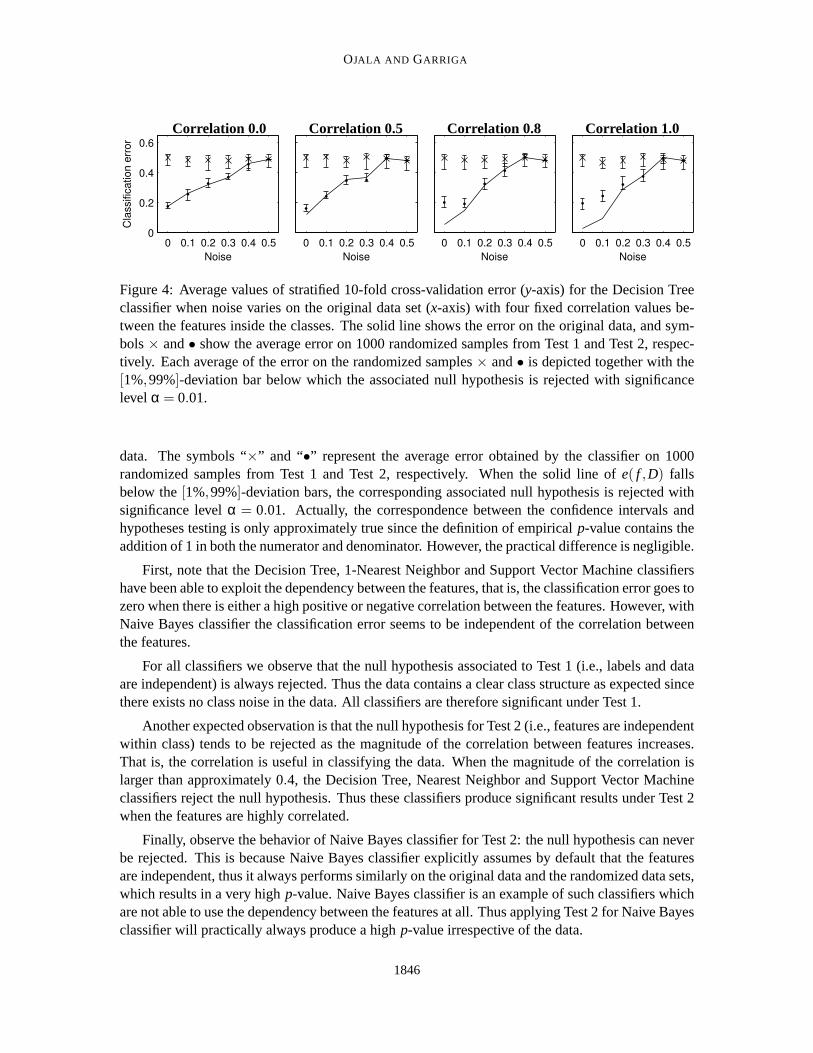
Figure 4: Average values of stratified 10-fold cross-validation error (y-axis) for the Decision Treeclassifier when noise varies on the original data set (x-axis) with four fixed correlation values be-tween the features inside the classes. The solid line shows the error on the original data, and sym-bols× and• show the average error on 1000 randomized samples from Test 1 and Test 2, respec-tively. Each average of the error on the randomized samples× and• is depicted together with the[1%,99%]-deviation bar below which the associated null hypothesis is rejected with significancelevel α = 0.01.

data. The symbols “×” and “•” represent the average error obtained by the classifier on 1000randomized samples from Test 1 and Test 2, respectively. When the solidline of e( f ,D) fallsbelow the[1%,99%]-deviation bars, the corresponding associated null hypothesis is rejected withsignificance levelα = 0.01. Actually, the correspondence between the confidence intervals andhypotheses testing is only approximately true since the definition of empiricalp-value contains theaddition of 1 in both the numerator and denominator. However, the practical difference is negligible.

First, note that the Decision Tree, 1-Nearest Neighbor and Support Vector Machine classifiershave been able to exploit the dependency between the features, that is, the classification error goes tozero when there is either a high positive or negative correlation between the features. However, withNaive Bayes classifier the classification error seems to be independent of the correlation betweenthe features.

For all classifiers we observe that the null hypothesis associated to Test1 (i.e., labels and dataare independent) is always rejected. Thus the data contains a clear classstructure as expected sincethere exists no class noise in the data. All classifiers are therefore significant under Test 1.

Another expected observation is that the null hypothesis for Test 2 (i.e., features are independentwithin class) tends to be rejected as the magnitude of the correlation between features increases.That is, the correlation is useful in classifying the data. When the magnitude of the correlation islarger than approximately 0.4, the Decision Tree, Nearest Neighbor and Support Vector Machineclassifiers reject the null hypothesis. Thus these classifiers produce significant results under Test 2when the features are highly correlated.

Finally, observe the behavior of Naive Bayes classifier for Test 2: thenull hypothesis can neverbe rejected. This is because Naive Bayes classifier explicitly assumes by default that the featuresare independent, thus it always performs similarly on the original data and the randomized data sets,which results in a very highp-value. Naive Bayes classifier is an example of such classifiers whichare not able to use the dependency between the features at all. Thus applying Test 2 for Naive Bayesclassifier will practically always produce a highp-value irrespective of the data.

1846


Finally, Figure 4 shows the behavior of the Decision Tree classifier when the noiset ∈ [0,0.5] isincreased on thex-axis. We also vary the correlationρ between the features per class and show theresults on four cases: zero correlation, 0.5, 0.8 and total correlation. We observe that as the noiseincreases thep-values tend to be larger. Therefore, it is more difficult to reject the null hypothesison very noisy data sets, that is, when the class structure is weak. This is true for both Test 1 andTest 2. However, Test 1 rejects the null hypothesis even if there is 30% of noise. This supports thefact already observed in related literature (Golland et al., 2005), that even a weak class structure iseasily regarded as significant with Test 1. Compared to this, Test 2 givesmore conservative results.

4.3 Power Analysis of Test 2

Thepowerof a statistical test is the probability that the test will reject the null hypothesis when thealternative hypothesis is true. The power of the test depends on how muchor how clearly the nullhypothesis is false. For example, in our case with Test 2, a classifier may rely solely on a strongdependency structure between some specific features in the classification,or it may use a weakfeature dependency to slightly improve the classification accuracy. Rejecting the null hypothesis ofTest 2 is much easier in the former than in the latter case. Note, however, thata strong dependencybetween the features is not always useful in separating the classes, asseen in Figure 2 with Irisdata set. So, the question with Test 2 is whether the classifier is exploiting some of the dependencystructure between the features in the data and how important such feature dependency is for theclassification of the data.

In general, the power of the test can only be analyzed in special cases.Nevertheless, suchanalysis can give some general idea of the power the test. Next, we present a formal power analysisin the particular case where we vary the correlation between the features that is useful in separatingthe classes from each other. Note, however, that there exist also othertypes of dependency thancorrelation. The amount of correlation is just easy to measure, thus being suitable for formal poweranalysis.

We present the power analysis on similar data as studied in Section 4.2. The results in theprevious subsection can be seen as informal power analysis. In summary, we observed that whenthe magnitude of the correlation in the data studied in Section 4.2 was larger than about 0.5 andthe classifier was exploiting the feature dependency, that is, a classifier different from Naive Bayes,Test 2 was able to reject the null hypothesis. However, based on the datait is clear that even smallercorrelations increased the class separation and were helpful in classifying the data but Test 2 couldnot regard such improvement as significant. The following analysis supports these observations.

Let the data setX consist ofn points with two features belonging to two classes,+1 and−1.Let a pointx∈ X be in classy= +1 with probability 0.5 and in classy= −1 with probability 0.5.Let the pointx ∈ X be sampled from two-dimensional normal distribution with mean(0,0), unitvariances and covarianceyρ whereρ ∈ [0,1] is a given parameter. Thus, in the first class,y= +1,the correlation between the two features is positive and in the second class,y= −1, it is negative.Compared to the data sets in Section 4.2, now the covariance changes between the classes, not themean vector. An optimal classifier assigns a pointx ∈ X to classy = +1 if x1x2 > 0 and to classy=−1 if x1x2 < 0, wherexi is thei-th feature of the vectorx.

The null hypothesis of Test 2 is that the classifier is not exploiting the dependency betweenthe features in classification. To alleviate the power analysis, we assume thatthe classifier is ableto find the optimal classification, that is, it assigns the pointx to class sgn(x1x2) where sgn(·) is

1847

OJALA AND GARRIGA

the signum function. If the classifier is not optimal, it will just decrease the power of the test.The nonoptimality of the classifier could be taken into account by introducing aprobability t forreporting a nonoptimal class label; this approach is used in the next subsection for power analysisof Test 1 but is left out here for simplicity in the analysis. Under this optimality scenario, theprobability of correctly classifying a sample is

Pr(sgn(x1x2) = y) =12

Pr(x1x2 > 0 | y=+1)+12

Pr(x1x2 < 0 | y=−1)

= Pr(x1x2 > 0 | y=+1) = 2∫ ∞

0

∫ ∞

0Pr(x1,x2)dx1dx2

= 2∫ ∞

0

∫ ∞

0

1

2π√

1−ρ2exp

[−x2

1−2ρx1x2+x22

2(1−ρ2)

]dx1dx2

=12+

1π

arcsinρ, (2)

where Pr(x1,x2) is just the standardized bivariate normal distribution. The null hypothesis corre-sponds to the case where the correlation parameter is zero,ρ = 0, that is, no feature dependencyexists. In that case, the probability of correctly classifying a sample is 1/2.

In our randomization approach, we are using classification error as the test statistic. Since weassume that the optimal classifier is given, we use all then points of the data setX for testingthe classifier and calculating the classification error. Under the null hypothesisH0 and under thealternative hypothesisH1 of Test 2, the classification errorse( f | H0) ande( f | H1) are distributedas follows:

n·e( f | H0)∼ Bin

(n,

12

)≈N

(n2,n4

),


(n,

12− 1

πarcsinρ

)≈N

(n2− n

πarcsinρ,

n4− n

π2 arcsin2 ρ),

where12 − 1

π arcsinρ is the probability of incorrectly classifying a sample by Equation (2). The nor-mal approximationN (np,np(1− p)) of a binomial distribution Bin(n, p) holds with good accuracywhennp> 5 andn(1− p)> 5. In our case, the approximation is valid ifn(1

2 − 1π arcsinρ)> 5. This

holds, for example, ifn≥ 20 andρ ≤ 0.7.Now the power of Test 2 for this generated data is the probability of rejectingthe null hypothesis

H0 of ρ = 0 with significance levelα when the alternative hypothesisH1 is that the correlationρ > 0. Note that we are implicitly assuming that the classifier is optimal, that is, we are excludingthe classifier quality from the power analysis. Thus, the power is the probability that e( f | H1) issmaller than 1−α of the errorse( f | H0) under the alternative hypothesisH1:

Power= Pr(

e( f | H1)< F−1e( f |H0)

(α))

≈ Pr

(12− 1

πarcsinρ+

√14n

− 1nπ2 arcsin2 ρ ·Z <

12+

12√

nΦ−1(α)

)

= Φ

2

√narcsinρ+πΦ−1(α)√

π2−4arcsin2 ρ

, (3)

1848


0.1

0.3

0.50.7

0.9

Number of rows

Corr

ela

tion

101

102

103

104

0

0.2

0.4

0.6

0.8

1

(a) α = 0.05

0.1

0.3

0.5

0.70.9

Number of rows

Corr

ela

tion

101

102

103

104

0

0.2

0.4

0.6

0.8

1

(b) α = 0.01

Figure 5: Contour plots of the statistical power of Test 2 as a function of thenumber of rowsn in thegenerated data set and the correlation parameterρ. Each solid line corresponds to a constant valueof the power that is given on top of the contour. The power values are calculated by Equation (3)for two different values of significance levelα.

whereFe( f |H0) is the cumulative distribution function ofe( f | H0), Z is a random variable followingstandard normal distribution andΦ is the cumulative distribution function of the standard normaldistribution. Note that we are using exactp-value instead of empiricalp-value, effectively leavingout the influence of variance by usingk randomized samples; see Fay et al. (2007) for analysis ofresampling risk of usingk samples. However, this has little effect to the power of the test. When thecorrelationρ = 0, the power isα, that is, when the null hypothesis is true, it is rejected incorrectlyaboutα of the times. Therefore,α is really the significance level of the tests.

In Figure 5 we present contour plots of the statistical power in Equation (3)for different valuesof the two varying parameters. As expected, the higher the correlationρ and the number of rowsn are, the higher the statistical power of Test 2 is. For example, if the data setcontains about 1000rows, we can infer with 90% probability that the classifier is exploiting the feature dependency ofapproximately a correlation of 0.2 in the data. The results are also in line with the results fromSection 4.2 although the studied data sets are slightly different. When the significance level used isα = 0.01 we can infer that the classifier is exploiting the feature dependency of correlation largerthan 0.4 approximately 90% of the times when the data set has 200 rows.

Notice that if we had not considered an “optimal” classifier, that is, if we hadintroduced aprobability t of assigning each observation to the incorrect label, then Equation (3) would dependon three parameters. In that case, the highert, the smaller is the power of the test; however, fora fixed t we still would observe the same behaviour as in the contourplots above: the higher thecorrelationρ and the larger then, the higher is the statistical power of Test 2. The error parametertis taken into account in the next section, where the power analysis of Test1 does not depend onρbetween the features.

1849

OJALA AND GARRIGA

4.4 Power Analysis of Test 1

Let the data setX consist ofn observations belonging to two different classes with equal probability.We assume that we have a classifierf whose error rate ist ∈ [0,1], that is, the classifier assigns eachobservation to the correct class with probability 1− t. Another way to see this is that the classifierf is optimal but the original class label of each point is erroneous with probability t. We performpower analysis of Test 1 for this general form of data.

Note that the results in Section 4.2 can be seen as informal power analysis ofTest 1 on similarsetting as studied here. The results in Figure 4 can be summarized as follows.When the error ratewas smaller thant < 0.4, Test 1 was able to reject the null hypotheses. Note, however, that theerrorratet used in this section is not directly comparable to the error rate used in Section 4.2.

The power analysis of Test 1 proceeds similarly as in the previous subsection for Test 2. Underthe null hypothesisH0 and under the alternative hypothesisH1 of Test 1, the classification errorse( f | H0) ande( f | H1) are distributed as follows:


(n,

12

)≈N

(n2,n4

),

n·e( f | H1)∼ Bin(n, t)≈N (nt,nt(1− t)) .

The null hypothesisH0 assumes that there is no connection between the data and the class labelsthus the probability of incorrect classification is 1/2 as the classes are equally probable. Note thatthe null hypothesis corresponds to the case where the error rate of the classifier f is t = 1/2.

Now the power of Test 1 is the probability of rejecting the null hypothesisH0 with significancelevel α when the alternative hypothesisH1 is true, that is,

Power= Pr(

e( f | H1)< F−1e( f |H0)

(α))

≈ Pr

(t +

√t(1− t)

nZ <

12+

12√

nΦ−1(α)

)

= Φ

((1−2t)

√n+Φ−1(α)

2√

t(1− t)

), (4)

where the same notation as in the previous subsection is used. First, note thatwhen the null hypoth-esis is true, that is,t = 1/2, the power of Test 1 calculated by Equation (4) equals the significancelevel α as it should.

In Figure 6 we present contour plots of the statistical power of Test 1 calculated by Equation (4)for different values of parameters. As expected, when the number of observationsn increases or theerror ratet decreases, the power increases. Furthermore, the larger the significance levelα is, thelarger the power of Test 1 is. When the parameter values areα = 0.01, n = 200 andt = 0.4, thepower of Test 1 is about 0.7 that is comparable to the results in Section 4.2.

In this section, we analyzed the behaviour and the power of the tests. Note that although we usedcorrelation as the only type of dependency between features in this section, there exist also otherforms of dependency that the classifier can exploit. As conclusions fromthe power analysis, themore rows the data set has, the easier we can infer that the classifier is using the feature dependencyor some other properties in the data.

1850


0.1

0.3

0.5

0.7

0.9

Number of rows

Pro

babili

ty o

f m

iscla

ssific

ation

101

102

103

104

0

0.1

0.2

0.3

0.4

0.5

(a) α = 0.05

0.1

0.3

0.5

0.7

0.9

Number of rows

Pro

babili

ty o

f m

iscla

ssific

ation

101

102

103

104

0

0.1

0.2

0.3

0.4

0.5

(b) α = 0.01

Figure 6: Contour plots of the statistical power of Test 1 as a function of thenumber of rowsn inthe generated data set and the probability of misclassificationt. Each solid line corresponds to aconstant value of the power that is given on top of the contour. The power values are calculated byEquation (4) for two different values of significance levelα.

5. Empirical Results

In this section, we give extensive empirical results on 33 various real data sets from UCI machinelearning repository (Asuncion and Newman, 2007). Basic characteristics of the data sets are de-scribed in Table 2. The data sets are divided into three categories based on their size: small, mediumand large. Some data sets contain only nominal or numeric features whereassome data sets containboth kind of features (mixed). About one-third of the data sets contain alsomissing values. Noticethat in most data sets the features are measured in different scales, thus itis not sensible to swap thevalues between different features. This justifies why it is only reasonable to consider column-wisepermutations, and why some recent data mining randomization methods (Gionis etal., 2007; Ojalaet al., 2009; Chen et al., 2005) are not generally applicable in assessingclassification results.

In the experiments we use Weka 3.6 data mining software (Witten and Frank, 2005) that containsopen source Java implementations of many classification algorithms. We use four different typesof classification algorithms with the default parameters: Decision Tree, Naive Bayes, 1-NearestNeighbor and Support Vector Machine classifier. The Decision Tree classifier is similar to C4.5algorithm. The default kernel used with Support Vector Machine is linear.Missing values and thecombination of nominal and numerical values are given as such as the inputfor the classifiers; thedefault approaches in Weka of the classifiers are used to handle these cases. Notice that tuning theparameters of these algorithms is not in the scope of this paper; our objective is to show the behaviorof the discussedp-values for some selected classifiers on various data sets.

We use different classification procedures and the number of randomized data sets for eachof the different size categories of the data sets (small, medium and large). For small data sets,we use stratified 10-fold cross-validation error as the statistic and 1000 randomized data sets forcalculating the empiricalp-values. For medium-sized data sets, we use the same stratified 10-foldcross-validation error and 100 randomized data sets. Finally, for large data sets, we divide the data

1851

OJALA AND GARRIGA

Data Set Rows Features Classes Missing Domain

Sm

all

Audiology 226 70 24 2.0% nominalAutos 205 25 6 1.2% mixedBreast 286 9 2 0.3% nominalGlass 214 9 6 No numericHepatitis 155 19 2 5.7% mixedIonosphere 351 34 2 No numericIris 150 4 3 No numericLymph 148 18 4 No mixedPromoters 106 57 2 No nominalSegment 210 19 7 No numericSonar 208 60 2 No numericSpect 267 22 2 No nominalTumor 339 17 21 3.9% nominalVotes 435 16 2 5.6% nominalZoo 101 17 7 No mixed

Med

ium

Abalone 4177 8 28 No mixedAnneal 898 38 5 65.0% mixedBalance 625 4 3 No numericCar 1728 6 4 No nominalGerman 1000 20 2 No mixedMushroom 8124 22 2 1.4% nominalMusk 6598 166 2 No numericPima 768 8 2 No numericSatellite 6435 36 6 No numericSpam 4601 57 2 No numericSplice 3190 60 3 No nominalTic-tac-toe 958 9 2 No nominalYeast 1484 8 10 No numeric

Larg

e

Adult 48842 15 2 0.9% mixedChess 28056 6 18 No mixedConnect-4 67557 42 3 No nominalLetter 20000 16 26 No numericShuttle 58000 9 7 No numeric

Table 2: Summary of 33 selected data sets from UCI machine learning repository (Asuncion andNewman, 2007). The data sets are divided into three categories based ontheir size: small, mediumand large.

1852


set into training set with 10 000 random rows and to test set with the rest of the rows. We use 100randomized data sets for calculating the empiricalp-values with large data sets. The reason for thesmaller number of randomized samples for medium and large data sets is mainly computation time.However, 100 samples is usually enough for statistical inference. Furthermore, as seen in Section 4the power of the tests is greater when the data sets have more rows, that is, with large data sets it iseasier to reject the null-hypotheses, supporting the need of fewer randomized samples in hypothesistesting.

Since the original classification error is not a stable result due to the randomness in trainingthe classifier and dividing the data set into test and train data, we perform the same classificationprocedure ten times for the original data sets and calculate an empiricalp-value for each of the tenresults. This was described in Section 3.2. We give the average value of these empiricalp-values aswell as the average value and the standard deviation of the original classification errors.

As we are testing multiple hypotheses simultaneously, we need to correct for multiple compar-isons. We apply the approach by Benjamini and Hochberg (1995) to control the false discovery rate(FDR), that is, the expected proportion of results incorrectly regardedas significant. In the exper-iments, we restrict the false discovery rate belowα = 0.05 separately for Test 1 and Test 2. In theBenjamini-Hochberg approach, ifp1, . . . , pm are the original empiricalp-values in increasing order,the resultsp1, . . . , pl are regarded as significant wherel is the largest value such thatpl ≤ l

mα.The significance testing results for the Decision Tree classifier are givenin Table 3, for Naive

Bayes in Table 4, for 1-Nearest Neighbor classifier in Table 5 and finallyfor Support Vector Ma-chine classifier in Table 6. The mean and the standard deviation of the 10 original classificationerrors are given as well as the mean and standard deviation of the errors on the 1000 or 100 ran-domized samples with Test 1 and Test 2. The empiricalp-values corresponding to nonsignificantresults, when the false discovery rate is restricted below 0.05, are in boldface in the tables. With allclassifiers, the largest significant empiricalp-value was 0.01. The smallest non-significantp-valueswere 0.03 with Decision Tree and 1-Nearest Neighbor classifiers, 0.08 with Naive Bayes classifierand 0.19 with Support Vector Machine classifier.

The results for the traditional permutation method Test 1 show that the classification errors withmost data sets are regarded as significant. These results show that the data sets contain clear classstructure. However, they do not give any additional insight for understanding the class structure inthe data sets.

There are two reasons why the simple permutation test, Test 1, regards the class structure ofthe data sets as significant. Firstly, most of the data sets that are publicly available, as all thedata sets used in this paper, have already passed some quality checks, that is, someone has alreadyfound some interesting structure in them. Secondly, and as a more important reason, the traditionalpermutation tests easily regard the results as significant even if there is only aslight class structurepresent because in the corresponding permuted data sets there is no class structure, especially if theoriginal data set is large.

Furthermore, the few results which were regarded as nonsignificant withTest 1 are with suchclassifiers that have not performed well on the data. That is, the other classifiers have producedsmaller classification errors on the same data sets, and, in contrast, these results are regarded assignificant.

Next, we consider the results for permuting the features inside each class,that is, Test 2. Theresults show that there are actually now almost equal amount of nonsignificant and significant resultswith respect to Test 2. This means that in many data sets the original structureinside the classes is

1853

OJALA AND GARRIGA

Decision Tree

Original Test 1 Test 2

Data Set Err. (Std) Err. (Std) p-val. Err. (Std) p-val.S

mal

lAudiology 0.22 (0.01) 0.82 (0.03) 0.001 0.23 (0.02)0.482Autos 0.19 (0.01) 0.76 (0.04) 0.001 0.38 (0.04) 0.001Breast 0.26 (0.01) 0.30 (0.00) 0.001 0.29 (0.02)0.116Glass 0.33 (0.02) 0.72 (0.03) 0.001 0.34 (0.03)0.457Hepatitis 0.22 (0.02) 0.23 (0.02)0.319 0.15 (0.03) 0.955Ionosphere 0.10 (0.01) 0.38 (0.02) 0.001 0.07 (0.01)0.964Iris 0.05 (0.01) 0.67 (0.03) 0.001 0.05 (0.01)0.765Lymph 0.22 (0.02) 0.51 (0.05) 0.001 0.23 (0.04)0.437Promoters 0.21 (0.04) 0.50 (0.06) 0.002 0.22 (0.05)0.377Segment 0.13 (0.02) 0.86 (0.03) 0.001 0.17 (0.02)0.132Sonar 0.27 (0.02) 0.49 (0.03) 0.001 0.27 (0.03)0.507Spect 0.19 (0.01) 0.22 (0.01) 0.004 0.15 (0.02)0.966Tumor 0.58 (0.01) 0.82 (0.02) 0.001 0.60 (0.02)0.138Votes 0.03 (0.00) 0.42 (0.02) 0.001 0.03 (0.01)0.791Zoo 0.07 (0.01) 0.64 (0.03) 0.001 0.07 (0.01)0.593

Med

ium

Abalone 0.79 (0.01) 0.89 (0.00) 0.01 0.67 (0.01)1.00Anneal 0.07 (0.01) 0.24 (0.00) 0.01 0.13 (0.01) 0.01Balance 0.22 (0.01) 0.55 (0.02) 0.01 0.29 (0.02) 0.01Car 0.08 (0.00) 0.30 (0.00) 0.01 0.26 (0.01) 0.01German 0.29 (0.01) 0.32 (0.01) 0.01 0.28 (0.01)0.66Mushroom 0.00 (0.00) 0.50 (0.01) 0.01 0.01 (0.00) 0.01Musk 0.03 (0.00) 0.16 (0.00) 0.01 0.09 (0.00) 0.01Pima 0.25 (0.01) 0.35 (0.01) 0.01 0.24 (0.01)0.67Satellite 0.14 (0.00) 0.81 (0.00) 0.01 0.07 (0.00)1.00Spam 0.07 (0.00) 0.40 (0.00) 0.01 0.06 (0.00)1.00Splice 0.06 (0.00) 0.60 (0.01) 0.01 0.07 (0.01) 0.01Tic-tac-toe 0.15 (0.01) 0.36 (0.01) 0.01 0.30 (0.01) 0.01Yeast 0.44 (0.01) 0.76 (0.01) 0.01 0.47 (0.01)0.03

Larg

e

Adult 0.00 (0.00) 0.24 (0.00) 0.01 0.00 (0.00)1.00Chess 0.46 (0.00) 0.89 (0.00) 0.01 0.77 (0.00) 0.01Connect-4 0.25 (0.00) 0.34 (0.00) 0.01 0.33 (0.00) 0.01Letter 0.16 (0.01) 0.96 (0.00) 0.01 0.38 (0.01) 0.01Shuttle 0.00 (0.00) 0.21 (0.00) 0.01 0.01 (0.00) 0.01

Table 3: Classification errors and empiricalp-values obtained with Decision Tree classifier forTest 1 and Test 2. The empiricalp-values are calculated over 1000 randomized samples for smalldata sets and over 100 randomized samples for medium and large data sets. Classification on theoriginal data is repeated ten times. In the table, the average values and standard deviations of theclassification errors are given. Boldp-values correspond to nonsignificant results when the falsediscovery rate is restricted below 0.05 with Benjamini and Hochberg (1995)approach.

1854


Naive Bayes



mal

lAudiology 0.27 (0.00) 0.79 (0.03) 0.001 0.26 (0.01)0.869Autos 0.43 (0.01) 0.79 (0.04) 0.001 0.22 (0.02)1.000Breast 0.27 (0.01) 0.33 (0.02) 0.001 0.24 (0.02)0.959Glass 0.52 (0.02) 0.81 (0.05) 0.001 0.45 (0.02)0.994Hepatitis 0.16 (0.01) 0.30 (0.05) 0.001 0.09 (0.02)1.000Ionosphere 0.17 (0.00) 0.46 (0.03) 0.001 0.01 (0.01)1.000Iris 0.05 (0.01) 0.67 (0.05) 0.001 0.01 (0.01)0.999Lymph 0.16 (0.01) 0.53 (0.05) 0.001 0.11 (0.02)0.995Promoters 0.08 (0.01) 0.50 (0.06) 0.001 0.07 (0.02)0.746Segment 0.21 (0.01) 0.86 (0.03) 0.001 0.13 (0.01)1.000Sonar 0.32 (0.01) 0.50 (0.04) 0.001 0.13 (0.02)1.000Spect 0.21 (0.01) 0.25 (0.03)0.077 0.07 (0.01) 1.000Tumor 0.50 (0.01) 0.81 (0.02) 0.001 0.49 (0.02)0.751Votes 0.10 (0.00) 0.44 (0.02) 0.001 0.00 (0.00)1.000Zoo 0.03 (0.00) 0.81 (0.05) 0.001 0.03 (0.01)0.541

Med

ium

Abalone 0.76 (0.00) 0.88 (0.01) 0.01 0.56 (0.01)1.00Anneal 0.35 (0.01) 0.36 (0.04) 0.65 0.31 (0.01) 1.00Balance 0.09 (0.00) 0.54 (0.02) 0.01 0.24 (0.01) 0.01Car 0.14 (0.00) 0.30 (0.00) 0.01 0.24 (0.01) 0.01German 0.25 (0.00) 0.33 (0.01) 0.01 0.23 (0.01)1.00Mushroom 0.04 (0.00) 0.50 (0.01) 0.01 0.00 (0.00)1.00Musk 0.16 (0.00) 0.34 (0.06) 0.01 0.02 (0.00)1.00Pima 0.24 (0.00) 0.37 (0.01) 0.01 0.22 (0.01)0.99Satellite 0.20 (0.00) 0.80 (0.02) 0.01 0.00 (0.00)1.00Spam 0.20 (0.00) 0.49 (0.05) 0.01 0.10 (0.00)1.00Splice 0.05 (0.00) 0.53 (0.01) 0.01 0.03 (0.00)1.00Tic-tac-toe 0.30 (0.00) 0.35 (0.01) 0.01 0.28 (0.01)1.00Yeast 0.42 (0.00) 0.71 (0.01) 0.01 0.42 (0.01)0.36

Larg

e

Adult 0.02 (0.00) 0.24 (0.01) 0.01 0.01 (0.00)0.96Chess 0.66 (0.00) 0.84 (0.00) 0.01 0.70 (0.00) 0.01Connect-4 0.28 (0.00) 0.34 (0.00) 0.01 0.29 (0.00)0.19Letter 0.36 (0.00) 0.96 (0.00) 0.01 0.26 (0.00)1.00Shuttle 0.10 (0.01) 0.47 (0.24) 0.01 0.04 (0.01)1.00

Table 4: Classification errors and empiricalp-values obtained with Naive Bayes classifier for Test 1and Test 2. The empiricalp-values are calculated over 1000 randomized samples for small data setsand over 100 randomized samples for medium and large data sets. Classification on the original datais repeated ten times. In the table, the average values and standard deviations of the classificationerrors are given. Boldp-values correspond to nonsignificant results when the false discoveryrate isrestricted below 0.05 with Benjamini and Hochberg (1995) approach.

1855

OJALA AND GARRIGA

1-Nearest Neighbor



mal

lAudiology 0.26 (0.01) 0.86 (0.03) 0.001 0.32 (0.03)0.030Autos 0.26 (0.01) 0.77 (0.03) 0.001 0.45 (0.03) 0.001Breast 0.31 (0.02) 0.41 (0.03) 0.007 0.32 (0.03)0.324Glass 0.30 (0.01) 0.74 (0.04) 0.001 0.42 (0.03) 0.001Hepatitis 0.19 (0.01) 0.33 (0.04) 0.002 0.14 (0.03)0.970Ionosphere 0.13 (0.00) 0.46 (0.03) 0.001 0.26 (0.01) 0.001Iris 0.05 (0.00) 0.66 (0.05) 0.001 0.02 (0.01)0.962Lymph 0.18 (0.02) 0.53 (0.04) 0.001 0.20 (0.03)0.307Promoters 0.19 (0.02) 0.50 (0.06) 0.001 0.26 (0.04)0.083Segment 0.14 (0.01) 0.86 (0.03) 0.001 0.15 (0.02)0.266Sonar 0.13 (0.01) 0.50 (0.04) 0.001 0.27 (0.03) 0.001Spect 0.24 (0.02) 0.32 (0.04) 0.011 0.18 (0.02)0.970Tumor 0.66 (0.02) 0.88 (0.02) 0.001 0.62 (0.02)0.860Votes 0.08 (0.01) 0.47 (0.03) 0.001 0.01 (0.00)1.000Zoo 0.03 (0.01) 0.75 (0.05) 0.001 0.04 (0.02)0.333

Med

ium

Abalone 0.80 (0.00) 0.90 (0.00) 0.01 0.68 (0.01)1.00Anneal 0.05 (0.00) 0.40 (0.02) 0.01 0.08 (0.01) 0.01Balance 0.20 (0.01) 0.57 (0.02) 0.01 0.35 (0.02) 0.01Car 0.22 (0.01) 0.41 (0.05) 0.01 0.29 (0.01) 0.01German 0.28 (0.01) 0.42 (0.02) 0.01 0.33 (0.02) 0.01Mushroom 0.00 (0.00) 0.50 (0.01) 0.01 0.01 (0.00) 0.01Musk 0.04 (0.00) 0.26 (0.00) 0.01 0.53 (0.01) 0.01Pima 0.29 (0.00) 0.45 (0.02) 0.01 0.27 (0.02)0.88Satellite 0.10 (0.00) 0.81 (0.01) 0.01 0.01 (0.00)1.00Spam 0.09 (0.00) 0.48 (0.01) 0.01 0.09 (0.00)0.31Splice 0.24 (0.01) 0.61 (0.01) 0.01 0.30 (0.01) 0.01Tic-tac-toe 0.21 (0.02) 0.44 (0.07) 0.01 0.38 (0.02) 0.01Yeast 0.47 (0.01) 0.78 (0.01) 0.01 0.52 (0.01) 0.01

Larg

e

Adult 0.02 (0.00) 0.36 (0.00) 0.01 0.01 (0.00)1.00Chess 0.48 (0.00) 0.90 (0.00) 0.01 0.80 (0.00) 0.01Connect-4 0.34 (0.00) 0.50 (0.00) 0.01 0.43 (0.00) 0.01Letter 0.06 (0.00) 0.96 (0.00) 0.01 0.46 (0.00) 0.01Shuttle 0.00 (0.00) 0.36 (0.00) 0.01 0.02 (0.00) 0.01

Table 5: Classification errors and empiricalp-values obtained with 1-Nearest Neighbor classifierfor Test 1 and Test 2. The empiricalp-values are calculated over 1000 randomized samples forsmall data sets and over 100 randomized samples for medium and large data sets. Classification onthe original data is repeated ten times. In the table, the average values and standard deviations ofthe classification errors are given. Boldp-values correspond to nonsignificant results when the falsediscovery rate is restricted below 0.05 with Benjamini and Hochberg (1995)approach.

1856


Support Vector Machine



mal

lAudiology 0.20 (0.01) 0.83 (0.03) 0.001 0.20 (0.02)0.443Autos 0.30 (0.02) 0.73 (0.04) 0.001 0.26 (0.03)0.873Breast 0.30 (0.01) 0.31 (0.01)0.191 0.25 (0.02) 0.970Glass 0.42 (0.01) 0.65 (0.03) 0.001 0.43 (0.02)0.363Hepatitis 0.14 (0.01) 0.21 (0.00) 0.001 0.08 (0.02)0.999Ionosphere 0.12 (0.01) 0.37 (0.01) 0.001 0.08 (0.01)0.995Iris 0.04 (0.01) 0.67 (0.05) 0.001 0.02 (0.01)0.990Lymph 0.14 (0.01) 0.51 (0.05) 0.001 0.12 (0.03)0.686Promoters 0.09 (0.01) 0.50 (0.06) 0.001 0.10 (0.03)0.455Segment 0.12 (0.01) 0.86 (0.03) 0.001 0.12 (0.01)0.529Sonar 0.23 (0.02) 0.49 (0.04) 0.001 0.10 (0.02)0.999Spect 0.17 (0.01) 0.21 (0.00) 0.001 0.08 (0.02)1.000Tumor 0.53 (0.01) 0.77 (0.01) 0.001 0.53 (0.02)0.406Votes 0.04 (0.00) 0.39 (0.01) 0.001 0.01 (0.00)1.000Zoo 0.04 (0.00) 0.66 (0.04) 0.001 0.04 (0.01)0.666

Med

ium

Abalone 0.75 (0.00) 0.84 (0.00) 0.01 0.57 (0.01)1.00Anneal 0.15 (0.00) 0.24 (0.00) 0.01 0.14 (0.01)0.78Balance 0.12 (0.01) 0.54 (0.03) 0.01 0.25 (0.01) 0.01Car 0.06 (0.00) 0.30 (0.00) 0.01 0.25 (0.01) 0.01German 0.25 (0.00) 0.30 (0.00) 0.01 0.22 (0.01)1.00Mushroom 0.00 (0.00) 0.50 (0.01) 0.01 0.00 (0.00) 0.01Musk 0.05 (0.00) 0.15 (0.00) 0.01 0.01 (0.00)1.00Pima 0.23 (0.00) 0.35 (0.00) 0.01 0.21 (0.01)1.00Satellite 0.13 (0.00) 0.77 (0.00) 0.01 0.00 (0.00)1.00Spam 0.10 (0.00) 0.39 (0.00) 0.01 0.04 (0.00)1.00Splice 0.07 (0.00) 0.48 (0.00) 0.01 0.06 (0.01)0.99Tic-tac-toe 0.02 (0.00) 0.37 (0.01) 0.01 0.30 (0.01) 0.01Yeast 0.43 (0.00) 0.69 (0.01) 0.01 0.42 (0.01)0.72

Larg

e

Adult 0.00 (0.00) 0.24 (0.00) 0.01 0.00 (0.00)1.00Chess 0.66 (0.01) 0.85 (0.00) 0.01 0.72 (0.00) 0.01Connect-4 0.24 (0.00) 0.45 (0.07) 0.01 0.29 (0.00) 0.01Letter 0.19 (0.01) 0.96 (0.00) 0.01 0.32 (0.00) 0.01Shuttle 0.04 (0.01) 0.21 (0.00) 0.01 0.04 (0.00)0.45

Table 6: Classification errors and empiricalp-values for the Support Vector Machine classifier forTest 1 and Test 2. The empiricalp-values are calculated over 1000 randomized samples for smalldata sets and over 100 randomized samples for medium and large data sets. Classification on theoriginal data is repeated ten times. In the table, the average values and standard deviations of theclassification errors are given. Boldp-values correspond to nonsignificant results when the falsediscovery rate is restricted below 0.05 with Benjamini and Hochberg (1995)approach.

1857

OJALA AND GARRIGA

pretty simple, or it is not used by the classification algorithm. That is, the classes differ from eachother, from the point of view of the classifiers, mainly due to their differentvalue distributions ofthe features and not due to some dependency between the features. Thus, in many data sets the classstructure is explained by considering the features independently of eachother.

The results with Naive Bayes classifier are in line with the analysis in Section 4.2. That is,practically all of the results are nonsignificant with Naive Bayes with Test 2as it explicitly assumesindependence of the features. However, there are three data sets where the results are regardedas significant with Test 2: Balance, Car and Chess. These three data sets seem to contain a goodbalance between the features that makes the Naive Bayes classifier to perform better on the originaldata than on the randomized data sets. That is, each instance contains usually at least one featurewhich makes the classification easy whereas in the randomized data sets thereare instances that donot have separating values in any of the features. Thus, applying Test2 to Naive Bayes classifierdoes not tell whether the classifier uses the interdependency between thefeatures but whether thedata are such that usually at least one feature in each instance has a clear separating value.

Compared to the other three classifiers, Naive Bayes is having both better and worse perfor-mance with all kind of data sets. Surprisingly, however, Naive Bayes is performing better also in afew such cases where the other classifiers are exploiting the feature dependency. For example, withdata sets Splice and Yeast the Naive Bayes classifier has the best accuracy although the DecisionTree and 1-Nearest Neighbor classifiers are significant with Test 2. Thus if a classifier is usingthe feature dependency in the classification, it does not directly imply that some other classifiercould not do better without using the dependency. In such case, however, it is likely that neitherof the classifiers are optimal and we could obtain even better performance by combining the goodproperties of both the classifiers.

In the rest of this section, we will consider only the three other classifiers,namely Decision Tree,1-Nearest Neighbor and Support Vector Machine classifiers. Thereis a clear difference between thesmall and large data sets with these classifiers. The results with Test 2 for small data sets are almostall nonsignificant whereas the results for large data sets are almost all significant. Only the Adultdata set from large data sets seems to contain simple class structure. Actually,the Decision Tree andSupport Vector Machine classifiers are able to classify correctly all the test samples on the originalAdult data set as well as on the randomized versions of the Adult data set of Test 2. The results withthe studied small UCI data sets are understandable, as many of them are known to contain fairlysimple structure.

The results with the three classifiers are close to each other with all tests. Surprisingly, however,1-Nearest Neighbor classifier has been able to use the interdependency between the features themost, that is, it contains the most of small, significantp-values with Test 2. However, other morecomplex classifiers could be able to find more data sets where the dependency between the featuresis useful in classification.

Let us now study the results with Test 2 in more detail. Consider the well-knownIris data setthat contains measurements of three different species of iris flowers from four features: the lengthand the width of sepal and petal. It turns out that the classes are almost linearly separable giventhe length of petal or given the width of petal. Although there is a high positivelinear correlationbetween the length and width of petal, it is not important for the classification result as both featurescan explain the classes by themselves.

Actually, observe that for the Iris data set with Test 2, the classification error on the random-ized samples is even smaller than in the original data set. This phenomenon is explained by the

1858


positive linear correlation between the length and the width of petal, which disappears after therandomizations, as seen in Figure 2 in Section 3.1. Randomizations eliminate most of the rowscontaining extreme values for both of the features inside the classes. Thus, the classifiers do not usethe dependency between these two features, as their correlation does not help in classifying the Irisdata. When this positive correlation is eliminated per classes, the separation between the classesincreases, and therefore, the classification accuracy is improved.

For most of the data sets where the empiricalp-values are very high for the null hypothesis ofTest 2, there are either outliers inside the classes or positive correlation between some features thatis not used in the classification as it does not help in separating the classes.For example, the data setVotes contains congressional “yes” and “no” voting records from republicans and democrats. Thereare few voting cases where the opinion of the voter clearly reveals the political views. However,there are some outliers, that is, people who have behaved more like democrats although they arerepublicans, or vice versa, that vanish after randomization. Nevertheless, these reasons do notremove the fact that the features independently classify the voting records.

Finally, we discuss the results for the Balance data set. With all classifiers theclassificationresults of the Balance data set are significant under the null hypothesis of Test 2, that is, the clas-sifiers have exploited the dependency between the features. The structure of the data supportsthis: The data contains four features of a balance scale: left-weight, left-distance, right-weight andright-distance. The scale is in balance if left-weight times left-distance equalsright-weight timesright-distance. There are three classes: the scale tips to the left, to the right,or is in balance. It isclear that the dependency between the features is necessary for correct classification result.

Note however, that understanding the structure inside the data sets wherethe classification re-sults are regarded as significant under the null hypothesis of Test 2 requires more study, that is,we just know that the features do not explain the class structure independently. Analyzing the de-pendency structure of the features is then a further task. But as seen,the null hypothesis of Test 2explains about half of the good classification results in the 33 data sets.

We conclude the experiments with a summary about the running times of the methods. We usedMATLAB for producing the randomized data sets and Weka for performingthe classification on a2.2 GHz Opteron with 4 GB of main memory. The running times of producing one randomizationof each data set and the running times of calculating the classification errorson the original data setsand on the randomized data sets are given in Table 7. The running times of producing the random-ized data sets are negligible compared to the running times of calculating the classification errorsof the data sets, that is, training and testing the classifiers. There is, however, a small differencebetween the running times of obtaining the classification errors on the originaland the randomizeddata sets. Usually, the classification is a little bit faster on the original data set than on the random-ized data sets. Furthermore, the classification on randomized data sets of Test 2 is usually fasterthan on randomized data sets of Test 1. The reason is that it is harder to teach a classifier on arandomized data set which has usually a weaker class structure than the original data set. Amongthe two randomization tests, Test 2 generally preserves the original class structure the most becauseit preserves some connection between the data and the class labels.

6. Conclusions

We have considered the problem of assessing the classifier performance with permutation tests inthe statistical framework of hypothesis testing. We have described two different null hypotheses and

1859

OJALA AND GARRIGA

Rand. Decision Tree Naive Bayes 1-Near. Neighbor Supp. Vect. Mach.

Data Set T1 T2 Or. T1 T2 Or. T1 T2 Or. T1 T2 Or. T1 T2

Sm

all

Audiology 0.0 0.0 1.9 2.0 1.5 1.8 1.8 1.8 1.8 1.5 1.8 39 36 36Autos 0.0 0.0 0.5 0.5 0.5 0.5 0.4 0.4 0.5 0.4 0.4 3.2 2.2 2.3Breast 0.0 0.0 0.5 0.4 0.4 0.4 0.4 0.4 0.5 0.5 0.4 1.1 0.9 0.7Glass 0.0 0.0 0.4 0.4 0.3 0.3 0.3 0.2 0.3 0.2 0.2 2.4 2.3 2.3Hepatitis 0.0 0.0 0.4 0.3 0.3 0.3 0.3 0.2 0.3 0.3 0.3 0.5 0.4 0.4Ionosphere 0.0 0.0 1.2 1.0 0.9 0.8 0.7 0.7 0.9 0.8 0.9 1.2 1.3 1.0Iris 0.0 0.0 0.2 0.2 0.1 0.2 0.1 0.1 0.2 0.1 0.1 0.5 0.6 0.4Lymph 0.0 0.0 0.4 0.3 0.3 0.3 0.3 0.3 0.3 0.3 0.3 1.2 1.2 1.1Promoters 0.0 0.0 0.8 0.6 0.7 0.6 0.6 0.6 0.6 0.6 0.6 1.0 0.9 0.8Segment 0.0 0.0 0.5 0.6 0.4 0.4 0.3 0.3 0.4 0.3 0.4 3.6 2.4 2.3Sonar 0.0 0.0 1.2 0.9 1.1 0.9 0.7 0.7 0.9 0.9 0.9 1.1 1.1 0.9Spect 0.0 0.0 0.7 0.6 0.6 0.6 0.8 0.6 0.8 0.6 0.6 0.8 0.8 0.7Tumor 0.0 0.0 0.9 0.8 0.8 0.8 0.7 0.6 0.8 0.8 0.8 30 21 26Votes 0.0 0.0 1.0 0.8 0.7 0.9 0.9 0.7 1.0 0.9 0.8 1.2 1.1 1.1Zoo 0.0 0.0 0.2 0.2 0.2 0.2 0.2 0.2 0.2 0.2 0.2 3.1 3.1 2.6

Med

ium

Abalone 0.0 0.0 7.0 8.9 6.7 3.1 3.0 3.0 7.6 7.8 7.8 54 78 60Anneal 0.0 0.0 2.9 2.9 2.9 2.3 2.3 2.3 3.1 3.1 3.2 4.7 9.3 4.6Balance 0.0 0.0 0.5 0.5 0.5 0.4 0.3 0.4 0.5 0.5 0.4 0.9 1.0 0.8Car 0.0 0.0 1.4 1.5 1.4 1.4 1.4 1.3 1.8 1.8 1.7 5.1 8.0 7.7German 0.0 0.0 1.8 1.5 1.5 1.6 1.2 1.5 2.0 2.1 2.1 9.4 6.3 9.8Mushroom 0.0 0.0 21 24 21 20 21 20 68 70 70 60 1197 26Musk 0.0 0.2 130 110 176 55 63 80 230 309 318 502 5816 86Pima 0.0 0.0 0.8 0.7 0.9 0.7 0.7 0.5 0.8 0.7 0.8 0.9 0.8 0.9Satellite 0.0 0.0 26 128 21 13 14 14 59 62 81 19 157 15Spam 0.0 0.1 32 16 23 14 14 14 39 56 56 21 38 17Splice 0.0 0.0 17 17 16 15 16 15 36 28 28 87 1922 95Tic-tac-toe 0.0 0.0 1.0 1.0 1.0 1.0 1.0 1.0 1.1 1.1 1.2 3.1 3.5 6.6Yeast 0.0 0.0 1.7 2.2 1.6 1.3 1.0 1.3 1.4 1.4 1.7 5.2 5.3 4.9

Larg

e

Adult 0.0 0.4 55 60 58 56 62 67 315 325 304 77 134 63Chess 0.0 0.1 71 57 54 45 54 59 131 105 111 93 89 102Connect-4 0.0 0.9 379 380 292 387 391 291 1161 1297 1285 975 5581066Letter 0.0 0.1 37 45 42 32 45 34 95 103 99 43 50 45Shuttle 0.0 0.2 176 139 142 141 143 138 339 419 319 149 170 140

Table 7: Average running times in seconds for obtaining one randomization version of each data setfor Test 1 (T1) and Test 2 (T2), as well as running times for obtaining one classification error for thefour studied classifiers on each original data set (Or.) and on each randomized version of each dataset (T1, T2). The running times are the average values over all the samples produced. Note that theclassification procedures for small, medium and large data sets differ fromeach other.

1860


shown how samples can be produced from the corresponding null modelsby simple permutationmethods. Each test provides an empiricalp-value for the classifier performance; eachp-valuedepends on the original data (whether it contains the type of structure tested) and the classifier(whether it is able to use the structure). The two null hypotheses can be summarized as follows: (1)the data and the class labels are independent; and (2) the features are mutually independent giventhe class label.

Each test evaluates whether a certain structure (label–class dependency or dependency betweenfeatures inside a class) is present in the data, and whether the classifier can use such structurefor obtaining good results. If the original data really contains the structurebeing tested, then asignificant classifier should use such information and thus obtain a lowp-value. If the classifier isnot significant then it will not notice the structure from the original data andthus, get a highp-value.On the other hand, if the original data does not contain any structure at all,then allp-values shouldbe very high.

We have performed extensive experiments both on synthetic and real data. Experiments showedthat the traditional permutation test (i.e., data and class labels are independent) is not useful instudying real data sets as it produces a smallp-value even if there is only a weak class structurepresent. Compared to this, the new test proposed, that is, permuting the features inside a class, wasable to evaluate the underlying reasons for the classifier performance onthe real data sets. Surpris-ingly, however, in about half of the studied real data sets the class structure looks fairly simple; thedependency between the features is not used in classifying the data with thefour tested classifiers.In such cases, there might be no reason to use the chosen classifier. That is, either the same or evenbetter performance could be obtained by using some simpler methods, or the classification perfor-mance could be improved further by taking some useful unused feature dependency into account bychanging the classification algorithm.

Interpreting the descriptive information provided by Test 2 needs care.If the classifier is signif-icant with Test 2, then the data really contains a feature dependency that the classifier is exploiting.However, if the classifier is not significant with Test 2, that is, we obtain a high p-value, there arethree different possibilities: (1) there are no dependencies between thefeatures in the data; (2) thereare some dependencies between the features in the data but they do not increase the class separation;or (3) there are useful dependencies between the features in the data that increase the class sepa-ration but the chosen classifier is not able to exploit them. In the third case, we would like to findsuch a classifier that could use the feature dependency to improve the classification performance.However, in general, when a highp-value is obtained with Test 2, we cannot know which of theseapplies to the data and to the chosen classifier. Thus the best we can do is to continue the search for abetter classifier by assuming that any of them could be true. That is, we try more complex classifiersthat could use the possible existing feature dependency, as well as simplerclassifiers that could per-form better if no feature dependency exists. Nevertheless, the answerprovided by Test 2 is definite,that is, it tells whether the chosen classifier uses feature dependency to improve the classificationperformance.

Future work should explore the use of Test 2 for selecting the best discriminant features forclassifiers, in similar fashion as Test 1 has been used for decision trees and other biological appli-cations (Frank, 2000; Frank and Witten, 1998; Maglietta et al., 2007). Also, it would be useful toextend the setting to unsupervised learning, such as clustering. In addition, more study is neededfor exploiting the descriptive information provided by Test 2. Specifically,how should we proceedto improve and study the classification performance when a highp-value is obtained with Test 2?

1861

OJALA AND GARRIGA

Acknowledgments

The authors would like to thank the editor and the anonymous reviewers for their careful reading andfor the useful comments that improved substantially this manuscript. Thanks also to Antti Ukkonenand Kai Puolamaki for discussions on the previous version of this paper.

References

Arthur Asuncion and David J. Newman. UCI machine learning repository, 2007. http://www.ics.uci.edu/ ˜ mlearn/MLRepository.html .

Yoav Benjamini and Yosef Hochberg. Controlling the false discovery rate: A practical and powerfulapproach to multiple testing.Journal of the Royal Statistical Society. Series B (Methodological),57(1):289–300, 1995.

Alain Berlinet, Gerard Biau, and Laurent Rouviere. Functional supervised classification withwavelets.Annales de l’ISUP, 52:61–80, 2008.

Julian Besag and Peter Clifford. Sequential Monte Carlo p-values.Biometrika, 78(2):301–304,1991.

Howard D. Bondell and Brian J. Reich. Simultaneous regression shrinkage, variable selection, andsupervised clustering of predictors with OSCAR.Biometrics, 64:115–123, 2008.

Ulisses Braga-Neto and Edward R. Dougherty. Is cross-validation validfor small-sample microarrayclassification?Bioinformatics, 20(3):374–380, 2004.

George Casella and Roger L. Berger.Statistical Inference. Duxbury Resource Center, 2001.

Yuguo Chen, Persi Diaconis, Susan P. Holmes, and Jun S. Liu. Sequential Monte Carlo methods forstatistical analysis of tables.Journal of the American Statistical Association, 100(469):109–120,2005.

Bradley Efron. Bootstrap methods: Another look at the jackknife.The Annals of Statistics, 7(1):1–26, 1979.

Bradley Efron and Robert J. Tibshirani.An Introduction to the Bootstrap. Chapman & Hall, 1993.

Michael P. Fay, Hyune-Ju Kim, and Mark Hachey. On using truncated sequential probability ratiotest boundaries for Monte Carlo implementation of hypothesis tests.Journal of Computationaland Graphical Statistics, 16(4):946–967, December 2007.

Eibe Frank.Pruning Decision Trees and Lists. PhD thesis, University of Waikato, 2000.

Eibe Frank and Ian H. Witten. Using a permutation test for attribute selection in decision trees. InInternational Conference on Machine Learning, pages 152–160, 1998.

Aristides Gionis, Heikki Mannila, Taneli Mielikainen, and Panayiotis Tsaparas. Assessing datamining results via swap randomization.ACM Trans. Knowl. Discov. Data, 1(3), 2007.

1862


Polina Golland and Bruce Fischl. Permutation tests for classification: Towards statistical signifi-cance in image-based studies. InInternational Conference on Information Processing and Med-ical Imaging, pages 330–341, 2003.

Polina Golland, Feng Liang, Sayan Mukherjee, and Dmitry Panchenko. Permutation tests for clas-sification. InAnnual Conference on Learning Theory, pages 501–515, 2005.

Phillip I. Good.Permutation Tests: A Practical Guide to Resampling Methods for Testing Hypothe-ses; Springer series in statistics., volume 2nd. Springer, 2000.

Sture Holm. A simple sequentially rejective multiple test procedure.Scandinavian Journal ofStatistics, 6:65–70, 1979.

Tailen Hsing, Sanju Attoor, and Edward R. Dougherty. Relation between permutation-test p valuesand classifier error estimates.Mach. Learn., 52(1-2):11–30, 2003.

Anders Isaksson, Mikael Wallman, Hanna Goransson, and Mats G. Gustafsson. Cross-validationand bootstrapping are unreliable in small sample classification.Pattern Recogn. Lett., 29(14):1960–1965, 2008.

David Jensen.Induction with Randomization Testing: Decision-Oriented Analysis of LargeDataSets. PhD thesis, Washington University, St. Louis, Missouri, USA, 1992.

Rosalia Maglietta, Annarita D’Addabbo, Ada Piepoli, Francesco Perri, Sabino Liuni, GrazianoPesole, and Nicola Ancona. Selection of relevant genes in cancer diagnosis based on their pre-diction accuracy.Artif. Intell. Med., 40(1):29–44, 2007.

Annette M. Molinaro, Richard Simon, and Ruth M. Pfeiffer. Prediction error estimation: a compar-ison of resampling methods.Bioinformatics, 21(15):3301–3307, 2005.

Markus Ojala and Gemma C. Garriga. Permutation tests for studying classifier performance. InProceedings of the 9th IEEE International Conference on Data Mining, pages 908–913, 2009.

Markus Ojala, Niko Vuokko, Aleksi Kallio, Niina Haiminen, and Heikki Mannila. Randomizationmethods for assessing data analysis results on real-valued matrices.Statistical Analysis and DataMining, 2(4):209–230, 2009.

Fabrice Rossi and Nathalie Villa. Support vector machine for functional data classification.Neuro-computing, 69(7-9):730–742, 2006.

Abraham Wald. Sequential tests of statistical hypotheses.The Annals of Mathematical Statistics,16(2):117–186, 1945.

Ian H. Witten and Eibe Frank.Data Mining: Practical Machine Learning Tools and Techniques.Morgan Kaufmann, San Francisco, 2nd edition edition, 2005.

1863

publication v markus ojala and gemma c. garriga....

Documents