PUBLIC TRANSPORTATION RESEARCH STUDY

Price Elasticity of Rideshare: Commuter Fringe Benefits for Vanpools

Francis Wambalaba, PhD, AICP Principal Investigator

Sisinnio Concas

Co-Principal Investigator

Marlo Chavarria Graduate Research Assistant

June, 2004

CENTER FOR URBAN TRANSPORTATION RESEARCH University of South Florida

4202 E. Fowler Avenue, CUT100 Tampa, FL 33620-5375

(813) 974-3120, SunCom 574-3120, Fax (813) 974-5168

Edward Mierzejewski, P.E., CUTR Director Joel Volinski, NCTR Director Dennis Hinebaugh, Transit Program Director

The contents of this report reflect the views of the author, who is responsible for the facts and the accuracy of the information presented herein. This document is disseminated under the sponsorship of the

Department of Transportation, University Research Institute Program, in the interest of information exchange. The U.S. Government assumes no liability for the contents or use thereof.

ii

TECHNI CAL REPORT STANDARD TITLE PAGE

1. Report No. NCTR 527-14, FDOT BC137-52

2. Government Accession No.

3. Recipient's Catalog No.

5. Report Date

June 2004 4. Title and Subtitle

Price Elasticity of Rideshare: Commuter Fringe Benefits 6. Performing Organization Code

7. Author(s)

Francis Wambalaba, PhD., AICP, Sisinnio Concas and Marlo havarria C

8. Performing Organization Report No.

10. Work Unit No.

9. Performing Organization Name and Address

National Center for Transportation Research Center for Urban Transportation Research University of South Florida 4202 E. Fowler Avenue, CUT 100, Tampa FL 33620-5375

11. Contract or Grant No.

DTRS 98-9-0032

13. Type of Report and Period Covered

12. Sponsoring Agency Name and Address

Office of Research and Special Programs U.S. Department of Transportation, Washington, D.C. 20690 Florida Department of Transportation 605 Suwannee Street, MS 26, Tallahassee, FL 32399

14. Sponsoring Agency Code

15. Supplementary Notes

Supported by a grant from the Florida Department of Transportation and the U.S. Department of Transportation 16. Abstract

The goal of this research project was to determine the price elasticity of rideshare with specific objectives of helping to assess what the effect on ridership would be if the effective price paid by the traveler was substantially reduced (i.e., increase in employer co-pay) or increased (i.e., decrease in employer co-pay). While there are multiple modes for providing rideshare, this research was limited to the study of vanpools. The quantitative analysis used the Puget Sound data set and applied the regression and Logit models to analyze the impact of fares and other factors on mode choice. Further qualitative analysis was done using simple elasticity and tabular analyses using data sets from several Florida agencies and others from other states to provide an overview of vanpool elasticities and operations in general. While the study found only a limited interpretation of the elasticity, it generated a significant interest in the role of employer subsidies

17. Key Words

Elasticity Vanpool Rideshare Transit

18. Distribution Statement

Available to the public through the National Technical Information Service (NTIS), 5285 Port Royal, Springfield, VA 22181 ph (703) 487-4650

19. Security Classif. (of this report)

Unclassified

20. Security Classif. (of this page)

Unclassified

21. No. of pages

70

22. Price

Form DOT F 1700.7 (8-69)

iii

Acknowledgments This report is prepared by the National Center for Transit Research through the sponsorship of the Florida Department of Transportation and the U.S. Department of Transportation. FDOT Project Team: Michael Wright, Transit Planning Program Manager, Florida Department of Transportation CUTR Project Team: Principal Investigator:

Francis Wambalaba, PhD, AICP Co- Principal Investigator:

Sisinnio Concas Research Assistant:

Marlo Chavarria Principal Authors:

Francis Wambalaba, PhD., AICP, CUTR Marlo Chavarria, CUTR

Contributors: Phil Winters, Center for Urban Transportation Research Project Review Team:

Internal Reviewers: Victoria Perk, Center for Urban Transportation Research Joel Volinski, Center for Urban Transportation Research Dennis Hinebaugh, Center for Urban Transportation Research

External Reviewers: Barbara Kyung Son, PhD., California State & Pepperdine University Eric Schreffler, Transportation Consultant, ESTC. Lori Diggins, LDA Consulting

Acknowledgements for Data Resources:

Florida Organizations VOTRAN, Daytona LYNX, Orlando Manatee County of Governments Miami-Dade MPO VPSI, Melbourne Bay Area Commuter Services South Florida Commuter Services Commuter Services of North Florida

Non Florida Organizations Puget Sound C-Tran Spokane Transit VanGO, Colorado

iv

Table of Contents

ACKNOWLEDGMENTS .............................................................................................. IV

TABLE OF CONTENTS .................................................................................................V

EXECUTIVE SUMMARY ...........................................................................................VII

CHAPTER ONE: INTRODUCTION..............................................................................1 Concept of Elasticity........................................................................................................... 2

Research Tasks.................................................................................................................... 2

Report Organization............................................................................................................ 4

CHAPTER TWO: REVIEW OF LITERATURE AND PAST CASE STUDIES........5

Empirical Studies ................................................................................................................ 5 Vanpool Oriented Studies............................................................................................... 5 Transit Oriented Studies ................................................................................................. 6 Public Subsidy ................................................................................................................ 8

TCRP Project H-6 Synthesis: A Comprehensive Review .................................................. 8 Price Elasticities for Transit............................................................................................ 9 Cross-Price Elasticities of Auto Use with Respect to Transit Price ............................... 9 Cross-Price Elasticities of Transit Use with Respect to Auto Price ............................. 10

CHAPTER THREE: QUANTITATIVE ANALYSIS ..................................................12 The Study Hypothesis................................................................................................... 13 Explaining Hypothesized Variables.............................................................................. 14

Puget Sound Case Study ................................................................................................... 16 Objective of the Analysis Using Puget Sound Data ..................................................... 16 Data Analysis Using 1997 Data Set.............................................................................. 17

Data Description ....................................................................................................... 17 Observational Data................................................................................................ 18 Constructed Data................................................................................................... 19

Data Analysis ............................................................................................................ 21 Mode Choice Frequencies..................................................................................... 21 Mode Choice Frequencies With Subsidies ........................................................... 22 Variable Aggregations and Correlations............................................................... 22

The Model ................................................................................................................. 23 The Regression Model .......................................................................................... 24 Parameter Inference .............................................................................................. 25 The Logit Model ................................................................................................... 26 Research Findings................................................................................................. 26

Conclusions and Caveates......................................................................................... 28 Data Analysis Using 1999 Data Set.............................................................................. 29

Why Consider Additional Predictors? ...................................................................... 29 Why Use the 1999 Dataset? ...................................................................................... 29

v

Data Analysis ............................................................................................................ 30 The Model ................................................................................................................. 31

Multinomial Logit Model for 1999 dataset........................................................... 31 Parameter Inferences............................................................................................. 32 Research Findings................................................................................................. 32

Model Improvement: The Nested Logit Model Approach ....................................... 34 Conclusions................................................................................................................... 36

CHAPTER FOUR: QUALITATIVE ANALYSIS........................................................38 Simple Elasticity Analysis Case Studies........................................................................... 38

Non-Florida Organizations ........................................................................................... 39 VanGo ....................................................................................................................... 39

Florida Agencies ........................................................................................................... 40 VOTRAN.................................................................................................................. 40 LYNX ....................................................................................................................... 41

Tabular Analysis Case Studies.......................................................................................... 42 Non-Florida Organizations ........................................................................................... 42

C-Tran ....................................................................................................................... 42 Spokane Transit ........................................................................................................ 43

Florida Organizations ................................................................................................... 43 Manatee County Government ................................................................................... 43 VPSI-Melbourne ....................................................................................................... 45 South Florida Commuter Services ............................................................................ 46 Bay Area Commuter Services................................................................................... 47 Commuter Services of North Florida........................................................................ 47

CHAPTER FIVE: CONCLUDING OBSERVATIONS AND RECOMMENDATIONS.................................................................................................48 Evidence of Growth Trends .............................................................................................. 48

Potential Opportunities ..................................................................................................... 50

Analytical Findings........................................................................................................... 50

Model Specific Limitations............................................................................................... 50

General Limitations of the Study...................................................................................... 51

REFERENCES.................................................................................................................52

APPENDIX: DATA FIELDS BASED ON SURVEY QUESTIONS...........................57

vi

Executive Summary

Section 132(f) of the Internal Revenue Code allows most employers to provide a tax-free benefit to employees of up to $100 per month for transit and vanpool fares and up to $185 per month for parking fees.1 It has been hypothesized that transit and vanpool co-pay programs by employers could have a dramatic impact on transit ridership as well as other alternatives to driving alone. Given that the maximum amount an employee can apply towards the current tax benefit program is $100 per month for transit and vanpooling, it could be argued that employees who receive such a benefit from their employers could be receiving services at a very low cost or even for free and therefore, potential ridership should be significantly higher. To determine the potential impact of such programs, a research on price elasticity of vanpool fares or subsidies becomes essential.

The goal of this research project was to determine the fare elasticity of rideshare, especially where there were large changes in fares or subsidies. Because of limited resources and the multiple modes for providing rideshare, this research was limited to the study of vanpools only. The Methodology This study included a review of current literature, collection of data from rideshare organizations around the country and the development of a model for analysis.

Literature Review: The study attempted to identify gaps in current efforts to measure fare elasticity of rideshare through the review of literature. The research reviewed literature to determine the state of the measurement practice especially as it pertains to rideshare service. One of the key background resources in the literature review was the Linsalata and Pham transit study which modeled the conceptual and theoretical approach for identifying variables and pertinent analysis. The two other resources which provided possible parameters from which to compare the nature of outcomes were the TCRP project H-6 synthesis which focused on transit related elasticities and a CUTR study which focused on vanpools. Data Collection: As part of this project, the study collected primary and secondary data from a variety of sources including rideshare organizations from various parts of the country. Unfortunately, there was a very low response from rideshare organizations. As a result, the study was only able to perform a quantitative analysis using Puget Sound data generated as part of an employer Commute Trip Reduction regulation. Most of the other data were used to perform qualitative analysis. This included simple direct calculation of point elasticity of demand with respect to own price while holding constant

1 These costs are as of 2003.

vii

other factors such as alternative modes, job type, distance, etc. In some cases where there was no change in fares or subsidy, a tabular or trend analysis was used. The quantitative analysis used logistic regression modeling techniques to investigate the choice of vanpool services and the effects of subsidy programs and price on vanpool demand. Using the Puget Sound employer and employee data from the 1997 Commute Trip Reduction (CTR) program surveys of the state of Washington, a conditional discrete choice model was built to analyze the choice of vanpool services with respect to competing means of transportation as a function of various socio-economic characteristics. The purpose was to estimate changes in demand that would occur as a result of changes in vanpool fares. It also addressed some of the issues and shortcomings of similar previous models, specifically by accounting for competing modes of transportation, including socio-economic predictors such as job types, assessing the impact of a subsidy on the choice of vanpool services and providing a new estimate of elasticity of vanpool choice with respect to its price. The Model: While employing the conceptual framework of the Linsalata and Pham study in the transit industry, the model was improvised for application in the vanpool industry using a utility approach. The variables for the analysis included mode choice (drive alone, carpool, vanpool and transit), work status and commute distance using both observational and constructed data from 1997 and 1999. Among other analyses, the study included a logit model (which employs a utility function by assuming a non linear relationship between probabilities on explanatory variables) and a nested logit model (which considers existence of different competitive relationships between groups of alternatives). To address potential multicollinearity problems, a regression analysis was run, followed by the application of both the logit and nested logit models. Study Findings The 1997 database was selected because of its size after screening out non-useful data. However, a supplementary analysis was also done to allow use of a more recent data from 1999. The 1997 study included an estimation of the effects of vanpool cost, vanpool subsidy, work status and fare elasticity. The analysis revealed the following findings: Vanpool Cost (Operating Cost): The estimated parameter associated with the vanpool cost variable had a value of -0.0263 which translated into an odds ratio value of -2.6%. That is, a one dollar increase in vanpool price is associated with a 2.6% decrease in the predicted odds of choosing vanpool with respect to drive alone. Conversely, a dollar decrease in fare, due to subsidies or fare reductions, would be associated with a 2.6% increase in vanpool ridership. Vanpool Subsidy (Dummy Variable for Participant Discounts): The estimated parameter was 0.0855 or the odds ratio of 1.089, which implies that the predicted odds of choosing vanpool with respect to drive alone increase by 8.9% when the employee is offered a subsidy, should he/she consider using a vanpool.

viii

Work Status: The model predicts that employees working in the administrative and technical fields are more likely to choose vanpool over the automobile. In particular, if the employee works in the administrative field, the odds of choosing a vanpool increase by about 50% with respect to auto, while they increase by 23% if the employee works in the technical services field. Fare Elasticity (Participation Fee): When the estimate for elasticity was done, the predicted value of elasticity for this sample dataset was equal to -0.61. This value means that for each 10% increase in vanpool price, there is a 6% decrease in vanpool choice with respect to auto. Conversely, a 10% decrease in vanpool price will increase the odds of choosing vanpool (with respect to auto) by 6%. This result indicates that vanpool choice is relatively inelastic to price changes. The research was also interested in analyzing a more recent dataset to investigate the reliability of the model and congruency of parameter estimates. Therefore, a second dataset was built for the year 1999. The same approach used to build the 1997 dataset was applied to the 1999 dataset. The findings were as follows: Vanpool Cost (Operating Cost): The estimated parameter associated with the vanpool cost variable was -0.1603 which translated into a value of -14.8%, i.e., a one dollar increase in vanpool price is associated with a 14.8% decrease in the predicted odds of choosing vanpool with respect to drive alone. This represents a significant departure from what was estimated by the model using 1997 data. Vanpool Subsidy (Dummy Variable for Participant Discount): The estimated parameter was 1.02 whose odds ratio was 2.79, which implies that the predicted odds of choosing vanpool with respect to drive alone increase by 1.79 times when the employee is offered a subsidy, should he/she decide to use vanpool. Work Status: The results using the 1999 dataset were not robust, since most of the estimated parameters associated with the dummy variables were not statistically significant. Fare Elasticity (Participation Fee): The predicted value of elasticity for the 1999 sample dataset was equal to -1.34. This value means that for each 10% increase in vanpool price there is a 13.4% decrease in vanpool choice with respect to auto. Conversely, a 10% decrease in vanpool price will increase the odds of choosing vanpool (with respect to auto) by 13.4%. Nested Logit Fare Elasticity: One last approach that was tried in the analysis considers the application of a nested logit model. The nested logit model allows the user to consider the existence of different competitive relationships between groups of alternatives in a common nest and represents a theoretical improvement upon the simple multinomial (conditional) logit model. The assumption was that both drive alone and carpool are closed means of transportation, due to their mode specific characteristics.

ix

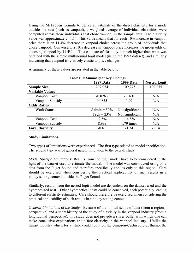
Using the McFadden formula to derive an estimate of the direct elasticity for a mode outside the nest (such as vanpool), a weighted average of individual elasticities were computed across those individuals that chose vanpool in the sample data. The elasticity value was approximately -1.14. This value means that for each 10% increase in vanpool price there is an 11.4% decrease in vanpool choice across the group of individuals that chose vanpool. Conversely, a 10% decrease in vanpool price increases the group odds of choosing vanpool by 11.4%. This estimate of elasticity is much higher than what was obtained with the simple multinomial logit model (using the 1997 dataset), and similarly indicating that vanpool is relatively elastic to price changes. A summary of these values are restated in the table below.

Table E.1: Summary of Key Findings 1997 Data 1999 Data Nested LogitSample Size 207,054 109,275 109,275 Variable Values Vanpool Cost -0.0263 -0.160 N/A Vanpool Subsidy 0.0855 1.02 N/A Odds Ratios

Admin = 50% Not significant N/A Work Status Tech = 23% Not significant N/A Vanpool Cost -2.5% -14.8% N/A Vanpool Subsidy 8.9% 1.79 times N/A Fare Elasticity -0.61 -1.34 -1.14 Study Limitations Two types of limitations were experienced. The first type related to model specification. The second type was of general nature in relation to the overall study. Model Specific Limitations: Results from the logit model have to be considered in the light of the dataset used to estimate the model. The model was constructed using only data from the Puget Sound and therefore specifically applies only to this region. Care should be exercised when considering the practical applicability of such results in a policy setting context outside the Puget Sound. Similarly, results from the nested logit model are dependent on the dataset used and the hypothesized nest. Other hypothetical nests could be conceived, each potentially leading to different elasticity estimates. Care should therefore be exercised when considering the practical applicability of such results in a policy setting context. General Limitations of the Study: Because of the limited scope of data (from a regional perspective) and a short history of the study of elasticity in the vanpool industry (from a longitudinal perspective), this study does not provide a silver bullet with which one can make conclusive explanations about fare elasticity in the vanpool industry. Unlike the transit industry which for a while could count on the Simpson-Curtin rule of thumb, the

x

limited scope of data in this study makes it difficult to provide a more generalized application of findings. However, the study provides a framework from which subsequent studies can employ diverse research and refine the methodologies towards more reliable results. These could include a wide representation of participating regions, a rich longitudinal collection of data and a significant amount of data with large and small fare changes to provide an adequate data base for analysis. Study Recommendations This study calls for a more comprehensive study that would allow for a wider scope of data from several organizations across the country. Some of the key areas to pay more attention to in future research involve the participation of multiple organizations, availability of data and interpretation of the model. Participation: First, the scope of this study was constrained by the funding resources available. To secure a large sample of data, a larger funding level will be necessary. This will help collect data from multiple locations and hopefully over a long term period. Secondly, the success of future studies will depend on the willingness of rideshare organizations and vendors to participate. In the request for data, the responses from rideshare organizations were very much limited. Without large participation, the findings from similar studies will continue to remain constrained. Thirdly, for those offering to participate, it is important that they follow up with fulfillment of the data requests. Data Availability: Related to the level of participation is the need for large, high quality and comparable data sets. First, the larger the data set, the more reliable are the findings from the analysis. However, more important is the quality of data. This includes the accuracy and representativeness of variables selected for data collection. Finally, consistency of the types of data collected between rideshare organizations is vital for both comparability of performance measures and analytical results. It is therefore imperative that the vanpool industry develop guidelines for comparable data collection. Interpretation: For a successful analysis, the model needs to recognize the multiplicity of factors influencing mode choice. Without such recognition, there is not only potential for misinterpretation of the results, but respective policy actions may be flawed. Similarly, because of the multiple factors involved, there is a need to design consistent models to provide comparable analysis and interpretation. Related to model design, it is also important to recognize the dilemma and implication of using a subsidy or a discount. While a $40 cash subsidy is materially equivalent to a $40 discount, the effects of a discount in the long run appears to diminish especially to new users who may consider the discounted fare as a regular fare, and therefore it minimizes its incentive impact.

xi

Chapter One: Introduction While several studies have been conducted to measure respective elasticities in the transit service sector, very few have been done to measure price elasticity of rideshare. Therefore, the goal of this research project was to determine the price elasticity of ridesharing modes with specific objectives of helping to assess what the effect on ridership would be if the effective price was substantially reduced. However, because of the multiple modes for providing rideshare, this research was limited to the study of vanpools. Part of the study will include the impact of subsidies on rideshare. For example, section 132(f) of the Internal Revenue Code allows most employers to provide a tax-free benefit to employees of up to $100 per month for transit and vanpool fares and up to $185 per month for parking fees. It has been hypothesized that transit and vanpool co-pay programs by employers could have a dramatic impact on transit ridership as well as other alternatives to driving alone. Given that the maximum amount an employee can apply towards the current tax benefit program is $100 per month for transit and vanpooling, it could be argued that employees who receive such a benefit from their employers could be receiving transit services at a very low cost or even for free without public subsidies and therefore, ridership potential should be significantly higher. It is uncertain whether the ranges of price changes in similar previous studies were so small that the new maximum allowable amounts of up to $100 per month co-pays were off the chart. There is no way of knowing what the impact would be on ridership since it falls outside of the range of experiences used during subsequent studies. For example, what would the impact be for large decreases in transit fares such as from $1.00 to $0.00 per trip instead of observing ridership changes for small increases such as from $1.00 per trip to $1.25 per trip? How about impacts of large increases in parking costs from free parking to $80 per month, or implementation of parking cash out? One of the objectives in this study was to include large subsidy or fare variations by companies that have made major changes in their co-payment program. The study considers the application of the Linsalata and Pham transit study methodology in the vanpool industry. The study attempted to identify gaps in current efforts to measure price elasticity of rideshare. The research reviewed literature to determine the state of the measurement practice especially as it pertains to rideshare service. Three key tasks were envisioned. First, the study reviewed literature to either refute or support the currently perceived unmet gaps, both in terms of findings and methodology. Secondly, the study collected data from both secondary and primary sources to do the analysis. Finally, based on the findings from the analysis, the study provides both policy implications and recommendations for future research needs. While data observations for the study were solicited from around the country, efforts were made to include a heavy representation from the State of Florida according to the scope of the project. This study should be applicable for determining the feasibility of rideshare pricing and would therefore primarily benefit rideshare agencies. Research into current methods of measuring price elasticity of rideshare should result in a clearer understanding of the

1

impact of pricing in the area of public transportation by Transportation Demand Management (TDM) and other transportation service provider professionals. This, in turn, should allow agencies to improve on their pricing strategies as well as increasing potential for considering alternatives to increase public transportation and thereby help reduce congestion and air pollution. The results from this study would be of particular interest to rideshare agencies, transit service providers, transportation professionals and transportation funding organizations with the potential for improving their customer service and customer base. Other organizations such as shuttle service providers, taxi companies and other transportation related companies stand to potentially benefit from the implications of the study’s results to their business. Similarly, other partial benefits are anticipated to accrue to the research community in terms of modeling and analysis.

Concept of Elasticity Elasticity is defined as the responsiveness of changes in quantity demanded due to changes in the price of the commodity in question. Therefore, rideshare elasticity measures the proportionate change in the level of ridership resulting from changes in user fares, including subsidies. Two relevant types of elasticities in this type of study include price elasticity and cross price elasticity. Price elasticity describes the change in quantity of a good or service demanded following a change in its price. For example, price elasticity of vanpool measures the percent change in vanpool ridership for every percent change in vanpool fares. Conversely, cross-price elasticity describes the change in demand for a competing (or complementary) good given a change in the price of the first good or service. An example of cross-price elasticity would be the percent change in vanpool ridership given a percent change in auto-related prices such as parking. The most common types of elasticity with respect to transportation modes are point elasticity, shrinkage ratio, midpoint arc elasticity, and constant arc elasticity. While some of the studies referenced here relied on the shrinkage ratio, the qualitative study in chapter four used the point elasticity for estimates. Two Transit Cooperative Research Program (TCRP) projects (TCRP Project H3, Policy Options to Attract Auto Users to Public Transportation, and TCRP Project H- 4A, Strategies for Influencing Choice of Urban Travel Mode) provide a good background review on this topic. Related literature on this and other different types of elasticities and the nature of the influence of price on mode choice are presented below in the literature review section.

Research Tasks There were five research tasks envisioned in this study. These included a review of current literature, further review of the state of the practice with respect to measurements or modeling, a survey/request and collection of data, analysis of data, and development of the report.

2

Research Review: This task involved a comprehensive review of past research into efforts to measure price elasticities in the service sector, especially public transportation. The review includes an examination of research conducted on other modes of transportation. This literature review identified methodologies and findings from past studies to serve as a starting point for the research. Existing literature helped avoid "reinventing the wheel" and refined specific gaps and deficiencies in the existing body of knowledge. Because of limited methodologies in rideshare analysis, the study used similar mode choice studies to develop such a process. State of the Practice of Measurement in Rideshare Industry: As indicated above, the current literature is very scanty and most transit and rideshare agencies rely on past history, intuition and/or informal observations to set their fares/price. This study identified and documented specific study methods that have been used with the goal of replicating suitable methodologies for comparative purpose. Very few quantitative studies were found to show the impact of price on rideshare ridership. These included the reports “Vanpool Pricing and Financing Guide”,2 and “Puget Sound Region Vanpool Market Assessment”.3 Surveys of Rideshare Organizations: As part of this project, the study collected primary and secondary data from a variety of sources including rideshare organizations from various parts of the country. An effort to include a significant sample from Florida was made in order to estimate the price elasticity of vanpools in Florida. Specifically, the study sought to collect data from at least 100 employers and/or organizations around the country to include, but not be limited to, 1) transit and other rideshare agencies, 2) employers and users through third party administrators such as Commuter Check, Transit Check etc, and 3) other public data sources such as the Bureau of Labor Statistics. The variables for research analysis included: (1) the levels and changes in prices or cost related factors; (2) other potentially influencing factors including but not limited to gas price, vehicle miles, parking cost, transit fares, etc; and (3) trends in ridership. Therefore, the type of data that was solicited included, 1) the amount of fare subsidies, 2) related data such as the price of gas, average vehicle miles, average parking cost, transit fares, and 3) other anecdotal information. Analyses of Findings: Findings from the literature review and data analysis were analyzed both qualitatively and quantitatively to determine the nature of price elasticity in the vanpool industry both nationally and in Florida. Final Reports: The product of this investigation is a description of current findings, including measurement tools available, data collection needs, analytic tools, level of accuracy, and results of the study. Additionally, recommendations for next steps to take are made.

2 Winters, P, and Cleland, F., Vanpool Pricing and Financing Guide, Center for Urban Transportation Research, August 2000. 3 York, B., Fabricatore, D., Prowda, B., Winters, P., and Cleland, F., Puget Sound Region Vanpool Market Assessment, WSDOT, 1999.

3

Report Organization This study is organized around five key activities, each constituting a chapter. Chapter one has provided an introductory overview of the study and related tasks. Chapter two will cover the literature reviewed before and throughout the study. Chapter three covers the quantitative analysis of the research including the methodology, application of regression analysis, use of the logit and nested logit models each with a presentation of results based on data from the Puget Sound area vanpool program. Chapter four involves a qualitative analysis ranging from tabular analysis to calculation of simple point elasticity based on data from a variety of rideshare and transit organizations. Finally, in chapter 5, several concluding observations and recommendations are made both for future studies and policy implications.

4

Chapter Two: Review of Literature and Past Case Studies The current literature is very limited especially with respect to rideshare. The types of research that have been done have typically focused on transit. Most studies on rideshare have focused on qualitative reporting or used fewer variables and therefore are limited in their scope. It is also not surprising that most transit agencies or rideshare organizations have tended to rely on rules of thumb, intuition, or less technical methods for estimating fare elasticities. However, some of the most recent studies such as the ECONorthwest and the Center for Urban Transportation Research (CUTR) study in the Puget Sound area used employer data to estimate the impact of vanpool fares and other factors to estimate mode shifts. This research study takes off from this background by reconciling with the Linsalata and Pham bus study as it applies to vanpools. It also makes advances by adding several regional observations including Florida. The goal of the study is to provide both disaggregated and aggregated measurements of fare elasticities of rideshare. The study’s quantitative analysis was done by a multiple regression and logit model approach. Similarly, a qualitative analysis was done using the point elasticity approach.

Empirical Studies A quick sample of this literature reveals that the majority of elasticity studies appear to focus on transit service. There is however, a dearth of quantitative studies related to elasticities of rideshare and vanpool in particular. Vanpool Oriented Studies As indicated before, most studies on rideshare have tended to be qualitative. For example, a survey conducted by Commuter Connections (a rideshare organization in California) focused on general patterns of sixteen agencies that responded nationwide, all had ride matching services. In terms of vanpool services, eleven were directly involved in vanpool service provision, four were not engaged and one simply provided general information. Vanpool subsidies to commuters were issued by eleven of the organizations with one organization issuing up to $400 per user in subsidies and another assisting only with initial start-up of a vanpool program. The survey also clearly revealed that the rideshare organizations had Guaranteed Ride Home Programs in place and some even offered mapping assistance, emergency ride home reimbursements, school pools and other commuter incentive programs as a means to encourage mode shifting.

Unfortunately, there are few quantitative surveys that appear to show the impact of price on rideshare ridership. Those so far available include “Vanpool Pricing and Financing

5

Guide”,4 and a report on Puget Sound Region Vanpool Market Assessment.5 One of the most recent studies on rideshare was a 1996 ECONorthwest study of the Vanpool price elasticity of the King County Department of Transportation which used employer data to develop a model for predicting mode choice.

However, this model had two major drawbacks. First, it was based on 58 observations drawn from the Commute Trip Reduction (CTR) program data of companies that had vanpool programs. This small number of observations can lead to highly unstable estimates, and the results may be biased towards vanpooling since companies with vanpooling programs in place may promote the concept more widely than what actually occurs in the general market. Secondly, there was a substantial degree of correlation between the independent variables, which made it extremely difficult (if not impossible) to isolate the impact of vanpool price differences alone. Using the ECONorthwest model, the Center for Urban transportation Research (CUTR) did a Vanpool Fare Elasticity study to predict the fraction of employees who vanpool to work. This study used the Puget Sound area 1999 CTR employer survey records on 360 employers and 229,000 commuter responses. The model was conducted as a multiple regression where the dependent variable was the logit transformation of the percentage of employees vanpooling to work, expressed as yi = log (pi / (1 - pi)). The CTR data tracks both employer programs and employee mode choice. In that study, the calculated elasticity of the fares was approximately –1.5, meaning that there is a 15% increase in demand for every 10% price reduction. Even then, the model explained only 8.2% of the variance. This means that many other factors are involved in the adoption of vanpooling as a commute mode. The identification of those factors was, however, beyond the scope of that study. CUTR was also one of the four consultants who worked on the WSDOT report about the Puget Sound region vanpool market assessment. As pointed out previously, CUTR has also done some work on an FDOT and FHA project to develop a vanpool pricing and financing guide. Transit Oriented Studies Unlike the dearth of studies on fare elasticity of rideshare, there is a multitude of elasticity studies focusing on the transit industry. Therefore, because of the close similarity between the transit and rideshare industries, the review explored a sample of these studies to help provide a broader context of fare elasticity studies in general and as a resource guide for information on methodology and analysis of rideshare elasticity in particular.

4 Winters, P, and Cleland, F., Vanpool Pricing and Financing Guide, Center for Urban Transportation Research, August, 2000. 5 York, B., Fabricatore, D., Prowda, B., Winters, P., and Cleland, F., Puget Sound Region Vanpool Market Assessment, WSDOT, 1999.

6

For example, in a study by Linsalata and Pham on “Fare Elasticity and Its Application to Forecasting Transit Demand”, the objectives of the study were to verify the Simpson-Curtin formula using updated data and modern technologies, and to provide a set of fare elasticity estimates for bus service in various cities during peak as well as off-peak hours6. The study used an advanced econometric model, the Autoregressive Integrated Moving Average (ARIMA) model, to estimate the price elasticity of bus transit. This was partially because many transit agencies continued to use this long-time industry standard which was based on an examination in the early 1960s of a number of fare increases. The formula provides a price elasticity using a shrinkage ratio of transit trips as -0.33. This implies that a 10% increase in fares would lead to a 33% decrease in transit ridership and vice versa. In the Linsalata and Pham Study, a special survey was conducted to obtain ridership data 24 months before and 24 months after each fare change for 52 transit systems. Monthly information on other factors which may influence ridership, including gasoline price, vehicle miles of service, labor strikes, etc., were also collected. The purpose was to use the model to isolate the impacts of the fare changes from those caused by other factors. On the average, a ten percent increase in bus fares would result in a four percent decrease in ridership. This shows that today's transit users react more strongly to fare changes than found by Simpson and Curtin. Transit riders in small cities were found to be more responsive to fare increases than those in large cities. The fare elasticity for bus service was -0.36 for systems in urbanized areas of 1 million or more population. In urbanized areas with less than 1 million people, the elasticity was -0.43. However, other works have similarly shown that the Simpson-Curtin rule is not a constant, and that there are, in fact, a wide range of price elasticities. For example, the TRIPS model for home-based-work trips, calibrated for Los Angeles conditions, suggested an elasticity of about -0.08.7 In another study, Goodwin (1992) found average bus fare elasticity from 50 studies as -0.41. Another related study by Richard Voith, "The Long-Run Elasticity of Demand for Commuter Rail Transportation,"8 aimed at analyzing rail transit ridership in the Philadelphia area to determine how users respond to changes in transit price, service levels (e.g., train frequency), and alternative transportation options (e.g., cars). The results indicated that transit riders were twice as responsive to changes in these factors in the long run compared to the short run. Attempts to balance transit budgets by increasing fares and reducing service quality were thus likely to result in higher subsidies and deficits. The paper measured the long-run change in rail transit ridership resulting from changes in price and service (elasticity). The study used data from the Southeastern Pennsylvania Transportation Authority (SEPTA) which operates a commuter rail system in the Philadelphia metropolitan area. Data included ridership, fares, and service

6 Linsalata, J. and Pham, L, Fare Elasticity and Its Application to Forecasting Transit Demand, American Public Transit Association, 1991. 7 Stephen Andrle, Coordinated Intermodal Transportation Pricing and Funding Strategies- Research Results Digest- Number 14- October 1997. 8 Journal of Urban Economics 30 (1991), pp. 360-72.

7

attributes for 129 of 165 stations in the SEPTA system for 12 separate points in time from 1978 to 1986. Using Maximum Likelihood Estimation, the author estimated that "the long-run response to changes in prices and service attributes are 2.6 times larger than short-run responses." The average lag is about one year. The long run estimates of elasticity were large. "In the long run, demand is strikingly elastic with respect to own price (-1.59), the variable cost of an auto trip (2.69), and the fixed cost of auto ownership (1.13)." From a Policy perspective, the study found that ridership is more than twice as elastic in the long run as in the short run. Ridership on SEPTA, which was price inelastic in the short run, was price elastic in the long run, usually an expected result. The characteristics of service such as frequency and speed of trains, and alternative transportation prices, have significant effects on ridership, which are substantially larger in the long run than in the short run. It can be argued that the long-term elasticities are higher than the short-term effects because travelers in the long-run can move or buy a car, whereas they may initially be more captive to the bus in the short-term. The findings suggested that reductions in public transportation subsidies that result in higher fares and lower service quality may produce higher subsidy costs per rider than would be the case with higher total subsidy. Public Subsidy As evident from the preceding study, some alternative analyses have focused on public subsidy effect. For example, in the “Zero Elasticity Rule for Pricing a Government Service”, the study investigated the properties of the "zero-elasticity" pricing rule in which the agency sets an initial price, observes the resulting usage of the service, assumes that demand is totally price-inelastic and replaces the initial-price with one calculated to solve the budgetary problem, and then observes the usage that actually occurs and reapplies the zero-elasticity assumption. The study argued that government agencies often offer services or subsidies for which the demand is unknown. It focused on the problem faced by such an agency when it must select a price-subsidy level so as to meet a budget constraint. The study presented analytical results on the dynamics of iterated use of the rule, particularly its convergence to a price solving the budgetary problem using a case study of local transit pricing.

TCRP Project H-6 Synthesis: A Comprehensive Review Two of the good resources for literature review on elasticity studies, particularly with respect to transit and rideshare modes are in the TCRP project H-6, “Transit Fare Pricing Strategy in Regional Intermodal Systems” and the TCRP 95 series on “Traveler Response to Transportation System Changes.” This review summary pertains to the TCRP Project H-6 synthesis. It should be noted that the TCRP Project H-6 study did not focus on the identification or development of elasticity measures. It simply provided a synthesis of fare elasticity related literature. A sample of pertinent topics include; 1) price elasticity for transit, 2) cross price elasticity for auto use with respect to transit price, and 3) cross price elasticities of transit use with respect to auto price. A brief summary of each is presented here.

8

Price Elasticities for Transit According to the TCRP Project H-6 synthesis, one of the studies focusing on price elasticity of transit is Lago, et al. (1992). Thus, in the survey of transit price elasticities, Lago presented results from more than 60 studies of elasticities and cross-elasticities. The study disaggregated the effects of price among a variety of conditions and groups. The project synthesis also provided five major types of sources of transit elasticities:

• Time series analysis of the agency's historical ridership data; this often includes a regression analysis to isolate the effects of fare changes from other factors, such as service changes, employment, or fuel prices;

• Before-after ("shrinkage") analysis for a particular fare change; • Use of a demand function, often based on the results of stated preference surveys

(i.e., asking how people would respond to various fare options and changes, or alternatively asking them to "trade off" fare changes with level of service changes);

• Review of industry experience, particularly for agencies of similar size and with similar characteristics; and

• Use of professional judgment in adjusting figures derived from above sources. All these studies provided a good glimpse of different methodologies for calculating price elasticity of transit depending on availability of data and objectives for analysis. Cross-Price Elasticities of Auto Use with Respect to Transit Price The TCRP Project H-6 synthesis also highlighted a number of studies that have focused on cross elasticity of auto use with respect to transit price. One of the extreme perspectives is that of Domencich and Kraft who concluded in their 1970 study that it would be necessary for transit agencies to pay people to lure them from their cars. One of the possible explanations for such perspectives was provided by Lee (1992) who suggested that the issue is quite complex but that the reality is the cost of auto travel is such a small part of most household incomes that transit cannot be made sufficiently attractive just by lowering its price. Thus, improved transit service qualities are more important than lower fares in attracting auto users to transit, although it is clearly difficult for transit to provide even a near substitute for the qualities of most auto trips. The synthesis also stressed the point that demand modeling efforts typically assume shifts of trips lost from one mode (e.g., transit) to the other available mode(s), but these are limited in that they typically assume that no trips are foregone altogether. Therefore, the analysis of fare change effects (either projected or after-the-fact) focuses simply on the change in transit trips, without regard to the "redistribution" of the lost trips. One study that the synthesis finds to have estimated the effect of a fare increase on auto usage was by the Massachusetts Bay Transportation Authority (MBTA). The MBTA examined the environmental effects of a 1991 fare increase that decreased weekday system wide

9

ridership by nearly 6%. In the Draft Environmental Impact Report on the 1991 Fare Increase, the MBTA estimated that the total increase in regional Vehicle Miles Traveled (VMT) was 110,685 per weekday (assuming that all lost transit trips shifted to private automobile), or 0.15% of the regional total of 73 million VMT. Cross-Price Elasticities of Transit Use with Respect to Auto Price The synthesis stressed the point that demand modeling efforts typically assume shifts of trips lost from one mode (e.g., transit) to the other available mode(s), but these are limited in that they typically assume that no trips are foregone altogether. Therefore, the analysis of fare change effects (either projected or after-the-fact) focuses simply on the change in transit trips, without regard to the "redistribution" of the lost trips. For example, with respect to cross-price elasticity of transit and the automobile, the TCRP Project H-6 synthesis revealed that while numerous studies have shown that increasing the costs of driving has reduced the share of drive alone commuting, the effects on transit use are less clearly understood. The synthesis argued that raising the price of auto travel will lead some motorists to shift to transit, but the greatest effect of a price increase (assuming that the price change is noticeable at all) would likely be in the growth of ridesharing or simply fewer trips. However, it pointed out that since the relative proportions of trips taken by transit versus auto is so lopsided in most areas, a small percentage of auto trips lost to transit would mean a much larger percentage of transit trips gained from auto. For example, Lago reported that the mean cross-elasticity of transit demand with respect to total automobile costs was +0.85.) It has been determined that the availability of free parking has the biggest impact on mode choice, while changing parking prices will have significant, but lesser, effects. Willson (1992) used data from a 1986 mode-choice survey of downtown Los Angeles office workers in a logit model for mode choice and parking demand and estimated that elimination of free parking would reduce SOV share from 72% to 41%, increase carpool share from 13% to 28%, and double the transit share from 15% to 31% of employee travel. The computed cross elasticity for transit was +0.35. The synthesis also observed that the few other studies that have sought to estimate the effects of fare changes on other modes have found the cross-elasticities of auto use with respect to transit prices to be quite low. For example, a study by Lago et al.(1992) found the mean cross-elasticity of auto demand with respect to bus fares to be +0.09 -+0.07 (eight cases), and +0.08 -+0.03 (three cases) with respect to rail fares. These results suggest that the cross elasticities related to transit fares are significantly lower than the straight fare elasticities. Kain (1994) looked at the relationship between congestion pricing (or comparable increases in driving costs) and mode choice in some detail. Kain believed that previous analyses and discussions underestimated the shift to transit that would take place with the implementation of congestion pricing and overestimated the level of tolls that would be required to achieve desired congestion levels." (Kain, p. 531). Implementing congestion pricing would make transit and carpooling more attractive. First, solo driving would become more expensive in relation to high-occupancy modes. Second, reducing roadway

10

congestion will improve trip times and reliability for these alternative modes. (Even rail trips with exclusive rights of way would benefit from improvements in road-based passenger access.) Third, as Shoup (1994) also points out, congestion pricing would increase the number of potential carpool matches as more commuters seek alternative modes. Finally, if transit demand increases sufficiently, transit operators might respond by expanding service frequencies and route coverage-- thereby further increasing transit demand. Similarly, the synthesis argued that the relationship between transit and carpooling is not well understood. For example, it points out Shoup’s (1994) hypothesis that cashing out parking would "reshuffle cars and commuters in some surprising ways." Not only would carpooling increase, but this shift could increase the number of people commuting to work in automobiles, especially if former solo drivers recruit transit passengers for their new carpools. Moreover, if transit passengers shift to carpools, cashing out parking could reduce peak-hour transit ridership. Another study reviewed in the synthesis included DeCorla-Souza and Gupta (1989) who explored the effect of auto pricing and transit policies working together to shift travel demand to higher occupancy transportation. In their analysis, they used computerized travel models to forecast mode choice under several alternative policies. For example, under a transit-preferential strategy, which included high-level peak-period transit supply and pricing policies to encourage transit (reduced fares) and discourage auto use (tolls and parking charges), they forecasted a 35% contraction in peak-period SOV work travel in the year 2010 compared to a traditional context. They forecasted that policies focusing only on ride-sharing would be less effective and that a combination transit/ride-share strategy would divert more travelers from SOV, though transit would capture fewer of these than under a transit-only focused strategy. It is clear that there are very limited quantitative elasticity studies from these studies with respect to rideshare including vanpool. It is also obvious from these studies that the transit industry has received a large share of the quantitative elasticity studies since the Simpson-Curtin Rule (elasticity of -0.33). Most of these studies have provided a wealth of information, methodologies, findings and issues. Given the strength of these studies and the similarity between transit and the rideshare industry, it is assumed that these studies and their respective methodologies may be used to enhance similar studies in the rideshare industry.

11

Chapter Three: Quantitative Analysis This research project aimed at determining the price elasticity of ridesharing with specific objectives of helping to assess what the effect on ridership would be if the effective price paid by the traveler was substantially reduced (i.e., increase in employer co-pay) or increased (i.e., decrease in employer co-pay). Due to the multiple modes for providing rideshare, this research was limited to the study of vanpools.

Research Design and Methodology In this section, we review the process for identifying pertinent variables and collecting data and discuss the methodology for analyzing data. Research Design The study included the review of literature, request for data through a national listserv, and data analysis at both quantitative and qualitative levels. Initially, the Linsalata model from the transit industry was identified as the ideal framework for replication in this vanpool study. However, because of the difficulties of collecting data, the model was readjusted to take these limitations into account. Review of Literature: The review of literature focused on four key areas; fare elasticity studies in general, fare elasticity with respect to vanpools, fare elasticity with respect to transit (as a source for modeling) and respective analytical models. The sources for literature review included TRIS Search, TRB 2003 Annual Meeting CD-ROM, Google Search, Center for Urban Transportation Research (CUTR’s) CRIC Library and a collection of literature previously compiled on elasticities by the TCRP Project H-6. Request for Data: The request for data was sent out through a national listserv requesting any organizations with data on rideshare programs to provide it. The request itemized the study’s key areas of interest for data. Because of the low responses, it was assumed that some agencies may not be willing to sort and isolate requested information. Therefore, a further request was sent to non respondents requesting them to send in any type of data they had without having to sort it out. This also resulted in limited responses especially for Florida organizations for which this study intended to constitute a large portion of the sample (since the study was interested in comparing Florida vanpool experiences relative to other select organizations around the country). Further e-mails and phone calls were made to solicit more participation from Florida organizations which resulted in responses with varying degrees of data information. These ranged from those with simple fare schedules to those with a variety of variables over a period of several years. Data Analysis: The analysis of data took two forms. First was the quantitative analysis which required a huge data set and applied regression and Logit models. Because of limited sources for data, the Puget Sound area data set was used for this analysis. With a

12

data set of 262,354 employee records for 1997 and 273,234 employee records for 1999 the data was sorted to obtain useful data with which the regression analysis could be done.9 Consequently, because of the type of data available and budgetary constraints, the 1997 data was used with a further analysis using the 1999 data for comparison. The second type of data analysis focused on qualitative analysis. This ranged from tabular representation to simple elasticity analysis. For some of the organizations that had data with previous changes in fares, a simple elasticity was done using the before and after data. The goal was to show the responsiveness of ridership given the change in the fare (unlike the above quantitative analysis, this method assumed other factors constant). 10 For other organizations without fare changes or limited data information, a tabular representation was used to simply highlight trends (and possible correlations) without any indications of potential causes. Methodology A comprehensive review of current practices and techniques for the estimation led to varied procedures for calculating the price elasticity of a particular mode. The study identified and documented specific study methods that have been used with the goal of replicating suitable methodologies for comparative purposes. The findings from these studies led to the development of a set of variables that are believed to be key determinants of a price elasticity of vanpools. The Study Hypothesis: This study initially hypothesized certain factors that would influence ridership along with changes in the fare structure based on the Linsalata and Pham study. This hypothetical structure of the model was initially defined for use to solicit data. However, while the eventual model that was used in this study was modified to account for data limitations, the original hypothetical structure is presented here for purpose of context. The hypothesized model structure was therefore to be as follows:11: Rt = FCt +ACt +MCt +SLt +TROt + ∈t

Where:

• Rt= ridership • FCt = total costs of traveling by vanpool, transit and vanpool (fares and subsidy)

9 Estimation of elasticities from this data did not include tracking changes in demand based on a change in price. In other words, even though we looked at two time periods, we estimated elasticity in sort of a cross sectional analysis that assessed propensity to vanpool at different fare levels and with or without the presence of subsidies. 10 For other influencing factors, see also Lee, Lee & Park at http://www.koti.re.kr/project/coop.nsf/1F4EDE0921545E2949256DF60010D2AE/$file/urban.pdf and Pratt http://gulliver.trb.org/publications/tcrp/tcrp_webdoc_12.pdf

13

• ACt = total costs of traveling by an alternative mode • MCt = travel market characteristics including city size and demographics • SLt = level of service and accessibility supplied by the vanpool program. • It = intervening factor represented by Trip Reduction Ordinance factors • ∈t = random error

Where proxies for variables used include:

• Cost- daily per mile ride or price/mile ratio. • Alternative/Auto Cost- fuel costs and parking costs • Subsidy- looking for substantial changes to determine elasticity values (agencies

asked to submit a before and after value for a subsidy in a time period of between two years).

• Service Level- revenue service hours and travel time are considered (take distance and divide by time to determine a value for ‘speed”, since vanpools are always revenue generating). Higher speeds of the vanpool will bring the service levels in terms of speed closer to automobile speeds.

• Market Size- employment levels-Vanpools are strictly for employment in the context of this study, thus there will be more accuracy as opposed to transit.

• Other Intervening Factors - Trip Reduction Ordinances/Commuter Trip Reduction, where the presence of TROs is assigned a 1, and where a TRO is not present is assigned a 0.

• Error Term- Other factors that may contribute to ridership that may not be captured within/by the explanatory variables in the model that affect the elasticity of vanpools.

Explaining Hypothesized Variables: Each of these variables is in turn elaborated as follows: 1. Ridership Variable The ridership variable Rt is the dependent variable to be estimated by the independent variables below. It is based on the number of participants in a respective vanpool program (as a whole). The estimation determines the long term and short term impact of a large cost change on ridership along with other variables. In a study by Dargay and Hanly entitled, “Bus Fare Elasticities”, the authors found linkages between income, car travel, and bus usage. It suggested that the price substitution between both modes of travel tended to be more elastic in the long-run (measured over a seven year period- ample time for commuter adjustments). 2. Fare Cost Variable Fare cost variable FCt at time t would constitute a natural logarithm of cost per mile calculated as follows:

• Collect monthly data on fares paid by vanpool commuters less the subsidy (where applicable and provided)

• The monthly fare data is converted into daily rate (monthly rate divided by 22 days).

14

Daily rates were to be converted into daily cost per mile to provide a basis for comparison (daily rate divided by daily distance). The cost variable was the gross cost to the vanpool commuter for travel from the assigned pick us destination to the workplace. It was represented as a daily per mile or price/mile ratio, both logged to remove the correlation between price/fare and distance. In a survey taken by RIDES in their 1999 Vanpool Driver Survey, they found that the average one way commuting distance for vanpools was 49.2 miles and the vanpool fare for passengers was $110.00. This yields a daily price per mile ratio of $0.05 per mile.12

The subsidy represents the employer’s13 contribution to provide a strong incentive for employees to consider vanpooling as an alternative to driving. The model will estimate how a large change in a subsidy level would affect vanpool ridership by determining elasticity values based on data from selected agencies before and after changes in the subsidy level (the study used a dummy variable for subsidy). Thus, the subsidy essentially represents the difference between the net and gross cost to the vanpool rider for vanpooling to work on a monthly basis. The subsidy level is a key determinant in the level of ridership changes that will occur with a change in the vanpool fare, as it is where the vanpooler faces a change in the net cost of vanpooling. 3. Alternative/Competing Mode Cost Variable Alternative mode cost variable ACt would be based on the cost of an automobile since the drive alone/automobile mode is the most significant competitor to vanpools. The calculation includes fuel prices in the respective area and the relative parking rates added together as a proxy to total cost of driving alone. The parking rates allow for the inclusion of firms that offer parking cash-out to employees represented in the model as an increasing cost of parking. This is due to the opportunity cost to the commuter of forgoing the cash-out should they still decide to drive to work. Parking cash-out programs essentially encourage the use of other modes of transportation, giving the commuter the opportunity to face a gain in income for not parking. The cost of fuel per gallon can be drawn from the areas surveyed based on regional and local rates. 4. Travel Market Characteristics Variable The market characteristics variable MCt is based on employment numbers in the area to determine the market size variable that determines vanpool demand in the area. Thus the survey includes collection of data about the employment levels of the area to be able to account for this within the model framework. The market size is a key determinant in the level of ridership in terms of vanpooling to a distinct work area. For instance, employment levels are a major factor in the volume of ridership. Market size is usually determined by demographic data such as population, income, age and employment that determines income. In the 1991 APTA Study,

12 See www.rides.org/main/vanpoolstudy99.pdf 13 The subsidy could also include subsidies from other entities, such as rideshare organization, other government agency, TMA, city, etc.

15

employment elasticities were estimates ranging from 0.50 to 0.70, implying that as employment decreases, so does ridership. 5. Intervening Variable The last variable It, is the intervening factor that simply can be a dummy response variable set before agency participants as a 1, implying the presence of a Trip Reduction Ordinance or a 0 implying the absence of a TRO. TRO’s primary goal is to reduce automobile traffic and/or congestion and increase transit or carpool use.

The intervention variable looks at whether there is a TRO (Trip Reduction Ordinance) in legislation in the respective work area. TROs that aim at reducing automobile traffic and congestion and increase transit use and alternative modes through employer-based programs would certainly increase the possibility of a vanpool subsidy program being in place. The 1991 APTA study notes that there are two characteristics of the intervention that must be specified, “a priori”, namely the starting point and the general shape or expected nature of the intervention. Consequently, where there is a TRO, the dummy variable is assigned a 1.

Puget Sound Case Study Based on the identification of these variables, a request for data was made to rideshare organizations and vanpool agencies across the country. Further effort was made to obtain more data from Florida organizations. The agencies were sent electronically a formal letter describing the scope of the study and a form that outlined in detail the raw data for the elasticity model. The agencies were further asked to note any changes in the cost to riders (increase in fare or change in subsidy where known). The agencies contacted were in particular asked to provide any additional comments that would lend insight into their respective operations and sites. Unfortunately, there was a very low response from rideshare organizations. As a result, the study was only able to perform a quantitative analysis using the Puget Sound data. Therefore, most of the other data was used to perform qualitative analysis in a later section of the report. Objective of the Analysis Using Puget Sound Data Because of the rich data, along with associated limitations, the specification for variables was adjusted to include a utility approach. Therefore, this analysis considers the use of logistic regression modeling techniques to investigate the choice of vanpool services and the effects of subsidy programs and price on vanpool demand. Using employer and employee data from the 199714 Commute Trip Reduction (CTR) program surveys of the state of Washington, a conditional discrete choice model is built to analyze the choice of vanpool services with respect to competing means of transportation as a function of various socio-economic characteristics. 14 The 1977 data had the largest sample of useful data after cleaning.

16

The purpose of this model was to estimate changes in demand that would occur as a result of changes in vanpool prices. It also addresses some of the issues and shortcomings of similar previous models, specifically:15

The model is based on mode choice, accounting for competing modes of

transportation It includes socio-economic predictors, in particular the employee job descriptions

as reported in the employee survey It assess the impact of subsidy on the choice of vanpool services It provides a new estimate of elasticity of vanpool choice with respect to its price

The model relies on theoretical assumptions that have their underpinnings in microeconomic theory of consumer choice and transportation demand analysis. However, it is beyond the scope of this study to provide a formal treatment of the theoretical model of mode choice and its application in transportation demand analysis16. This analysis is broken into two segments. The first segment uses the 1997 data to provide a basic analysis of variables, their respective impacts on mode choice and elasticity with respect to price change/subsidy. The second segment does the same analysis using the 1999 data but uses actual subsidy amounts instead of dummy variables. It also uses employment dummy variables instead of jobs dummy variables. Data Analysis Using 1997 Data Set In Section 1.1, the sample survey dataset is analyzed and the appropriate set of variables to estimate the model is described. In Section 1.2, the approach to model building is outlined and the model is estimated and checked against violations of assumptions; after the model is validated, parameter inference is conducted. In Section 1.3, conclusions and caveats are considered. DATA DESCRIPTION The data used in the model are derived from the CTR survey, and constitute the “observational data” portion of the dataset. The cost variables of each mode of transportation taken into consideration were constructed and linked to the home/work round trip distance traveled by each respondent; they constitute the “designed or derived data” portion of the overall dataset.

15 See a previous study by CUTR “Vanpool Pricing and Financing Guide” at http://www.cutr.usf.edu/tdm/pdf/Vanpool_values.pdf 16 For a formal treatment of discrete choice models in transportation demand analysis see McFadden, D. (1981) “Econometric Models of Probabilistic Choice,” in C.F. Manski and D. McFadden (eds.), Structural Analysis of Discrete Data with Econometrics Applications, 198-272, Cambridge: MIT Press.

17

Observational Data The dataset used to run this portion of the model is derived from two separate surveys from the 1997 Commute Trip Reduction (CTR) program. The CTR data is part of a major effort conducted in the state of Washington to track both employer programs and employee mode choice. First is the employer survey dataset, which provided information on mode specific subsidy programs. From this dataset it was possible to extract both quantitative and qualitative information on subsidies for vanpool, carpool, and transit programs respectively Next is the employee survey, which is a survey of revealed preferences via actual travel behavior in response to real costs, options, and other factors. Commuters were asked what their choice of transportation was in the week prior to the day they were surveyed. This characteristic, together with similar other sets of questions present in the survey, make the dataset sufficiently fit to discrete choice analysis. From the CTR employee survey, the following information was extracted for consideration in the model building process.17 This included mode choice, work status and distance. 1. Mode Choice: The employees were asked what means of transportation they used the week prior to the survey day. This constitutes the mode choice set, which is comprised of the following means of transportation:

Drive Alone Carpool Vanpool Bus/Transit Bicycle Motorcycle Walk Telecommuting Other

In order to concentrate on vanpool choice, the dataset was resized to consider only a mode choice subset including the following modes:

Drive Alone Carpool Vanpool Bus/Transit

This restriction does not imply a relevant loss of information. The other modes were not considered to be close substitutes for vanpools. 17 For elements of a sample of the survey questions, see Appendix 1.

18

2. Work Status: The employees were asked to report their occupation. The question was designed in a somewhat broad format, allowing assessing the industry of occupation and generic title. Nonetheless, a distinction between lower, middle, and high skill position could still be obtained. The objective was to analyze and assess if a particular type of occupation has influence on mode choice. 3. Distance: The employees were asked to report the distance from home to work, and to specify if it was an estimate or an accurate measurement. The quality of response supports evidence of a reliable and accurate measurement of the reported distance. The reported distance was used to construct the mode specific cost variables, as described later below. Constructed Data Since the cost of using each mode of transportation was not reported in the employee survey, each of the cost variables were constructed based on a set of assumptions. These included drive alone cost, carpool cost, vanpool cost, transit cost and mode subsidy. The cost components of each mode are described below along with dummy variables created for work status. 1. Drive Alone Cost (DA_COST): The costs components and estimates used to construct this variable were derived directly from the American Automobile Association (AAA). According to AAA, the average operating cost of an automobile was about 13.4 cents per mile in 2001. Operating costs include gas, oil, maintenance, and tires. Using this estimate (adjusted to reflect the cost of living as of 1997), and the employee reported distance, this variable was created as follows: DA_COST = DIST * COST + PARKING Where:

DIST = distance; reported daily round trip distance as per employee survey

COST = daily average operating cost; AAA 2003 estimates rolled back to the cost of living as of 1997 using Consumer Price Index for 1997 = $0.1145

PARKING = Average reported daily parking cost as per employee survey, across all reported counties = $1.53

Assuming an average of 22 working days per month, the drive alone cost (DA_COST) variable was translated into a daily cost.

2. Carpool Cost (CP_COST): To account for the cost of carpooling, the general guidelines of commuter reduction programs were considered. For example, according to the Spokane County Commute Trip Reduction program,18 the guidelines for charging

18 See http://www.transmatch.org/tm/cpoolqna.php

19

carpool passengers suggest using the auto cost estimates as derived above, and divide it by the number of passengers carpooling. Using the reported vehicle occupancy in the employee survey, this variable was created as follows: CP_COST = (DA_ COST/ SURVEY REPORTED OCCUPANCY) = DIST * COST + PARKING / SURVEY REPORTED OCCUPANCY

Where:

DIST = distance; reported daily round trip distance as per employee survey

COST = daily average operating cost; AAA 2003 estimates adjusted using CPI for 1997 = $0.1145

PARKING = Average reported daily parking cost as per employee survey, across all reported counties = $1.53

Assuming an average of 22 working days per month, the carpool cost variable was translated into a daily cost. 3. Vanpool Cost: This variable was constructed using information from both the employer and employee surveys. By using the reported response identification code number, each survey respondent in the employee survey was matched to each respective firm in the employer survey. Using this matching procedure, the fare schedule of each vanpool company serving the county within which the employer is located was used. The fare schedules are based on distance and are published as a monthly cost. Using the employee reported distance the vanpool cost variable was constructed. Assuming an average of 22 working days per month, the vanpool cost variable was translated into a daily cost. 4. Transit Cost: Using the employer/employee survey matching procedure, transit costs were derived using published fare schedules, using the county within which the employer is located. 5. Mode Subsidy: Using the employer/employee survey matching procedure, it was possible to determine which firms offer a carpool, vanpool, or transit subsidy. Three additional dummy variables were created to indicate the presence or absence of mode subsidies. They are coded as follows:

Table 3.0 Subsidy Dummy Variables

Dummy Job TypeVP_SUB Vanpool Subsidy (1 if yes, 0 otherwise)CP_SUB Carpool Subsidy (1 if yes, 0 otherwise)TR_SUB Transit Subsidy ( 1 if yes, 0 otherwise)

6. Work Status: Using question number eight of the employee survey, a set of six dummy variables was created to express the work status of the respondents. The objective was to

20

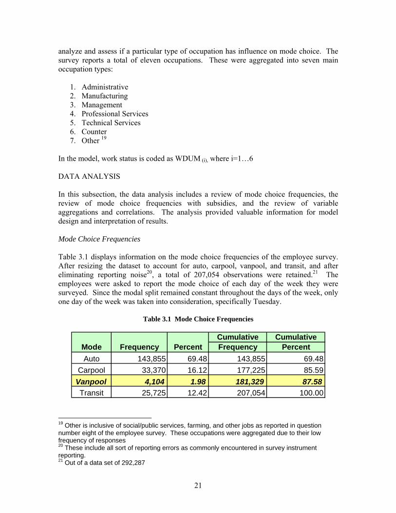
analyze and assess if a particular type of occupation has influence on mode choice. The survey reports a total of eleven occupations. These were aggregated into seven main occupation types:

1. Administrative 2. Manufacturing 3. Management 4. Professional Services 5. Technical Services 6. Counter 7. Other 19

In the model, work status is coded as WDUM (i), where i=1…6 DATA ANALYSIS In this subsection, the data analysis includes a review of mode choice frequencies, the review of mode choice frequencies with subsidies, and the review of variable aggregations and correlations. The analysis provided valuable information for model design and interpretation of results. Mode Choice Frequencies Table 3.1 displays information on the mode choice frequencies of the employee survey. After resizing the dataset to account for auto, carpool, vanpool, and transit, and after eliminating reporting noise20, a total of 207,054 observations were retained.21 The employees were asked to report the mode choice of each day of the week they were surveyed. Since the modal split remained constant throughout the days of the week, only one day of the week was taken into consideration, specifically Tuesday.

Table 3.1 Mode Choice Frequencies

Cumulative CumulativeMode Frequency Percent Frequency PercentAuto 143,855 69.48 143,855 69.48

Carpool 33,370 16.12 177,225 85.59Vanpool 4,104 1.98 181,329 87.58Transit 25,725 12.42 207,054 100.00

19 Other is inclusive of social/public services, farming, and other jobs as reported in question number eight of the employee survey. These occupations were aggregated due to their low frequency of responses 20 These include all sort of reporting errors as commonly encountered in survey instrument reporting. 21 Out of a data set of 292,287

21

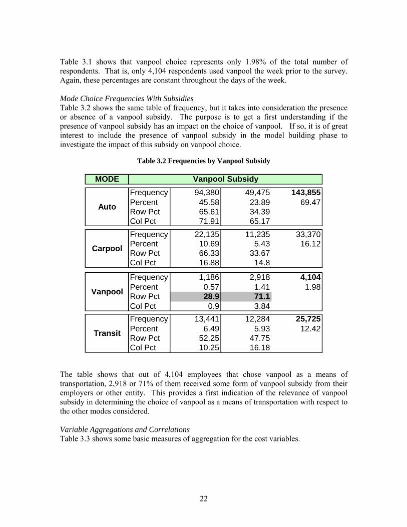
Table 3.1 shows that vanpool choice represents only 1.98% of the total number of respondents. That is, only 4,104 respondents used vanpool the week prior to the survey. Again, these percentages are constant throughout the days of the week. Mode Choice Frequencies With Subsidies Table 3.2 shows the same table of frequency, but it takes into consideration the presence or absence of a vanpool subsidy. The purpose is to get a first understanding if the presence of vanpool subsidy has an impact on the choice of vanpool. If so, it is of great interest to include the presence of vanpool subsidy in the model building phase to investigate the impact of this subsidy on vanpool choice.

Table 3.2 Frequencies by Vanpool Subsidy

MODE

Frequency 94,380 49,475 143,855Percent 45.58 23.89 69.47Row Pct 65.61 34.39Col Pct 71.91 65.17Frequency 22,135 11,235 33,370Percent 10.69 5.43 16.12Row Pct 66.33 33.67Col Pct 16.88 14.8

Frequency 1,186 2,918 4,104Percent 0.57 1.41 1.98Row Pct 28.9 71.1Col Pct 0.9 3.84Frequency 13,441 12,284 25,725Percent 6.49 5.93 12.42Row Pct 52.25 47.75Col Pct 10.25 16.18

Vanpool Subsidy

Transit

Auto

Carpool

Vanpool

The table shows that out of 4,104 employees that chose vanpool as a means of transportation, 2,918 or 71% of them received some form of vanpool subsidy from their employers or other entity. This provides a first indication of the relevance of vanpool subsidy in determining the choice of vanpool as a means of transportation with respect to the other modes considered. Variable Aggregations and Correlations Table 3.3 shows some basic measures of aggregation for the cost variables.

22

Table 3.3: Cost Variable Aggregations

Variable Mean Std Dev Minimum Maximum

Drive Alone 4.66081 2.26733 1.75900 14.12500

Carpool 4.18243 2.34045 0.25129 7.0625

Vanpool 2.22900 1.07610 0.84000 8.22000

Transit 2.06252 0.56266 1.00000 2.50000 The daily cost of vanpooling ranges from $0.84 to a maximum of $8.22, with a daily average of $2.22; carpooling costs range from $0.25 to a maximum of $7. These costs do not include any subsidy the employees could receive; subsidies are treated as a separate categorical variable in the model building phase. Table 3.4 displays the relative Pearson correlation coefficients.

Table 3.4 Pearson Correlation Coefficients

Drive Alone Carpool Vanpool Transit Distance

Drive Alone 1.00000 0.76146 0.58153 0.10936 1.00000

Carpool 0.76146 1.00000 0.48421 0.10101 0.76146

Vanpool 0.58153 0.48421 1.00000 0.17392 0.58153

Transit 0.10936 0.10101 0.17392 1.00000 0.10396

Distance 1.00000 0.76146 0.58153 0.10396 1.00000

Pearson Correlation CoefficientsMode Costs

The correlation coefficients in Table 3.4 indicate the presence of a linear relationship between some of the cost variables, such as drive alone and carpool. This is due to the way the two variables were constructed. This correlation could resurface when the model is estimated in terms multicollinearity. Consequently, multicollinearity tests were conducted accordingly in the model building section. THE MODEL The objective was to build a model that could ultimately account for a set of relevant factors affecting the choice of vanpool as a mode of transportation with respect to the other modes being considered. The proposed model considers the presence of vanpool subsidy as a qualitative variable, set up as a dummy with a value of one indicating the presence of the subsidy and with

23

zero indicating its absence. The model estimates the effects of a subsidy on the probability of choosing vanpool with respect to auto. The intent is to estimate the impact of vanpool price and subsidy on vanpool choice by implementing a discrete choice modeling approach in the form of a multinomial logit model. This model is best suited to analyze the relationship between a discrete dependent variable representing the choice set that an individual faces (the modes of transportation herein considered and a set of continuous and/or categorical predictors). It is assumed that the individual chooses that mode that provides the highest level of satisfaction (i.e. utility), given the set of individual and mode specific characteristics. Below are the details of the model:

Dependent variable: Mode (drive alone, carpool, vanpool, transit)

Independent or explanatory variables: o Choice specific:

Mode costs (for each of drive alone, carpool, vanpool, and transit) Subsidy (for each of carpool, vanpool, and transit)

• In discrete values with each represented by a two-level dummy.

o Individual specific: Work status: ( in discrete values: a six-level dummy, as described

above) The model was estimated by means of the maximum likelihood using the SAS statistical package. The Regression Model However, before estimating the model and making any inferences, a regular regression model was run with specific options to investigate the presence of multicollinearity (a situation where it is impossible to attribute changes in the dependent variable to a specific independent variable). The variance inflation factor (VIF) was used as an indicator of the presence of multicollinearity. Given that the VIF ranged between 1.5 and 2.7 (well below the usual threshold of 7), it was concluded that the model does not suffer from any relevant multicollinearity. Therefore all the explanatory variables were retained. The model was also validated by randomly splitting in half the original dataset into two sub-datasets. The first sub-dataset was used to estimate the model. The model was checked against the second dataset for predictive power. The pseudo R2 was used as a measure of predictive power. The model performed satisfactorily as the R2 moved from 0.2055 to 0.2066. Finally, the datasets were re-merged together and the final model estimated. Table 3.5 shows the test statistic for assessing the overall adequacy of the model (null hypothesis: all coefficients are equal to zero). The test statistic is given by the chi-square value of the

24

log-likelihood ratio. At an observed p-value less than 0.0001 it can be concluded that the model is adequate for predicting mode choice.

Table 3.5 Test Statistics

Model Fit StatisticsScore Test for the Proportional Odds Assumption

ChiChi--Square DF Pr > Square DF Pr > ChiSqChiSq273580.260 26 <.0001273580.260 26 <.0001

InterceptIntercept and

Criterion Only Covariates

AIC 352456.16 315051.50SC 352486.78 315214.81-2 Log L 352450.16 315019.50

R-Square 0.1706 MaxMax--rescaled Rrescaled R--Square 0.2060Square 0.2060

Testing Global Null Hypothesis: BETA=0

Test Chi-Square DF Pr > ChiSq

Likelihood Ratio 37430.6584 13 <.0001Likelihood Ratio 37430.6584 13 <.0001Score 52049.4192 13 <.0001Wald 26628.0222 13 <.0001

By looking at the adjusted pseudo R2 value, the model explains about 20% of the sample variation in the dependent value (mode choice), after adjusting for the sample size and number of independent variables in the model. A similar previous model explained 8% of the variation.22 However, other factors can potentially intervene in the choice of the vanpool as a means of transportation that this model does not account for, which are outside the focus of this analysis. Looking at the parameter estimates in Table 3.5, the first section of the table shows the global tests for the effects of each variable on the outcome variable (mode choice), controlling for the other variables in the model. The reported chi-square statistics tests the null hypothesis that the explanatory variables have no effect on the outcome variable. By looking at the observed p-values (at α=.5), it appears that all of the explanatory variables are significantly different from zero. Parameter Inference The model was estimated using drive alone as the base mode. That is, when interpreting the parameters, the comparison is between the effects of a given parameter on the choice of vanpool, carpool, and transit with respect to drive alone. Such effects are expressed in 22 Even though the adjusted R2 value represents an improvement upon this previous CUTR model, care should be taken in using the model for predicting purposes outside the dataset it was constructed under.

25

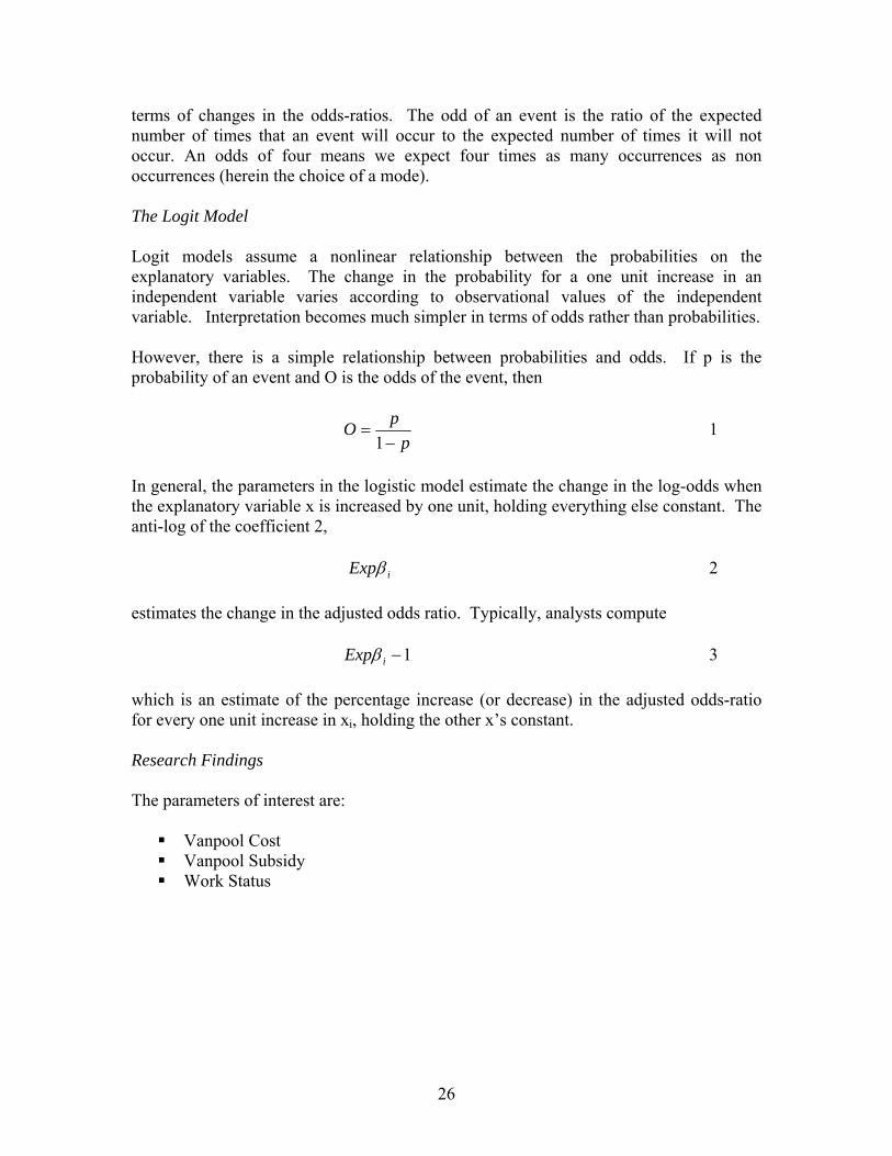
terms of changes in the odds-ratios. The odd of an event is the ratio of the expected number of times that an event will occur to the expected number of times it will not occur. An odds of four means we expect four times as many occurrences as non occurrences (herein the choice of a mode). The Logit Model Logit models assume a nonlinear relationship between the probabilities on the explanatory variables. The change in the probability for a one unit increase in an independent variable varies according to observational values of the independent variable. Interpretation becomes much simpler in terms of odds rather than probabilities. However, there is a simple relationship between probabilities and odds. If p is the probability of an event and O is the odds of the event, then

p

pO−

=1

1

In general, the parameters in the logistic model estimate the change in the log-odds when the explanatory variable x is increased by one unit, holding everything else constant. The anti-log of the coefficient 2,

iExpβ 2 estimates the change in the adjusted odds ratio. Typically, analysts compute

1−iExpβ 3 which is an estimate of the percentage increase (or decrease) in the adjusted odds-ratio for every one unit increase in xi, holding the other x’s constant. Research Findings The parameters of interest are:

Vanpool Cost Vanpool Subsidy Work Status

26

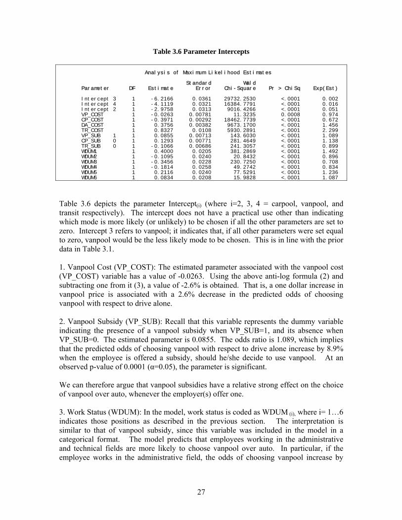
Table 3.6 Parameter Intercepts Analysis of Maximum Likelihood Estimates Standard Wald Parameter DF Estimate Error Chi-Square Pr > ChiSq Exp(Est) Intercept 3 1 -6.2166 0.0361 29732.2530 <.0001 0.002 Intercept 4 1 -4.1119 0.0321 16384.7791 <.0001 0.016 Intercept 2 1 -2.9758 0.0313 9016.4266 <.0001 0.051 VP_COST 1 -0.0263 0.00781 11.3235 0.0008 0.974 CP_COST 1 -0.3971 0.00292 18462.7739 <.0001 0.672 DA_COST 1 0.3756 0.00382 9673.1700 <.0001 1.456 TR_COST 1 0.8327 0.0108 5930.2891 <.0001 2.299 VP_SUB 1 1 0.0855 0.00713 143.6030 <.0001 1.089 CP_SUB 0 1 0.1293 0.00771 281.4649 <.0001 1.138 TR_SUB 0 1 -0.1066 0.00686 241.3057 <.0001 0.899 WDUM1 1 0.4000 0.0205 381.2869 <.0001 1.492 WDUM2 1 -0.1095 0.0240 20.8432 <.0001 0.896 WDUM3 1 -0.3456 0.0228 230.7250 <.0001 0.708 WDUM4 1 -0.1814 0.0258 49.2742 <.0001 0.834 WDUM5 1 0.2116 0.0240 77.5291 <.0001 1.236 WDUM6 1 0.0834 0.0208 15.9828 <.0001 1.087 Table 3.6 depicts the parameter Intercept(i) (where i=2, 3, 4 = carpool, vanpool, and transit respectively). The intercept does not have a practical use other than indicating which mode is more likely (or unlikely) to be chosen if all the other parameters are set to zero. Intercept 3 refers to vanpool; it indicates that, if all other parameters were set equal to zero, vanpool would be the less likely mode to be chosen. This is in line with the prior data in Table 3.1. 1. Vanpool Cost (VP_COST): The estimated parameter associated with the vanpool cost (VP_COST) variable has a value of -0.0263. Using the above anti-log formula (2) and subtracting one from it (3), a value of -2.6% is obtained. That is, a one dollar increase in vanpool price is associated with a 2.6% decrease in the predicted odds of choosing vanpool with respect to drive alone. 2. Vanpool Subsidy (VP_SUB): Recall that this variable represents the dummy variable indicating the presence of a vanpool subsidy when VP_SUB=1, and its absence when VP_SUB=0. The estimated parameter is 0.0855. The odds ratio is 1.089, which implies that the predicted odds of choosing vanpool with respect to drive alone increase by 8.9% when the employee is offered a subsidy, should he/she decide to use vanpool. At an observed p-value of 0.0001 (α=0.05), the parameter is significant. We can therefore argue that vanpool subsidies have a relative strong effect on the choice of vanpool over auto, whenever the employer(s) offer one. 3. Work Status (WDUM): In the model, work status is coded as WDUM (i), where i= 1…6 indicates those positions as described in the previous section. The interpretation is similar to that of vanpool subsidy, since this variable was included in the model in a categorical format. The model predicts that employees working in the administrative and technical fields are more likely to choose vanpool over auto. In particular, if the employee works in the administrative field, the odds of choosing vanpool increase by

27

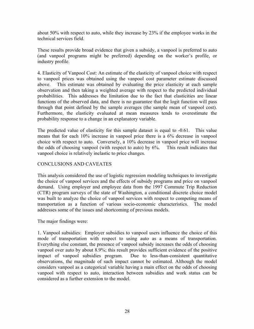
about 50% with respect to auto, while they increase by 23% if the employee works in the technical services field. These results provide broad evidence that given a subsidy, a vanpool is preferred to auto (and vanpool programs might be preferred) depending on the worker’s profile, or industry profile. 4. Elasticity of Vanpool Cost: An estimate of the elasticity of vanpool choice with respect to vanpool prices was obtained using the vanpool cost parameter estimate discussed above. This estimate was obtained by evaluating the price elasticity at each sample observation and then taking a weighted average with respect to the predicted individual probabilities. This addresses the limitation due to the fact that elasticities are linear functions of the observed data, and there is no guarantee that the logit function will pass through that point defined by the sample averages (the sample mean of vanpool cost). Furthermore, the elasticity evaluated at mean measures tends to overestimate the probability response to a change in an explanatory variable. The predicted value of elasticity for this sample dataset is equal to -0.61. This value means that for each 10% increase in vanpool price there is a 6% decrease in vanpool choice with respect to auto. Conversely, a 10% decrease in vanpool price will increase the odds of choosing vanpool (with respect to auto) by 6%. This result indicates that vanpool choice is relatively inelastic to price changes.

CONCLUSIONS AND CAVEATES This analysis considered the use of logistic regression modeling techniques to investigate the choice of vanpool services and the effects of subsidy programs and price on vanpool demand. Using employer and employee data from the 1997 Commute Trip Reduction (CTR) program surveys of the state of Washington, a conditional discrete choice model was built to analyze the choice of vanpool services with respect to competing means of transportation as a function of various socio-economic characteristics. The model addresses some of the issues and shortcoming of previous models. The major findings were: 1. Vanpool subsidies: Employer subsidies to vanpool users influence the choice of this mode of transportation with respect to using auto as a means of transportation. Everything else constant, the presence of vanpool subsidy increases the odds of choosing vanpool over auto by about 8.9%; this result provides sufficient evidence of the positive impact of vanpool subsidies program. Due to less-than-consistent quantitative observations, the magnitude of such impact cannot be estimated. Although the model considers vanpool as a categorical variable having a main effect on the odds of choosing vanpool with respect to auto, interaction between subsidies and work status can be considered as a further extension to the model.

28

2. Vanpool Price Elasticity: A weighted average vanpool price elasticity value was estimated. The calculated value is equal to -0.61. This value indicates that vanpool demand (with respect to auto) is relatively inelastic. These results have to be considered in the light of the dataset used to estimate the model. The model was constructed using the dataset as described in Section 1 of this study. Care should be exercised when considering the practical applicability of such results in a policy setting context. Data Analysis Using 1999 Data Set This section follows from the conclusions and caveats defined in the previous section. In this section, an additional dataset was taken into consideration and several modeling approaches were considered. Also, supplementary predictors were considered for potential inclusion in the model, as defined in the previous section. WHY CONSIDER ADDITIONAL PREDICTORS? An additional set of predictors was considered for inclusion in the model, specifically to test the use of:

Subsidy amounts instead of dummy variables Dummy variables indicating the industry sector of employment instead of a

dummy variable indicating the job position for the sample respondents The use of subsidies amount for carpool, vanpool, and transit was rejected due to the extremely low reported values in both the 1997 and 1999 sample. The dummy variables indicating the presence of a subsidy were instead retained. An analysis of the employer survey indicated that the respondents checked more than one answer when asked to which sector the surveyed firm belonged. Therefore, a set of dummies could not be created. The dummy variables indicating the job positions were instead retained in the model. These dummies were recoded due to a different set of questions of the 1999 survey with respect to the 1997. WHY USE THE 1999 DATASET? Researchers were interested in analyzing a more recent dataset to investigate the reliability of the model and congruency of parameter estimates. Therefore, a second dataset was built for the year 1999 using employer and employee data from the 1999 Commute Trip Reduction (CTR) program surveys of the state of Washington. The same approach used to build the 1997 dataset, as described in the previous section was used here as well.

29

DATA ANALYSIS Table 3.7 displays information on the mode choice frequencies of the employee survey. After resizing the dataset to account for auto, carpool, vanpool, and transit, and after eliminating reporting noise23, a total of 109,275 observations were retained. The employees were asked to report the mode choice of each day of the week they were surveyed. Since the modal split remained constant throughout the days of the week, only one day of the week was taken into consideration, specifically Tuesday (which tends to be a more typical commute week day). Table 3.7 shows that vanpool choice represents only 1.87% of the total number of respondents, compared to 1.98% in the 1997 dataset. That is, only 2,038 respondents used vanpool the week prior to the survey. Again, these percentages are constant throughout the days of the week.

Table 3.7 Mode Choice Frequencies – 1999 Dataset

Cumulative CumulativeMode Frequency Percent Frequency PercentAuto 75,098 68.72 75,098 68.72

Carpool 17,322 15.85 92,420 84.58Vanpool 2,038 1.87 94,458 86.44Transit 14,517 13.56 109,275 100.00

Table 3.8 displays some descriptive statistics for the sample and the Pearson correlation coefficients for the cost variables.

23 These include all sort of reporting errors as commonly encountered in survey instrument reporting.

30

Table 3.8 Pearson Correlations

Drive Alone Carpool Vanpool Transit Distance

Drive Alone 1.00 0.75 0.56 0.11 1.00

Carpool 0.75 1.00 0.42 0.09 0.75

Vanpool 0.56 0.42 1.00 0.08 0.56

Transit 0.11 0.09 0.08 1.00 0.11

Distance 1.00 0.75 0.56 0.11 1.00

Variable Mean Std Dev Minimum MaximumDrive Alone 4.74 2.31 1.75 14.12

Carpool 4.09 2.49 0.25 14.12

Vanpool 2.25 1.16 0.84 8.22

Transit 2.14 0.47 1.00 2.50

Pearson Correlation CoefficientsMode Costs

THE MODEL Multinomial Logit Model for 1999 dataset The next step was to run the multinomial logit on the 1999 dataset. The model assumption and characteristics are the same as those described in a previous section. Table 3.9 shows the result of the model.

31

Table 3.9 Model Results Model Fit Statistics Intercept Intercept and Criterion Only Covariates AIC 181366.73 78308.355 SC 181395.30 78708.369 -2 Log L 181360.73 78224.355 R-Square 0.6393 Max-rescaled R-Square 0.7670

Analysis of Maximum Likelihood Estimates Standard Wald Parameter MODE DF Estimate Error Chi-Square Pr > ChiSq Exp(Est) Intercept 3 1 -7.6668 0.2127 1299.6100 <.0001 0.000 VP_COST 3 1 -0.1603 0.0396 16.3925 <.0001 0.852 CP_COST 3 1 -0.6863 38.6182 0.0003 0.9858 0.503 DA_COST 3 1 1.0836 38.6182 0.0008 0.9776 2.955 TR_COST 3 1 0.9653 0.0846 130.1720 <.0001 2.626 VP_SUB 3 1 1.0270 0.0559 336.9553 <.0001 2.793 CP_SUB 3 1 -0.0342 0.0599 0.3257 0.5682 0.966 TR_SUB 3 1 -0.7892 0.0552 204.1220 <.0001 0.454 WDUM1 3 1 0.0511 0.1099 0.2157 0.6423 1.052 WDUM2 3 1 -0.5321 0.1249 18.1421 <.0001 0.587 WDUM3 3 1 -0.7043 0.1219 33.3639 <.0001 0.494 WDUM4 3 1 -0.6808 0.1578 18.6191 <.0001 0.506 WDUM5 3 1 -0.3750 0.1364 7.5559 0.0060 0.687 WDUM6 3 1 0.0115 0.1022 0.0128 0.9100 1.012

Parameter Inferences The model was estimated using drive alone as the base mode. That is, when interpreting the parameters, the comparison is between the effects of a given parameter on the choice of vanpool, carpool, and transit with respect to drive alone. Research Findings 1. Vanpool Cost (VP_COST): The estimated parameter associated with the vanpool cost (VP_COST) variable has a value of -0.1603. Using the anti-log formula (2):

iExpβ and subtracting one from it (3):

1−iExpβ a value of -14.8% is obtained. That is, ceteris paribus, a one dollar increase in vanpool price is associated with a 14.8% decrease in the predicted odds of choosing vanpool with respect to drive alone. This represents a significant departure from the 2.6% change estimated by the model using 1997 data.

32

2. Vanpool Subsidy (VP_SUB): This variable represents the dummy variable indicating the presence of a vanpool subsidy when VP_SUB=1, and its absence when VP_SUB=0. The estimated parameter is 1.02. The odds ratio is 2.79, which implies that the predicted odds of choosing vanpool with respect to drive alone increase by about 1.8 times when the employee is offered a subsidy, should he/she decide to use vanpool. At an observed p-value less 0.0001 (α=0.05), the parameter is significant. Vanpool subsidies have a relatively strong effect on the choice of vanpool over auto, whenever the employer(s) offers one. 3. Work Status (WDUM): In the model, work status is coded as WDUM (i), where i=1…6 indicates those positions as described in Table 3.10.

Table 3.10 Work Status Dummy Variables

Dummy Job Type

WDUM1 Administrative Support

WDUM2 Craft/Production/Labor

WDUM3 Management

WDUM4 Sales/Marketing

WDUM5 Customer Service

WDUM6 Other

The interpretation is similar to that of vanpool subsidy, since this variable was included in the model in a categorical format. The previous model predicted that employee working in the administrative and technical fields are more likely to choose vanpool over auto. The results using the 1999 dataset are not robust, since most of the estimated parameters associated with the dummies are not statistically significant. 4. Elasticity of Vanpool Cost : An estimate of the elasticity of vanpool choice with respect to vanpool prices was obtained using the vanpool cost parameter estimate discussed above. This estimate was obtained by evaluating the price elasticity at each sample observation and then taking a weighted average with respect to the predicted individual probabilities. This addresses the limitation due to the fact that elasticities are linear functions of the observed data, and there is no guarantee that the logit function will pass through that point defined by the sample averages (the sample mean of vanpool cost). Furthermore, the elasticities evaluated using means measures tends to overestimate the probability response to a change in an explanatory variable. The predicted value of elasticity for the 1999 sample dataset is equal to -1.34. This value means that for each 10% increase in vanpool price there is a 13.4% decrease in vanpool choice with respect to auto. Conversely, a 10% decrease in vanpool price will increase the odds of choosing vanpool (with respect to auto) by 13.4%.

33

MODEL IMPROVEMENT: THE NESTED LOGIT MODEL APPROACH One last approach that was tried in the analysis considers the application of a nested logit model. The nested logit model allows the user to consider the existence of different competitive relationships between groups of alternatives in a common nest. Such difference indicates that the effect of a change in an attribute of an alternative on the probability of that alternative depends on whether they are or are not in a common nest. This model represents a theoretical improvement upon the simple multinomial (conditional) logit model. The following nest was used to run the model:

Figure 3.11: Nested Logit Model Approach

Decision

Drive Alone Carpool Vanpool Bus/Transit

The assumption is that both drive alone and carpool are closed means of transportation, due to their mode specific characteristics. For example, the cost of auto differs from the cost of carpool only by the number of passengers sharing the ride while carpooling. Vanpool and transit represent “stand alone” modes. The results of the nested logit estimation are displayed in Table 3.11, the parameter estimated are displayed in Table 3.12. These results were obtained using the 1999 dataset.

34

Table 3.112 Nested Model Results The MDC Procedure Nested Logit Estimates Model Fit Summary Dependent Variable decision Number of Observations 101442 Number of Cases 405768 Log Likelihood -109138 Maximum Absolute Gradient 59.70997

The MDC Procedure

Nested Logit Estimates

Model Fit Summary Dependent Variable decision Number of Observations 101442 Number of Cases 405768 Log Likelihood -109138

The MDC Procedure

Nested Logit Estimates

Model Fit Summary

Maximum Absolute Gradient 59.70997 Number of Iterations 55 Optimization Method Newton-Raphson AIC 218291 Schwarz Criterion 218357

Discrete Response Profile Index mode Frequency Percent 0 1 69595 68.61 1 2 16154 15.92 2 3 1882 1.86 3 4 13811 13.61 Goodness-of-Fit Measures for Discrete Choice Models Measure Value Formula Likelihood Ratio (R) 344237 2 * (LogL - LogL0) Upper Bound of R (U) 562514 - 2 * LogL0 Aldrich-Nelson 0.7724 R / (R+N) Cragg-Uhler 1 0.9664 1 - exp(-R/N) Cragg-Uhler 2 0.9702 (1-exp(-R/N)) / (1-exp(-U/N)) Estrella 0.9947 1 - (1-R/U)^(U/N) Adjusted Estrella 0.9947 1 - ((LogL-K)/LogL0)^(-2/N*LogL0) McFadden's LRI 0.6120 R / U Veall-Zimmermann 0.9117 (R * (U+N)) / (U * (R+N)) N = # of observations, K = # of predictors

Table 3.13 Parameter Estimates

Parameter Estimates Standard Approx Parameter DF Estimate Error t Value Pr > |t| Gradient cost_L1 1 -0.0473 0.000701 -67.53 <.0001 -14.3618 CP_SUB_L1 1 -10.5522 3.0758 -3.43 0.0006 0.038535 VP_SUB_L1 1 -2.8251 1.5619 -1.81 0.0705 0.057639

35

The estimated cost parameter is statistically significant, with an observed p-value of less than 0.0001; the estimated parameter associated with vanpool subsidy is not statistically significant (α=0.05). Using the McFadden formula to derive an estimate of the direct elasticity for a mode outside the nest (such as vanpool):

(1-Pn)βXn 4 a weighted average of individual elasticities were computed across those individuals that chose vanpool in the sample data. This elasticity value is approximately -1.14. This value means that for each 10% increase in vanpool price there is an 11.4% decrease in vanpool choice across the group of individuals that chose vanpool. Conversely, a 10% decrease in vanpool price increases the group odds of choosing vanpool by 11.4%. This estimate of elasticity is much higher than that obtained with the simple multinomial logit model, indicating that vanpool is relatively elastic to price changes. Again, these results are dependent on the dataset used and the hypothesized nest. Other hypothetical nests could be conceived, each potentially leading to different elasticity estimates. Care should be exercised when considering the practical applicability of such results in a policy setting context. Conclusions This analysis considered the use of logistic regression modeling techniques to investigate the choice of vanpool services and the effects of subsidy programs and price on vanpool demand. Using employer and employee data from the 1999 Commute Trip Reduction (CTR) program surveys from the state of Washington, a conditional discrete choice model was built to analyze the choice of vanpool services with respect to competing means of transportation as a function of various socio-economic characteristics. The major findings from the 1999 data are: 1. Vanpool subsidies: Employer subsidies to vanpool users influence the choice of this mode of transportation with respect to using auto as a means of transportation. Everything else constant, the presence of vanpool subsidy increases the odds of choosing vanpool over the automobile by more than 1.8 times; this result provides sufficient evidence of the positive impact of vanpool subsidies program. Due to less-than-consistent quantitative observations, the magnitude of such impact cannot be estimated. Although the model considers vanpool as a categorical variable having a main effect on the odds of choosing vanpool with respect to auto, interaction between subsidies and work status can be considered as a further extension to the model. 2. Vanpool Price Elasticity: A weighted average vanpool price elasticity value was estimated. The calculated value is equal to -1.34. This value indicates that vanpool

36

demand is relatively elastic; when using a nested logit model, with car and carpool under as single nest, the estimated elasticity is approximately -1.14. These results have to be considered in the light of the dataset used to estimate the model. The model was constructed using the 1999 dataset. Care should be exercised when considering the practical applicability of such results in a policy setting context.

37

Chapter Four: Qualitative Analysis

As indicated before, once the ideal variables had been identified, a request for data was sent to rideshare organizations and vanpool agencies across the country through a listserv. Several responses were received but few followed up with data. Based on the project’s objectives, special effort was made to obtain more data from Florida organizations. The organizations were sent an electronic letter describing the scope of the study and a form that outlined the requested raw data for the elasticity model in detail. The organizations were further asked to note any changes in the cost to riders (increase in fare or change in subsidy where known). The agencies contacted were in particular asked to provide any additional comments that would lend insight into their respective operations and sites. However, because of the very low response from most rideshare organizations, only a qualitative analysis was possible for these sites. This ranged from a simple tabular representation of trends and correlations to a simple direct elasticity analysis. Simple Elasticity Analysis Case Studies A mid-point elasticity estimate was done for agencies that responded with a previous fare change in their data sent. These included VanGo from Colorado and VOTRAN and LYNX from Florida. The mid-point elasticites for these organizations were estimated by the following method: Vanpool Elasticity = ∆Ridership/∆Cost * Mean Cost/Mean Ridership Where: ∆Ridership = Change in ridership ∆Cost = Change in cost or fare Mean Cost = Average cost or fare Mean Ridership = Average ridership For example: First quarter simple direct elasticity for VanGo for 2001-2002 was:

(-5/(9.81)*(145.095/190.5)) = -0.38820262 This estimate measures the relative change (∆) in ridership given a change (∆) in the cost of vanpooling (the personal share of the van per month), thus measuring price sensitivity.

38

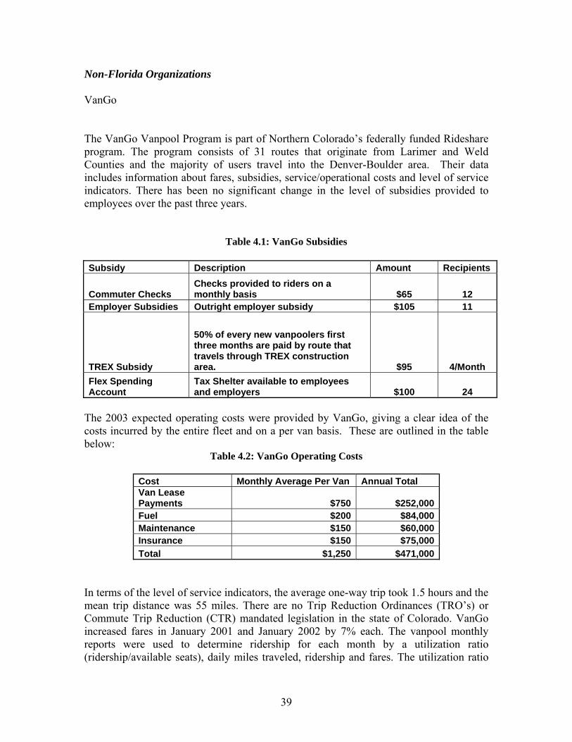
Non-Florida Organizations VanGo The VanGo Vanpool Program is part of Northern Colorado’s federally funded Rideshare program. The program consists of 31 routes that originate from Larimer and Weld Counties and the majority of users travel into the Denver-Boulder area. Their data includes information about fares, subsidies, service/operational costs and level of service indicators. There has been no significant change in the level of subsidies provided to employees over the past three years.

Table 4.1: VanGo Subsidies

Subsidy Description Amount Recipients

Commuter Checks Checks provided to riders on a monthly basis $65 12

Employer Subsidies Outright employer subsidy $105 11

TREX Subsidy

50% of every new vanpoolers first three months are paid by route that travels through TREX construction area. $95 4/Month

Flex Spending Account

Tax Shelter available to employees and employers $100 24

The 2003 expected operating costs were provided by VanGo, giving a clear idea of the costs incurred by the entire fleet and on a per van basis. These are outlined in the table below:

Table 4.2: VanGo Operating Costs

Cost Monthly Average Per Van Annual Total Van Lease Payments $750 $252,000 Fuel $200 $84,000 Maintenance $150 $60,000 Insurance $150 $75,000 Total $1,250 $471,000

In terms of the level of service indicators, the average one-way trip took 1.5 hours and the mean trip distance was 55 miles. There are no Trip Reduction Ordinances (TRO’s) or Commute Trip Reduction (CTR) mandated legislation in the state of Colorado. VanGo increased fares in January 2001 and January 2002 by 7% each. The vanpool monthly reports were used to determine ridership for each month by a utilization ratio (ridership/available seats), daily miles traveled, ridership and fares. The utilization ratio

39

was created from the availability of monthly ridership reports as a ratio of seats being used over the actual number of seats in each van. The average of this ratio for each respective quarter was made to correspond with the elasticity estimates. The adjusted elasticity estimates were calculated by multiplying the elasticity estimate by the average utilization ratio for each respective quarter. This gave an effective “elasticity” estimate based on the actual vanpool ridership. The following elasticity estimates were calculated as described above for the following time periods:

Table 4.3: VanGo Elasticities

Elasticity Estimates Utilization Ratio Adjusted Elasticity Measurement & Durations 2000/01 2001/02 2000/01 2001/02 2000/01 2001/02Short Term 1st Quarter

-1.279 -0.388 86.28% 82.73% -1.103 -0.321

Short Term 2nd Quarter

-1.939 -0.729 87.72% 79.88% -1.701 -0.583

Long Term -0.700 -0.678 88.19% 86.43% -0.633 -0.586 For example, the estimates drawn from ridership changes resulting from the first fare change in January 2001 were calculated by point elasticity and showed that for the short-term, elasticity value was less inelastic. The second change in January 2002 revealed the same pattern. However, long-term elasticity showed that ridership was fairly inelastic as riders were less sensitive to the price change. Thus, riders reacted minimally to the fare change in the long-run for FY 2001-2002. Similarly, in FY 2000-2001, the short-term estimates were more elastic than the long-term estimates, suggesting some underlying factors24 that may have increased ridership. To make adjustments in the estimates, a utilization ratio was created which is a capacity measure of average seats and average rides per month per van. The utilization ratios were then used to adjust the elasticity to give a more accurate measure of the effective price sensitivity of vanpool riders given the actual seats used in the van. Florida Agencies 1. VOTRAN: VOTRAN is a transit agency in Volusia County, Florida that also provides a vanpool service to its users. The agency provided data from FY 98-99 to FY 03-04 on passenger boardings, passenger seat miles, total vans, passenger miles driven and an estimate of commuter costs saved derived from a reduction in SOV trips.

24There are certain characteristics of vanpool operations besides fare changes which may affect the attraction of new riders, e.g., lay-offs, change in work hours and change in work location

40

Table 4.4: VOTRAN Operating Data

Category FY 98/99 FY 99/00 FY 00/01 FY 01/02 FY 02/03 FY 03/04

YTD Ridership 5652 10390 31019 30131 49752 13705 Passenger Seat Miles 411,675 631,741 1,961,405 1,659,640 1,847,434 622,586 Revenue Collected $8,327 $11,280 $51,030 $56,767 $61,979 $34,892 Total Miles Driven 51,552 59,172 263,591 211,248 212,176 140,152 Saved Commute Cost $119,385 $183,204 $568,807 $481,295 $535,755 $224,131 Total Vans in Service 3 3 11 14 14 19

During the data period, the fleet had an average growth rate of 73.5% and a fare change (from $28 to $30 of per person) in 2000. The fleet increased from three vans to eleven vans during that period. A simple elasticity estimate was done by isolating the effect of the fare change and looking at the change in ridership only from the three vans that were in operation before and after the change. The elasticity was estimated by using a direct number of users per van as reported in VOTRAN’s Vanpool and expense summary reports: Elasticity Estimate: = (-744/24)*(348/6372) = -1.69 The price elasticity of the vanpool service was -1.69 (fairly elastic) showing that riders responded to the fare change and a 10% increase in price would result in a 16.9% decline in vanpool ridership. In general, the other data attributes analyzed showed growth. Thus, total miles driven grew by 62.7%, passenger seat miles grew by 65%, and passenger boarding grew by 86.2%. Another proposed fare increase from $30 to $32 and an increase in the fleet with five new vans is scheduled to come online. 2. LYNX: LYNX is the public transit provider for the Orlando, Florida area. As part of its commuter assistance program, vanpool services are offered to large groups of commuters who arrive at work at the same time. The organization and implementation of service is monitored by LYNX. Data was provided on vanpool operations for FY 2001, FY 2002 and FY 2003 on ridership, passenger miles, commute distances and operating expenses. The table below shows the breakdown of operating expenses incurred for FY 2002:

Table 4.5: LYNX Operating Data

Operating Expense $729,418 Operating Expense Per Capita $0.51 Operating Expense Per Peak Vehicle $13,763 Operating Expense Per Passenger Trip $3.32 Operating Expense Per Passenger Mile $0.09 Operating Expense Per Revenue Miles $0.55 Operating Expense Per Revenue Hour $26.51

41

A fare change was made on January 1st, 2002 where the cost increased from $460 to $490. A short-term elasticity comparing ridership in December 2001 to April 2002 was done. The estimates were as follows:

Table 4.6: LYNX Elasticities Duration Calculation Elasticity Short-Term Elasticity (Quarter 1) (16/0.73)*(43.55/204) 4.6792 Long-Term Elasticity (2001/2002) (15/8.84)*(522.54/928.5) 0.95494 Long-Term Elasticity (2002/2003) (-51/8.84)*(522.54/1507.5) -1.9997 The estimates shown are based on the same vans in December 2001 compared with those in April 2002. Holding the number of vans constant, the positive elasticity for both the short-term and the long-term shows that there are other factors, possibly job growth, seasonality or some other variable that led to this change. For example, according to LYNX feedback, NAVAIR (a defense company) was brought on board at a time when rate changes were made in its contract with VPSI (a vanpool service provider). NAVAIR completely subsidized vanpool expenses for their federal employees which may have caused an increase in ridership observed during that short-term period. When elasticity is estimated for the calendar year of 2002 in comparison with 2003 (using the lagged effect of the initial fare change in January 2002), a fairly elastic estimate is observed. When the $30 cost increase is shared by van users, it averages $0.73 per rider per month. It appears that since the mean vanpool cost per rider per month was $47.11, a $0.73 cost increase may not have a strong impact. In terms of subsidy levels, it was reported that one vanpool group was totally subsidized by their employer (18 passengers), and the Navy subsidized three vanpools for their employees 23 passengers, with subsidies ranging from $61.25- $70.00. One other agency provided a partial subsidy of $32.66 (Days Suites Hotel). Tabular Analysis Case Studies For some of the agencies that submitted data without any evidence of recent fare or subsidy changes, a tabular analysis was used to simply provide a sense of trends and correlation among variables. However, no elasticity analysis was possible since there was not enough information, i.e., no change in the fare or subsidy. These included C-Tran in Vancouver Washington and Spokane transit in Spokane Washington. Florida participating organizations included Manatee County Government, VPSI Melbourne, Commuter Services of North Florida (CSNF), South Florida Commuter Services (SFCS) and Bay Area Commuter Services (BACS). Non-Florida Organizations 1. C-Tran: C-Tran, a transit agency in Vancouver, Washington indicated that there had been no change in their leasing rates for vanpools and therefore no elasticity estimate was possible. However, a tabular analysis was done. They provided three years of operational data (1999-2001) including revenue miles, number of vans in operation and cost/benefit (revenue/expenses) of the operation. The table below summarizes the

42

operational costs and mileage during the three years discussed above. However, C-Tran noted that ridership was higher on subsidized vans relative to the rest of the fleet.

Table 4.7: C-Tran Operating Data

Year Average Vans Miles Revenue Expenses

Net Revenue

1999 17 286,482 $128,730 $304,496 ($175,766) 2000 15 249,255 $113,119 $250,245 ($137,126) 2001 11 157,981 $84,825 $183,426 ($98,601)

2. Spokane Transit: Spokane Transit in Spokane, Washington provided van specific data for their fleet from January 2003 to December 2003 on ridership, revenue miles and hours and miles per hour. Similarly, since the fare for vanpoolers had not changed, elasticity estimates could not be done. The table below shows the variance in ridership, vans in operation and other variables for service in 2003.

Table 4.8: Spokane Operating Data

Month Mean Riders Per Van

Revenue Miles

Revenue Hours Ridership Vans

Mean Round Trip (miles)

January 10.8 28132 858 8419 31 50February 10.8 28588 816 8281 32 50March 10.8 30167 869 9002 32 47April 11 30908 902 8884 32 47May 10.8 29339 890 8449 32 46June 10.9 29272 829 8441 33 44July 11 29528 876 8384 33 43August 10.4 28173 830 7977 33 41September 10.8 30442 888 8700 33 44October 10.8 31822 930 9357 32 45November 11.5 26463 749 8097 31 47December 11.7 30227 897 8435 32 46

The variance in ridership, vans in operation and other variables arose from differences in routes for each van and ridership demand. There were thirty –two vans in operation. The cost was $0.24 per mile (including tires, fuel, maintenance, parts and insurance). The mean roundtrip trip distance was forty-seven miles and it took an hour on average. Monthly subsidies provided to riders ranged from $25-$35 on fares that range from $30-$62 per rider. Florida Organizations 1. Manatee County Government: Manatee County Government operated two vanpools that operate between Manatee and Sarasota Counties; one van runs between Brandon and

43

Bradenton and currently has four commuters (service began in September 1998). The other van runs between Sarasota and Bradenton and has five commuters (service began in July 1999). A fee of $2 per day ($1 per trip) is charged to its users. The Brandon vanpool saw an increase of 3% between FY 00-01 and FY 01-02 in its average ridership per day. The table below (1.1) shows the average daily ridership and its growth during the years in operation.

Table 4.9 Brandon Vanpool

Month FY00-01 FY01-02 FY02-03 October 4.13 4.6 4.6 November 4.1 4.72 4.15 December 3.16 4 4.56 January 5.85 3.9 4.66 February 4.21 4.42 3.31 March 3.59 4.9 3.69 April 4.57 3.7 3.69 May 3.61 4.2 3.64 June 3.5 3.95 3.52 July 4.05 4.6 2.07 August 4.65 3.89 3.1 September 4.7 5 3 Mean 4.176667 4.323333 3.665833 Growth Rate 0.035116 -0.15208 -0.05848

However, between FY 01-02 and FY 02-03 there was a decline in average daily ridership in the van by 15%. The range of ridership indicates that the slight variance in ridership during that period from 4.32 to 3.66 may just have been due to one rider leaving the van for a host of other reasons. There was also a subsequent decline in total round trips and the total number of days the van was in operation between FY 00-01 and FY 01-02 and the FY 01-02 and FY 02-03. The Sarasota vanpool showed a decrease in average ridership per day between FY 00-01 and FY 01-02 by 11.59% with the month of March 2002 having 2.65 commuters per day (the mean was 4.02). The next fiscal year between 01-02 and 02-03 there was also a decline but it was 1.3%. The table below shows the average daily ridership and its growth during the years in operation. Similar to the Brandon vanpool, there was on average a decline between the fiscal years of data provided.

44

Table 4.10 Sarasota Vanpool

Month FY00-01 FY01-02 FY02-03 October 3.77 4.9 4.3 November 4.15 4.89 4.17 December 3.87 3.5 4.05 January 5.6 4.38 4.42 February 4.78 3.7 3.68 March 4.77 2.65 4.05 April 3.75 4 4.59 May 5 3.6 4.28 June 5.38 4.05 3.67 July 4.52 4.36 3.86 August 4.52 4.05 3.48 September 4.5 4.2 3.09 Mean 4.550833 4.023333 3.97 Growth Rate -0.11591 -0.01326

2. VPSI-Melbourne: VPSI is a one of the oldest and largest vanpool operators in the United States. The Brevard Vanpool Program is an important part of Space Coast Area Transit’s (SCAT) commuter choice program (a public/private partnership between VPSI and SCAT). Vans are purchased by the County Commission with Federal capital grants and are provided by VPSI. Users pay for all operating costs. The current cost of a van is $440 per month, including full maintenance and insurance (gas excluded). Brevard vanpools are currently operating 175,000 miles per month, making 8000 trips and carrying approximately 30,000 passengers. There are also commuter vans and demand responsive vans within the fleet. Data was provided for FY 2001, FY 2002 and FY 2003, including revenue miles, passengers, trips and the number of vans. The table provides a summary of the monthly averages for each fiscal year for the variables provided.

Table 4.11: VPSI-Melbourne Operating Data Variable FY 2001 FY 2002 FY 2003 Miles 80814.91 75277 78387.42Trips 765.92 1345.83 1376.83Passengers 5758.41 5249 5208.42Passenger Miles 600346.17 549309.58 546269.33Vans 34.33 32.42 32.5Passenger Per Mile 14.09 14.35 15.11Passengers Per Van 167.62 162.09 160.19Miles Per Trip 106.19 55.98 57.32Miles Per Van 2354.16 2325.90 2411.69Passengers Per Van/Day 7.62 7.37 7.28Cost Per Rider (Monthly) $ 58.24 $ 59.72 $ 60.73 Cost Per Rider (Daily) $ 2.65 $ 2.73 $ 2.76

45

3. South Florida Commuter Services: South Florida Commuter Services is a regionally funded commuter assistance program that operates in the Miami-Dade Area in South Florida. The vanpool program includes development of new vanpools and technical assistance. The program offers a complete vanpool package that includes vehicle insurance, comprehensive maintenance and an Emergency Ride Home (ERH) program. The Miami-Dade MPO is one of the major partners in the provision of the South Florida Vanpool Program (SFVP) that has been in operation since 1998. The partnership includes the Florida Department of Transportation (funding), the Miami-Dade MPO (contract management), VPSI, Inc. (operations, vehicles, maintenance and insurance) and SFLCS (outreach/marketing). Data was provided both on an annual basis (mined by monthly totals) and in a summary format over the six year life of the vanpool service. The data includes annual reports on the number of vanpool programs in the area, passenger trips saved (by group and by month), passenger miles saved (by group and by month) and aggregated emissions reductions for the year, vehicle miles traveled and detailed data on fuel usage. The annual numbers give an indication of seasonality that may arise in service and in operations. However, in reviewing the annual numbers from year to year, the variance in these numbers is simply a function of the number of passengers in a given group. The summary of all five years shown below, show an average growth rate of the groups being 80% per year, over the five years with sharp peaks between 1999-2000 (183%) and 2000-2001 (129.4%), when the largest growth in vanpool groups occurred.

Table 4.12: SFCS Operating Data

Year Active Groups

Pass Trips Saved Pass. Miles Saved

Avg. Parking Spaces Saved

1998 5 14420 462438 291999 6 21746 627429 422000 17 45820 1324974 892001 39 145432 5236671 2822002 53 172575 5511351 3092003 69 210358 6530042 385

South Florida Commuter Services marketing efforts focused on matching programs involving the targeting of employers to form work groups as opposed to direct contact with individuals. There was a increase in the subsidy provided by the MPO to SFLCS from $300 to $400 though the other factors mentioned above were the key contributing factors to vanpool service expansion. Vanpool groups with one participant commuting in or out of Miami-Dade County receive a monthly subsidy of $400.00 from the Miami-Dade MPO. The van fares are based on mileage and on the size of the group. Their reported average roundtrip commute distance is sixty miles per day, an average of eight riders per van and a total of seventy-two vans in the fleet. SFCS also has a list of companies that offer incentives to induce commuters to consider mode shifting towards more “environmentally friendly” modes of transportation. These include:

46

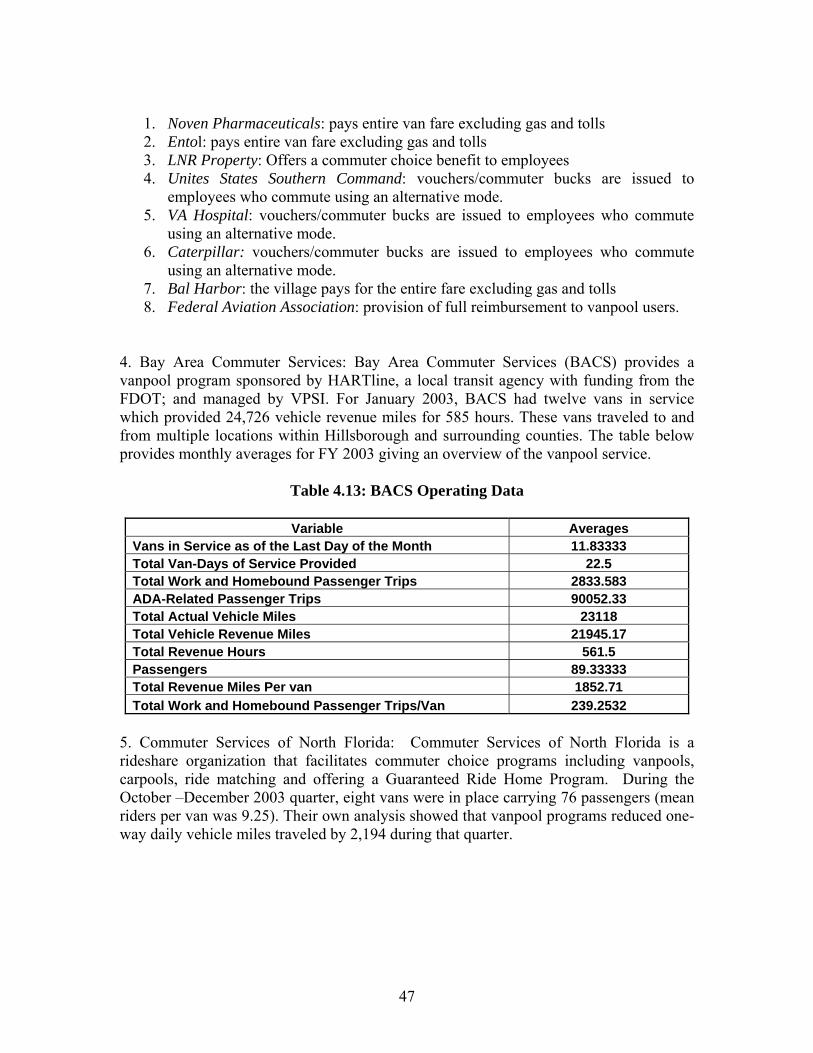
1. Noven Pharmaceuticals: pays entire van fare excluding gas and tolls 2. Entol: pays entire van fare excluding gas and tolls 3. LNR Property: Offers a commuter choice benefit to employees 4. Unites States Southern Command: vouchers/commuter bucks are issued to

employees who commute using an alternative mode. 5. VA Hospital: vouchers/commuter bucks are issued to employees who commute

using an alternative mode. 6. Caterpillar: vouchers/commuter bucks are issued to employees who commute

using an alternative mode. 7. Bal Harbor: the village pays for the entire fare excluding gas and tolls 8. Federal Aviation Association: provision of full reimbursement to vanpool users.

4. Bay Area Commuter Services: Bay Area Commuter Services (BACS) provides a vanpool program sponsored by HARTline, a local transit agency with funding from the FDOT; and managed by VPSI. For January 2003, BACS had twelve vans in service which provided 24,726 vehicle revenue miles for 585 hours. These vans traveled to and from multiple locations within Hillsborough and surrounding counties. The table below provides monthly averages for FY 2003 giving an overview of the vanpool service.

Table 4.13: BACS Operating Data

Variable Averages Vans in Service as of the Last Day of the Month 11.83333 Total Van-Days of Service Provided 22.5 Total Work and Homebound Passenger Trips 2833.583 ADA-Related Passenger Trips 90052.33 Total Actual Vehicle Miles 23118 Total Vehicle Revenue Miles 21945.17 Total Revenue Hours 561.5 Passengers 89.33333 Total Revenue Miles Per van 1852.71 Total Work and Homebound Passenger Trips/Van 239.2532

5. Commuter Services of North Florida: Commuter Services of North Florida is a rideshare organization that facilitates commuter choice programs including vanpools, carpools, ride matching and offering a Guaranteed Ride Home Program. During the October –December 2003 quarter, eight vans were in place carrying 76 passengers (mean riders per van was 9.25). Their own analysis showed that vanpool programs reduced one-way daily vehicle miles traveled by 2,194 during that quarter.

47

Chapter Five: Concluding Observations and Recommendations Unlike the transit industry whose sensitivity to price changes tends to be limited, the vanpool industry tends to face volatile conditions and is therefore more likely to be very elastic. First, increases in transit fares tend to be very small, often creeping at a gingerly rate ranging from $0.05 to $0.25. Because of the minor nature of such increases, the reactions tend to be minimal. Secondly, transit riders for most urban areas tend to be captive riders who may not easily change modes due to changes in fares (their elasticity is possibly influenced more by changes in income rather than fares). Similarly, for transit choice riders (who are typically influenced by the level of service than cost), because of the insignificance of the amount of fare changes, they may not be influenced to switch modes. However, one of the challenges facing the vanpool users is the “tipping point” problem where the cost for one or more of the pool members may be at the break even point. Since vanpool users tend to cover all or a large portion of their direct cost (capital and operating), their fares tend to be large. Consequently, since they absorb a large share of the cost, their fare changes tend to be fairly large. There is also potential for a “double dip effect” where the user may not only be affected by the fare increase but also, should one or more of the users drop out, their cost has to be shared with the remaining members whose burden is now larger than the original fare increase. Naturally, this fare increase along with the potential loss of a member may prompt each of the remaining members to consciously or unconsciously explore other alternative modes. The more the members explore other alternatives, the higher the probability of losing more members and the higher the possibly of dissolving the pool. Because of this interdependence among pool members, the reactions to fare changes are likely to be volatile, i.e., dropout of one member may mean dropout of all other members.

Evidence of Growth Trends In general, the data so far collected appear to indicate a growing trend in the vanpool program in two ways. First, the existing programs have continued to grow in size. Secondly, the industry as a whole, continue to grow with new starts. The former is supported by secondary data from the National Transit Database25 which shows vanpool vehicle growth of almost 9 times over a period of 18 years from 447 vehicles in 1984 to 3932 vehicles in 2001 as shown in the table below.

25 National Transit Database data on the Florida Transit Information System Version 2003 CD-ROM produced by Florida International University for Florida DOT.

48

Table 5.1: Growth Trends

Year Total Year Total 1984 447 1993 1227 1985 488 1994 1503 1986 524 1995 1533 1987 581 1996 1919 1988 661 1997 2545 1989 486 1998 3329 1990 612 1999 3580 1991 930 2000 3692 1992 1045 2001 3932

Similarly, as shown in the trends below, several new starts are evident especially in the periods of 1987-1991 and 1998-1999. These growth trends not only complicates the measurement of elasticity, i.e., the influence of fares/subsidy on ridership variability, but also creates volatile elasticity results that are difficult to generalize with a rule of thumb.

Figure 5.2 National Trends

1

10

100

1000

1984 1985 1986 1987 1988 1989 1990 1991 1992 1993 1994 1995 1996 1997 1998 1999 2000 2001

AnchorageArlington HeightsAustinBirminghamBostonBradentonBremertonCharlotteCOCOACorpus ChristiDes MoinesDouglasvilleFort MyersFort WorthGarden GroveGrand PrairieGrand RiverGranite CityGreenvilleHamptonHonoluluHoustonHuntsvilleKansas CityLakelandLorainLynnwoodMariettaMelbourne

Sum of Vehicles Operated in Maximum Service

Year

Location

49

Potential Opportunities

These and other related factors may help explain why vanpool users appear to exhibit higher elasticities. Therefore, one way for mitigating volatility among pool members is for the provision of a safety net to sustain existing members while they search for a new member. It is also important when evaluating the success of vanpool programs, especially with respect to transit, to note that due to public subsidy for transit operating costs, the average recovery ratio for transit is typically a little over 20% and may be even lower for express bus service (which is comparable to a vanpool type of service). From a policy perspective therefore, because vanpool users pay most of their operating costs, public policy measures for sustaining declining membership groups need to be given serious consideration.

Analytical Findings

This analysis considered the use of logistic regression modeling techniques to investigate the choice of vanpool services and the effects of fare changes and subsidy programs on vanpool demand. Using employer and employee data from the 1997 and 1999 Commute Trip Reduction (CTR) program surveys from the state of Washington, a conditional discrete choice model was built to analyze the choice of vanpool services with respect to competing means of transportation as a function of various socio-economic characteristics. The major findings were: 1. Vanpool subsidies: Employer subsidies to vanpool users influence the choice of this mode of transportation with respect to using auto as a means of transportation. Therefore, holding everything else constant, the presence of vanpool subsidy increases the odds of choosing the vanpool over the automobile. This result provides sufficient evidence of the positive impact of vanpool subsidies program. 2. Vanpool Price Elasticity: A weighted average vanpool price elasticity value was estimated. The calculated values indicated that vanpool demand is relatively elastic; especially when using a nested logit model, with car and carpool under a single nest.

Model Specific Limitations

Results from the logit model have to be considered in the light of the dataset used to estimate the model. The model was constructed using only data from the Puget Sound and therefore care should be exercised when considering the practical applicability of such results in a policy setting context. Similarly, results from the nested logit model are dependent on the dataset used and the hypothesized nest. Other hypothetical nests could be conceived, each potentially leading to different elasticity estimates. Care should therefore be exercised when considering the practical applicability of such results in a policy setting context.

50

General Limitations of the Study

Because of the limited scope of data (from a regional perspective) and a short history of the study of elasticity in the vanpool industry, this study does not provide a silver bullet with which one can make conclusive explanations. Unlike the transit industry which for a while could count on the Simpson-Curtin rule of thumb, the limited scope of data makes it difficult to provide a more generalized application of findings. However, the study provides a framework from which subsequent studies can employ diverse research and refine the methodologies towards more reliable results. These would include a wide representation of participating regions, a rich longitudinal collection of data, and a significant amount of large and small fare changes to provide an adequate data base for analysis.

51

References _______________ Heteroscedasticity and Binary Dependent Variable Models- http://www.emory.edu/POLS/zorn/Classes/POLS585AU02/notes4-1.pdf _______________ Discrete Dependent Variable Model- http://gulliver.trb.org/publications/nchrp/cd-22/v2chapter5.html _______________ http://www.indiana.edu/~statmath/stat/all/cat/2c1.html _______________ http://www.gseis.ucla.edu/courses/ed231c/notes3/mlogit1.html _______________ http://www.albany.edu/csda/nomreg.pdf American Public Transit Association. 1995. 1994-95 Transit Fact Book. Washington, DC. American Public Transit Association. 1991. Fare Elasticity and Its Application to Forecasting Transit Demand. Washington, DC. Andrle, S. “Coordinated Intermodal Transportation Pricing and Funding Strategies”. Research Results Digest. Number 14- October 1997 Apogee Research, Inc. 1994. The Costs of Transportation: Final Report. Prepared for the Conservation Law Foundation. Beshers, Eric. 1994. External Costs of Automobile Travel and Appropriate Policy Responses. Highway Users Federation, Washington, DC. Bhatt, Kiran U. 1994. Potential of Congestion Pricing in the Metropolitan Washington Region. In Transportation Research Board Special Report 242. Volume 2. TRB, National Research Council, Washington, DC, pp. 62-88. Cameron, Michael. 1991. Transportation Efficiency: Tackling Southern California's Air Pollution and Congestion. Environmental Defense Fund, Regional Institute of Southern California. Center for Urban Transportation Research. 1993. Parking and Transit Policy Study. Prepared for the Florida Department of Transportation, May 1993. Center for Urban Transportation Research. 1994. Southeast Florida Regional Transit Fare Coordination Study. Prepared for Palm Beach County Transportation Authority/Broward County Transit/Metro-Dade Transit Agency/Tri-County Commuter Rail.

52

Charles River Associates, Inc. 1995. Strategies for Influence Choice of Urban Travel Mode. Phase I Interim Report. TCRP Project H-4A. Dargay, J and Hanly, M. “Report To The Department of the Environment; Transport and the Regions- Bus Fare Elasticities”. www.ucl.ac.uk/~ucetmah/exec.htm Deakin, Elizabeth. 1994. Urban Transportation Congestion Pricing: Effects on Urban Form. In Transportation Research Board Special Report 242. Volume 2. TRB, National Research Council, Washington, DC, pp. 334-355. DeCorla-Souza, Patrick, and J.D. Gupta. 1989. Evaluation of Demand- Management Strategies for Toledo's Year 2010 Transportation Plan. In Transportation Research Record 1209. National Research Council, Washington, DC, pp. 1-15. Domencich, Thomas and Gerald Kraft. 1970. Free Transit. D.C. Heath, Lexington, Massachusetts. Ecosometrics, Inc. 1980. Patronage Impacts of Changes in Transit Fares and Services. Fabricatore, D. York, B., Prowda, B. Winters, P. and Cleland, F. “Puget Sound Region Vanpool Market Assessment, Final Report”. Presented To Washington State DOT. February 25th, 1999 Federal Railroad Administration. 1993. Environmental Externalities and Social Costs of Transportation Systems- Measurement, Mitigation and Costing: An Annotate Bibliography. Office of Policy, Washington, DC. Gillen, David. 1994. Peak Pricing Strategies in Transportation, Utilities, and Telecommunications: Lessons for Road Pricing. In Transportation Research Board Special Report 242. Volume 2. TRB, National Research Council, Washington, DC, pp. 115-151. Glaister, Stephen and David Lewis. 1978. An Integrated Fares Policy for Transport in London. Journal of Public Economics, vol. 9, pp. 341-355. Goodwin, P.B. 1992. A Review of New Demand Elasticities with Special Reference to Short and Long Run Effects of Price Changes. Journal of Transport Economics and Policy, vol. 26, no. 2, pp. 155-163. Harris, A, Thomas, R and Boyle, D. “Metropolitan Atlanta Rapid Transit Authority Fare Elasticity Model”- Journal of the Transportation Research Board- No. 1669. September 1999

53

Harvey, Greig. 1979. STEP--Short- Range Transportation Evaluation Program: Description and User's Guide. Metropolitan Transportation Commission, Oakland, California. Hensher, D. “Establishing A Fare Elasticity Regime For Urban Passenger Transport”. Journal of Transport Economics and Policy. Volume 32, Part 2. August 1997 Hensher, D and Raimond, T. “Estimation of Public Transportation Fare Elasticities in the Sydney Region”. Pricing and Regulation Tribunal of New South Wales. October 1996 Kain, John. 1994. Impacts of Congestion Pricing on Transit and Carpool Demand and Supply. In Transportation Research Board Special Report 242. Volume 2. TRB, National Research Council, Washington, DC, pp. 502-553. Kemp, M. “ Building Transit Ridership- An Exploration of Transit’s Market Share and The Public Policies That Influence It”. TCRP Report 27-Chpt 4 pp.34-38. September 1997 Kulash, Damian. 1973. Parking Taxes for Congestion Relief: A Survey of the San Francisco Experience. Report 1212-91. The Urban Institute, Washington, DC. Lago, Armando M., Patrick Mayworm, and Jonathan McEnroe. 1992. Transit Ridership Responsiveness to Fare Changes. Traffic Quarterly, vol. 35, no. 1 (January). Lee, Douglass B. 1992. A Market- Oriented Transportation and Land-Use System: How Different Would It Be? Conference on Privatization and Deregulation in Passenger Transport. Tampere, Finland (June 1991). Linsalata, J and Pham, L. “Fare Elasticity and Its Application to Forecasting Transit Demand”. American Public Transit Association. August 1991 Litman, Todd. 1995. Transportation Cost Analysis: Techniques, Estimates and Implications. Victoria Transport Policy Institute, Victoria, B.C. MacKenzie, James J., Roger C. Dower, and Donald D.C. Chen. 1992. The Going Rate: What It Really Costs to Drive. World Resources Institute, Washington, DC. Massachusetts Bay Transportation Authority. 1992. Draft Environmental Impact Report on the 1991 Fare Increase. Boston, Massachusetts. Mayworm, Lago and McEnroe. “Patronage Impacts of Changes in Transit Fares and Services”. UMTA-DOT 1980

54

Metropolitan Planning Council. 1994. Mobility for Metropolitan Chicago: An Expanded Role for Public Transit. Final Report of the Regional Public Transportation Task Force. Chicago, Illinois. Multisystems, Inc., et al. 1995. TCRP Report 10: Fare Policies, Structures, and Technologies TRB, National Research Council, Washington, DC. 1996. Nelson, Dick and Don Shakow. 1995. Least Cost Planning: A Tool for Metropolitan Transportation Decision Making. Prepared for Transportation Research Board, 74th Annual Meeting January 22-28), Washington, DC. Olson, David J. 1994. Pricing Urban Roadways: Administrative and Institutional Issues. In Transportation Research Board Special Report 242. Volume 2. TRB, National Research Council, Washington, DC, pp. 216-249. Oum, T, Waters, W. and Yong, J. “A Survey of Recent Estimates of Price Elasticities of Demand For Transport”- Policy, Planning and Research Working Papers- Transportation. WPS 359-January 1990 Pickrell, Don. 1991. The Role of Parking Charges in Highway Congestion Pricing. Testimony presented to the U.S. Senate Subcommittee on Water Resources, Transportation, and Infrastructure. Portland State University. 1994. Policy Options to Attract Auto Users to Public Transportation. TCRP Project H-3 Interim Report (unpublished). Pucher, John. 1995. Budget Cutters Looking at Wrong Subsidies. Passenger Transport (March 13), p. 3. Rom, Mark. 1994. The Politics of Congestion Pricing. In Transportation Research Board Special Report 242. Volume 2. TRB, National Research Council, Washington, DC, pp. 280-299. Shoup, Donald C. 1994. Cashing Out Employer-Paid Parking: A Precedent for Congestion Pricing? In Transportation Research Board Special Report 242. Volume 2. TRB, National Research Council, Washington, DC, pp. 152-199. Shoup, Donald C. and Richard W. Willson. 1992. Employer-Paid Parking: The Problem and Proposed Solutions. Transportation Quarterly vol. 46, no. 2, pp. 169-192. Steiner, R.L. 1992. Lessons for Transportation Demand Management from Utility Industry Demand-Side Management (Abridgment). In Transportation Research Record 1346, TRB, National Research Council, Washington, DC, pp. 14-17.

55

TCRP Web Document 12 (Project B-12). “Traveler Response to Transportation System Changes”. Contractor’s Interim Handbook. March 2000 U.S. General Accounting Office. 1992. Mass Transit: Effects of Tax Changes on Commuter Behavior. GAO/RCED- 92243. Washington, DC. Voith, R. “The Long-Run Elasticity of Demand for Commuter Rail Transportation”- Journal of Urban Economics. Vol.30 (1991), pp.360-372 (www.urbanfutures.org/abstract.cfm) Willson, R. and D. Shoup. 1990. The Effect of Employer-Paid Parking in Downtown Los Angeles: A Study of Office Workers and Their Employers, Southern California Association of Governments, Los Angeles, California. Willson, R. and D. Shoup. 1990. Parking Subsidies and Travel Choices: Assessing the Evidence, Transportation, Volume 17, pp. 141-157. Willson, R. 1992. Estimating the Travel and Parking Demand Effects of Employer Paid Parking, Regional Science and Urban Economics, Volume 22, pp. 133-145. Winters, P. and Cleland, F. “Vanpool Pricing and Financing Guide”. Center For Urban Transportation Research. Wuestefeld, Norman and Edward Regan, III. 1981. Impact of Rate Increases on Toll Facilities. Traffic Quarterly (October).

56

APPENDIX: Data Fields Based on Elements of Survey Questions

Field Name Data

type Description

1 RecNum Number Scanned record number 2 Ncsserial Text serial number for scanning batch 3 Ncsbatch Text batch number 4 Ncsdate Text scanner date 5 Nreligemp Text number of eligible employees 6 Hdnumsurs Text number of surveys scanned 7 Hdcounty Text county code 8 County Number county ID 9 Hdcity Text City code

10 CTRID Text worksite CTR ID 11 survey type Text type of survey 12 Affecode Text Affected employee? A=affected, N=non-affected 13 Quesresp Text raw scan file data

14 ITEM1 Number Do you usually work 35 or more hours per week for this employer in a

position intended to last 12 months or more? 1= yes, 2=no

15 Item2 Number Are you scheduled to arrive, or do you usually arrive, at your work

location between 6 and 9 a.m.? 1=yes, 2=no

16 Item3_mon Number Last week did you arrive at work on Monday between 6 and 9 a.m.?

1=yes, 2=no.

17 Item3_tues Number Last week did you arrive at work on Tuesday between 6 and 9 a.m.?

1=yes, 2=no.

18 Item3_weds Number Last week did you arrive at work on Wednesday between 6 and 9 a.m.?

1=yes, 2=no.

19 Item3_thur Number Last week did you arrive at work on Thursday between 6 and 9 a.m.?

1=yes, 2=no.

20 Item3_fri Number Last week did you arrive at work on Friday between 6 and 9 a.m.?

1=yes, 2=no.

21 Item3_none Number Last week did you arrive at work no days between 6 and 9 am.? 1=yes,

2=no.

22

Item4a_mon Number Last Monday, what type of transportation did you use to commute to your usual work location? 1= drive alone, 2=carpool, 3=vanpool, 4=motorcycle, 5=bus/transit, 6=bicycle, 7=walked, 8=telecommuted, 9=other, 10=DNW.

23

Item4a_tues Number Last Tuesday, what type of transportation did you use to commute to your usual work location? 1= drive alone, 2=carpool, 3=vanpool, 4=motorcycle, 5=bus/transit, 6=bicycle, 7=walked, 8=telecommuted, 9=other, 10=DNW.

24

Item4a_weds Number Last Wednesday, what type of transportation did you use to commute to your usual work location? 1= drive alone, 2=carpool, 3=vanpool, 4=motorcycle, 5=bus/transit, 6=bicycle, 7=walked, 8=telecommuted, 9=other, 10=DNW.

25

Item4a_thur Number Last Thursday, what type of transportation did you use to commute to your usual work location? 1= drive alone, 2=carpool, 3=vanpool, 4=motorcycle, 5=bus/transit, 6=bicycle, 7=walked, 8=telecommuted, 9=other, 10=DNW.

26 Item4a_fri Number Last Friday, what type of transportation did you use to commute to

57

your usual work location? 1= drive alone, 2=carpool, 3=vanpool, 4=motorcycle, 5=bus/transit, 6=bicycle, 7=walked, 8=telecommuted, 9=other, 10=DNW.

27 Item4b Number If you are in a carpool or vanpool, how many people (age 16 or older)

are usually in the vehicle, including yourself? 28 Item4c Number Was last week a typical week for commuting?

29

Item5 Number Do you work five days a week, or do you have an alternative schedule? 1=5 days a week, 2=3 days a week, 3=4 days a week, 4=7 days in 2 weeks, 5=9 days in 2 weeks, 6=other.

30 Item6a Number Do you work at home for this employer and eliminate a commute trip?

(telecommuting) 1=yes, 2=no. 31 Item6b Number On how many days did you telecommute in the last two weeks?

32 Item6c Number Where do you telecommute? 1=home, 2= satellite or telework center,

3=other

33 Item7a_100 Number How many miles do you commute one-way from home to your usual

work location? 1=over 100 miles.

34 Item7a_99 Number How many miles do you commute one-way from home to your usual

work location?

35 Item7b Number What is this distance based on? 1= a measurement, 2=a sure estimate,

3= unsure estimate

36

Item8 Number What type of job do you do for this employer? 1=admin support, 2=craft/production, 3=farming, 4=labor, 5=management, 6=sales/marketing, 7=information/counter, 8=personal services. 9=social/public services 10=technical, 11=other

37 Item9 Number What is your home zip code 38 q10_a Number 0 - not marked, 1- employer car 39 q10_b Number 0 - not marked, 1 - lunch errands 40 q10_c Number 0 - not marked, 1 - ride home 41 q10_d Number 0 - not marked, 1 - meet mode change 42 q10_e Number 0 - not marked, 1 - financial incentive 43 q10_f Number 0 - not marked, 1 - parking cashout 44 q10_g Number 0 - not marked, 1 - special pool parking 45 q10_h Number 0 - not marked, 1 - help forming pool 46 q10_I Number 0 - not marked, 1 - special bicycle parking 47 q10_j Number 0 - not marked, 1 - showers/lockers 48 q10_k Number 0 - not marked, 1 - child care/banking/dry cleaning 49 q10_l Number 0 - not marked, 1 - on site food/kitchen 50 q10_m Number 0 - not marked, 1 - help reading bus schedule 51 q10_n Number 0 - not marked, 1 - more frequent bus service at worksite 52 q10_o Number 0 - not marked, 1 - more commute info 53 q10_p Number 0 - not marked, 1 - other

54 q11_car Number 0 - not marked, 1 - do now, 2 - likely, 3 - not likely, 4 - not an option, 5

- invalid

55 q11_van Number 0 - not marked, 1 - do now, 2 - likely, 3 - not likely, 4 - not an option, 5

- invalid

56 q11_tran Number 0 - not marked, 1 - do now, 2 - likely, 3 - not likely, 4 - not an option, 5

- invalid

57 q11_bicy Number 0 - not marked, 1 - do now, 2 - likely, 3 - not likely, 4 - not an option, 5

- invalid

58 q11_walk Number 0 - not marked, 1 - do now, 2 - likely, 3 - not likely, 4 - not an option, 5

- invalid

59 q11_tele Number 0 - not marked, 1 - do now, 2 - likely, 3 - not likely, 4 - not an option, 5

- invalid 60 q11_cww Number 0 - not marked, 1 - do now, 2 - likely, 3 - not likely, 4 - not an option, 5

58

- invalid 61 q12a1 Number 0 - not marked or 0, 1 - 1-99 trips taken 62 q12a2 Number 0 - not marked or 0, 1 - 1-99 trips taken 63 q12a3 Number 0 - not marked or 0, 1 - 1-99 trips taken 64 q12a4 Number 0 - not marked or 0, 1 - 1-99 trips taken 65 q12b1 Number 0 - not marked or 0, 1 - 1-99 trips taken 66 q12b2 Number 0 - not marked or 0, 1 - 1-99 trips taken 67 q12b3 Number 0 - not marked or 0, 1 - 1-99 trips taken 68 q12b4 Number 0 - not marked or 0, 1 - 1-99 trips taken

59