public investment strategies for regional development: an analysis based on optimization and...

IEEE TRANSACTIONS ON SYSTEMS, MAN, AND CYBERNETICS, VOL. SMC-6, NO. 3, MARCH 1976 165

Public Investment Strategies for RegionalDevelopment: An Analysis Based onOptimization and Sensitivity ResultsDONALD A. HANSON, MEMBER, IEEE, WILLIAM R. PERKINS, FELLOW, IEEE, AND

JOSE B. CRUZ, JR., FELLOW, IEEE

Abstract-Two strategies for regional development are analyzed: one than demand factors [13], [31], [41]. Supply factors typi-with an emphasis on public investment in the region's infrastructure and cally include public and private capital facilities and servicesthe other with an emphasis on public investment in education and training, and labor force size and quality. Supply factors are im-A growth model is presented which includes the effects of these public antbecause the d the capply fathe regioninvestment policy variables on productivity, private investment, and portant because they determine the capacity of the regionmigration. Alternative public investment strategies are evaluated using for production; they also play an important role in thea social welfare function. Optimization results indicate that a heavy region's adapting to changing demand patterns and inemphasis on education and training is a better strategy, at least for the attracting new private investment [39].specific problem considered. The sensitivity of the policy variables isinvestigated with respect to model parameter values, the region's initial Sme t ical devel deat with varou com-state, the tradeoff weights in the social welfare function, and the assump- ponents of the regional development problem [12], [34],tion that key model parameters are nonrandom. Assuming that a para- [38]. However, in this paper several components of thismeter is random implies the result that public investment in infrastructure problem are integrated into a large model, which must beshould be slightly increased from a low nominal level. solved numerically.

I. INTRODUCTION The model is intended to represent a region characterizedby the following conditions.

flEGIONAL development strategies have received con- 1) Socially and politically it is prepared to accept in-tur siderable attention inte o i l ing st creased industrialization and development. It is assumedture [8], [16], [18], [33]. A popular strategy is to invest that entrepreneurs will emerge if economic opportunitiesheavily in public overhead capital to generate investment exit.eTisesrteefrs aitl phase of opment[2]opportunities in the region for private investment [8], [18]. 2) The region has an acute shortage of private capitalPublic overhead capital is defined as that portion of the so ane relative oe supl oftabor present inds

publcly wnedcapial sock hichcontibuts tothestock and a relative over supply of labor. Its present indus-

publicly owned capital stock which contributes to the try is ofthe labor intensive, low-wage type.economic productivity of the region. Examples of overhead 3) There is a lack of adequate investment in both humancapital are transportation facilities, public utilities, and resources and public overhead capital compared withpublic oflice buildings. advanced regions.An alternative strategy for regional development is to 4) The underdeveloped region is economically linked to

emphasize investment in human resources through educa- an advanced region, which determines the wage rate differ-tion and training programs [18], [29]. In the long run, one ential and the interest rate and provides a source of moreexpects increases in labor productivity and the attraction advanced technology available to the underdevelopedof higher wage, more capital intensive activities. However, region. Historically, the Southeast region in the Unitedthis strategy is attendant with medium-run increases in out- States has possessed these characteristics [18], t29], [36].migration, a situation which frequently worries regional The model is calibrated for the Southeast region over thepolicy makers [17], [18]. Of course, as Hirschman points period 1940-1970.'out, investment in human resources and overhead capital In this paper, public investment in human resources andare both important for the development of a lagging region overhead capital are the control variables. The case is notThe problem is to sequence these investments in some considered in which public investment is allowed in directlyoptimal manner, perhaps emphasizing one type of public productive activities [25]. Regional development strategies

Amdlsdteautpb*investment i are evaluated using a social welfare function which dependsA model used to evaluate public investment strategies on per capita consumption [23], direct consumer benefitsmust represent the long-run development process of the of public overhead capital [32], and other benefits ofregion. Generally such models are based on supply rather education and training [40]. The results indicate that

emphasizing education and training initially is the betterManuscript received January 1, 1975, revised October 2, 1975.D. A. Hanson is with the Department of City and Regional Planning

and the Department of Electrical Engineering, Ohio State University, ' The 12-state Southeast region was defined for statistical purposesColumbus, Ohio 43210. by the U.S. Department of Commerce, Office of Business Economics,W. R. Perkins and J. B. Cruz, Jr. are with the Department of as Alabama, Arkansas, Florida, Georgia, Kentucky, Louisiana,

Electrical Engineering and the Coordinated Science Laboratory, Mississippi, North Carolina, South Carolina, Tennessee, Virginia,University of Illinois, Urbana, Ill. 61801. and West Virginia.

166 IEEE TRANSACTIONS ON SYSTEMS, MAN, AND CYBERNETICS, MARCH 1976

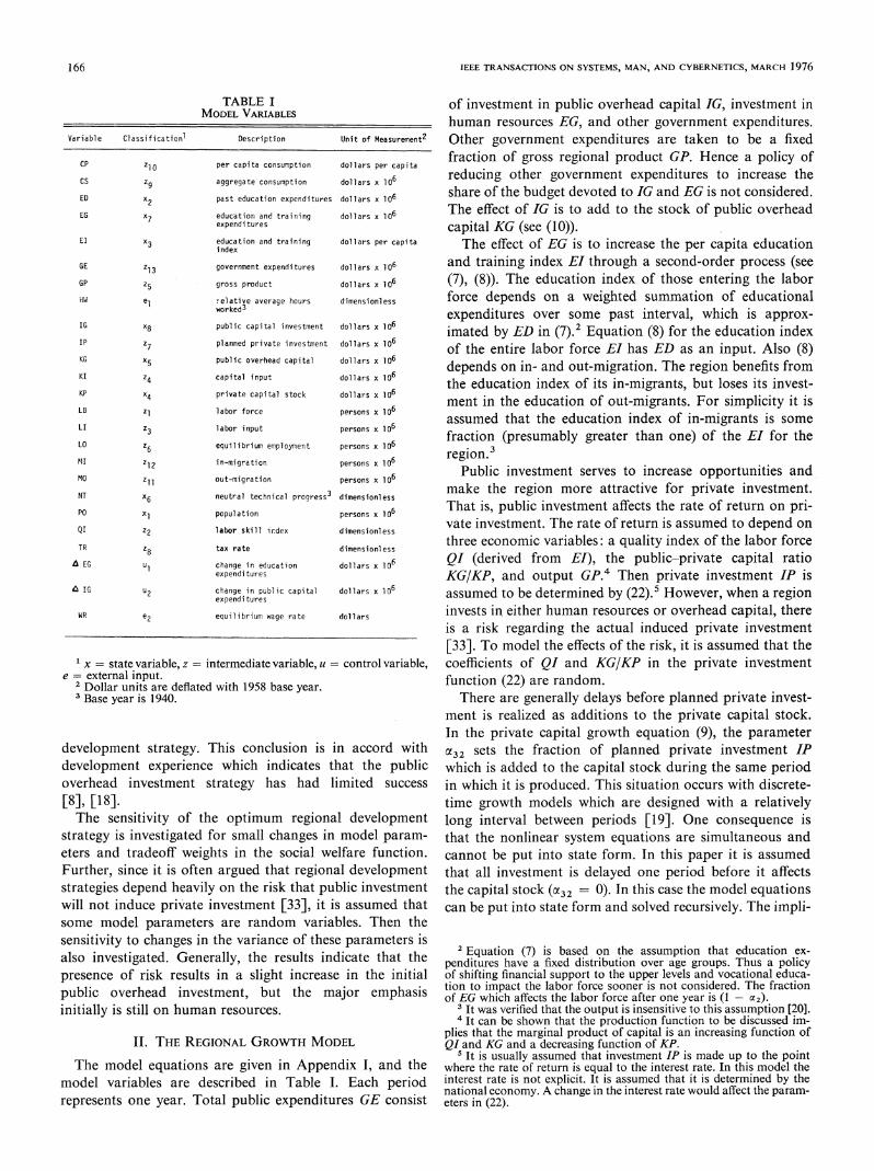
TABLE I of investment in public overhead capital IG, investment inMODEL VARIABLEShuman resources EG, and other government expenditures.

Variable Classification1 Description Unit of Measurement2 Other government expenditures are taken to be a fixed

CP Zio per capita consumption dollars per capitafraction of gross regional product GP. Hence a policy of

psagrercapita consumption dollars pr ca6 reducing other government expenditures to increase theCS zgaggregate consumption dollars x 106bdeto"an EGintcnser.

E9 ~ pat eucaionexpeditresdolarsx 16 share of the budget devoted to IG and EG is not considered.EG 2pasteducationandxtraindin dollars x 106 The effect of IG is to add to the stock of public overheadEG X7 education and training dollars x 106

expenditures capital KG (see (10)).

El x3 education and train-ing dollars per capita The effect of EG is to increase the per capita educationindex

GE z13 government expenditures dollars x 106 and training index EI through a second-order process (seeGP z5 gross product dollars x 106 (7), (8)). The education index of those entering the laborHW el relative average hours dimensionless force depends on a weighted summation of educational

worked3 expenditures over some past interval, which is approx-IG ug public capital investment dollars x 106 imated by ED in (7).2 Equation (8) for the education indexIP z7 planned private investment dollars x 1067P planned private innestoent dollars x 106 of the entire labor force EI has ED as an input. Also (8)KG X5 public overhead capital dollars x 106 depends on in- and out-migration. The region benefits fromKI z4 capital input dollars x 106KIZ4 capital input dollars x 106

the education index of its in-migrants, but loses its invest-KP x4 private capitalatockodolarslxlars. . .0.LB

4 paboriv forcapi stock pdollarso x 106 ment in the education of out-migrants. For simplicity it isLI z labor force persons x 106 assumed that the education index of in-migrants is some

LI l31abor i nput persons x 10 (peualohn6fteE h3~~~~~~~~~~~fraction (presumably greater than one) of the EI for theLO z6 equilibrium employment persons x 106 f 3

MI z12 in-migration persons x 106 region.

MO Zii out-migration persons x 106 Public investment serves to increase opportunities andNT x6 neutral technical progress3 dimensionless make the region more attractive for private investment.PO0 Xi population persons x 106 That is, public investment affects the rate of return on pri-QI Z2 labor skill irdex dimensionless vate investment. The rate of return is assumed to depend on

TR z tax rate dimensionless three economic variables: a quality index of the labor forceEG u1 change in education dollars 610 QI (derived from El), the public-private capital ratioA EG U chanexpnendicatron andas 1

expenditures KG/KP, and output GP.4 Then private investment IP is4 IG u2 change in public capital dollars x 106 assumed to be determined by (22).5 However, when a region

expenditCures

WR e2 equilibrium wiage rate dollars invests in either human resources or overhead capital, thereis a risk regarding the actual induced private investment[33]. To model the effects of the risk, it is assumed that the

x = state variable, z = intermediate variable, u = control variable, coefficients of QI and KG/KP in the private investmente = external input.

2 Dollar units are deflated with 1958 base year. function (22) are random.3 Base year is 1940. There are generally delays before planned private invest-

ment is realized as additions to the private capital stock.In the private capital growth equation (9), the parameter

development strategy. This conclusion is in accord with a32 sets the fraction of planned private investment IPdevelopment experience which indicates that the public which is added to the capital stock during the same periodoverhead investment strategy has had limited success in which it is produced. This situation occurs with discrete-[8], [18]. time growth models which are designed with a relativelyThe sensitivity of the optimum regional development long interval between periods [19]. One consequence is

strategy is investigated for small changes in model param- that the nonlinear system equations are simultaneous andeters and tradeoff weights in the social welfare function. cannot be put into state form. In this paper it is assumedFurther, since it is often argued that regional development that all investment is delayed one period before it affectsstrategies depend heavily on the risk that public investment the capital stock (a32 = 0). In this case the model equationswill not induce private investment [33], it is assumed that can be put into state form and solved recursively. The impli-some model parameters are random variables. Then thesensitivity to changes in the variance of these parameters isalso investigated. Generally, the results indicate that the penditures have a fixed distribution over age groups. Thus a policypresence of risk results in a slight increase in the initial of shifting financial support to the upper levels and vocational educa-pulcoverhead investment, but the major emphasis tion to imipaCfctthe labocrforcesoner is not considered. The fraction

initially is still on human resources. 3It was verified that the output is insensitive to this assumption [20].4 It can be shown that the production function to be discussed im-

plies that the marginal product of capital is an increasing function ofII. THE REGIONAL GROWTH MODEL QI and KG and a decreasing function of KP.

5It is usually assumed that investment IP is made up to the pointThe model equations are given in Appendix I, and the where the rate of return is equal to the interest rate. In this model the

model variables are described in Table I. Each period interest rate is not explicit. It is assumed that it is determined by thenational economy. A change in the interest rate would affect the param-represents one year. Total public expenditures GE consist eters in (22).

HANSON et al.: PUBLIC INVESTMENT STRATEGIES 167

cations Of %32 > 0 for public investment and regional 8000 _ -mgrowth rate are discussed elsewhere [19]. J

Aggregate consumption CS is determined from the-Education and T-rai'ning/identity x 6000 |- Expernd jtLires (rEG )Ing /d

GP Public Capital /GP = CS + IP + GE.

_ Expenditures (IG)0 5000_ _

To focus on supply factors, it is assumed that private invest- Xment is financed from sources in the region and that net c4000 - I

exports are zero. 30,Also it is assumed that the region is producing at capacity, -,

an assumption frequently made to study economic growth 2000[13]. The maximum output of the region GP is given by a Lconstant elasticity of substitution production function 1000

(CES) in (20) [4], [37]. The factors of production are labor 0_._/ _l _l _linput LI and capital input KI. Unemployment is assumed to 0 5 10 15 20 25 30be zero. However, if there is an "oversupply" of labor in Time (years)the region, then the marginal productivity of labor will be Fig. 1. Public investment series used to calibrate the model.low. This situation might be interpreted as one of under-employment [29]. The CES production function is chosento represent the possibility of substitution between capital for a developing region which can draw upon the experienceand labor. Numerically, the elasticity of substitution is and technology ofmore advanced regions [25, pp. 33-35].assumed to be 0.4. Economic and population growth are closely relatedThe capital input to production KI is a function of public through migration. Economic theory suggests and the

and private capital stocks (see (19)). In a developing region migration literature confirms that a critical variable inthe marginal product of capital input KI may be high, but determining migration flows is the expected economicdue to a severe shortage of public overhead capital KG, the return from the relocation [6], [35]. The expected economicmarginal product of private capital KP may be low. That is, return is usually measured in terms of wage rate differentialsthe absence of KG limits private investment opportunities assuming full employment or a combination of wage rate[33]. In general, public capital increases the efficiency of and unemployment differentials [28]. The model presentedprivate capital through the provision of transportation here assumes unemployment is zero. However, the regions'systems and other public services [25]. It might also be wage rate can be imputed assuming an ideal labor market.claimed that agglomeration economies can be obtained Suppose labor is hired up to the point where its marginalonly with sufficient infrastructure for metropolitan develop- value (derived from the production function) is equal to thement [39]. Whereas this assumption is realistic, it is not wage rate [23]. The wage rate is determined to yield fullformally included in the model since the CES production employment. Let WR(k) be the equilibrium wage rate atfunction has constant returns to scale. which net migration is approximately zero. It need not beThe labor input to production LI is the labor force LB the wage rate of the other regions if there are amenities in

adjusted for average hours worked HWand for labor quality the developing region. Let LO be the equilibrium labor(or skill level) QI (see (18)). The labor force LB is taken to force which would be fully employed if wages were WR. Itbe a fixed fraction of the regional population. The average is assumed that both in- and out-migration depend on thenumber of effective hours worked per person is assumed to difference (LO - LB). In-migration is assumed to be lineardecline at a fixed rate according to (14) [11, pp. 35-41]. The in this term, but empirical studies indicate that out-quality index QI is a function of the education and training migration is not linear. That is, for small or positive valuesindex El. It is assumed that QI increases monotonically of (LO - LB), relocation may not depend heavily on thiswith EI, but QI approaches an asymptote for large values term [28]. However, for a large relative oversupply of labor,of EI (see (17)) [11]. empirical evidence indicates that out-migration increases

For given capital and labor inputs, the gross regional rapidly as (LO - LB) decreases [17]. The migration func-product GP may increase over time due to technical prog- tions selected are (26) and (27). Out-migration is alsoress. In the production function (20) it is assumed that the assumed to increase with education and training [17].technical progress NT is neutral [37]. Technical progress Education and training may be related to the availabilitycan be due to efficiency gains such as improved administra- of information about opportunities elsewhere, the profici-tion or organization of production. It can also be due to the ency in job skills needed to take advantage of the oppor-introduction of new technology which generally requires tunities, and the costs of adjustment [35].new private investment. Hence the rate of neutral technical The parameters in the model were estimated from timeprogress is assumed to depend on the portion of new private series data between 1940 and 1970 constructed for the U.S.investment compared with the capital stock (see (11)). This Southeast region. The actual policies used during this periodformulation assumes that improved technology is available are shown in Fig. 1. Expenditures on education and trainingif investment occurs. This assumption is probably realistic EG are defined as total public and private expenditures on


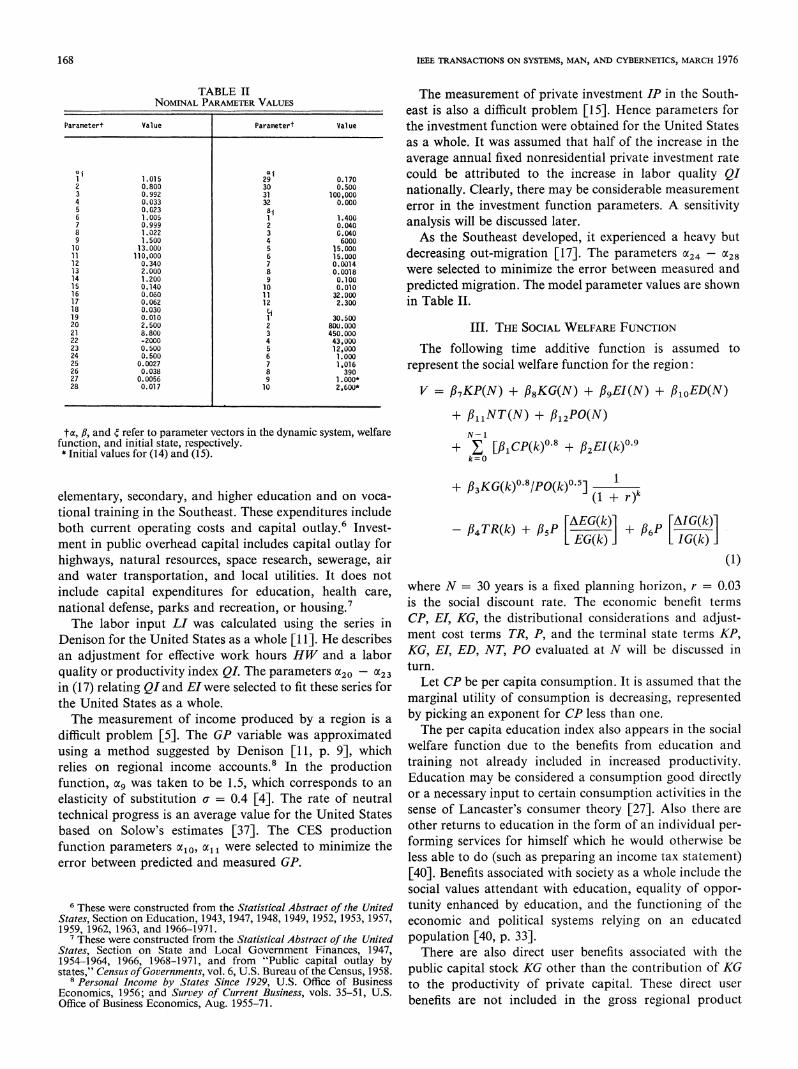
TABLE II The measurement of private investment IP in the South-NOMINAL PARAMETER VALUESNom__NAL_PARAMETER_VA_u___s east is also a difficult problem [15]. Hence parameters for

Parametert Value Parametert Value the investment function were obtained for the United States

as a whole. It was assumed that half of the increase in theaverage annual fixed nonresidential private investment rate

ci 1.015 0.170 could be attributed to the increase in labor quality QI2 0.800 30 0.500 nationally. Clearly, there may be considerable measurement3 0.992 31 100,0004 0.033 32 0.000 error in the investment function parameters. A sensitivity6 1.009 1.400 analysis will be discussed later.8 1.022 3 0.0409 1.500 4 6000 As the Southeast developed, it experienced a heavy but

11 110°00 15.000 decreasing out-migration [17]. The parameters a24 - 02812 0.340 7 0.001413 2.000 .8 0.0018 were selected to minimize the error between measured and14 1.200 9 0.10015 0.140 10 0.010 predicted migration. The model parameter values are shown16 0.060 11 32.00017 0.062 12 2.300 in Table II.18 0.03019 0.010 1 30.500

21 82800 3 450.000 III. THE SOCIAL WELFARE FUNCTION22 -2000 4 43,00023 0.500 5 12,000 The following time additive function is assumed to24 0.500 6 1.00025 0.0027 7 1,016 represent the social welfare function for the region:26 0.038 8 39027 0.0056 9 1.000*28 0.017 10 2,600* V = f37KP(N) + JJ8KG(N) + fB9EI(N) + 310ED(N)

+ 311NT(N) + /312PO(N)ta, Al, and f refer to parameter vectors in the dynamic system, welfare N- 1

function, and initial state, respectively. + E [#/CP(k)08 + EIl(k)09*Initial values for (14) and (15). k=2\

+ f33KG(k)08/1P0(k)0-:] 1elementary, secondary, and higher education and on voca- ( + r)ktional training in the Southeast. These expenditures includeboth current operating costs and capital outlay.6 Invest- - 4TR(k) + 5P 'AEG(k) + j6p A G(k)]ment in public overhead capital includes capital outlay for EG(k) IG(k)highways, natural resources, space research, sewerage, air (1)and water transportation, and local utilities. It does notinclude capital expenditures for education, health care, where N = 30 years is a fixed planning horizon, r = 0.03national defense, parks and recreation, or housing.7 is the social discount rate. The economic benefit termsThe labor input LI was calculated using the series in CP, EI, KG, the distributional considerations and adjust-

Denison for the United States as a whole [11]. He describes ment cost terms TR, P, and the terminal state terms KP,an adjustment for effective work hours HW and a labor KG, EI, ED, NT, PO evaluated at N will be discussed inquality or productivity index QI. The parameters 20- 023 turn.in (17) relating QI and EI were selected to fit these series for Let CP be per capita consumption. It is assumed that thethe United States as a whole. marginal utility of consumption is decreasing, representedThe measurement of income produced by a region is a by picking an exponent for CP less than one.

difficult problem [5]. The GP variable was approximated The per capita education index also appears in the socialusing a method suggested by Denison [11, p. 9], which welfare function due to the benefits from education and

relies on regional income accounts.8 In the production training not already included in increased productivity.function, oca was taken to be 1.5, which corresponds to an Education may be considered a consumption good directlyelasticity of substitution af = 0.4 [4]. The rate of neutral or a necessary input to certain consumption activities in thetechnical progress is an average value for the United States sense of Lancaster's consumer theory [27]. Also there arebased on Solow's estimates [37]. The CES production other returns to education in the form of an individual per-function parameters xlo, xll were selected to minimize the forming services for himself which he would otherwise beerror between predicted and measured GP. less able to do (such as preparing an income tax statement)

[40]. Benefits associated with society as a whole include thesocial values attendant with education, equality of oppor-

6 These were constructed from the Statistical Abstract of the United tunity enhanced by education, and the functioning of theStates, Section on Education, 1943, 1947, 1948, 1949, 1952, 1953, 1957, economic and political systems relying on an educated1959, 1962, 1963, and 1966-1971.

7 These were constructed from the Statistical Abstract of the United population [40, p. 33].States, Section on State and Local Government Finances, 1947, There are also direct user benefits associated with the1954-1964, 1966, 1968-1971, and from ";Public capital outlay bystates," Census ofGovernments, vol. 6, U.S. Bureau of the Census, 1958. public capital stock KG other than the contribution of KG

8 Personal Income by States Since 1929, U.S. Office of Business to the productivity of private capital. These direct userEconomics, 1956; and Survey of Culrrent Business, vols. 35-51, U.S.befisaentncudinhegosrinlpoutOffice of Business Economics, Aug. 1955-71.beeisaentncud hegosrgnlpout


oos policies can be evaluated. The terminal state components in

2:1

the social welfare index are the capital stocks KP and KG,the education index states EI and ED, neutral technicalprogress NT and population PO. The terminal population

0 o /is given a positive weight although, alternatively, a regionmight choose to seek a population target based on a prior

_ optimization or an ad hoc goal./0.05 The tradeoff weights in the social welfare function

-005 f-1-f12 are based on the authors' subjective judgment0LO / about tradeoffs which the U.S. Southeast region might find

acceptable. The weights f2 and f3 on the per capita educa-/6 6 l |tion index and public overhead capital were chosen to give-0.10

-n6-3 p 3 6 equal weight to their respective terms normalized by his-Chonge in Expenditures (Nrcent) torical values of these terms.

Fig. 2. Decreasing expenditures cost function (smooth curve) andits asymptotes. IV. OPTIMAL CONTROL PROBLEM AND RESULTS

The social welfare function (1) is implicitly in the formaccounts, and therefore these services should be includedin the social welfare function [3]. It is assumed that the flow V = S(x(N)) + E Lk(x(k),u(k),)(2)of direct services from KG is proportional to the stock k=Odivided by population to some power less than one. That is, where x is a state vector with components specified in Tablethere is congestion or lack of perfect access associated with I, u is the control vector representing changes in policythe stock KG. It is assumed that the marginal social welfare.. ~expenditures, and ,B iS a parameter vector. Equations (14)-associated with these services is decreasing and this is repre- (27) are used to eliminate intermediate and external vari-sented by an exponent on KG less than one. ables denoted by z and e, respectively, in Table 1.10Note that out-migration should not be included in the The discrete-time, dynamic, nonlinear system equations

social welfare function (1). That is, all groups (nonmi-The dicee-ie dyamc nlierstmeqaos

social wlaefnin()Th isaldescribing the growth of the region are implicitly in thegrants and migrants) receive greater economic benefits formfrom policies which maximize (1), not depending on out-migration. x(k + 1) =fk(x(k),u(k),L) (3)The social welfare function also depends on distributional for the case in which the investment lag parameter232 = 0.

considerations and adjustment costs [22]. It has beenarguedthatthsconsiderationsad djsmncosts [22. it d been Again (14)-(27) are used to eliminate intermediate variables.argued that these considerations should be Included early The system (3) is eighth order. The initial state x(0) = 4 isin the planning process [24], [30]. The intertemporal assumed to be a known vector of regional stock variablesincome distribution considerations are implemented by (see Table II).penalizing high tax rates in the social welfare function. AAdmissible control sequences are defined to be those forThis approach works since the problem with income dis- w

tribution ocur intal.hnotma aig ae nwhich expenditures EG and IG are nonnegative. The prob-tribution occurs initially when optimal savings rates and lem is to find an admissible control sequence which max-

hence tax rates are high. imizes (2) subject to (3) [7].The adjustment costs are associated with decreasing Optimalexpenditurepolicies are shown in Fig. 3 for two

public expenditures in either the education or public facili- the ex with nolcoss associatediwithgdecreasingcases: the case with no costs associated with decreasingties sectors, such as the cost of retraining labor which

switches between sectors. The cost function P (see Fig. 2) costs are imposed (f5 = f6 = 15). The case with theseis assumed to be a hyperbolic function which has little effect adjustment costs will be used as a reference and referred toon increases in expenditures but penalizes the percentage as the "nominal optimal solution" or simply as the "nom-decrease in expenditures: inal solution" (see the curves in Fig. 3 which are approx-

P(v) = -(v - 1v2 + 2 x 10-4). imately piecewise constant).Relative to the nominal solution the case without adjust-

In economic planning problems there is generally no ment costs has these properties: for three periods totalnatural terminal time N [9]. If a finite terminal time is expenditures are increased slightly and for seven periodschosen, the value of the terminal state must then be assessed. total expenditures are decreased slightly. Total output avail-This value is derived from the fact that society's welfare able for consumption over the ten-year period is increasedfollowing the planning horizon will be based upon the slightly. Initially, education and training expenditures areassets which it inherits. The terminal time N should besufficiently long so that the long run effects of the initial

10 To solve the optimization problem in this section and the sensitivityproblem in the following section does not require that the intermediatevariables be explicitly eliminated through substitution. All derivatives

9 The penalty function approach was selected to simplify the sen- required for solving necessary conditions can be calculated using thesitivity algorithm used in this research (see [19]). chain rule.


10,000 225,000

--- Capital Input (KI)9,000 __ 200,000 -Private Capital Stock (KP) /

.00 0_ -*-Public Capital Stock (KG) /175,000 -/

0~~~~~~~~~~~~~~~~~~~~~~~~~~~~~~~~~~~~~°7,000n,, 150,000 X

o \ ~~~~~~~~~~~~~0AXx~~~~~~~~~~

o c~~~~~~~~~~~~~~~~~~~~~~125,000IE ~~~~~KI/

c5000 / 100,000 /

- 4,000 F /8/ \ \ j cJ 75,000

° 3,000 50 0 .KG

2p00- ' - EG Education Expenditures. -- EG Without Penalties 25;0 -_.

1,000 -i --- IG Capital Expendiitures\ -O l I01:ll -- IG Without Penalties 0 5 10 15 20 25 30

C - Ii Time (years)0 5 l0 15 20 25 30Time (years) Fig. 5. Optimal capital stock trajectories.

Fig. 3. Optimal public investment with and without adjustment costsassociated with decreasing expenditures.

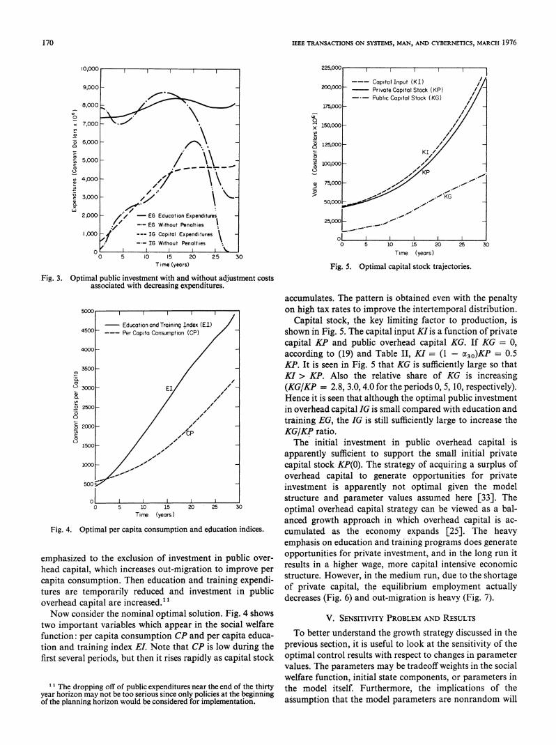
accumulates. The pattern is obtained even with the penalty5000 on high tax rates to improve the intertemporal distribution.

- EuainadTiigndxCapital stock, the key limiting factor to production, is450-

Education and Training Index (EI)4500 Per Capita Consumption (CP) shown in Fig. 5. The capital input KI is a function of private

capital KP and public overhead capital KG. If KG = 0,4000 _ / _ according to (19) and Table II, KI = (1 - OC30)KP = 0.53500 - KP. It is seen in Fig. 5 that KG is sufficiently large so that

Kl > KP. Also the relative share of KG is increasingo 3000 El (KG/KP = 2.8, 3.0, 4.0 for the periods 0, 5, 10, respectively).CL | / ' | Hence it is seen that although the optimal public investmenta250027 _ in overhead capital IG is small compared with education and

o 2000L / ,, j training EG, the IG is still sufficiently large to increase the2000-X ACP KG/KP ratio.

The initial investment in public overhead capital isapparently sufficient to support the small initial private

ooow / ,capital stock KP(O). The strategy of acquiring a surplus ofoverhead capital to generate opportunities for private

500 investment is apparently not optimal given the model

0 1 2 structure and parameter values assumed here [33]. TheT5 10 15 20 25 30 optimal overhead capital strategy can be viewed as a bal-

anced growth approach in which overhead capital is ac-Fig. 4. Optimal per capita consumption and education indices. cumulated as the economy expands [25]. The heavy

emphasis on education and training programs does generateopportunities for private investment, and in the long run itemphasized to the exclusion of investment in public over- oresults in a higher wage, more capital intensive economichead capital, which increases out-migration to improve per r

capita consumption. The education and training ep structure. However, in the medium run, due to the shortagecapita consumption. Then education and training expendi-*tures are temporaril reduc and inof private capital, the equilibrium employment actuallytures are temporarily reduced and investment in pUbliC

overhead capital are increased." decreases (Fig. 6) and out-migration is heavy (Fig. 7).Now consider the nominal optimal solution. Fig. 4 shows

two important variables which appear in the social welfare V ESTVT RBE N EUTfunction: per capita consumption CP and per capita educa- To better understand the growth strategy discussed in thetion and training index EI. Note that CF is low during the previous section, it is useful to look at the sensitivity of thefirst several periods, but then it rises rapidly as capital stock optimal control results with respect to changes in parameter

values. The parameters may be tradeoffweights in the socialwelfare function, initial state components, or parameters in

'1 The dropping off of public expenditures near the end of the thirty the model itself. Furthermore, the implications of theyear horizon may not be too serious since only policies at the beginning.of the planning horizon would be considered for implementation. assumption that the model parameters are nonrandom will


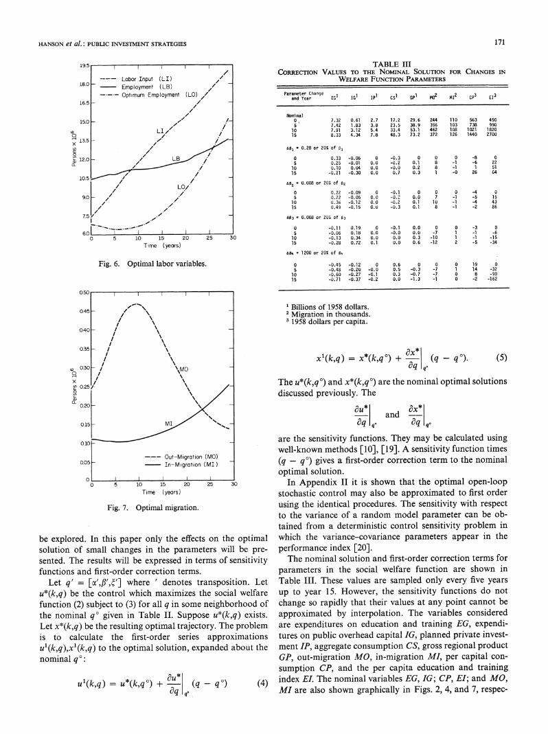
19.5 TABLE III/ CORRECTION VALUES TO THE NOMINAL SOLUTION FOR CHANGES IN

Labor Input (LI) So WELFARE FUNCTION PARAMETERS18.0 - Employment (LB)

Optimum Employment (LO) / Parameter Change I I I I 1 2 2 3 3/ ~~~~~~~~~~~~andYear EG G I C1M M P E

16.5/ 14oneinal

15.0_-' 0, 7.32 0.61 2.7 17.2 29.6 244 110 563 450/ 5 7.42 1.83 3.8 23.5 38.9 396 103 738 990

aD LI/o 18 7.91 3.12 5.4 33.4 53.1 462 108 1021 1820O / 8/15 8.33 4.34 7.8 48.3 73.2 372 126 1440 2780X 13.5

c / BI. 08) 8.28 or 201 of al

12.0 - LB 8 0.33 -0.06 0 -0.3 0 0 0 -8 0aC.L/ / 5 8.25 -0.01 0.0 -0.2 0.1 8 -1 -6 22

/ * 10 010 0.04 0.8 -0.0 0.2 8 -1 1 51

10.57 ./ _

15 -0.21 -0.30 0.0 0.7 0.3 1 -0 26 64

/ LO/ 882 8.008 or 20% of 020 0.22 -0.09 0 -8.1 0 0 0 -4 0

9.0 ./ 5 0.22 -0.05 0.0 -0.2 0.0 7 -1 -5 15,/. 180 0.36 -0.12 0.0 -0.2 0.1 10 -1 -4 43

15 0.49 -0.15 8.0 -0.3 0.1 8 -1 -2 86

7.5/ 0A3 = 0.008 or 20% of 83

| _ _._ ~ ~ ~~~~~~~~~~~~~~~~~~~~~~~~0-0.110.190 -O.1I 0.0 0 0 -3 06.0 5 -0. 06 0.182 0.0 -0. 0 0.0 --7 1 1 -6

a 5 1O 15 20 25 30 lo -0.13 0.34 0.0 0.0 0.3 -10 1 -1 -15

Time (years) 15 -0.28 0.72 0.1 0.0 0.6 -12 2 -5 -34604 1200 or 201 of BE

Fig. 6. Optimal labor variables. 8 -0.45 -0.12 0 0.6 0 0 0 19 05 -0.48 -0.20 -0.0 0.5 -0.3 -7 1 14 -32

1 0 -0.60 -0.27 -0. 1 0.3 -0.7 -7 0 8 -901 5 -0. 71 -0.37 -0.2 0.0 -1.3 -1 0 -2 -162

0.506

Billions of 1958 dollars.0.45 2 Migration in thousands.3 1958 dollars per capita.

0.40

x'(k,q) = x*(k,q°) + (q q (5)0.30 MO 1oq q

x 0.2s / \ - The u*(k,q°) and x*(k,q°) are the nominal optimal solutionsdiscussed previously. The

0.20 3 n -and

0.15 5 /Oq q= Oqqq

0.10 _are the sensitivity functions. They may be calculated usingwell-known methods [10], [19]. A sensitivity function times

0.05 uIn-Migration (MI) (q -qq) gives a first-order correction term to the nominal

I optimal solution.5 10 15 20 25 30 In Appendix II it is shown that the optimal open-loop

Time (years) stochastic control may also be approximated to first order

Fig. 7. Optimal migration. using the identical procedures. The sensitivity with respectto the variance of a random model parameter can be ob-tained from a deterministic control sensitivity problem in

be explored. In this paper only the effects on the optimal which the variance-covariance parameters appear in thesolution of small changes in the parameters will be pre- performance index [20].sented. The results will be expressed in terms of sensitivity The nominal solution and first-order correction terms forfunctions and first-order correction terms. parameters in the social welfare function are shown in

Let q' = [c',fl',S'] where ' denotes transposition. Let Table III. These values are sampled only every five yearsu*(k,q) be the control which maximizes the social welfare up to year 15. However, the sensitivity functions do not

function (2) subject to (3) for all q in some neighborhood of change so rapidly that their values at any point cannot bethe nominal q° given in Table II. Suppose u*(k,q) exists. .approximated by interpolation. The variables consideredLet x*(k,q) be the resulting optimal trajectory. The problem .are expenditures on education and training EG, expendi-is to calculate the first-order series approximations .tures on public overhead capital IG, planned private invest-ut(k,q),x'(k,q) to the optimal solution, expanded about the .ment IP, aggregate consumption CS, gross regional productnominal q°: .GP, out-migration MO, in-migration MI, per capital con-

sumption CP, and the per capita education and training

u'(k,q) = u*(k,q 0) + -U q0qq) (4) index El. The nominal variables EG, IG; CP, El; and MO,aqIqo ~~~~MIare also shown graphically in Figs. 2, 4, and 7, respec-


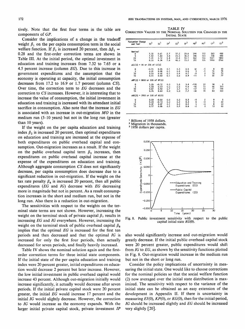
tively. Note that the first four terms in the table are TABLE IVCORRECTION VALUES TO THE NOMINAL SOLUTION FOR CHANGES IN THE

components of GP. INITIAL STATEConsider the implications of a change in the tradeoff ---

weight l,B on the per capita consumption term in the social ParaerEGIChangeIGI CS1 GP1 MO2 MI2 CP3 El3welfare function. If /3l is increased 20 percent, then Afl1 = Nominal0.28 and the first-order correction terms are shown in 0 7.32 0:61 2:7 17:2 2986 244 110 563 450

Table III. At the initial period, the optimal investment in 0 7833 4 33848 531 462 108 1021 1820education and training increases from 7.32 to 7.65 or a AEI(o) = 90 or 20% of El(0)4.5 percent increase (column EG). Due to this increase in o -0.15 0.26 0.1 0.3 0.5 32 -5 8 90

S U.01 0.08 0.1 0.4 0.6 9 -1 14 74government expenditures and the assumption that the 10 0.1 2 0.1 0.4 0.7 -9 0 18 70

15 0.11 0.03 0.1 0.6 0.9 -11 1 22 77economy is operating at capacity, the initial consumption oKP(0) = 8600 or 201 of KP(0)decreases from 17.2 to 16.9 or 1.7 percent (column CS). 0 1.26 -0.12 0.3 1.8 3.4 -100 22 58 9Over time, the correction term to EG decreases and the 10 0.87 0:49 7 3.7 6:1 -57 13 77 198correction to CS increases. However, it is interesting that to l5 0.76 0.63o .9 5.0 7.7 -32 14 83 260

increase the value of consumption, the initial investment in 0 0.50 050 0.0 0 0.3 -9 2 9Geducation and training is increased with its attendant initial ,5 0207 -0.7 0.0 0.3 0:4 5 -0 8 53sacrifice in consumption. Also note that the increase in EG 15 0.17 0.06 0.1 0.4 0.6 -2 0 13 60is associated with an increase in out-migration MO in themedium run (5-10 years) but not in the long run (greater

I of 1958 dollars.than 10 years). 2 Migration in thousands.

If the weight on the per capita education and training 3 1958 dollars per capita.index f2 is increased 20 percent, then optimal expenditureson education and training are increased at the expense ofboth expenditures on public overhead capital and con- 0.200sumption. Out-migration increases as a result. If the weighton the public overhead capital term fl3 increases, then 0.150expenditures on public overhead capital increase at the D 0.100expense of the expenditures on education and training. "Although aggregate consumption CS does not significantly "E 0.050decrease, per capita consumption does decrease due to a "zsignificant reduction in out-migration. If the weight on the co

tax rate penalty ,B4 iS increased 20 percent, then all public 2 QQ5Q _ / ---Education and Trainingexpenditures (EG and IG) decrease with EG decreasing Expenditures (EG)more in magnitude but not in percent. As a result consump- --0.100 / Expendituaes (IG)tion increases in the short and medium run, but not in thelong run. Also there is a reduction in out-migration. -0.150 /The sensitivities with respect to the weights on the ter- 0.200

minal state terms are not shown. However, increasing the o 5 10 15 20 25 30

weight on the terminal stock of private capital fl7 results in Time (years), Fig. 8. Public investment sensitivity with respect to the publicincreasing EG and IG everywhere. However, increasing the capital initial state KG(O).

weight on the terminal stock of public overhead capital ,B8implies that the optimal EG is increased for the first tenperiods and then decreased and that the optimal IG is also would significantly increase and out-migration wouldincreased for only the first four periods, then actually greatly decrease. If the initial public overhead capital stockdecreased for seven periods, and finally heavily increased. were 20 percent greater, public expenditures would shift

Table IV shows the nominal solution again and the first- from IG to EG, as shown by the sensitivity functions plottedorder correction terms for three initial state components. in Fig. 8. Out-migration would increase in the medium runIf the initial state of the per capita education and training but not in the short or long run.index were 20 percent greater, initial expenditures on educa- Consider the policy implications of uncertainty in mea-tion would decrease 2 percent but later increase. However, suring the initial state. One would like to choose correctionsthe low initial investment in public overhead capital would for the nominal policies so that the social welfare functionincrease 43 percent. Although out-migration initially would (2) now averaged over the initial state distribution is max-increase significantly, it actually would decrease after seven imized. The sensitivity with respect to the variance of theperiods. If the initial private capital stock were 20 percent initial state can be obtained as an easy extension of thegreater, the initial EG would increase 17 percent and the development in Appendix II. If there is uncertainty ininitial IG would slightly decrease. However, the correction measuring EI(0), KP(0), or KG(0), then for the initial period,to IG would increase as the economy expands. With the IG should be increased slightly and EG should be increasedlarger initial private capital stock, private investment IP very slightly [201.


TABLE V 1,500,000CORRECTION VALUES TO THE NOMINAL SOLUTION FOR CHANGES IN

INVESTMENT FUNCTION PARAMETERS1,300,000 -

Parameter Clhange I 1 1 1 1 2 23and Year EG IG IP CS GP MO MI CP EI3 Education and Training

1,100,000 - Expenditures (EG)otominal - Public Capital

0 7.32 0.61 2.7 17.2 29.6 244 110 5o3 450 X 900,000 Expenditures (IG)5 7.42 1.83 3.8 23.5 38.9 396 103 738 990

10 7.91 3.12 5.4 33.4 53.1 4b2 108 1021 182015 8.33 4.34 7.a 48.3 73.2 372 126 1440 2700 '

700,000 --

a1 2.006 or 20% of a1 70U)

0 0.24 -0.08 0.1 -0.3 0 0 0 -9 05 0.26 0.05 0.3 -0. 1 0.5 -8 1 -3 1 7 a) 500,000

10 0.56 0.23 0.5 0.5 1.7 -23 3 11 50 a1 5 0.83 0.25 1.0 1.5 3.8 -40 7 33 109

A015 .002 or 20% of 0l9 a. 300,000 -

0 -0.03 0.06 0.0 -0.1 0 0 0 -3 0 Lii5 0.02 0.07 0.1 0.0 0.2 -7 1 0 -1

10 0.13 0.05 0.1 0.2 0.6 -12 2 4 1 100,000-15 0.21 0.09 0.3 0.5 1.2 -13 2 9 1

do .012 /18 -100,000 -

0 0.07 0.22 0 -0.3 0.0 0 0 -10 05 0.02 -0.02 0.0 0.0 0.0 1 -0 1 4

10 -0.01 0.01 0.0 0.0 0.0 0 -0 1 6 -300o000o_c15 -0.01 -0.01 0.0 0.0 0.1 -0 -0 2 6 0 5 10 15 20 25 30

Ti me (years)

Fig. 9. Public investment sensitivity with respect to the variance of the1Billions of 1958 dollars. investment function parameter al 8.

2 Migration in thousands.3 1958 dollars per capita.

VI. UNCERTAINTY IN THE GROWTH RATENext the sensitivity with respect to model parameters will An important consideration when planning public in-

be discussed. The sensitivity with respect to the parameters vestment designed to improve opportunities for privateaC1,04,X6,x32 which affect the region's growth rate have been investment is the fact that the amount of induced private in-discussed elsewhere [19]. The parameters (1 - a4) and a32 vestment is uncertain [33]. This uncertainty is modeled byaffect the capital stock growth rate. The parameter X6 assuming that the coefficients in the private investmentaffects productivity through technical progress. It is shownon

function are random with constant variance and covariancethat if any of these three parameters were larger, then the within each period but with covariance zero betweenregion should take a longer run perspective with moreregin shuldake loner rn pespecive ith ore periods. The first-order correction terms, when the coeffici-public investment, more emphasis on education and train- ping, and with a small initial sacrifice in consumption [19]. ent of labor quality in the private investment function isA more capital intensive, high-wage economic structure random with a standard deviation Of u18 = 0.012, are

would evolve. Corrections in the opposite direction would shown in Table V.'2 Initially both EG and IG are greater,be appropriate if the population growth rate parameter x but IG is increased by 36 percent and EG is increased by

were grae..ftepouarra 1 percent (see Fig. 9). The qualitative form of Fig. 9 can bevarile,gathen In the intil peiod public inveiste indov described as follows: in the first year public investment in

head capltal should beincreased slightly andsintmen in overhead capital and in education and training are in-headucapiti and should be increased. , inverysl creased with the greater emphasis on overhead capital[20].ethese reslsse toubeiensteato aorrelatio During years 2-5 there is some decrease in investment inin0].Theserandom

s

seqen to populaenstivetongr -owth arelamete overhead capital. After the fifth year the stochastlc correc-

[20n tion terms are insignificant. The correction terms under thea p f assumption that the coefficient of overhead capital is ran-

thetiplanne pariate i es ion.a Table V shos th dom in the private investment function are qualitatively thethe planned private investment function. Table V shows the saebtlsinmgtu .Asosuigththerdmnominal solution and first-order correction terms for changes saefbutls in magnitud alsoassumiongac th tra min th.aaeesx8adx9 h ofiinso ao coefficients are correlated adds additional correction termsin the parameters 0Cl8 and cxlg the coefficients of labor oftesmqulaivfr.* . ' . ..~~~ith of the same qualitative form.quality and overhead capital, respectively, n the private q. .investment function. If the g18 were 20 percent greater, then is is th atinvestro ing rubis wouldead ptoaninitially public investment would shift from overhead capital sincreasein th initallin t in.publicnoverhad capita ,to education and training to take advantage of the greater s o i i i i

coefficient of labor quality in the investment function. A.so major argument against the strategy of acquiring surplusinitial Consumptionwould be sacrificed for longer-term overhead capital to generate opportunities for privatebenefits. That is, in the medium and long run EG, IG, IP,and CS all would increase. With the increase in private in- 012 Wh~en it is assumed that a model parameter is random, there are twovestment, out-migration would also decrease. The same sources which generate perturbations of the system variables about

' ~~~~~~~~~~~~~~~theirnominal traJectories: changes in the control and the random inputpattern is observed if oc,9 were greater except that initially itself. Only the first source is considered here. No attempt is made tothere would be a shift from public investment in education present the distribution of the system variables. The response to the

overheadcapital. ~~~~~~~~control correction may be close to the mean of this distribution, butto oehacaia.in general it is not exactly the mean, since the system is nonlinear.


investment is that the induced private investment, and hence head capital should be decreased. If there is uncertainty inthe benefits derived from the overhead capital, is uncertain the growth rate, then a small amount of planned future[33]. public investment in overhead capital is shifted to theHowever, the stochastic correction terms are not large present.

enough to lead to this alternative development strategy. These policy results are intended to hold for the U.S.Public investment in infrastructure is not increased to the Southeast region of 1940 and similar regions. However, thepoint where there is a significant possibility that "over validity of the arguments leading to these recommendationsinvestment" in overhead capital would occur. The qualita- is based on the accuracy of the regional model and thetive form of the stochastic corrections might be interpreted appropriateness of the social welfare function.as follows: the increase in initial investment in overhead It should also be mentioned that for the open-loopcapital has large benefits since overhead capital is scarce, but stochastic control strategy, the stochastic correction termsit also has a large opportunity cost. The opportunity cost are very small after the initial periods. This may be expected,of public investment is the value of consumption foregone since no feedback is assumed to be available. However, ato finance the public investment where the value of con- region as it develops has the option to update its develop-sumption is determined by the social welfare function. ment plans based on feedback information [14]. Then theDecreasing marginal welfare from consumption (see (1)) stochastic correction terms may again be significant. Alsoimplies that initially when consumption is low, the value of the region may correct its policies due to its actual growthconsumption is high. It also implies that a risk adverse deviating from the nominal growth trajectory and due tostrategy is optimal. improved parameter estimates [20].The opportunity cost of increasing initial public invest-

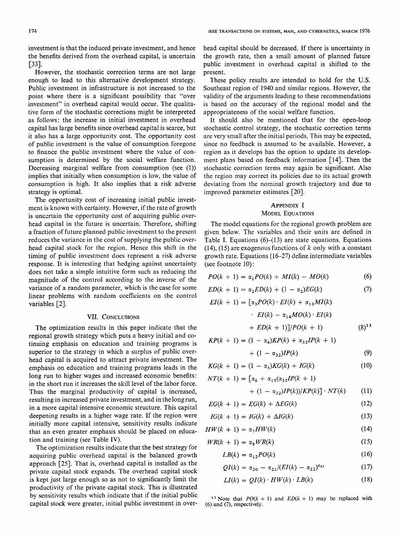
ment is known with certainty. However, if the rate of growth MODEL EQUATIONSis unc-rtain the opportunity cost of acquiring public over-head capital in the future is uncertain. Therefore, shifting The model equations for the regional growth problem area fraction of future planned public investment to the present given below. The variables and their units are defined inreduces the variance in the cost of supplying the public over- Table I. Equations (6)-(13) are state equations. Equationshead capital stock for the region. Hence this shift in the (14), (15) are exogenous functions of k only with a constanttiming of public investment does represent a risk adverse growth rate. Equations (16-27) define intermediate variablesresponse. It is interesting that hedging against uncertainty (see footnote 10):does not take a simple intuitive form such as reducing themagnitude of the control according to the inverse of the PO(k + 1) = axPO(k) + MI(k)-MO(k) (6)variance of a random parameter, which is the case for some ED(k + 1) = X2ED(k) + (1 - C2)EG(k) (7)linear problems with random coefficients on the controlvariables [2]. EI(k + 1) = [c3PO(k) * EI(k) ± c*3M1(k)

VII. CONCLUSIONS EI(k) -a14MO(k) El(k)

The optimization results in this paper indicate that the + ED(k + l)]/PO(k + 1) (8)13regional growth strategy which puts a heavy initial and co-tinuing emphasis on education and training programs is KP(k ± 1) = (1-x4)KP(k) + 32IP(k + 1)superior to the strategy in which a surplus of public over- + (1 - L32)IP(k) (9)head capital is acquired to attract private investment. Theemphasis on education and training programs leads in the KG(k + 1) = (1-x5)KG(k) ± IG(k) (10)long run to higher wages and increased economic benefits: NT(k + 1) = [:6 + a15( 32IP(k + 1)in the short run it increases the skill level of the labor force.Thus the marginal productivity of capital is increased, + (1 - C32)IP(k))/KP(k)] * NT(k) (11)resulting in increased private investment, and in the long run, EG(k 1) EG(k) EG(k) (12)in a more capital intensive economic structure. This capitaldeepening results in a higher wage rate. If the region were IG(k + 1) = IG(k) + AIG(k) (13)initially more capital intensive, sensitivity results indicatethat an even greater emphasis should be placed on educa- HW(k + 1) = x7HW(k) (14)tion and training (see Table IV). WR(k + 1) = a8WR(k) (15)The optimization results indicate that the best strategy for

acquiring public overhead capital is the balanced growth LB(k) = ca12PO(k) (16)approach [25]. That is, overhead capital is installed as theQlk= 2-z/E()x )2317private capital stock expands. The overhead capital stock Q()=~O-x1(Ik 2)(7is kept just large enough so as not to significantly limit the LI(k) = QI(k) * HW(k) * LB(k) (18)productivity of the private capital stock. This is illustratedby sensitivity results which indicate that if the initial public ' NtthtP(+1)adEk+1)mybrelcdwhcapital stock were greater, initial public investment in over- (6) and (7), respectively.


(1_-_29)KG(k) 29KP( with fixed initial state x(0). Denote by U0 the deterministicKI(k) - -I-~a3+ a30 L 29KP(k) j | K) control which maximizes (32) subject to (33). Suppose U0

(19) exists. Then expand V to third order in ((D, U) about ((F, U0),take the expectation, and drop terms which are constant or

GP(k) = c31NT(k) * [(LI(k)kL1oY~ 9higher than second order in U. The result is the following:

+ (KI(k)/ca1 )-`9]-1/a9 (20) N-1I = S(x(N)) + Y, Lk(g(k),u(k)) + Kk(B)(u(k) - u0(k))

LO(k) = [QI(k) HW(k) WR(k)) k/ = 0LO(k)= ~NT(k) v(k) ) (34)

1/ag where- v(k)J KI(k)/lxll (21) = d [d d2V]

where i= _ b1 dUk LO OJk/QI(k) HW(k)\ -9 Formulas for the total derivatives in (35) are given else-

v(k)= c10 where along with a discussion of implementation [20].Let L(B) be the control which maximizes (34) subject

IP(k) = [c17 + cc18QI(k) + c9 [KG(k)] GP(k) to (35). Then it can be shown that under fairly general[KP(k)J

G

sufficient conditions

(22) ulTR(k) = c16 + (EG(k) + IG(k))/GP(k) (23) 1bij1B=oCS(k) = (1 -ac16)GP(k) - IP(k) - EG(k) - IG(k) equals the first-order sensitivity function for the optimal

(24) open-loop stochastic control [20]. Hence to find this sensi-tivity function is to solve the problem as stated. Con-

CP(k) = CS(k)/PO(k) (25) veniently,MO(k) = cc25PO(k) + cc26QI(k) Ue-24(LO(k)LB(k))

(26) Obij B=oMI(k) = a27PO(k) + c28(LO(k) - LB(k)) (27) can be calculated using the well-known optimal control

APPENDIX II sensitivity methods used to generate all the sensitivitySTOCHASTIC CONTROL ALGORITHM information in this paper, since bij enters simply as a

parameter in the performance index (34) of a deterministicConsider a discrete-time stochastic system optimal control problem [10], [19]. This technique for

x(k + 1) = fk(x(k),u(k),b(k)) (28) approximating an optimal stochastic control seems to besimpler than the technique by Kushner based on the

with fixed initial state x(0). For some fixed terminal period stochastic maximum principle and requiring that theN, let stochastic state and costate be expanded to second order in

U = [u'(0), *,u'(N - 1)]' (29) the random vector (D [26].X = [x'(0), ,x'(N)]' (30) REFERENCES(F = [0b'(0), ,'(N - 1)]' (31) [1] R. G. D. Allen, Macroeconomic Theory. London: Macmillan,

1967.where ' denotes transposition and (F is an r-dimensional [2] M. Aoki, Optimization of Stochastic Systems. New York:

Academic, 1967.random vector with mean if, variance-covariance matrix B [3] K. J. Arrow and M. Kurz, Putblic Investment, The Rate of Return,and ith element Oi. The social welfare function is in the form and Optimal Fiscal Policy. Baltimore, Md.: Johns HopkinsPress, 1970, pp. 10-14.

N-1 [4] K. J. Arrow et al., "Capital-labor substitution and economicV(X(D,U)U) = S(x(N)) + 1 Lk(x(k),u(k)). (32) efficiency," Rev. Econ. Stat., vol. 43, pp. 225-250, Aug. 1961.V(X=((F, U), ) G. H. Borts, "The estimation of produced income by state and

k 0 region," in The Behavior of Income Shares, Studies in Income

Some differentiability properties are needed onfk, Lk, and and Wealth, NBER, vol. 27. Princeton, N.J.: Princeton Univ.Press, 1964, pp. 317-381.

S [20, pp. 69-70]. The optimal open-loop stochastic control [6] S. Bowles, "Migration as investment: Empirical tests of the humanis the sequence U which maximizes the expected value of Stat-,.investment approach to geographical mobility," Rev. Econ.(32) subject to (28). Assume that this control exists and that [7] A. B. Bryson and Y. C. Ho, Applied Optimal Control. Walthamit is continuously differentiable. The problem is to find a [8] Mas.:Blaisdell, 1969. petpliisfr oten tl,first-order approximation to the optimal open-loop stoch- Quart. .J. Econ., vol. 76, pp. 515-547, Nov. 1962.

astic control. ~~~~~~~~~[9]S. Chakravarty, Capital and Development Planning. Cambridge,as 1C con ro . _ ~~~~~~~~~~Mass.:M.I.T., 1969.For (F equal to the nonrandom (F, the deterministic state [10] J.-B. Cruz, Jr., Feedback Systems. New York: McGraw-Hill,

x(k) will begivenby [11] ~~~~E.F. Denison, The Sources of Economic Growth in the Unitedx(k + ) =fkx(k),uk),$(k) (33) States. New York: Committee for Economic Development,

176 IEEE TRANSACTIONS ON SYSTEMS, MAN, AND CYBERNETICS, VOL. SMC-6, NO. 3, MARCH 1976

[12] A. K. Dixit, "Optimal development in the labour-surplus econ- [25] A. 0. Hirschman, The Strategy of Economic Development. Newomy," Rev. Econ. Stud., vol. XXXV, pp. 23-34, Jan. 1968. Haven, Conn.: Yale Univ. Press, 1958.

[13] A. R. Dobell, "Some characteristic features of optimal control [26] H. J. Kushner, "Near optimal control in the presence of smallproblems in economic theory," IEEE Trans. Automat. Contr., stochastic perturbations," J. Basic Eng., vol. 87, Series D., pp.vol. AC-14, pp. 39-49, Feb. 1969. 103-180, Mar. 1965.

[141 S. E. Dreyfus, "Introduction to stochastic optimization and [27] K. J. Lancaster, "A new approach to consumer theory," J. Polit.control," in Stochastic Optimization and Control, H. F. Karreman, Econ., vol. 74, pp. 132-157, Apr. 1966.Ed. New York: Wiley, 1968, ch. 1. [28] I. S. Lowry, Migration and Metropolitan Growth: Two Analytical

[15] J. S. Floyd, "Trends in southern money, income, savings, and Models. San Francisco: Chandler, 1966.investment," The South in Continuity and Change, J. C. McKinney [29] J. G. Maddox, The Advancing South: Manpower Prospects andand E. T. Thompson, Eds. Durham, N.C.: Duke Univ. Press, Problems. New York: Twentieth Century, 1967.1965, pp. 132-144. [30] N. Newman, The Political Economy of Appalachia. Lexington,

[16] J. Friedmann, Regional Development Policy: A Case Study of Ky.: Heath, 1972.Venezuela. Cambridge, Mass.: M.I.T. Press, 1966. [31] H. W. Richardson, Urban Economics. Harmondsworth, England:

[17] C. H. Hamilton, "Continuity and change in southern migration," Penguin, 1971, pp. 92-102.The South in Continuity and Change, J. C. McKinney and E. T. [32] J. Riew, "Migration and public policy," J. Regional Sci., vol. 13,Thompson, Eds. Durham, N.C.: Duke Univ. Press, 1965, pp. pp. 65-76, Apr. 1973.53-78. [33] P. N. Rosenstein-Rodan, "How to industrialize an under-

[18] N. M. Hansen, Rural Poverty and the Urban Crisis. Bloomington, developed area," Regional Economic Planning, W. Isard, Ed.Ind.: Indiana Univ. Press, 1970. Paris: Organization for Economic Co-operation and Develop-

[19] D. A. Hanson, J. B. Cruz, Jr., and W. R. Perkins, "Near optimal ment, 1961, ch. 9.regional investment using a simultaneous equation economic [34] N. Sakashita, "Regional allocation of public investment," Papersmodel," Automatica, vol. 10, pp. 595-605, Nov. 1974. Regional Sci. Ass., vol. 19, pp. 161-182, 1967.

[20] D. A. Hanson, "Optimally sensitive stochastic control with [35] L. A. Sjaastad, "The costs and returns of human migration,"regional development planning applications," Coordinated J. Polit. Econ., vol. 60, pp. 80-93, Oct. 1962.Science Lab., Univ. of Illinois, Urbana, Rep. T-7, Jan 1973. [36] W. J. Stober, "Employment and economic growth: Southeast,"

[21] D. A. Hanson, W. R. Perkins, and J. B. Cruz, Jr., "A simulation Monthly Labor Rev., vol. 91, pp. 22-23, Mar. 1968.study of regional development strategies," in Socio-Economic [37] R. M. Solow, "Technical change and the aggregate productionSystems and Principles. Pittsburgh, Pa.: Univ. of Pittsburgh, function," Rev. Econ. Stat., vol. 39, pp. 312-320, Aug. 1957.1973, ch. 5.2. [38] A. Takayama, "Regional allocation of investment: A further

[22] D. A. Hanson, "Modeling political penalties for regional develop- analysis," Quarterly J. Econ., vol. 18, pp. 330-337, May 1967.ment planning," in Proc. 4th Ann. Pittsbur.gh Conf. Modeling and [39] W. R. Thompson, A Preface to Urban Economics. Baltimore,Simulation. Pittsburgh, Pa.: Univ. of Pittsburgh, 1973, pp. Md.: Johns Hopkins Press, 1968.435-439. [40] B. A. Weisbrod, External Benefits ofPublic Education. Princeton,

[23] J. M. Henderson and R. E. Quandt, Microeconomic Theory. N.J.: Princeton Univ. Press, 1964.New York: McGraw-Hill, 1971. [41] A. R. Winger, "Supply oriented urban economic models,"

[24] B. G. Hickman, Ed., Quantitative Planning of Economic Policy. Amer. Inst. Planners J., vol. 35, pp. 30-34, Jan. 1969.Washington, D.C.: Brookings Inst., 1965, chs. 1, 5, 11.

Identification of Parameters in a FreewayTraffic Model

MOHINDER S. GREWAL, MEMBER, IEEE, AND HAROLD J. PAYNE, MEMBER, IEEE

Abstract-The methodology of discrete time, extended Kalman real freeway traffic data, especially as can be obtained from automatedfiltering is applied to the problem of identifying parameters of a macro- surveillance systems, are discussed.scopic freeway traffic model. Macroscopic models provide a representa-tion of traffic flow in terms of its gross properties, i.e., volume, density, I. INTRODUCTIONand speed. The local identifiability of a parameterization of macroscopicmodel at nominal values of the unknown parameters is checked before AUTOMATIC freeway surveillance and control systemsany identification is attempted. It is shown that the parameterization is /A have been introduced in several cities over the last tenlocally identifiable. Two parameters of the model (reaction time and years. The ultimate objective of the surveillance and controlsensitivity to changing density) were identified through the use of this systems is to achieve improved traffic movement throughmethodology.The data base for studies to date was generated from a microscopic various control techniques [1]. The difficulty in applying

simulation of freeway traffic, which involves following all individual modern or conventional control theory to traffic controlvehicle movements. Techniques for extending the methodology to employ lies mainly in the lack of adequate models of the freeway

systems. Such models would help in the understanding ofManuscript received April 7, 1975; revised October 10, 1975. This congestion and in establishing the basis for developing

work was supported in part by the National Science Foundation under traffic responsive control schemes [2]. Metering traffic

M. S. Grewal is with Division of Engineering, California State entering freeway on-ramps as a function of gross features ofUniversity, Fullerton, CA 92634. traffic, i.e., volume, density, and mean speed, has beenH. J. Payne is with Technology Service Corporation, Los Angeles, fon to be anefciemasooto. Marocoi

CA. ''fudt ea fetv en fcnrl arsol

public investment strategies for regional development: an analysis based on optimization and...

Documents