Varieties of information visualization

Michael Friendly Psych 6135

http://euclid.psych.yorku.ca/www/psy6135 @datvisFriendly

So many types

2

There are so many kinds of charts, diagrams, graphs, maps What are their features? What tasks are they good for? – Accuracy or speed of judgment? Memorability?

Topics • Statistical data graphs 1D: dotplot, boxplot, violin plot 1.5D: time-series plot, density plot, bar chart, pie

chart 2D: scatterplot, ridgeline plot 3D: contour plot, 3D scatterplot, surface plot

• Thematic maps Choropleth map Anamorphic map Flow maps

• Network & tree visualization • Animation & interactive graphics

3

1D: Infographic vs. Data graphic

4

The same data can be shown in different forms, for different purposes

One might argue that this infographic has greater impact in showing the relative size of GDP

One might argue that this statistical graph makes comparisons easier

1D: Dotplots & boxplots

5

Boxplots summarize the important characteristics of a univariate data distribution: • center (median) • spread (IQR) • shape (symmetric? skewed?) • outliers?

25% 75% M

IQR

outliers

This example overlays the boxplot with a jittered dotplot, so we can also see the individual observations

This visualization made the longlist for the 2015 Kantar Information is beautiful award. Data & R code: https://github.com/zonination/perceptions

What number do you give to a probability phrase?

1D: Density ridgeline plots

6

Another possible 1D display is a density estimate– a statistically smoothed histogram.

For comparing a set of them, a ridgeline plot stacks them vertically to create the impression of a mountain range.

As in the boxplot version, this uses:

• a progressive scale of colors • transparent colors to handle overlap Q: What features stand out here?

Software note: These figures are drawn with R, using ggplot2 and the ggridges package. See: https://cran.r-project.org/web/packages/ggridges/vignettes/introduction.html

1.5D: Time series line graphs

7

William Playfair (1786), The Commercial and Political Atlas, invented the time series line graph as a way to show data on England’s trade with other countries

One curve for imports, one for exports The balance of trade could be seen as the difference between the curves Trade with Germany was consistently in favor of England With North America, the balance changed back and forth over time Economic ‘history’ could now be visualized and explained

Psychology: Distances between curves

8

What Playfair didn’t know is that judgments of distance between curves are biased We tend to see the perpendicular distance rather than the vertical distance

where did this spike come

from?

Plotting balance of trade directly

Time series graphs

9

Things get messy when there are many series to be compared To be fair, this was designed as timeline of history– a visual story of economics. It was Playfair’s last graph.

Playfair, W. (1824) Chronology of Public Events and Remarkable Occurrences.

Parallel ranked list charts

10

Another solution for multiple time series is to chart the ranks of observations and connect them with lines to show changes in relative position.

From: Statistical Atlas of the United States (1880)

Slopes of lines reflect change in rank Red bars try to show the numbers

2D: Scatterplots: Ford Nation

11

Who voted for Rob Ford in the 2014 Toronto mayoral election?

These simple scatterplots by data journalist Patrick Cain use simple enhancements: • Color, for candidate (Chow, Ford, Tory) • Overall regression line

Source: https://globalnews.ca/news/1652571/ford-nation-2014-15-things-demographics-tell-us-about-toronto-voters/

income % immigrants

Scatterplots: Wage gap

12 Alberto Cairo, The Truthful Art, Fig 9.19, from: http://www.nytimes.com/interactive/2009/03/01/business/20090301_WageGap.html

How to compare salaries of men & women in different occupations? The NYT chose to plot median salaries for women against those for men, in different occupational groups The 45o line represents wage parity Other lines show 10, 20, 30% less for women

Scatterplots: InfoVis

13

This graph, from fivethirtyeight.com was designed to show how some presidential candidates had shifted positions before the 2016 election. The axes are a score on social and economic policy, but they rotate the axes by 45o to create zones related to political thought. This info graphic is eye-catching and self-explanatory: • colored/labeled zones • interpretive labels on axes • arrows showing movement to

extremes

14

Scatterplots: Annotations enhance perception

Data from the US draft lottery, 1970

• Birth dates were drawn at random to assign a “draft priority value” (1=bad)

• Can you see any pattern or trend?

This is an example of data with a weak signal and a lot of noise

Me (May 7): 127 → priority = 35

15

Scatterplots: Smoothing enhances perception

Drawing a smooth curve shows a systematic decrease toward the end of the year.

• The smooth curve is fit by loess, a form of non-parametric regression.

Visual explanation:

Smoothing by grouping and summarization

16

Another form of smoothing is to make one variable discrete & show a graphical summary – here a boxplot The decrease in later months becomes apparent Perception: the boxplots form the foreground; the jittered points show the data

Scatterplot matrices

17

A scatterplot matrix shows the bivariate relation between all pairs of variables. Seeing these all together is more useful than a collection of separate plots.

How does occupational prestige depend on %women, education and income? The individual plots are enhanced with linear regression lines and non-parametric smooths to show non-linearity

This figure uses scatterplotMatrix() in the car package. There are many options.

Scatterplot matrices

18

Density plots are often more useful for showing the shapes of distributions • women: bimodal • income: highly skewed A data ellipse gives a visual summary of the direction and strength of the relationship Again, graphical annotation provides aids for interpretation.

Larger data sets

19 From: http://junkcharts.typepad.com/junk_charts/2010/06/the-scatterplot-matrix-a-great-tool.html

Scatterplot matrices hold up well with a larger number of variables

Where to live in NYC? This SPM shows 12 variables on ~ 60 neighborhoods The data ellipses provide a visual summary

Categorical data

20

This remarkable chart shows survival on the Titanic, by Class for passengers and Gender and Age. It was drawn by G. Bron, a graphic artist, and published in The Sphere, one month after the Titanic sank. It uses back-to-back bar charts, with area ∼ frequency

See our web page: http://datavis.ca/papers/titanic/

Categorical data: Mosaic plots

21

Similar to a grouped bar chart Shows a frequency table with tiles, area ~ frequency

> data(HairEyeColor) > HEC <- margin.table(HairEyeColor, 1:2) > HEC Eye Hair Brown Blue Hazel Green Black 68 20 15 5 Brown 119 84 54 29 Red 26 17 14 14 Blond 7 94 10 16 > chisq.test(HEC) Pearson's Chi-squared test data: HEC X-squared = 140, df = 9, p-value <2e-16

How to understand the association between hair color and eye color?

Mosaic plots

22

Shade each tile in relation to the contribution to the Pearson χ2 statistic

> round(residuals(chisq.test(HEC)),2) Eye Hair Brown Blue Hazel Green Black 4.40 -3.07 -0.48 -1.95 Brown 1.23 -1.95 1.35 -0.35 Red -0.07 -1.73 0.85 2.28 Blond -5.85 7.05 -2.23 0.61

22 2 ( )ij ij

ijij

o er

eχ

−= = ∑∑

Mosaic plots extend readily to 3-way + tables They are intimately connected with loglinear models See: Friendly & Meyer (2016), Discrete Data Analysis with R, http://ddar.datavis.ca/

Parallel Sets

23

Parallel sets use parallel coordinate axes to show the relations among categorical variables.

The frequencies of one variable (Class) are sub-divided according to the joint frequencies in the next (Sex) and shown by the width of the connecting line.

The ParSets application is interactive:

• categories can be reordered (a, b) • categories can be grouped (c, d)

From: Kosera et al. (2006), https://kosara.net/papers/2006/Kosara_TVCG_2006.pdf

Titanic data: Who survived?

Sankey diagram

24

Pantheon, by Valerio Pellegrini Visualizing the 100 most influential figures in History (Wikipedia visits) Columns show occupation, country of origin and gender Flow lines link individuals to the column variables, width ~ influence

Sankey diagram

25 From: http://visualoop.com/blog/83382/pantheon-by-valerio-pellegrini

Multiple dimensions of the most influential people in history

Generalized pairs plots

26

Generalized pairs plots from the gpairs package handle both categorical (C) and quantitative (Q) variables in sensible ways

x y plot

Q Q scatterplot

C Q boxplot

Q C barcode

C C mosaic

library(gpairs) data(Arthritis) gpairs(Arthritis[, c(5, 2:5)], …)

3D: Iso-contour maps

27

Early attempts to show 3D data used contours of equal value on a map The data was actually very thin; the contours the result of imaginative smoothing

Francis Galton, Isochronic chart of travel time, 1881

3D: Bivariate density estimation

28

John Snow’s map of cholera deaths in London, 1854

Modern statistical techniques can compute contours of constant density

3D: population pyramid

29

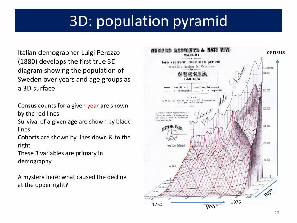
Italian demographer Luigi Perozzo (1880) develops the first true 3D diagram showing the population of Sweden over years and age groups as a 3D surface Census counts for a given year are shown by the red lines Survival of a given age are shown by black lines Cohorts are shown by lines down & to the right These 3 variables are primary in demography. A mystery here: what caused the decline at the upper right?

year 1750 1875

census

3D: scatterplot & regression surface

30

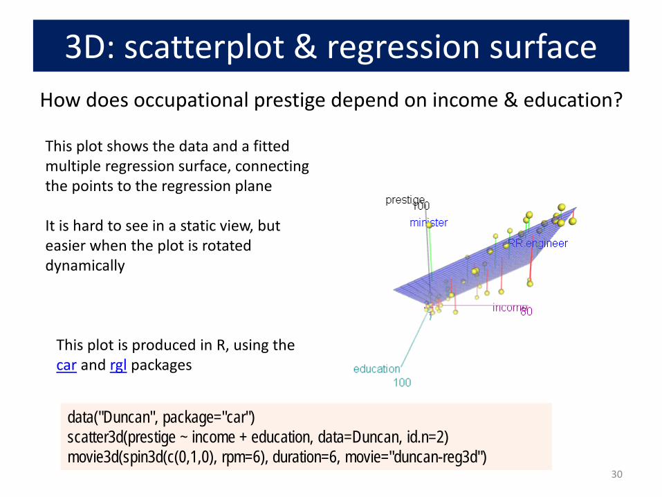
How does occupational prestige depend on income & education?

This plot shows the data and a fitted multiple regression surface, connecting the points to the regression plane It is hard to see in a static view, but easier when the plot is rotated dynamically

This plot is produced in R, using the car and rgl packages

data("Duncan", package="car") scatter3d(prestige ~ income + education, data=Duncan, id.n=2) movie3d(spin3d(c(0,1,0), rpm=6), duration=6, movie="duncan-reg3d")

Thematic maps & Spatial visualization

31

Thematic maps use a wide variety of techniques to display quantitative or qualitative variables on the geographic framework of a map Once the domain of cartographers, these ideas are now being developed as an area of geospatial visualization and geospatial statistical methods

From: Slocum et al., Thematic cartography and geographical visualization, Fig 4.3

Thematic maps: Types

32

Basic types of thematic maps Most are direct mappings of numbers to visual variables Isopleth maps combine some analysis with display

From: Slocum et al., Thematic cartography and geographical visualization, Fig 4.9

Thematic maps: Theory

33

Alan MacEachern (1979) classifies point, line and area symbols on thematic maps according to whether they depict quantitative or qualitative phenomena, in the physical or cultural domain.

MacEachern, A. (1979). The Evolution Of Thematic Cartography / A Research Methodology and Historical Review, The Canadian Cartographer 16(1) June 1979, p. 17-33

Theories, ideas, and methods have advanced considerably since this time.

Choropleth maps

34

Balbi & Guerry (1829) • First thematic maps of crime

data • First comparative maps

(“small multiples”) • Crime against persons

inversely related to crime against property

• Education: France obscure & France éclairée

• N. of France highest in education & also property crime

Anamorphic maps • Anamorph: Deforming a

spatial size or shape to show a quantitative variable

• Émile Cheysson used this to show the decrease in travel time from Paris to anywhere in France over 200 years

35

Album de Statistique Graphique, 1888, plate 8

What’s wrong with choropleth maps?

36

Choropleth maps are misleading because size (area) of units dominates perception. This is particularly true for maps of the US & Canada. Not so for France (why?)

fivethirtyeight.com election predictions, Oct. 13, 2017

Montana looks bigger than Washington Note use of labels for small NE states

Cartogram (tilegrams)

37

A tilegram uses hexagonal tiles to make area proportional to a given variable

fivethirtyeight.com election predictions, Oct. 13, 2017

Here, the size of each state is made ~ number of electoral college votes

Now, it is easy to see the impact of states

38

Worldmapper: The world in cartograms

How to visualize social, economic, disease, … data for geographic units? worldmapper.com : cartograms: area ~ variable of interest (700+ maps)

39

Worldmapper: Carbon emissions These pages are well-designed according to data vis. Ideas: high impact graph + interpretive details & explanation

Worldmapper: Cholera deaths

40

Deaths from cholera in 2004. Territory size ~ proportion of worldwide deaths

http://www.worldmapper.org/display.php?selected=232

Spatial visualization: Analysis + maps Linguistics: Food dialect maps– visualizing how people speak

In the Cambridge Online Survey of World Englishes, Bert Vaux and Marius L. Jøhndal surveyed 11,500 people to study the ways people use English words. NC State Univ. student Joshua Katz turned the US data into shaded kernel density maps.

Take the survey: http://www.tekstlab.uio.no/cambridge_survey Programming in R: http://blog.revolutionanalytics.com/2013/06/r-and-language.html

soda vs. pop?

41

Spatial visualization: Analysis + maps Linguistics: Food dialect maps– visualizing how people speak

crawfish, crawfish, crawdad?

A k-nearest neighbor kernel density estimate over (x,y) locations gives a smoothed & interpretable display of the choice probabilities. Regional differences are quite apparent. The use of color combines discrete categories with intensity to give a meaningful display

42

43

Flow maps

• Marey (1878): “defies the pen of the historian in its brutal eloquence” • Tufte (1983): “the best statistical graphic ever produced”

Flow maps show movement or change in a geographic framework The master work is this image by Charles Joseph Minard (1869)

44

Effect of US civil war on cotton trade Before After

Note the deformation of the map to accommodate the data

The Great Migration

45

In a graphic tribute to C. J. Minard and W. E. B. Du Bois, Raymond Andrews & Howard Wainer tell the story of the migration of blacks from the southern US after freedom from slavery.

Andrews, R. J. & Wainer, H. The Great Migration: A Graphics Novel Featuring the Contributions of W. E. B. Du Bois and C. J. Minard. Significance, 2017, 14, 14-19. See also: http://infowetrust.com/picturing-the-great-migration/ for the story of this graphic

Network visualization

47

Once the domain of mathematicians & computer scientists, graph theory and network visualization turn out to have surprising & interesting applications.

From: http://www.martingrandjean.ch/connected-world-air-traffic-network/ See more: https://flowingdata.com/2016/05/31/air-transportation-network/

Animated demo by Martin Granjean showing transport of passengers from/to world airports. It illustrates the difference between geography & force-directed layout to focus on volume & connections

Network visualization: Transport maps

48

How do I get from Chigwell to Charing Cross? How much will it cost? This route map shows the connections and fare zones The first one was designed by Henry Beck in 1931. The modern version is zoomable and available on your phone.

See: https://tfl.gov.uk/maps/track

Network visualization: Shakespeare tragedies

49

A new form of literary criticism? Martin Grandjean looked at the structure of Shakespeare tragedies through character interactions.

Each circle (node) represents a character, and an edge represents two characters who appeared in the same scene.

The structural characteristics of the graphs have meaningful interpretations.

From: https://flowingdata.com/2015/12/30/shakespeare-tragedies-as-network-graphs/

Semantic memory: Cognitive structure

50

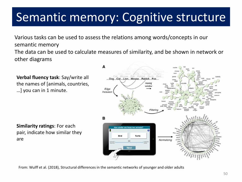
Various tasks can be used to assess the relations among words/concepts in our semantic memory The data can be used to calculate measures of similarity, and be shown in network or other diagrams

Verbal fluency task: Say/write all the names of [animals, countries, …] you can in 1 minute.

Similarity ratings: For each pair, indicate how similar they are

From: Wulff et al. (2018), Structural differences in the semantic networks of younger and older adults

Semantic memory: Cognitive structure

51

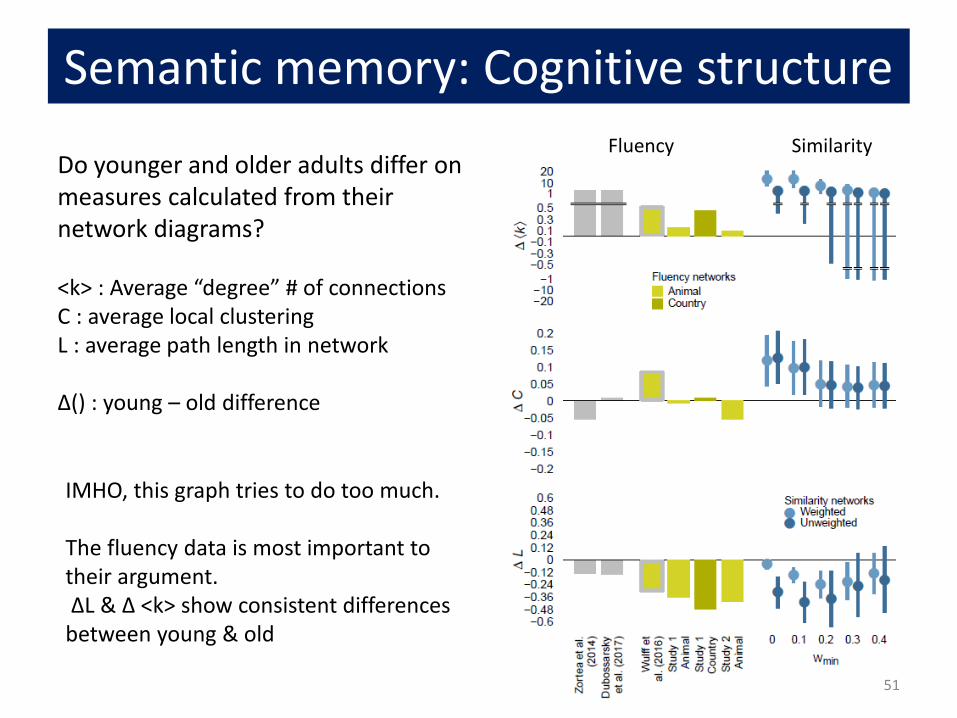
Do younger and older adults differ on measures calculated from their network diagrams? <k> : Average “degree” # of connections C : average local clustering L : average path length in network Δ() : young – old difference

Fluency Similarity

IMHO, this graph tries to do too much. The fluency data is most important to their argument. ΔL & Δ <k> show consistent differences between young & old

Love, Actually: Interactive app

52

Interactive Shiny app: https://dgrtwo.shinyapps.io/love-actually-network/

Interactions among characters in Love, Actually

Data:

WikiLeaks Iraq war logs

53

Johnathan Stray & Julian Burgess analyzed > 11,000 documents for SIGACT (“significant action”) reports from the 2006 Iraqi civil war made available by WikiLeaks.

Each report is a dot. Each dot is labelled by the three most “characteristic” words in that report.

Documents that are “similar” have edges drawn between them, width ~ similarity

The graph-drawing algorithm placed similar nodes together

From: http://jonathanstray.com/a-full-text-visualization-of-the-iraq-war-logs

WikiLeaks Iraq war logs

54

Certain themes became clear, and could be studied in rich detail The underlying methods use “term frequency–inverse document frequency” measures of text-mining.

http://jonathanstray.com/wp-content/uploads/2010/12/Murders.png

Murder cluster. All contain the word “corpse”

http://jonathanstray.com/wp-content/uploads/2010/12/Torture-abduction.png

Torture-abduction cluster

Twitter network of R users

55 From: https://perrystephenson.me/2018/09/29/the-r-twitter-network/

Perry Stephenson explores the connections among the top 50 R users on Twitter

library(rtweet) followers <- get_followers(“datavisFriendly"))

The rtweet package provides access to Twitter info

Tree diagrams

56

Trees are natural, organic visual metaphors for branching processes and space-filling designs.

Charles Darwin’s first visual sketch of the evolution of species

Ramon Llull’s tree of science, showing roots and branches of knowledge

57

History as a Tree: Geschictesbaum Europa (2003)

• The entire history of Europe in one diagram • space-filling design: resolution ~ time2

• natural metaphors for roots, branches

Image: http://euclid.psych.yorku.ca/SCS/Gallery/images/timelines/geschict1000.jpg

58

History as a Tree

• linear horizontal scale area ~ time2

• Branches for countries & domains of thought • Leaves for all the details

Treemaps

59

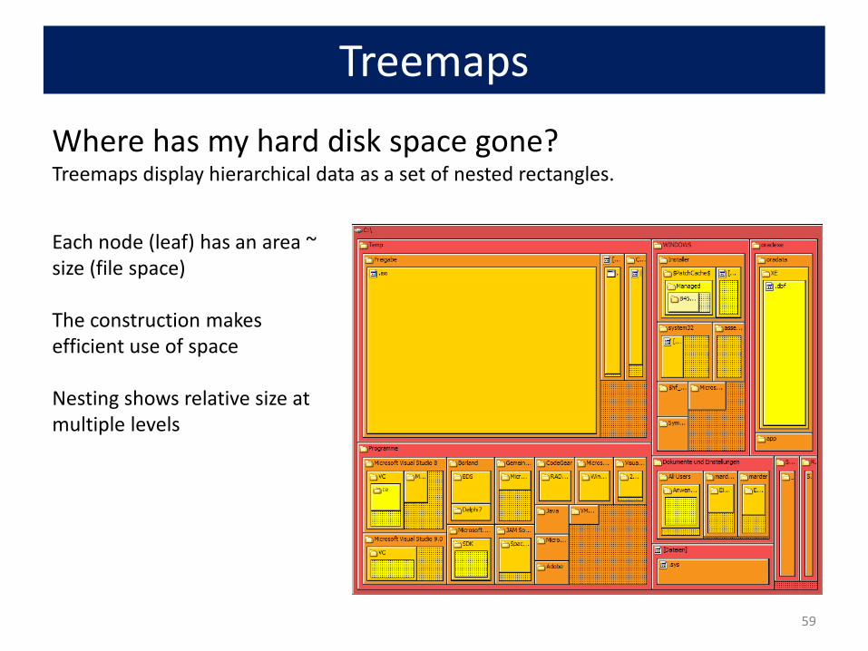
Where has my hard disk space gone? Treemaps display hierarchical data as a set of nested rectangles.

Each node (leaf) has an area ~ size (file space) The construction makes efficient use of space Nesting shows relative size at multiple levels

Treemaps: Google Newsmap

60

They turn out to be useful in a wide range of applications Google NewsMap shows top news stories with • Size ~ popularity • Color: domain– world

news, sports, national, … • Shades: recency Interactivity: Hover, click to show details

Radial trees: Visual Thesaurus

61

The Visual Thesaurus, from Thinkmap was the first application to make word meanings visual and interactive. They used a radial layout to show the various related senses of given focus word. This application was incisive in promoting ideas of interaction with tree-based data: query, zoom, tool-tips, …

This fig from Manuel Lima, The Book of Trees, p. 127

Animation & Interactive Graphics

• Origins: Visualizing motion • Animated graphics • Dynamically updated graphics • Linking views • Interactive application development frameworks

62

E.-J. Marey: A science of visualizing motion

• Physiology: How to make internal physiological processes subject to visual analysis? Invented many graphic recording devices (heart rate, blood

pressure, muscle contraction, etc.) “Every kind of observation can be expressed by graphs”

63

Marey’s sphygmograph, recording a visual trace of arterial blood pressure

Animation: Chronophotography

64

Marey pioneered the study of human and animal motion photographically

The photographic gun, allowing recording of 12 frames/sec. at intervals of 1/720 of a second

Animated graphics

65

Animated graphics, like movies are just a series of frames strung together in a sequence The data for this animation come from human figures in motion-capture suits dancing the Charleston. The Carnegie-Mellon Graphics Lab maintains a Motion Capture Database, http://mocap.cs.cmu.edu/

From: http://blog.revolutionanalytics.com/2017/08/3-d-animations-with-r.html

Statistical animations

66

Statistical concepts can often be illustrated in a dynamic plot of some process. This example illustrates the idea of least squares fitting of a regression line. As the slope of the line is varied, the right panel shows the residual sum of squares. This plot was done using the animate package in R.

Animated graphics

67

Hans Rosling captivated audiences with dynamic graphics showing changes over time in world health data

Video: Hans Rosling, “The best stats you’ve ever seen,” https://www.ted.com/talks/hans_rosling_shows_the_best_stats_you_ve_ever_seen

Animation & Interactivity

68

The Gapminder “moving bubble chart” was the vehicle. • Choose (x, y) variables • Choose bubble size

variable • Animate this over time

Liberating the X axis from time opened new vistas for data exploration Software made this available as a general tool

Dynamically updated data visualizations

69

You don’t need a weatherman to know which way the wind is blowing. The wind map app, http://hint.fm/wind/ is one of a growing number of R-based applications that harvests data from web sources, and presents a visualization

Linking animated views

70

This example links a dendrogram to a grand tour and map of the USArrests data to visualize a classification in 5 dimensions The grand tour animates a series of 2D projections of the 5D data The image is recorded as a GIF

From: Carson Sievert, https://plotly-book.cpsievert.me/linking-animated-views.html

Interactive application frameworks

71 https://walkerke.shinyapps.io/neighborhood_diversity/

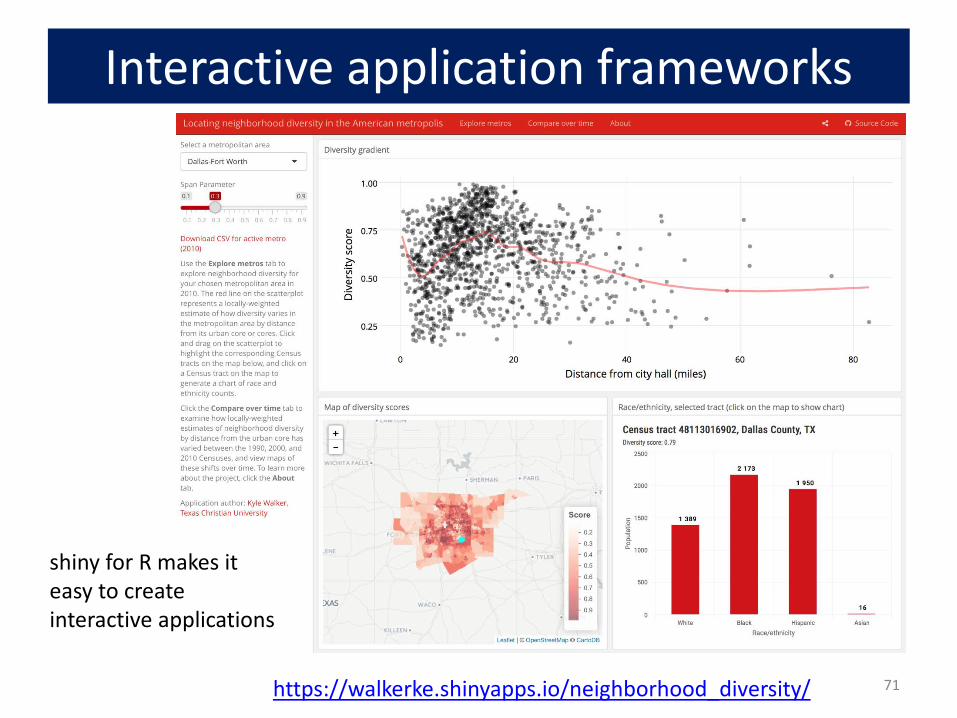
shiny for R makes it easy to create interactive applications

shiny gallery

72

There is now a large collection of shiny applications, https://shiny.rstudio.com/gallery/ These integrate other interactive web software: d3, Leaflet, Google Charts, …

Summary • The topics here were largely about data graphs, for

analysis & presentation. Mainly not Info-graphics Quantitative data: different forms for 1D, 1.5D, 2D, 3+D data Categorical data: often best shown as areas ~ frequency (bar plots,

mosaic plots)

• Thematic maps: visualizing spatially varying data Raw data with different visual encodings Spatial statistical models provide some smoothings

• Networks/trees: visualizing connections • Animation: show changes over time or space • Interaction: allow the viewer to explore the data

73