January 7, 2003 17:55

PSEUDOELASTIC SMA SPRING ELEMENTS FOR PASSIVE VIBRATIONISOLATION, PART I: MODELING

Mughees M. KhanDepartment of Aerospace Engineering

Texas A&M UniversityCollege Station, TX 77843

mkhan@tamu.edu

Dimitris C. Lagoudas∗

Department of Aerospace EngineeringTexas A&M University

College Station, TX 77843dlagoudas@aero.tamu.edu

John J. MayesV-22 Structure and Development

Airframe Systems, Bell Helicopter, TextronFort Worth, TX 76101

JJMayes@bellhelicopter.textron.com

Benjamin K. HendersonAir Force Research Laboratory/VSSV

Kirtland AFB, NM 87117benjamin.henderson@kirtland.af.mil

ABSTRACTIn this work, the effect of pseudoelastic response of shape

memory alloys (SMAs) on passive vibration isolation has beeninvestigated. This study has been conducted by developing,modeling and experimentally validating an SMA based vibra-tion isolation device. This device consists of layers of pre-constrained SMA tubes undergoing pseudoelastic transforma-tions under transverse dynamical loading. These SMA tubes arereferred to as SMA spring elements in this study. To accuratelymodel the non-linear hysteretic response of SMA tubes presentin this device, at first a Preisach model (an empirical model basedon system identification) has been adapted to represent the struc-tural response of a single SMA tube. The modified Preisachmodel has then been utilized to model the SMA based vibrationisolation device. Since this device also represents a non-linearhysteretic dynamical system, a physically based simplified SMAmodel suitable for performing extensive parametric studies onsuch dynamical systems has also been developed. Both the sim-plified SMA model and the Preisach model have been used toperform experimental correlations with the results obtained fromactual testing of the device. Based on the studies conducted it hasbeen shown that SMA based vibration isolation devices can over-come performance trade-offs inherent in typical softening spring-damper vibration isolation systems. This work is presented asa two-part paper. Part I of this study presents the modificationof the Preisach model for representing SMA pseudoelastic tuberesponse together with the implemented identification methodol-ogy. Part I also presents the development of a physically basedsimplified SMA model followed by model comparisons with theactual tube response. Part II of this work covers extensive para-

∗Corresponding author.

metric study of a pseudoelastic SMA spring-mass system usingboth models developed in part I. Part II also presents numericalsimulations of a dynamical system based on the prototype de-vice, results of actual testing of the device and correlations of theexperimental cases with the model predictions.

Keywords: Shape Memory Alloys (SMA), Pseudoelastic-ity, Hysteresis, Preisach, System Identification, Passive VibrationIsolation, Damping, Dynamic System.

NOMENCLATUREα Increasing values of displacementβ Decreasing values of displacementδ Spring displacementδA f Spring displacement denoting end of A←M

transformationδAs Spring displacement denoting start of A←M

transformationδM f Spring displacement denoting end of A→M

transformationδMs Spring displacement denoting start of A→M

transformationδtr Transformation displacementδmax Lower bound on displacementδmin Upper bound on displacementµ Weighing function in the Preisach modelσ StressA Austenite PhaseA0 f Austenite Finish temperature at zero stressA0s Austenite Start temperature at zero stress

1

f A f Force denoting end of A←M transformationf As Force denoting start of A←M transformationf M f Force denoting end of A→M transformationf Ms Force denoting start of A→M transformationf SMA Force exerted by SMA springH Hysteresis relay operatorsKA Stiffness of Austenite phaseKM Stiffness of Martensite phaseM Martensite PhaseM0 f Martensite Finish temperature at zero stressM0s Martensite Start temperature at zero stressT Temperature

1. INTRODUCTIONThe task of damping and vibration isolation is often faced

with trade-offs. The goal of vibration isolation is commonly ac-complished by using an isolation system with a relatively softerstiffness (Beranek and Ver, 1992). However, for isolation ofheavy loads, a small stiffness leads to large displacements. Thislarge displacement obstacle has often been overcome by using adevice having a nonlinear spring with decreasing stiffness, like asoftening spring. Such a device would have a stiff initial responsewhich becomes less stiff as the load is increased, so that the stiffregion of the device’s response supports the initial load and thetransmissibility is reduced by the softer stiffness of the nonlinearspring in the operating range. One of the problems encounteredin vibration isolation using a nonlinear spring is its resonant be-havior at low excitation frequencies due to softer stiffness in theoperating range. This condition results in the necessity to adddamping to the system, which has the desired effect of decreas-ing the resonant response but also degrades the response of thesystem at higher frequencies as shown by Harris (1996); Inman(2001).

To eliminate these trade-offs one can use active materials in-tegrated into smart structures. One such option is to use ShapeMemory Alloys(SMAs) as the behavior of devices with decreas-ing stiffness and a damper is similar to the hysteretic load-deflection relationship exhibited by SMAs during pseudoelasticdeformation (Otsuka and Shimizu, 1986; Wayman, 1983) as dis-cussed later.

1.1 Review of Pseudoelastic SMA Based DynamicalSystems for Damping and/or Vibration Isolation

The SMA pseudoelastic behavior is defined as inducing de-twinned martensite (M) from austenite (A) by thermomechani-cal loading, which then reverts to austenite upon removal of themechanical load. The presence of stress forces austenite to di-rectly form detwinned martensite, resulting in large macroscopicstrains, which can be fully recovered upon unloading to the zero-stress state provided the temperature is kept above a certain tem-

perature (Otsuka and Wayman, 1999; Wayman, 1983; Miyazakiet al., 1997). Figure 1 represents a schematic of a typical SMAphase diagram, showing the relationship between stress, temper-ature, and the two possible phases of the SMA. Schematic ofa typical pseudoelastic loading path as discussed above is alsoshown. The transformation temperatures at the zero-stress stateare represented as M0s,M0 f ,A0s and A0 f in Figure 1 representingmartensitic start, martensitic finish, austenitic start and austeniticfinish temperatures. In addition to the change in material prop-erties and large recoverable strain during pseudoelastic transfor-mation, there is hysteresis which is an indicator of energy dissi-pation during the forward (A→M) and reverse (M→ A) trans-formations (Figure 1b). This energy dissipation is proportionalto the degree of transformation completed during a loading cy-cle for both complete and incomplete, or partial transformations.These partial transformations are also referred to as minor loophysteresis cycles (Bo and Lagoudas, 1999b) and complete, or fulltransformations are referred to as major loop hysteresis cycles.The energy dissipation due to hysteresis provides an opportunityfor SMAs to be used as damping devices and the change in thestiffness (represented by points 1, 2, 3 and 4 in Figure 1b) of thematerial during pseudoelastic phase transformations provide op-portunities for SMAs to be used as vibration isolation devices.

Mos AosMof Aof

MartensiteAustenite

Plastic Deformation

Pseudoelastic Loading Path

a) b)Strain, ε

Str

ess,

σ

0

1

2

3

4

1

2

3

40

Stre

ss, σ

Temperature, TMos AosMof Aof

MartensiteAustenite

Plastic Deformation

Pseudoelastic Loading Path

a) b)Strain, ε

Str

ess,

σ

0

1

2

3

4

1

2

3

40

Stre

ss, σ

Temperature, T

Figure 1. a) Schematic of a typical SMA phase diagram with a typ-

ical pseudoelastic loading path noted in stress-temperature space b)

Schematic of the corresponding pseudoelastic loading path in stress-

strain space

The nature of the pseudoelastic effect, as discussed aboveand illustrated in Figure 1b, indicates the possibility of usingSMAs for vibration isolation. Utilization of SMAs for suchapplications requires understanding of the pseudoelastic nonlin-ear hysteretic response found in SMAs. Graesser and Cozzarelli(1991) introduced a model for SMA hysteretic behavior, an ex-tension of the rate independent hysteresis model introduced byOzdemir (1976) to model pseudoelastic behavior of SMAs for

2

potential structural damping and seismic isolation applications.A study on the use of SMAs for passive structural damping ispresented in Thomson et al. (1995), where three different quasi-static models of hysteresis were reviewed and compared with anexperimental investigation of a cantilevered beam constrained bytwo SMA wires. Fosdick and Ketema (1998), have consideredrate dependency by including “averaged” thermal effects in theSMA constitutive behavior. Their constitutive model is based ondynamics of single-crystal phase boundaries by Abeyaratne andKnowles (1994), and they have studied a SDOF lumped massoscillator with an SMA wire attached in parallel as a passive vi-bration damper. Seelecke (2002), in a recent publication hasconsidered both isothermal and non-isothermal SMA constitu-tive response caused by rate-dependent release and absorptionof latent heat during phase transformations by using a modi-fied version of the model presented by Achenbach and Muller(1985). In Seelecke (2002), free and forced vibrations of arigid mass suspended by a thin-walled SMA tube under torsionalloading has been considered under isothermal conditions. Fornon-isothermal conditions only free vibrations have been con-sidered and it has been shown that under a free vibration case forsuch a system, isothermal SMA constitutive response may leadto underestimation of damping and resulting forces compared toa non-isothermal SMA constitutive response.

Yiu and Regelbrugge (1995), have investigated the behav-ior of SMA springs designed to act as an on-orbit soft mountisolation system with the added benefit of precision alignmentthrough the utilization of the SMA shape memory effect. Yiuand Regelbrugge (1995) have used a physically based SMAmodel identified from an SMA helical spring response. In workdone by Feng and Li (1996), the dynamics of an SMA bar ina single degree of freedom (SDOF) spring mass damper systemis presented, where the modified plasticity model presented inGraesser and Cozzarelli (1991) is used to model the pseudoelas-tic response of an SMA bar. Key results of this work includesthat the nonlinearity due to phase transformation leads to com-plicated dynamics like period doubling cascade and chaotic mo-tion. Other results include low resonant frequency for such asystem along with a suppressed peak response. Experimental re-sults have also been presented for such a system verifying quali-tative predictions of the theory. A recent study by Lacarbonaraet al. (2001) have studied periodic and non-periodic thermome-chanical response of a shape-memory oscillator using a modifiedIvshin and Pence (1994) model and considered both isothermaland non-isothermal conditions under forced vibration and pre-sented a rich class of solutions and bifurcations including jumpphenomena, pitch fork, period doubling, complete or incompletebubble structures with a variety of non-periodic responses. Re-sults presented in Lacarbonara et al. (2001) show that for therange of parameters investigated, the non-isothermal and isother-mal response were similar to each other. Work presented byLacarbonara et al. (2001) is based on earlier work by Bernardini

and Vestroni (2002), where non-linear dynamic non-isothermalresponse of pseudoelastic shape-memory oscillators have beenpresented. Softening as well as hardening behavior is noted asthe SMA undergoes partial and full phase transformation undervarying force excitation amplitude, hysteresis shape and temper-ature. Recent work by Collet et al. (2001) have studied thebehavior of a pseudoelastic SMA (Cu-Al-Be) beam under dy-namic loading for potential vibration isolation applications usingan SMA constitutive model presented in Raniecki et al. (1992).Simulations and qualitative experimental observations presentedin Collet et al. (2001) have shown that the nonlinearity in theSMA beam response is due to the SMA undergoing phase trans-formations.

Based on the work done on SMA based dynamical systemsmentioned in the above publications there is a need to explore theeffects of SMA pseudoelasticity on vibration isolation by per-forming actual experimental correlations and conducting para-metric studies under various dynamic loading conditions on anactual SMA based vibration isolation device. In this two-part pa-per series an attempt has been made to address these issues by de-veloping, simulating, testing and performing parametric studiesand experimental correlations on a pseudoelastic SMA vibrationisolator.

1.2 SMA ModelsTo realize the goal of designing and simulating an active ma-

terial based smart structure for vibration isolation using SMAs,it is necessary to have structural models that can (a) incorporateresponse of SMAs and (b) can be used for prediction and ex-perimental correlation of dynamic response of such structures.Along with the SMA models mentioned in the previous sectionthat have been mostly used for simulating SMA based dynamicalsystems, most of the other SMA constitutive models available inthe literature do not serve this dual purpose well. Studies of otherSMA constitutive models available in the literature (Lagoudaset al., 1996; Lagoudas and Bo, 1999; Brinson, 1993; Liang andRogers, 1990; Tanaka, 1986; Patoor et al., 1987) and their uti-lization for various SMA based smart structure applications re-veal that although these models are quite accurate, they are com-putationally intensive and/or hard to implement under dynamicloading conditions.

Empirical models based on system identification (ID) havealso been used for modeling the response of different active ma-terials and one of the most popular model has been the Preisachmodel. The classical Preisach model was initially proposed inthe 1930’s by a German physicist Preisach (1935) for ferromag-netic hysteresis effects and still is the most popular hysteresismodel for ferromagnetic materials. In 1970s and 1980s a Rus-sian mathematician Krasnoselskii (Krasnoselskii and Pokrovskii,1983) examined and developed the mathematical properties ofthe Preisach model and presented the model as a spectral de-

3

composition of relay operators. As a result, a useful mathe-matical tool evolved in the form of the Preisach model whichcould model various hysteretic behaviors found in nature, with-out concern for the underlying physical mechanisms. The readeris referred to comprehensive expositions on the Preisach modelby Mayergoyz (1991), Visintin (1994) and Brokate (1994) for adetailed analysis and explanation.

The generality and the computational efficiency of thePreisach hysteresis model made it applicable to the developmentof controller designs (Hughes, 1997; Ge and Jouaneh, 1995) andstability analysis (Gorbet et al., 1997) of hysteretic ferromag-netic, ferroelectric and SMA actuators. Most of the work done todate on using the Preisach model has been focused towards ferro-magnetic and ferroelectric materials, mainly on their applicationas actuators. Recently the Preisach model has been adopted foruse in SMA applications. The suitability of the model for repre-sentation of SMA actuator hysteresis has been tested by Hughes(1997); Hughes and Wen (1994), Banks et al. (1996a,b, 1997)and Webb (1998) and work has progressed towards adaptive con-trol, stability analysis and control techniques (Gorbet et al., 1997,1998). As the Preisach model is solely concerned with systemidentification and relies on additional identification experimentsin case of any change in system conditions. Bo and Lagoudas(1999a) have correlated a thermomechanical model for SMAshape memory effect response with the Preisach hysteresis modelto avoid the need for additional identification.

However, the above work is focused on the shape memoryeffect or the actuator applications of SMAs, while work doneon pseudoelastic modeling of SMA hysteresis using the Preisachmodel is limited and only addressed in few publications. In workdone by Huo (1991), the author describes a complicated exten-sion of the Preisach model for pseudoelastic response of SMAsusing a four-parameter hysteresis operator for each SMA crys-tal. The model is compared to experimental data for an unspeci-fied polycrystalline material and the technique for identifying thecomplex model is not defined in detail and only qualitative resultsare given. Ortin (1992) has applied the classical Preisach modelto a single crystal Cu-Zn-Al SMA which has more profound hys-teresis than binary Nickel-Titanium (NiTi) SMA. Ortin’s workdemonstrates that the two major properties of Preisach model,the minor-loop congruency and the wipe-out property holds truefor Cu-Zn-Al SMA. The control parameter was stress, the ob-served parameter was strain and all the tests were performed at aconstant temperature. A good match has been observed betweensimulated output and experimental data. C. L. Song and Feath-erston (1999) have also developed a Preisach model for pseu-doelastic polycrystalline Nitinol SMA wires and shown the ef-fectiveness of modeling pseudoelastic SMA response. However,as the Preisach model is solely concerned with system identifica-tion, any change in the system conditions require additional iden-tification. In order to correlate the model with the physical pro-cess involved in the nonlinear hysteretic behavior of SMAs and

to avoid additional identification in case of any change in systemconditions, Lagoudas and Bhattacharyya (1997) have correlateda micromechanical model for pseudoelastic SMA response withthe Preisach hysteresis model. Since a key issue for the applica-tion of the model to describe a specific material is to determinethe Preisach weighting function, Lagoudas and Bhattacharyya(1997), introduced a single crystal hysteresis model, and by us-ing appropriate averaging, estimated the weighting function orthe distribution function for a polycrystalline SMA. The workpresented in Lagoudas and Bhattacharyya (1997) and Bo andLagoudas (1999a) is quite extensive. However, it leads to inten-sive computations, is difficult to implement and does not servethe purpose of having an accurate model suitable for design op-timization analysis and simulation of dynamic systems.

In this work, a dynamic system with SMA spring compo-nents is investigated through numerical simulation and experi-mental correlation. This work is motivated by the need to modeland experimentally validate a prototype of an SMA based isola-tion system (Mayes and Lagoudas, 2001) and is a continuation ofearlier work (Lagoudas et al., 2001a; Khan and Lagoudas, 2002;Lagoudas et al., 2002) presented by the authors in recent confer-ences. The vibration isolation device presented in this work con-sists of layers of pre-constrained SMA tubes undergoing pseu-doelastic transformations under transverse dynamical loading.This study is presented as a two-part paper and part I of this paperdiscusses the work done on modeling the structural pseudoelasticSMA tube response. SMA tubes are modeled and referred to asthe SMA spring elements in the two-part paper. Outline of partI is as follows: first a brief description of the vibration isolationdevice is presented. The experimental description is followed byan adaptation of the Preisach model (Preisach, 1935; Mayergoyz,1991; Hughes and Wen, 1994; Webb, 1998; Gorbet et al., 1998;Ge and Jouaneh, 1995; Khan, 2002) for the structural pseudoe-lastic SMA tube response in order to utilize the accuracy, gener-ality and computational efficiency of a system identification (ID)based model, especially for the purpose of design optimization ofthe prototype device and performing experimental correlations.

For the sake of quantifying effects of pseudoelasticity on awide range of system parameters like SMA operating temper-ature, hysteresis, structural stiffness, hardening, softening anddisplacement due to phase transformation a computationally ef-ficient physically based model is also presented. This physicallybased SMA model is referred in the text as the simplified SMAmodel. Even though the simplified model is not unique in theliterature and can be considered as a special case of the workdone by earlier authors, its implementation in the form of thiswork as applied to vibration isolation has not been observed inthe literature which becomes evident in part II of this two-partstudy.

In this part, in addition to the modified Preisach model theneed for effective data collection for system identification hasalso been presented by identifying a Preisach model from the

4

simplified model followed by comparison of the Preisach modeland the simplified model with the actual pseudoelastic SMA tuberesponse and conclusions.

Part II of this two-part paper discusses the effect of the hys-teresis and change in stiffness on a dynamic system by present-ing numerical simulations of a generic pseudoelastic SMA springmass system followed by simulations of a system based on theprototype device utilizing the models developed in Part I. Detaildescription of the prototype device along with actual experimen-tal results are also presented in Part II followed by experimentalcorrelations of model predictions with the actual results and con-cluding remarks for the two-part paper series.

2. Brief Description Of The Experimental SetupAn experimental device was built to determine the effective-

ness of SMAs when the SMA pseudoelastic response is used in adynamic system. SMA tubes were chosen to investigate the va-lidity of SMA spring elements as vibration isolators due to easein manufacturing and availability of SMA tubes. In this device,layers of thin-walled SMA tubes loaded in a transverse directionin compression were used to support the mass, which was sub-jected to base excitations. The tubes were acquired from SMA,Inc. and were manufactured from Nitinol with a diameter of ap-proximately 6mm and a wall thickness of approximately 0.17mm.The tubes used in the experiment were cut to 10mm in length.

A schematic of the shaker configuration with the SMAspring-mass system attached is shown in Figure 2, where SMAtubes have been shown as nonlinear springs. A typical pseudoe-lastic force-displacement response for the SMA tube in compres-sion is shown in Figure 3 and as mentioned earlier the SMA tubeforce-displacement response is referred to as the SMA springforce-displacement response. It should be noted that this is thestructural response of an SMA tube, not the constitutive responseof the SMA itself. The mechanical test was performed on anMTS servo-hydraulic load frame with a TestStar IIm controllerunder displacement control. The SMA tube was loaded trans-verse to the longitudinal axis in increments up to approximatelyseventy percent reduction in diameter. Various loading rates wereused ranging from 0.016 mm/s to 0.3 mm/s at different temper-atures ranging from 25 ◦C to 65 ◦C, all of which yielded simi-lar force-displacement responses. The negligible change in theforce-displacement curves for different loading rates and tem-peratures was attributed to the fact that only some parts of theSMA tube were undergoing phase transformation. Hence, non-isothermal effects were found to be negligible for the SMA tubesused in this work.

Details of the vibration isolation test setup along with ex-perimental results will be presented in part II of this two partpaper. Figures 2 and 3 have been introduced to show the dif-ficulty in efficiently modeling such an SMA structural responsefor performing design optimization of the vibration isolation de-

x

y

Mass

SMA tube(s)

Rigid frame for attaching the isolator to the shaker stiff mounting plate

Mass x

y

ShakerTransducer

Transducer

Stiff flexure

stiff mounting plate

Mass x

y

ShakerTransducer

Transducer

Stiff flexure

Mass x

y

ShakerTransducer

Transducer

Stiff flexure

Figure 2. Schematic of shaker and SMA spring-mass isolation system

as tested

-4 -3.5 -3 -2.5 -2 -1.5 -1 -0.5 0-160

-140

-120

-100

-80

-60

-40

-20

0

Spring Displacement (mm)

Spri

ng F

orce

(N

)experiment

-4 -3.5 -3 -2.5 -2 -1.5 -1 -0.5 0-160

-140

-120

-100

-80

-60

-40

-20

0

Spring Displacement (mm)

Spri

ng F

orce

(N

)experiment

Figure 3. Pseudoelastic force-displacement response (in compression)

of an SMA tube used in the vibration isolation device

vice along with experimental correlations and simulation of thedynamic system using the constitutive models mentioned in theprevious section. Hence a Preisach hysteresis model (system IDbased model) was identified for the SMA tube response and willbe presented in the following section

3. MODEL DESCRIPTIONS3.1. Preisach Model Adaptation For PseudoelasticSMA Tube (Spring) Response

The classical Preisach model as stated earlier can be ex-pressed as a weighted combination of relay operators. Figure 4a

5

+1

-1

δαβ

Hαβ[δ(t)]

+1

0

αβ

Hαβ [δ(t)]

a) b)

+1

-1

δαβ

Hαβ[δ(t)]

+1

0

αβ

Hαβ [δ(t)]

a) b)

Figure 4. a) Classical hysteresis operator b) Modified hysteresis opera-

tor

δ f

+

µ(α,β)Hαβ

Hαβ

Hαβ

µ(α,β)

µ(α,β)

+

+δ f

+

µ(α,β)µ(α,β)Hαβ

Hαβ

Hαβ

µ(α,β)

µ(α,β)µ(α,β)

+

+

Figure 5. Schematic of Preisach model

shows a classical Preisach hysteresis relay operator Hαβ[δ(t)].The relay operator can be explained by a rectangular loop whereα and β correspond to “up” and “down” switching values of theinput respectively and it is assumed that α ≥ β. The rectangularloop can also be associated as a simplified representation of ac-tual pseudoelastic SMA response. Work done by Webb (Webb,1998; Webb et al., 1998) have shown that a Krasnoselskii-Pokrovskii (KP) (Krasnoselskii and Pokrovskii, 1983) type ofhysteresis operator, gives a better representation of SMA re-sponse. The KP type operator is a smooth hysteretic operatorwith continuous branches rather than jump discontinuities likethe Preisach operator. However, in this work, since the devel-oped model would be used to solve a SDOF system to simulate adynamic system response. As a first step, a modified Preisach op-erator was implemented to account for pseudoelastic SMA springelement response rather than the KP operator.

The classical Preisach operator output is either +1 or −1based on the value of the input. The operator output and inputvalues are governed by the position of the system or material re-sponse in the planar quadrants. As shown in Figure 3, the SMApseudoelastic response can be represented either in the first or thethird quadrant depending on the SMA element response under-going tension or compression. In this work, the SMA element re-sponse corresponds to SMA tube undergoing compression undertransverse loading. Therefore, the output value of the hysteresisoperator used in this work has been modified to 0 or 1, as shownin Figure 4b.

The mathematical form of the classical Preisach model is

α

β

δmax

δmin

δmin δmax

α=β

Figure 6. The Preisach plane

given as

f SMA(t) =∫∫

α≥β

µ(α,β)Hαβ[δ(t)]dαdβ (1)

where δ(t) is the input and represents displacement for the SMAspring elements, Hαβ[δ(t)] represents hysteresis relay operatorswith different α and β values containing the hysteresis effects anddepends on δ(t). Here α and β correspond to increasing and de-creasing values of displacement. µ(α,β) represents the weight-ing function in the Preisach model, it describes the relative con-tribution of each relay to the overall hysteresis and f SMA(t) is theoutput representing force generated by the SMA spring elementand depends on the displacement history. The double integrationpresented in Equation 1 can be interpreted as a parallel summa-tion of weighted relays as shown in Figure 5.

The weighting function µ(α,β), also referred in the litera-ture as the Preisach function is described over a region P, thisregion is referred to as the Preisach plane, where each point in Prepresents a unique relay. Based on the explanation given on thePreisach Model in Mayergoyz (1991); Hughes and Wen (1994);Gorbet et al. (1998), the weighting function is defined over dis-placement(input) range, i.e the domain of hysteresis exists be-tween δmin and δmax. α and β represents increasing and decreas-ing displacement values respectively, where the upper bound onα is given by δmax and the lower bound on β is given by δmin.These two conditions along with the condition given in Equa-tion 1, which defines the double integration to exist over a sur-face where α ≥ β, restricts P to a triangle. Figure 6 shows theschematic of the Preisach plane adapted for the work presentedin this paper.

It must be noted that, according to Figure 4b, Hα,β[δ(t)] canonly take the values 0 and 1 (only in tension or compression ofthe SMA spring element). Thus, Equation 1 reduces to,

f SMA(t) =∫∫

S+(t)

µ(α,β)dαdβ (2)

6

S+S+S+

(a) (b)

α

β

α α

β β

S =0+

S+S+S+

t1< t < t2

(c)

α

β

S+S+S+S+

(d)f(t)

t

α0

t0

(e)

α1

α2

β1β0

t1 t2 t3 t4 t5

β0

β0

αmax

αmax β0 αmax

αmax αmax αmaxα1 α1 α1

α2

t3< t < t4

β0 β1

t = t5t = t0

β0 β1

Figure 7. Evolution of outputs over the Preisach plane

where S+ is the region (shaded region shown in Figure 7 whereα ≥ β) containing all the relays operators in +1 state at time t.The other relays outside the shaded area are in zero state. Thereis a one-to-one correspondence between the relays Hα,β and thepoints (α,β) within triangle area where (α≥ β).

Figure 7 shows the geometrical interpretation of the Preisachmodel, it can be seen that the integration support area is chang-ing with input extrema. Not all the input extrema are remem-bered by the model. The input maximum wipes out the verticeswhose α co-ordinates are below this input, and each input mini-mum wipes out the vertices whose β co-ordinates are above thisminimum. This is the wiping-out property of the model and inessence shows the dependency of output on previous dominantinput extrema. The loading path dependency as demonstrated bythe pseudoelastic SMA response is represented by the wiping-outproperty of the Preisach model.

As the input increases, a horizontal line moves in the positiveα direction in S, changing all the relay outputs below the line to+1 state. As the input decreases, a vertical line moves in thenegative β direction in S, changing all the relay outputs to theright of the line all to 0 state.

As shown in Figure 7, at the starting point t0, the input isat zero and all the relay outputs are in zero (Figure 7a) state.As the input increases to α1 at t1, a horizontal line moves to α1

from zero, the outputs of the relays above the line switch to +1(Figure 7b). From t2 to t3, the input is lowered to β1, a verticalline sweeps down to β1 changing some relay outputs back to zero(Figure 7c). When the input is increased again to α2, some relaysare changed to +1 (Figure 7d). The output f SMA(t) at each timet is simply the integral of µ(α,β) over S weighted by the cor-responding relay outputs. A constant input will keep the outputconstant as well.

Another characteristic property of the classical Preisachmodel is called the congruency property. If the input continuesto vary between two consecutive values, from Figure 7, it can be

shown that the output would vary periodically as well. The twoPreisach model properties mentioned above constitute the neces-sary and sufficient conditions for a non-linear history dependenthysteresis to be represented by the Preisach model. The readeris referred to Mayergoyz (1991) for further explanations on theclassical Preisach model.

3.1.1. Identification of the Preisach function ThePreisach function or the weighting surface for any hysteretic sys-tem in this case an SMA spring element can be easily determinedfrom experimental data. This experimental data must containwhat is defined as the “first-order transition” (FOT) curves. Theprocedure is as follows. First, the input δ(t) is brought to itsminimum δmin which is represented as β0 in Figure 8a. Thenmonotonically increased to some value α1, as the input is in-creased from δmin, an ascending branch of a major loop is fol-lowed, which is also referred to as a limiting branch in the litera-ture (Mayergoyz, 1991). fα1 represents the output correspondingto α1, the input is now decreased monotonically to a value β1

and the corresponding output is described as fα1β1. The term

first-order describes that such curves are obtained after the firstreversal of input, note that FOT can also be obtained by first-order descending curves as well. The corresponding α−β dia-gram is shown in Figure 8b. To derive the weighting function interms of FOT curves we introduce a function F(α,β),

F(α1,β1) = fα1 − fα1β1(3)

which represents the change in force as the displacement changesfrom α1 to β1. Equation 3 can also be represented as

F(α1,β1) =∫∫

T (α1,β1)

µ(α,β)dαdβ (4)

The weighing function is obtained by taking the partial deriva-tives of Equation 4.

µ(α1,β1) =−F(α1,β1)

dα1dβ1(5)

However, in order to avoid the double numerical differen-tiation of F(α1,β1) to obtain µ(α1,β1), the function F(α1,β1)itself, is used to obtain the expression for the force, rather thanEquation 2. This helps in avoiding amplifying errors in the ex-perimental data and simplifies the numerical implementation ofthe Preisach model. Note that the F(α,β) function can also beaddressed as the FOT function.

7

β

T(α1, β1)

S+

α

α1

β0 β1

ƒ

δ

α1β1ƒ

β1 α1

ƒα1

β0

(a) (b)

β

T(α1, β1)

S+

α

α1

β0 β1 β

T(α1, β1)

S+S+S+S+

α

α1

β0 β1

ƒ

δ

α1β1ƒ

β1 α1

ƒα1

β0

ƒ

δ

α1β1ƒα1β1ƒ

β1 α1

ƒα1

ƒα1

β0

(a) (b)

Figure 8. Schematic of identification input

β

α

α1

β0 β1

ƒ

δδ(t) α1β0

(a) (b)

β2β1 α2

S1S1 S2S2 S3S3

α2δ(t)

β2

Figure 9. Schematic for increasing input

3.1.2. Derivation for numerical implementationExplicit expressions for force in terms of F(α,β) can be sub-divided into subcases based on increasing and decreasing dis-placement. For an increasing displacement(Figure 9a) , f SMA(t)is a double integral of the weighted function µ(α,β) on a regioncircumscribed by a set of links whose final segment is a horizon-tal line as shown in Figure 9b. Starting from Equation 2 we canrepresent f SMA(t) as

f SMA(t) =∫∫

S1(t)

µ(α,β)dα+∫∫

S2(t)

µ(α,β)dα+∫∫

S3(t)

µ(α,β)dαdβ

= [F(α1,β0)−F(α1,β1)]+ [F(α2,β1)−F(α2,β2)]

+F(δ(t),β2)

=N

∑k=1

[F(αk,βk−1)−F(αk,βk)]+F(δ(t),βk) (6)

where the integration is equivalent to summation of the trape-zoids within the S+(t) region, which can be generalized as shownin Equation 6.

Similarly, for decreasing displacement as shown in Fig-ure 10a, f SMA(t) is a double integral of the weighted functionµ(α,β) on a region circumscribed by a set of links whose finalsegment is a vertical line as shown in Figure 10b. Starting fromEquation 2 we can represent f SMA(t) as

β

α

α1

β0 β1

ƒ

δδ(t) α1β0

(a) (b)

β2β1 α2

S1S2 S3

α2α3

β2α3 δ(t) β

α

α1

β0 β1

ƒ

δδ(t) α1β0

(a) (b)

β2β1 α2

S1S1S2S2 S3S3

α2α3

β2α3 δ(t)

Figure 10. Schematic for decreasing input

f SMA(t) = [F(α1,β0)−F(α1,β1)]+ [F(α2,β1)−F(α2,β2)]

+[F(α3,β2)−F(α3,(δ(t))

=N−1

∑k=1

[F(αk,βk−1)−F(αk,βk)]+ [F(αN ,βN−1)

−F(αN ,(δ(t))] (7)

Equations 6 and 7 give the necessary increasing and decreasingdisplacement expression in terms of the measured FOT data.

3.1.3. First Order Transition (FOT) Data Collectionand Model Identification In order to perform the first or-der transition (FOT) data collection a pseudoelastic SMA tube(spring element) was loaded in the transverse direction in com-pression. The SMA tube was subjected to a range of displace-ments [0,4]mm which corresponds to [δmin,δmax] and representthe lower and upper bound on displacements. The displace-ment range was subdivided into 13 sub-ranges of orders pairs{δi}i=0,...,n leading to n

2 (n + 3) FOT data points for all pairs(δi,δ j) with j ≤ i. Force-displacement tests were performed onan MTS servo-hydraulic load frame with a TestStar IIm con-troller under displacement control at 25oC. The displacementinput used for the FOT curves is given in Figure 11 and the cor-responding force-displacement diagram is shown in Figure 12.Figure 13 shows a 3-D plot of the FOT data obtained from Fig-ure 11.

Theoretically greater amount of FOT curves collected leadto more accurate hysteresis modeling, however this amounts togreater memory storage requirements and lower computationalefficiency. Hence a trade-off needs to be exercised on accuracycompared to computational efficiency. The effects of choosingless number of FOT data points are shown in Figures 14 and 15,where Preisach models identified by using 15 and 45 data pointsare shown. This corresponds to sub-dividing the input displace-ment range into 5 and 9 sub divisions with a difference of 1.0mmand 0.50mm respectively. Since the objective is to have a compu-tationally efficient model for predicting dynamic response with-out compromising on accuracy and computational efficiency 90

8

0 20 40 60 80 100 120 140 1600

0.5

1

1.5

2

2.5

3

3.5

4

Index

Dis

plac

emen

t, δ

(m

m)

Figure 11. Identification displacement(input)

-4 -3.5 -3 -2.5 -2 -1.5 -1 -0.5 0-160

-140

-120

-100

-80

-60

-40

-20

0

Displacement, δ (mm)

For

ce,

f (N

)

Figure 12. Experimental first order transition (FOT) curves

14

710

13

14

710

130

50

100

150

β (mm)

α (mm)

FO

T D

ata,

F(α

,β)

0 0

4

4

14

710

13

14

710

130

50

100

150

β (mm)

α (mm)

FO

T D

ata,

F(α

,β)

0 0

4

4

Figure 13. Experimental first order transition (FOT) data

FOT data points have been considered for the final identification.This was the reason for having the displacement range subdi-vided into 13 sub-ranges. Figure 16 shows the experimental dataalong with the 90 data points used to generate F(α,β) function.The Preisach model simulated using the F(α,β) function is alsoshown in Figure 16.

-4 -3.5 -3 -2.5 -2 -1.5 -1 -0.5 0-160

-140

-120

-100

-80

-60

-40

-20

0

Displacement, δ (mm)

For

ce, f

(N)

Experimental data 15 FOT data points Identified Preisach model

Figure 14. Identified Preisach model using 15 data points

-4 -3.5 -3 -2.5 -2 -1.5 -1 -0.5 0-160

-140

-120

-100

-80

-60

-40

-20

0

Displacement, δ (mm)

For

ce, f

(N)

Experimental data 45 FOT data points Identified Preisach model

Figure 15. Identified Preisach model using 45 data points

-4 -3.5 -3 -2.5 -2 -1.5 -1 -0.5 0-160

-140

-120

-100

-80

-60

-40

-20

0

Displacement, δ (mm)

For

ce,

f (N

)

experimental data FOT data points Identified Presisach model

Figure 16. Identified Preisach model using 90 data points

9

β

α

(α1,β0)

(α0,β0)

(α1,β1)

Figure 17. Numerical interpolation schematic

3.1.4. First order transition (FOT) data numericalinterpolation To account for input displacements which donot correspond to any stored FOT curves, numerical interpola-tion is required to find out the output force. Figure 17 shows aschematic of the Preisach plane, where the α,β mesh representsexperimentally identified FOT data points. A typical displace-ment input which does not correspond to any stored FOT datapoints is also shown on the Preisach plane. At first, the inter-polation procedures relies on identifying the history of the inputαk,βk. This is followed by identifying the rectangular or trian-gular cell to which αk,βk belong. A linear interpolation is usedto evaluate F(αk,βk). Equation 8 represents the rectangular cellcase, where the coefficients ri=1...4 are obtained for each rectan-gular cell, by solving equations of the form given in Equation 8for each vertex of the rectangular cell.

F(αk,βk) = r1 + r2αk + r3βk + r4αkβk (8)

Equation 9 represents the triangular cell case, where the coef-ficients ti=1...3 are obtained for each triangular cell, by solvingequations of the form given in Equation 9 for vertices of the tri-angular cell.

F(αk,βk) = t1 + t2αk + t3βk (9)

Figure 18 shows a random displacement input which doesnot contain any identified FOT data points, the correspondingresponse using the calibrated Preisach model using 90 data points(see Figure 16) is shown in Figure 19.

3.2. Physically Based Simplified SMA Model For Pseu-doelastic SMA Tube Response

In addition to accurately modeling and experimentally vali-dating the SMA based vibration isolation device mentioned ear-lier, another goal of this study was to numerically explore theeffects of pseudoelasticity on vibration isolation under a widerange of dynamical system conditions. To explore a broad

0 50 100 150 2000

0.5

1

1.5

2

2.5

3

3.5

4

Index

Dis

plac

emen

t, δ

(m

m)

Figure 18. Random displacement input not corresponding to identified

data points

-4 -3.5 -3 -2.5 -2 -1.5 -1 -0.5 0-160

-140

-120

-100

-80

-60

-40

-20

0

Displacement, δ (mm)

For

ce,

f (N

)

Figure 19. Calibrated Preisach model force-displacement response for

random displacement input (Figure 18)

range of system conditions like excitation amplitude, mass, num-ber of SMA spring elements and initial conditions an efficientand qualitative representation of the SMA spring element force-displacement response with flexibility to change structural stiff-ness, hysteresis width and operating temperature was needed.Therefore to aid in performing parametric studies a physicallybased simplified SMA model has also been calibrated based onthe pseudoelastic SMA tube structural response and the follow-ing subsection discusses its development.

The simplified model is capable of predicting the behaviorof an SMA spring element at temperatures above the austenitefinish temperature, (Ao f ), the temperature at which the reversetransformation from martensite to austenite is complete. Ad-ditionally, this model is displacement driven and is dependenton the loading history to correctly predict the forward and re-verse transformation behavior and the minor loop behavior ofan SMA structure. The basis of the model is the assumptionthat the relationship between force and displacement in an SMAstructure at temperatures above Ao f can be represented by a se-

10

0 0.5 1 1.5 2 2.5 3 3.5 40

20

40

60

80

100

120

140

160

Displacement (mm)

For

ce (

N)

KA K

M

δtrmax

1

2

3

4

Figure 20. Pseudoelastic force-displacement response of an SMA tube

with equivalent spring stiffness of austenite phase, equivalent spring stiff-

ness of martensite phase and transformation displacement labelled

ries of linear segments.The model is based on earlier work doneby Lagoudas et al. (2001b) and the following description extendsthe work presented in Lagoudas et al. (2001b) to account forforce-displacement response of an SMA tube loaded in the trans-verse direction and modeled as a spring.

From a typical pseudoelastic force-displacement compres-sion test (Figure 20) of the SMA tube used in the prototype de-vice, performed at a temperature greater than Ao f , the equiva-lent spring stiffness of the SMA structure in austenite (KA) andmartensite (KM) can be obtained as well as the maximum valueof transformation displacement (δtr

max). As mentioned earlierthe force-displacement test shown in Figure 20 is for an SMAtube used in the prototype device, which is loaded in compres-sion in a transverse direction and should not be considered asSMA material response. Pseudoelastic SMA material responseshows higher material stiffness in austenite compared to marten-site. However, for the structural response shown in Figure 20, asthe displacement increases, even though parts of the tube are un-dergoing phase transformation, due to the deformed geometry ofthe tube, the equivalent spring stiffness of the tube in the marten-sitic phase (KM) is greater than the equivalent spring stiffness ofthe tube in the austenitic phase (KA). Through the use of a Dif-ferential Scanning Calorimeter (DSC), the temperatures at whichtransformation occurs under zero stress can be determined.

For representation of force-displacement pseudoelasticity ofan SMA structure, in this case SMA tubes, a structural force-temperature diagram describing the relationship between force,displacement and the spring element phase can be constructed byone DSC measurement and one pseudoelastic response test, asshown in Figure 21. The assumption is made that the lines mark-

2

Structure in Martensitic Phase

Structure in Austenitic Phase

1

3

4

Pseudoelastic response

ofM osM ofAosA

C

Temperature,

Spri

ng F

orce

,f SM

A

T

Figure 21. SMA spring element force-temperature diagram with pseu-

doelastic loading path

ing the transformation boundaries are parallel, which strictlyspeaking is not necessarily correct but for the purpose of thismodel it does allow for a simplified representation of the pseu-doelastic response. In this case, the zero stress transforma-tion temperatures and the slope of the transformation bound-aries are chosen based on the pseudoelastic response and theDSC tests, but modified slightly so that the pseudoelastic force-displacement relationship is preserved for the structure. Anothersimplification is in the selection of the transition points betweenelastic loading and transformation. Due to the non-uniform stressstate and polycrystalline nature of SMA tubes, some areas ofthe material begin to transform before others, resulting in thesmooth transitions seen in Figure 20. However, the simplifiedmodel presented here requires specific transition points (points1-4 in Figures 20, 21and 22) at which to begin and end the for-ward and reverse transformation, hence, points are chosen so thatthe pseudoelastic force displacement relationship is preserved.Once the simplifications are made and the appropriate constantsare chosen, the simplified model utilizes the force-temperaturediagram (Figure 21) to create a piecewise linear representationof the pseudoelastic response of the SMA spring (tube) elementshown in Figure 20.

From the force-temperature diagram, and given that the tem-perature of the SMA is known and constant, it is possible to cal-culate the forces at which the forward and reverse transforma-tions begin and end from Equation 10 where f t is the force, C isthe slope of the transformation boundary in the force-temperatureplane, T is the temperature, and Tt is the zero-stress transitiontemperature determined from the DSC results for the respectivetransition.

f t = C(T −Tt) (10)

11

1 2

3

4

SMAf

Mff

Msf

Asf

Aff

δMfδAsδMsδAfδ max

trδ

AKMK

A MK →

M AK →

Figure 22. Calculated pseudoelastic force-displacement response of

SMA

Additionally, the constitutive relation for SMA can be modifiedto yield Equation 11, where Kp is the respective stiffness of ei-ther austenite, martensite or a mixture of the two phases, δ isthe total applied displacement and δtr is the transformation dis-placement of the SMA. Transformation displacement for a force-displacement model is equivalent to the transformation strain fora stress-strain model.

f = Kp(δ−δtr) (11)

Given that the material state is assumed to be known at the be-ginning and end of transformation for both forward and reversetransformation, one can calculate the displacement at whichtransformation will occur. Using this data, one can construct thefollowing force-displacement diagram as shown in Figure 22 us-ing only the material parameters mentioned above. For this sim-plified model of pseudoelastic loading, the transitions delineatingthe beginning and end of forward and reverse transformation aredependent only upon the ambient temperature and the materialparameters, including the zero load transition temperatures, thetransformation displacement and the stiffness of the two phases.For the beginning of the austenite to martensite, or forward,transformation (point 1 on Figure 22), the corresponding forceand displacement are calculated from Equations 12 and 13.

fMs = C(T −Mos) (12)

δMs =C(T −Mos)

KA(13)

For the end of the forward transformation (point 2), the cor-responding force and displacement are calculated from Equa-

tions 14 and 15.

fM f = C(T −Mo f ) (14)

δM f =C(T −Mo f )

KM(15)

For the beginning of the martensite to austenite, or reverse, trans-formation (point 3), the corresponding force and displacementare calculated from Equations 16 and 17.

fAs = C(T −Aos) (16)

δAs =C(T −Aos)

KM(17)

For the end of the reverse transformation (point 4), the cor-responding force and displacement are calculated from Equa-tions 18 and 19.

fA f = C(T −Ao f ) (18)

δA f =C(T −Ao f )

KA(19)

Assuming piecewise linear response and combining all of thisinformation together will result in completely determining theforce-displacement response of an SMA for a full loading in-duced transformation cycle, as shown schematically in Figure 22.The effects of latent heat due to the rate-dependent release andabsorption of heat during pseudoelastic phase transformationscan be explicitly accounted for by choosing different slopes andtransformation points for the piece-wise linear simplified SMAmodel.

3.2.1. Major loop response To correctly predict theforce-displacement response of an SMA, the loading path for fulltransformation, or the major loop, must be modeled. For the sim-plified SMA model, this is accomplished by assuming that boththe transformation displacement, δtr, and the force, f , vary lin-early during transformation and that the force corresponds to dis-placement in a linear manner when transformation is not occur-ring. As a result, the SMA material can be modeled as a series ofstraight lines in force-displacement space, where the intersectionof these lines correspond to the transition between elastic load-ing and transformation for forward and reverse transformation.This can be illustrated schematically, as shown in Figure 22. Forelastic loading in the austenite region (4→ 1), prior to the begin-ning of forward transformation, the transformation displacementremains zero and the force is directly related to the displacement.

12

This is explicitly stated in Equations 20 and 21.

δtr = 0 (20)

f SMA = KAδ (21)

For forward transformation, the region between points 1 and 2,the transformation displacement varies linearly between zero andthe maximum value of transformation displacement, δtr

max. Ad-ditionally, the force level also varies linearly between the forcelevels corresponding to the beginning and end of transformation.Mathematically this is shown below in Equations 22 and 23.

δtr = δtrmax(

δ−δMs

δM f −δMs) (22)

f SMA = fMs +δtr

δtrmax

( fM f − fMs) (23)

At displacement levels above the martensite finish level, the re-gion after point 2, the force again relates linearly to the displace-ment and the transformation displacement remains at a constantvalue equal to δtr

max. This relation remains true even after theonset of unloading until the beginning of reverse transformationbegins (point 3) as shown in Equations 24 and 25.

δtr = δtrmax (24)

f SMA = fM f +KM(δ−δM f ) (25)

After the beginning of reverse transformation (point 3), and be-fore the transformation to austenite completes (point 4), thetransformation displacement again varies linearly, this time be-tween δtr

max and zero. Likewise the force varies linearly betweenthe value at the start of reverse transformation and the value atthe end of transformation. This is shown in Equations 26 and 27.

δtr = δtrmax−δtr

max(δAs−δ

δAs−δA f) (26)

f SMA = fA f +δtr

δtrmax

( fAs− fA f ) (27)

At the conclusion of reverse transformation, the transformationstrain is again zero and the force again varies linearly with thedisplacement, as show in Equations 20 and 21.

The force-displacement history for a major loop loadingpath for the simplified model is the same as shown in Figure 20.

The major loop SMA pseudoelastic schematic shown in Fig-ure 22 can also be represented by using linear springs and slip orfrictional elements and is referred to as mechanism based non-linear hysteretic response. Correlations between the simplifiedSMA model and mechanism based nonlinear hysteretic responseare presented in Appendix A for completeness.

3

4

1

2

δ

Mfδ

Asδ

Msδ

Afδ

R

F

Figure 23. Displacement path for minor loop loading

21

3

4

SMAf

δ

R

F

minorMsδ minor

Asδ

FK RK

minorMsf

minorAsf

Figure 24. Force-displacement path for minor loop loading

3.2.2. Minor loop response To accurately modelSMAs for a particular application, it becomes necessary to modelthe minor loop loading cycles. Minor loop loading cycles arethose loading cycles that do not result in complete transformationfrom austenite to martensite and back to austenite. From inspec-tion of Figure 23, which illustrates a minor loop displacementloading path, it becomes clear that in order to model this behav-ior, some modifications must be made to the equations above toaccount for this incomplete transformation. As a result of thesimplicity of this model, the modifications are easy to imple-ment. The first issue that must be dealt with is the dependenceof the current SMA structural behavior on the history of loadingof the SMA component. This can be accomplished by storingthe maximum and minimum values of force, displacement andtransformation displacement for the previous loading cycle. Thesecond issue to be dealt with is the modification of the points inforce-displacement space that initiate the beginning of forwardand reverse transformation. The third issue relates to the stiff-ness of the SMA structure. As the SMA structure transformsbetween austenite and martensite, the stiffness of the structurechanges between the structural stiffness of each phase. The stiff-ness at any given point during transformation is calculated usinga rule of mixtures on the compliance (Reuss bound).

13

Figure 24 depicts a minor loop case. When loading fromzero force in the austenite phase, the equations are the same as forthe initial elastic loading and the forward transformation. How-ever, for a minor loop loading path, the loading is reversed priorto completion of forward transformation at point R. At this pointthe maximum values of force, displacement and transformationdisplacement are recorded, as they will be used in subsequentcalculations. As unloading begins from point R to 3, initiallythere is no transformation, so that the unloading occurs elasti-cally but at a stiffness that is neither the austenite stiffness normartensite stiffness. Unloading occurs elastically from the max-imum transformation point and the slope is determined by max-imum degree of transformation obtained. For this portion of theforce-displacement relation, the unloading stiffness, KR, and theforce are calculated as shown in Equations 28 and 29 where δtr

R ,fR, and δR are the values of transformation displacement, forceand displacement recorded when the loading path changed direc-tions.

KR =KMKA

δtrR

δtrmax

(KA−KM)+KM

(28)

f SMA = fR +KR(δ−δR) (29)

The transformation strain remains constant for this section of theloading path, since the unloading is elastic and no transformationoccurs. As the SMA structure continues to unload, the path it isfollowing will eventually intersect the line for major loop reversetransformation (point 3), where reverse transformation begins forminor loop loading paths. Due to the incomplete forward trans-formation, this point is different from the ( fAs,δAs) pair denotingpoint 3 in Figure 22 and is defined by Equations 30 and 31.

δminorAs = δAs +

δtrR

δtrmax

(δAs−δA f ) (30)

f minorAs = fAs +

δtrR

δtrmax

( fAs− fA f ) (31)

As this point is reached, reverse transformation begins and thefollowing equations will determine the values of transformationdisplacement and force from point 3 onwards.

δtr = δtrmax−δtr

maxδminor

As −δδminor

As −δA f(32)

f SMA = fA f +δtr

δtrmax

( f minorAs − fA f ) (33)

As the structure continues to unload, the force will decrease andthe transformation displacement will go to zero as the material

approaches point 4 where reverse transformation ceases. At thispoint the SMA structure will be in austenite again and will un-load elastically to zero load. Now, if the structure does not unloadentirely into austenite, but again changes the loading directionand begins to load again, the force, displacement and transfor-mation displacement at this point must again be recorded. Thispoint is shown as point F in Figures 23 and 24. As the materialbegins to load from point F to 1, it again loads elastically at astiffness determined by the minimum degree to which transfor-mation had progressed. The stiffness and force level are given inEquations 34 and 35 where δtr

F , fF , and δF are the values of trans-formation displacement, force and displacement recorded whenthe loading path changed directions.

KF =KMKA

δtrF

δtrmax

(KA−KM)+KM

(34)

f SMA = fF +KR(δ−δF) (35)

From this point the SMA structure loads elastically until thisloading path intersects with the forward transformation path formajor loop loading (point 1). This point is calculated in a similarmanner to that used in the calculation of the beginning of reversetransformation and is again based on the intersection of the majorloop loading path and the minor loop loading path. The formulasdefining this point are given in Equations 36 and 37.

δminorMs = δMs +

δtrF

δtrmax

(δM f −δMs) (36)

f minorMs = fMs +

δtrF

δtrmax

( fM f − fMs) (37)

From this point, force and transformation displacement for for-ward transformation are calculated in a manner similar to thatused in the calculation of force and transformation displacementfor the reverse transformation. The equations are as follows:

δtr = δtrmax

δ−δminorMs

δM f −δminorMs

(38)

f SMA = f minorMs +

δtr

δtrmax

( fM f − f minorMs ) (39)

The continuation of loading along this path will result in com-plete transformation to martensite as described in the major loopsection. A change in loading direction prior to complete trans-formation will result in additional minor loops and the precedingequations are applicable. Figure 25 shows a typical displacementpath that would result in minor loop loading. The resulting force-displacement response is shown in Figure 26.

14

0 200 400 600 800 1000 1200−4

−3.5

−3

−2.5

−2

−1.5

−1

−0.5

0

step

δ

Figure 25. Minor loop loading input displacement path

0 0.5 1 1.5 2 2.5 3 3.5 40

20

40

60

80

100

120

140

Displacement, δ (mm)

For

ce, f

SM

A (

N)

Figure 26. Response of simplified model for both major and minor loop

loading

3.2.3. Calibration of the physically based simpli-fied SMA model based on the pseudoelastic SMA tuberesponse In order to calibrate the simplified pseudoelasticSMA model presented here, the DSC data was combined with theresults of a pseudoelastic compression test shown in Figure 21.As mentioned earlier, the mechanical test was performed on anMTS servo-hydraulic load frame with a TestStar IIm controllerunder displacement control and the DSC analysis was performedusing a Perkin Elmer Pyris 1 Differential Scanning Calorimeter.The 10mm long, 6mm Nitinol SMA tube with a wall thicknessof approximately 0.17mm was loaded transverse to the longi-tudinal axis in increments up to approximately seventy percentreduction in diameter. Various loading rates were used rangingfrom 0.016mm/s to 0.3mm/s at different temperatures rangingfrom 25 ◦C to 65 ◦C, all of which yielded similar results. The

−4 −3.5 −3 −2.5 −2 −1.5 −1 −0.5 0−160

−140

−120

−100

−80

−60

−40

−20

0

Spring Displacement, δ (mm)

Spr

ing

For

ce, f

SM

A (

N)

experimentmodel

Figure 27. Force vs. displacement response of SMA compression

spring element (tube) compared with the calibrated simplified SMA model

negligible change in the force-displacement curves for differentloading rates and temperatures was attributed to the fact that onlysome parts of the SMA tube were undergoing phase transforma-tion. Hence, non-isothermal effects were found to be negligiblefor the SMA tubes used in this work and the tube response wasmodeled without considering the rate-dependent release and ab-sorption of latent heat during the SMA pseudoelastic deforma-tions. Experimentally determined force-deflection behavior forthe SMA spring, along with the output for the SMA model ascalibrated for use in this work, is shown in Figure 27. In order tocalibrate the model for the SMA spring, it was necessary to im-plement the assumptions listed earlier concerning the beginningand end of transformation for both force displacement space andforce temperature space. From the experimental data it is evidentthat the slope of the transformation regions in force temperaturespace are not parallel, however for this work a median value of5.7 N/◦C was chosen. Additionally, it is obvious that for theSMA tube, that there is not a single point marking the beginningor ending of any of the transformation regions so it was againnecessary to choose a point that would allow for the best repre-sentation of the force displacement response. As a result of theseassumptions it was then necessary to modify the zero load trans-formation temperatures slightly from the values measured duringthe DSC tests. The values used to calibrate the model are shownin Table 1 and as shown in Figure 27, they do provide a goodrepresentation of the experimental data.

3.3. Preisach Model Identification Using PhysicallyBased Simplified SMA Model

The unique capability of the Preisach model to simulateany hysteretic behavior based on identification acted as a basisto identify a Preisach model from the simplified model. The

15

Table 1. Experimentally determined parameters for SMA model.

Mo f = 12.7 ◦C KA = 40 KN/m

Mos = 17.9 ◦C KM = 150 KN/m

Aos = 17.9 ◦C δtrmax = 2.95 mm

Ao f = 21.5 ◦C C = 5.7 N/m

T = 25 ◦C

main motivations behind this approach was a) to determine theneed for effective data collection for system ID based Preisachhysteresis model and b) to compare the differences in solvinga SDOF vibration isolation system presented in part II of thistwo-part paper series using the simplified model, the Preisachmodel identified from the experimental data and the Preisachmodel identified using the simplified model. The same displace-ment input as shown in Figure 11 is considered for identifyingthe Preisach model from the simplified model. The same 90displacement data points has been considered as shown in Fig-ure 16 and the identified model is shown in Figure 28. The re-sponse of the simplified model for the same input is also shownin Figure 28. Note that the data points chosen for the experi-mental identification are not sufficient to capture the response ofthe simplified model. The difficulty in capturing the responseof the simplified model is due to the sudden change in the forcedisplacement response corresponding to beginning and ending ofphase transformation. This requires either additional data pointsor selecting different data points than the initial ones. This am-plifies the need for proper data point selection for the Preisachmodel apart from the accuracy and computational efficiency con-sideration mentioned in Subsection 3.1. Since this identificationwas done just to verify the simulation results presented in part IIand not to use the Preisach model identified from the simplifiedmodel as the model for simulations, hence no modifications weredone.

3.4. Model ComparisonsFigure 29 shows the comparison of the Preisach model and

the simplified model with the actual tube response. It can beseen from Figure 29 that the Preisach model can accurately simu-late the response of SMA tubes compared to the simplified SMAmodel. The simplified model relies on specific transformationpoints for denoting beginning and ending of phase transforma-tion whereas the Preisach model can easily depict the gradualphase transformation. Hence, this makes the Preisach modelideal for simulating an actual system consisting of nonlinar hys-teretic components without sacrificing computational efficiency.However, the Preisach model is limited by the need for repeatedidentifications in the case of any changes in the structural re-sponse of such SMA components and has no physical correla-

-4 -3.5 -3 -2.5 -2 -1.5 -1 -0.5 0-160

-140

-120

-100

-80

-60

-40

-20

0

Displacement, δ (mm)

For

ce, f

(N)

Identified Preisach model90 FOT data points Simplified model response

Figure 28. Comparison of Preisach model identified using simplified

model and the simplified model response

-4 -3.5 -3 -2.5 -2 -1.5 -1 -0.5 0-160

-140

-120

-100

-80

-60

-40

-20

0

Spring Displacement (mm)

Sp

ring

For

ce (

N)

experiment simple model preisach model

Figure 29. Comparison of calibrated models with experimental response

of an SMA tube used in the vibration isolation device

tion with SMA constitutive parameters. The need for repeatedidentification can be remedied by using adaptive Preisach mod-els; however this would lead to decrease in computational effi-ciency. On the other hand the simplified model, since it is phys-ically based can easily account for changes in the structural re-sponse of SMA components and is ideal for performing qual-itative parametric studies by varying the phase transformationpoints and changing the structural stiffness’, hysteresis width,operating temperature and transformation displacement.

16

4. CONCLUSIONSIn part I of this work, a physically based simplified SMA

model suitable for SMA based smart structures has been pre-sented, where the structural response is predominantly influ-enced by SMAs. The simplified SMA model is computationallyless intensive, can be calibrated very easily from simple physicaltests. Hence it can be used for preliminary design and analysisof complex SMA based smart structures. Drawbacks of the sim-plified model are that it does not capture the gradual phase trans-formation of the structure and the effects of latent heat can onlybe accounted by explicitly choosing different slopes and phasetransformation points for the piece-wise linear simplified SMAmodel. Whereas, in coupled thermomechanical models the la-tent heat is accounted by an appropriate energy balance equationdirectly coupled with the constitutive response.

A Preisach model for force-displacement response of pseu-doelastic SMA tubes has also been presented in part I of thiswork. The classical Preisach operator was modified for this studyto minimize the implementation effort. The adopted identifica-tion implementation method helped in mitigating noise amplifi-cation in the experimental identification data and simplified theimplementation of the Preisach model. The methodology fol-lowed made the Preisach model an efficient, useful and an accu-rate tool for simulating the dynamic system motivated from theprototype device consisting of SMA tubes. The need for effectiveidentification using the Preisach model has also been emphasizedby performing an identification using the simplified SMA model.It has been shown that the Preisach model can accurately simu-late the response of SMA tubes compared to the simplified SMAmodel.

Part II of this two-part paper will discuss the effect of thehysteresis and change in stiffness on an SMA based dynamicsystem by presenting numerical simulations of a generic pseu-doelastic SMA spring mass system followed by simulations ofthe system based on the prototype device utilizing the modelspresented here. Detailed description of this device along withactual experimental results will also be presented in Part II fol-lowed by experimental correlations of model predictions with theactual dynamical tests and concluding remarks for the two-partpaper series.

ACKNOWLEDGMENTThe authors would like to acknowledge the financial sup-

port from the Air Force Office of Scientific Research, Grant No.F49620-01-1-0196 and the U.S. Air Force - Kirtland AFB, PONo. 00-04-6837 under the administration of Syndetix, Inc.

REFERENCESR. Abeyaratne and J. K Knowles. Dynamics of propagating

phase boundaries: Thermoelastic solids with heat conduction.

Archive for Rational Mechanics and Analysis, 126(3):203–230, 1994.

M. Achenbach and I. Muller. Simulation of material behaviourof alloys with shape memory. Arch. Mech., 35:537–585, 1985.

H.T. Banks, A.J. Kurdila, and G. Webb. Identification of hys-teretic control influence operators representing smart actua-tors: Formulation. Technical Report CRSC-TR96-14, Centerfor Research in Scientific Computation, North Carolina StateUniversity, Raleigh, NC, 1996a.

H.T. Banks, A.J. Kurdila, and G. Webb. Identification of hys-teretic control influence operators representing smart actua-tors: Convergent approximations. Technical Report CRSC-TR97-7, Center for Research in Scientific Computation, NorthCarolina State University, Raleigh, NC, 1997.

H.T. Banks, R.C. Smith, and Y. Wang. Smart Material Struc-tures: Modeling, Estimation and Control. Paris: John Wiley& Sons, 1996b.

L. L. Beranek and I. L. Ver, editors. Noise and Vibration ControlEngineering. New York: John Wiley and Sons, 1992.

Davide Bernardini and Fabrizio Vestroni. Non-isothermal os-cillations of pseudoelastic devices. International Journal ofNon-Linear Mechanics, 2002. submitted for publication.

Z. Bo and D. C. Lagoudas. Thermomechanical modeling of poly-crystalline SMAs under cyclic loading, Part IV: Modeling ofminor hysteresis loops. International Journal of EngineeringScience, 37:1174–1204, 1999a.

Zhonghe Bo and Dimitris C. Lagoudas. Thermomechanicalmodeling of polycrystalline SMAs under cyclic loading, partIV: Modeling of minor hysteresis loops. International Journalof Engineering Science, 37:1205–1249, 1999b.

L. C. Brinson. One-dimensional constitutive behavior of shapememory alloys: Thermomechanical derivation with non-constant material functions and redefined martensite internalvariable. Journal of Intelligent Material Systems and Struc-tures, 4:229–242, 1993.

M. Brokate. Hysteresis operators. In A. Visintin, editor, PhaseTransitions and Hysteresis, volume Lecture Notes in Mathe-matics 1584, pages 1–48. Berlin, Germany: Springer-Verlag,1994.

J. A. Brandon C. L. Song and C. A. Featherston. Estimationof hysteretic properties for pseudoelastic materials. In Pro-ceedings of 2nd International Conference of Identification inEngineering Systems, pages 210–219, Swansea, Wales, March1999.

Manuel Collet, Emmanuel Foltete, and Christian Lexcellent.Analysis of the behavior of a shape memory alloy beam underdynamic loading. European Journal of Mechanics and Solids,20:615–630, 2001.

Z. C. Feng and D. Z. Li. Dynamics of a mechanical system witha shape memory alloy bar. Journal of Intelligent Material Sys-tems and Structures, 7:399–410, July 1996.

Roger Fosdick and Yohannes Ketema. Shape memory alloys for

17

passive vibration damping. Journal of Intelligent Systems andStructures, 9:854–870, 1998.

Ping Ge and Musa Jouaneh. Modeling of hysteresis in piezoce-ramic actuators. Precision Engineering, 17:211–221, 1995.

R. B. Gorbet, K. A. Morris, and D. W. L. Wang. Stability of con-trol systems for the Preisach hysteresis model. In Proc. IEEEInternational Conf. on Robotics and Automation, volume 1,pages 241–247, Albuquerque, NM, April 1997.

R. B. Gorbet, D. L. Wang, and K. A. Morris. Preisach modelidentification of a two-wire SMA actuator. In Proc. IEEEInternational Conf. on Robotics and Automation, volume 3,pages 2161–2617, Leuven, Belgium, May 1998.

E.J. Graesser and F.A. Cozzarelli. Shape-memory alloys as newmaterials for aseismic isolation. Journal of Engineering Ma-terials, 117(11):2590–2608, November 1991.

C. M. Harris, editor. Shock and Vibration Handbook. New York:McGraw-Hill, 1996.

D. Hughes. Piezoceramic and SMA Hysteresis Modeling andCompensation. PhD thesis, Rensselaer Polytechnic Institute,Troy, NY, May 1997.

D. Hughes and J.T. Wen. Preisach modeling and compensationfor smart material hysteresis. SPIE Active Materials and SmartStructures, 2427:50–64, 1994.

Y. Z. Huo. Preisach model for the hysteresis in shape memoryalloys. In J P Boehler and A S Khan, editors, Proc. of Plas-ticity’91: The Third Int. Symp. on Plasticity and Its CurrentApplications, pages 552–555, Grenoble, France, 1991. Lon-don: Elsevier.

Daniel Inman. Engineering Vibration. Upper Saddle River, NewJersey: Prentice-Hall, Inc, 2001.

Y. Ivshin and T. J. Pence. A thermomechanical model for a one-variant shape memory material. Journal of Intelligent MaterialSystems and Structures, 5:455–473, 1994.

Mughees M. Khan. Modeling of shape memory alloy (SMA)spring elements for passive vibration isolation using simplifiedSMA model and Preisach model. Master’s thesis, Texas A&MUniversity, College Station,TX, January 2002.

Mughees M. Khan and Dimitris C. Lagoudas. Modeling of shapememory alloy pseudoelastic springelements using preisachmodel for passive vibration isolation. In SPIE conference onModeling, Signal Processing and Control in Smart Structures,San Diego, CA, March 2002.

M. Krasnoselskii and A. Pokrovskii. Systems with Hysteresis.Heidelberg, Germany: Springer-Verlag, 1983.

Walter Lacarbonara, Davide Bernardini, and Fabrizio Ve-stroni. Periodic and nonperiodic thermomechanical reponsesof shape-memory oscillators. In In Proc. Conf. ASME DesignEngineering Technical Conference, Pittsburgh, PA, September2001.

D.C. Lagoudas and A. Bhattacharyya. On the correspondencebetween micromechanical models for isothermal pseudoelas-tic response of shape memory alloys and the Preisach model

for hysteresis. Math. Mech. Solids, 2(4):405–440, December1997.

Dimitris C. Lagoudas and Zhonghe Bo. Thermomechanicalmodeling of polycrystalline SMAs under cyclic loading, partI-IV: Material characterization and experimental results for astable transformation cycle. International Journal of Engi-neering Science, 37, 1999.

Dimitris C. Lagoudas, Mughees M. Khan, and John J. Mayes.Modelling of shape memory alloy springs for passive vibra-tionisolation. In Proc. Conf. ASME International Mechan-ical Engineering Congress and Exposition, New York, NY,November 2001a.

Dimitris C. Lagoudas, Mughees M. Khan, John J. Mayes, andBenjamin K. Henderson. Parametric study and experimen-tal correlation of an sma based damping and passive vibrationisolation device. In Proc. Conf. ASME International Mechan-ical Engineering Congress and Exposition, New Orleans, LA,November 2002.

Dimitris C. Lagoudas, John J. Mayes, and Mughees M. Khan.Simplified shape memory alloy (SMA) material model for vi-bration isolation. In SPIE conference on Modeling, SignalProcessing and Control in Smart Structures, 2001b.

Dimtris C. Lagoudas, Zhonghe Bo, and Muhammad A. Qidwai.A unified thermodynamic constitutive model for SMA and fi-nite element analysis of active metal matrix composites. Me-chanics of Composite Materials and Structures, 3:153–179,1996.

C. Liang and C. A. Rogers. One-dimensional thermomechanicalconstitutive relations for shape memory materials. Journal ofIntelligent Material Systems and Structures, 1:207–234, 1990.

Brendon Malovrh and Farhan Gandhi. Mechanism-based phe-nomenological models for the pseudoelastic hysteresis behav-ior of Shape Memory Alloys. Journal of Intelligent MaterialSystems and Structures, 12(1):2130, January 2001.

I. Mayergoyz. Mathematical Models of Hysteresis. New York :Springer-Verlag, 1991.

John J. Mayes and Dimitris C. Lagoudas. An experimental in-vestigation of shape memory alloy springs for passive vibra-tion isolation. In Proc. Conf. AIAA Space 2001 Conferenceand Exposition, Albuquerque, NM, August 2001. submitted.

S. Miyazaki, T. Imai, Y. Igo, and K. Otsuka. Effect of cyclic de-formation on the pseudoelasticity characteristics of Ti-Ni al-loys. Metallurgical Transactions, 42(7):115–120, 1997.

J Ortin. Preisach modeling of hysteresis for a pseudoelastic Cu-Zn-Al single-crystal. Journal of Applied Physics, 71(3):1454–1461, February 1992.

K. Otsuka and K. Shimizu. Pseudoelasticity and shape memoryeffects in alloys. International Metals Review, 31(3):93–114,1986.

K. Otsuka and C. M. Wayman. Introduction. In K. Otsukaand C. M. Wayman, editors, Shape Memory Alloys, chapter 2,pages 27–48. Cambridge, United Kingdom : Cambridge Uni-

18

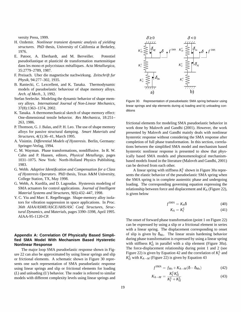
versity Press, 1999.H. Ozdemir. Nonlinear transient dynamic analysis of yielding

structures. PhD thesis, University of California at Berkeley,1976.

E. Patoor, A. Eberhardt, and M. Berveiller. Potentielpseudoelastique et plasticite de transformation martensitiquedans les mono et polycristaux metalliques. Acta Metallurgica,35:2779–2789, 1987.

F. Preisach. Uber die magnetische nachwirkung. Zeitschrift furPhysik, 94:277–302, 1935.

B. Raniecki, C. Lexcellent, and K. Tanaka. Thermodynamicmodels of pseudoelastic behaviour of shape memory alloys.Arch. of Mech., 3, 1992.

Stefan Seelecke. Modeling the dynamic behavior of shape mem-ory alloys. International Journal of Non-Linear Mechanics,37(8):1363–1374, 2002.

K. Tanaka. A thermomechanical sketch of shape memory effect:One-dimensional tensile behavior. Res Mechanica, 18:251–263, 1986.

P. Thomson, G. J. Balas, and P. H. Leo. The use of shape memoryalloys for passive structural damping. Smart Materials andStructures, 4(1):36–41, March 1995.

A. Visintin. Differential Models of Hysteresis. Berlin, Germany:Springer-Verlag, 1994.

C. M. Wayman. Phase transformations, nondiffusive. In R. W.Cahn and P. Haasen, editors, Physical Metallurgy, pages1031–1075. New York: North-Holland Physics Publishing,1983.

G. Webb. Adaptive Identification and Compensation for a Classof Hysteresis Operators. PhD thesis, Texas A&M University,College Station, TX, May 1998.

G. Webb, A. Kurdila, and D. Lagoudas. Hysteresis modeling ofSMA actuators for control applications. Journal of IntelligentMaterial Systems and Structures, 9(6):432–447, 1998.

Y. C. Yiu and Marc E. Regelbrugge. Shape-memory alloy isola-tors for vibration suppression in space applications. In Proc.36th AIAA/ASME/ASCE/AHS/ASC Conf. Structures, Struc-tural Dynamics, and Materials, pages 3390–3398, April 1995.AIAA-95-1120-CP.

Appendix A: Correlation Of Physically Based Simpli-fied SMA Model With Mechanism Based HystereticNonlinear Response

The major loop SMA pseudoelastic response shown in Fig-ure 22 can also be approximated by using linear springs and slipor frictional elements. A schematic shown in Figure 30 repre-sents one such representation of SMA pseudoelastic responseusing linear springs and slip or frictional elements for loading(L) and unloading (U) behavior. The reader is referred to similarmodels with different complexity levels using linear springs and

δ SMAf

Msδ

a)

0δ ≥�

Mfδδ SMAf

UIK

UIIIK

UIIK Afδ

b)

0δ <�

AsδLIIIK

LIK

LIIK

Figure 30. Representation of pseudoelastic SMA spring behavior using

linear springs and slip elements during a) loading and b) unloading con-

ditions

frictional elements for modeling SMA pseudoelastic behavior inwork done by Malovrh and Gandhi (2001). However, the workpresented by Malovrh and Gandhi mainly deals with nonlinearhysteretic response without considering the SMA response aftercompletion of full phase transformation. In this section, correla-tions between the simplified SMA model and mechanism basedhysteretic nonlinear response is presented to show that phys-ically based SMA models and phenomenological mechanism-based models found in the literature (Malovrh and Gandhi, 2001)can be derived from each other.

A linear spring with stiffness KLI shown in Figure 30a repre-

sents the elastic behavior of the pseudoelastic SMA spring whenthe SMA spring is in complete austenitic phase and undergoingloading. The corresponding governing equation expressing therelationship between force and displacement and KA (Figure 22),is given below

f SMA = KAδ (40)

KA = KLI (41)

The onset of forward phase transformation (point 1 on Figure 22)can be expressed by using a slip or a frictional element in serieswith a linear spring. The displacement corresponding to onsetof slip is given by δMs. The linear strain hardening behaviorduring phase transformation is expressed by using a linear springwith stiffness KL

II in parallel with a slip element (Figure 30a).The force-displacement relationship during point 1 and 2 (seeFigure 22) is given by Equation 42 and the correlation of KL

I andKL

II with KA→M (Figure 22) is given by Equation 43

f SMA = fMs +KA→M(δ−δMs) (42)

KA→M =KL

I KLII

KLI +KL

II(43)

19

The end of forward phase transformation and the strain harden-ing behavior seen afterwards (point 2 on Figure 22) can be repre-sented by using a linear spring with stiffness KL

III in parallel witha slip element with slip displacement δM f , acting against the dis-placement direction as shown in Figure 30. Corresponding force-displacement relationship and correlation of KL

I ,KLII and KL

III withKM is given by Equation 44 and Equation 45.

f SMA = fM f +KM(δ−δM f ) (44)

KM =KL

I KLIIK

LIII

KLIIK

LIII +KL

I KLIII +KL

I KLII

(45)

Figure 30b shows the schematic for unloading conditions.The slip element with corresponding slip displacement limit ofδM f during loading can be re-calibrated to a slip displacementof δAs for unloading conditions. This corresponds to point 3 onFigure 22 and represents start of phase transformation back intothe austenitic phase. The force-displacement relationship priorto reverse phase transformation is given by Equation 46, whereas, the relationship between KU

I ,KUII and KU

III with KM is givenby Equation 47.

f SMA = fAs +KM(δ−δAs) (46)

KM =KU

I KUII KU

III

KUII KU

III +KUI KU

III +KUI KU

II

(47)

The slip element with slip displacement of δMs during loadingcan be re-calibrated to a slip displacement of δA f for unload-ing conditions. This corresponds to point 4 on Figure 22 andrepresents end of phase transformation back into the austeniticphase. The force-displacement relationship during the reversephase transformation is given by Equation 48, where as the re-lationship between KU

I and KUII with KM→A is given by Equa-

tion 49.

f SMA = fA f +KM→A(δ−δA f ) (48)

KM→A =KU

I KUII

KUI +KU

II

(49)

After the end of reverse phase transformation the force varies lin-early with displacement proportional to KU

1 and the relationshipis same as shown in Equations 40 and 41.

Equations 40 to 43 represent SMA major loop responsebased on hysteretic nonlinear behavior using a combination oflinear springs with slip elements. Following a similar approach,expressions representing minor loop response can also be de-rived. However, since the purpose was only to show a correlationwith mechanism based models this task has not been performed.

20