كليـــــــــــــــــــــــــــــــــــة الهندســـــــــــــــــــــــــــــــــــــة

COLLEGE OF ENGINEERING

DEPARTMENT OF ELECTRICAL AND COMPUTER ENGINEERING

FINAL YEAR PROJECT PART II

ECCE 5099

Designing a Model for Losses Reduction in Loaded

Distribution Transformer

Done by:

Abdullah Suleiman Al-Wahaibi 52152/04

Haithem Yousuf Al- Ajmi 54548/04

Mundhir Yousuf Al- Bulushi 56467/04

Supervised by:

Dr. Abdullah Al- Badi

Dr. Asaad Al- Mudi

Prof. Dr. Ibrahim A. Metwally

ACADMIC YEAR

2008/2009

ABSTRACT

Losses in distribution transformers account for almost one third of overall transmission

and distribution losses. The efficiency of a typical modern power transformer is in

excess of 97%, which sounds perfectly satisfactory. However, this figure means that

up to 3% of all electrical power generated is wasted in transformer losses. These losses

are far from negligible, and anything that can be done to reduce them has the potential

to deliver huge savings, not just in monetary terms, but also in terms of reduced

environmental impact.

Energy is lost in a transformer, primarily in the form of wasted heat from changing

electrical and magnetic fields in the copper (windings), core, tank, and supporting

structure. Research over the last 50 years has succeeded in reducing no-load losses by

a factor of three while increasing core costs by a factor of two. Recent substitution in

distribution transformers (ratings below about 100 kVA) of amorphous metals for

silicon iron core material has reduced no-load losses further, but this material has not

been used in the cores of power transformers (ratings greater than 500 kVA) . In spite

of the fact that today's utility power transformer losses is less than 1% of its total

rating in wasted energy, any energy saved within this one percent represents a

tremendous potential savings over the expected lifetime of the transformer.

This project, talks about the transformer losses and its efficiency. Also, a model of a

transformer using MATLAB/SIMULINK and MATLAB/SIMPOWER is developed

and presented to calculate the losses in two conditions that the transformer can work

in, namely linear and saturable conditions. Finally, calculations for the total owning

cost are presented and discussed. This method provides an effective way to evaluate

various transformer initial purchase prices and cost of losses.

i

ii

الخالصة

انحالث انكشببئت كفبءة. حصعال قمالإجبن خغبئش ي رهذ السة ايب قحشكم ـ يحالث انخصع يفبقذال

3ش أ زا انشقى ع أ يب صم إن غ. بذسب حك يشضب حبيب ٪ 97حخجبص -رجت ال -انحذزت

ز انخغبئش ال ك انخؽبض عب ، كم . ـ خغبئش انحل٪ ي يجع انطبقت انكشببئت اننذة ضع ـ

.ةأضب ي انبئ، نظ ـقط ي انبحت انقذت ، بم عـش يببنػ ضخت يب ك انقبو ب نهحذ يب

طغت انكشببئت ـ انحبط اانجبالث انؽ ي حؽش ـقذ انحشاسةـ شكمحجنحل انطبقت انفقدة ـ ا

عبيب انبضت جح ـ انحذ ي خغعه يذ الانز ايخذ انبحذ. دعى انكم انخضا انصفبئح ( انهفبث)

اعخبذال حى ت األخشة ـ ا. أضعبـبيع صبدة انخكبنؿ األعبعت نك حجى انخغبئش أ بغبت رالرت أضعبؾ

عهك انحذذ انعبد نم انخؽشة انشكم( أيبش ـنجكه 100أقم ي ح انخ حقذسة)يحالث انخصع

يحالث ال صفبئحـ حغخخذوانخغبئش ، نك ز اناد نى ي انكزش خفضجبذسب انخ األعبعت انبدت

يحالث كشببئتعه انشؼى ي أ ـبئذة انو (أيبش ـنجكه 500أكبش ي ة انخ حصؿ ) ئتانكشبب

اناحذ أ طبقت يـشة داخم زا نك ي يجع انخصؿ ـ حبذذ انطبقت ، اناحذ ببنبئتخغبئش أقم ي ة

.عه يذ انعش انخقع نهحل حـشزم إيكببث بئهت ببنبئت

يم حصى ببعخخذاو عحى حذ .ـ انحالث انكشببئت كفبئخب انفبقذ زا انششع خحذد بقش

MATLAB/SIMULINK MATLAB/SIMPOWER نهحل انكشببئ نقبط ضبط انخغبئش انخ

انحالث انكشببئت ايخالك حكبنؿ يجع أخشا حى حغبة يبقشت . انخطت حبنت انخشبع: حخج ـ ـ حبنخ

.خفضبكفت

iii

ACKNOWLEDGMENT

First of all, we thank Allah who gives us the ability to do this project. Second, we

thank our advisors Dr. Abdullah Al-Badi, Dr. Asaad Al-Moudi and Prof. Dr. Ibrahim

Metwally for their help, sustaining and advice during the work time in this project.

Also, we are appreciating the help of Mazoon Electricity Company (MZEC), Dr.

Mohammed Majdi, Prof. Hassan Yosuf and Mr. Salem Al-Hinai and everybody who

contributes in this project even with little information.

iv

TABLE OF CONTENTS

ABSTRACT _________________________________________________________ i

ABSTRACT (Arabic) _________________________________________________ ii

AKNOWLEDGEMENT _______________________________________________ iii

TABLE OF CONTENTS ______________________________________________ iv

LIST OF TABLES ___________________________________________________ vii

LIST OF FIGURES _________________________________________________ viii

Chapter 1: Introduction

1.1: Background ____________________________________________________ 1

1.2: Project objectives _______________________________________________ 1

1.3: Report outline & organization _____________________________________ 2

Chapter 2: Literature Survey

2.1: Classification of the Transformer ___________________________________ 3

2.2: Main parts of transformer _________________________________________ 4

2.2.1: Transformer core ______________________________________________4

2.2.2: Windings ____________________________________________________5

2.2.3: Tanks ______________________________________________________ 6

2.2.4: Bushing _____________________________________________________7

2.3: Transformer Failures ______________________________________________8

2.4: On line Diagnostic Monitoring for Large Power Transformers ____________10

2.5: Parallel Operation of Transformers__________________________________11

2.6: Grounding System_______________________________________________19

2.6.1: Ungrounded System___________________________________________20

2.6.2: Solidly Grounded_____________________________________________22

2.6.3: Resistance Grounded__________________________________________23

v

2.6.4: Reactance Earthing____________________________________________24

2.7: Harmonics_____________________________________________________ 25

2.7.1: Impact of Harmonics on Transformer_____________________________26

2.7.2: Ways to measure the Waveform Distortion_________________________27

2.7.3: K-rated Transformer___________________________________________27

2.7.4: De-Rating Distribution Transformer ______________________________28

2.7.5: Filters______________________________________________________28

2.7.6: Power Factor________________________________________________30

2.7.7: Zig-Zag Transformer__________________________________________31

2.8: Summary______________________________________________________ 34

Chapter 3: Transformer Modeling and Simulation

3.1: Introduction ____________________________________________________35

3.1.1: Transformer Parameters _______________________________________ 35

3.2: Designing a Transformer model ____________________________________ 36

3.2.1: Linear Transformer model with balanced load ______________________36

3.2.1.1: No-Load condition for Linear Transformer (NLL) _______________ 37

3.2.1.2: Full-Load condition with balanced loads for Linear Transformer

(FLL) __________________________________________________ 37

3.2.2: Modeling a Saturable Transformer ______________________________ 39

3.2.2.1: Saturation with Balanced Loads ______________________________ 41

3.2.2.2: Saturation with Un-Balanced Linear Load ______________________45

vi

3.2.2.3: Saturation with Non-Linear Load ____________________________ 46

3.3: Conclusions ___________________________________________________ 51

Chapter 4: Transformer Efficiency

4.1: Introduction ___________________________________________________ 52

4.2: Matlab Simulation for 200 kVA and 500 kVA Distribution Transformer ____54

4.3: All Day Efficiency ______________________________________________ 55

4.3.1: Case Study _________________________________________________ 55

4.3.1.1: MATLAB Result _________________________________________ 56

4.4: Conclusions ____________________________________________________56

Chapter 5: Total Owning Cost

5.1: Introduction ___________________________________________________ 57

5.2: Design for minimum TOC ________________________________________57

5.3: Specifying A & B values _________________________________________ 59

5.3.1: Probabilistic Approach ________________________________________ 60

5.4: Discussion of Results ____________________________________________ 64

5.5: Conclusions ____________________________________________________66

Chapter 6: Conclusions and Future Work

6.1: Summary _____________________________________________________ 67

Appendices _________________________________________________________ I

References ______________________________________________________ XXII

vii

LIST OF TABLES

Table 2.1: Main monitoring on high-power transformers __________________11

Table 2.2: Harmonic Order vs. Phase Sequences_________________________26

Table 3.1: Transformer Equivalent circuit parameters for 200 kVA and 500

kVA___________________________________________________ 36

Table 3.2: Input and output powers and losses for FLL ____________________39

Table 3.3: Magnetizing Force and Current, Induction B and Flux Ф for 200 and

500 kVA________________________________________________40

Table 3.4: Input and output powers, the losses for BHL____________________43

Table 3.5: Input and output powers, the losses for BFL____________________44

Table 3.6: Input and output powers, the losses for un-balanced linear load ____ 45

Table 3.7: The percentage of harmonic components with respect to peak rated

current (377.13 A) ________________________________________48

Table 4.1: Maximum efficiency vs. power factor of 200 kVA and 500 kVA

distribution transformer ____________________________________55

Table 4.2: 24-hour energy cost_______________________________________ 55

viii

LIST OF FIGURES

Fig. 2.1: Transformer Classification __________________________________ 3

Fig. 2.2: Transformer Main Parts ____________________________________ 4

Fig. 2.3(a): Laminated shell Type ______________________________________ 4

Fig. 2.3(b): Laminated core Type _____________________________________ 4

Fig. 2.4: Transformer Cross-Sectional view with Windings _______________ 5

Fig. 2.5: Power Transformer 30 MVA 132/11 kV _______________________ 6

Fig. 2.6: Conservator Tank of Power Transformer ______________________ 6

Fig. 2.7: Transformer bushing type GOH _____________________________ 7

Fig. 2.8: Causes of Failures ________________________________________ 8

Fig. 2.9 Parallel operation of two single-phase transformer_______________13

Fig. 2.10: (a) Correct connection, (b) Wrong Connection__________________ 14

Fig. 2.11: Equivalent circuit for transformer working in parallel simplified circuit

and further simplification for identical voltage ratio______________ 16

Fig. 2.12: Equivalent circuit for unequal voltage ratio____________________ 17

Fig. 2.13: Grounding Methods_____________________________________ 20

Fig. 2.14: A Virtual Ground in Ungrounded System______________________ 21

Fig. 2.15: Solidly Grounded System_________________________________ 22

Fig. 2.16: Resistance Grounded System______________________________ 23

Fig. 2.17: Reactance Grounded System______________________________ 25

Fig. 2.18: Common Passive Filters Configuration_______________________ 29

Fig. 2.19: A Series Passive Filter___________________________________ 30

ix

Fig. 2.20: Transformer Zig-Zag of Connection Circuit____________________ 32

Fig. 2.21: Phasor Diagram of the Zig-Zag Transformer__________________ 32

Fig. 3.1: The equivalent circuit of the transformer______________________ 35

Fig. 3.2: Three-phase linear transformer ______________________________37

Fig. 3.3: Voltages and Currents for NLL _____________________________ 38

Fig. 3.4: Voltages and Currents for FLL _____________________________ 38

Fig. 3.5: Three Phase Saturable Transformer__________________________ 39

Fig. 3.6: Flux-current characteristic for 200 kVA and 500 kVA saturable

transformer_____________________________________________ 41

Fig. 3.7: Voltages and currents for BNL _____________________________ 42

Fig. 3.8: Voltages and currents for BHL _____________________________ 43

Fig. 3.9: Voltages and currents for BFL _____________________________ 44

Fig. 3.10: Voltages and currents for Un-balanced linear loads_____________ 45

Fig. 3.11: Full-Bridge rectifier load__________________________________ 46

Fig. 3.12: Primary and secondary voltages and currents for Full-Bridge rectifier

load __________________________________________________ 47

Fig. 3.13: Current harmonic spectrum________________________________ 47

Fig. 3.14: 5th

and 7th

filters inserted to a Full-Bridge Rectifier Load_________ 49

Fig. 3.15: Voltages and currents of the filtered Full-Bridge Rectifier________ 51

Fig. 4.1: Transformer losses ______________________________________ 52

Fig. 4.2: Power Loss vs. Percent load _______________________________ 54

Fig. 4.3: Power efficiency curves for 200kVA and 500kVA distribution

transformer at different load power factors ___________________ 54

x

Fig. 4.4: Loads and Efficiency Profile for 200 kVA ____________________ 56

Fig. 5.1: Transformer LCC Spreadsheet Model Flowchart _______________ 59

Fig. 5.2: The relation between A and n along life time___________________ 61

Fig. 5.3: The loading current annually for three years____________________ 61

Fig. 5.4: The relation between A and B_______________________________ 63

Fig. 5.5: The owning cost vs. the interest rate__________________________ 65

Fig. E: Open-Circuit Test _______________________________________ XII

Fig. F: Short-Circuit Test ______________________________________ XIII

1

Chapter 1: Introduction

1.1: Background

Electric power systems use transformers to change different voltage levels from higher

to lower or vice versa in order to transmit more power with high efficiency to utilities.

Each stage of the system can be operated at an appropriate voltage. In a typical system,

the generators in the power station deliver a voltage which is not suitable for

transmission purpose, then transformers step this voltage up for the long-distance

transmission. Higher voltages can be transmitted more efficiently over long distances

and have less losses. At the substation, the voltage may be transformed down to

distribution system at 11 kV or 33 kV. Finally the voltage is transformed once again at

the distribution transformer near the point of use to 240 V or 120 V.

1.2: Project Objectives

The objectives of this project are:

Designing a model for a losses reduction of a three phase loaded

distribution transformer.

Investigate the effect of loading one phase only on the transformer

efficiency and the losses in the power system.

Investigate the effect of the transformer size on the losses.

Calculate the cost of different distribution transformers.

2

1.3: Report outline & organization

This chapter is organized as the following:

Chapter one: is an introduction about the transformers.

Chapter two: Literature survey on different types of transformers and the

losses. Chapter three: Designing a model for a losses reduction of a three phase

loaded distribution transformer.

Chapter four: discusses the transformer efficiency and its classifications.

Chapter five: introduce the total owning cost of a transformer, and how the

total owning cost can be calculated, and the benefits of using this method.

Chapter six: concludes the study of the work completed. Future works are

presented in this chapter.

Finally, the report includes Appendices.

3

Chapter 2: Literature Survey

A power transformer is a device that has two or more coils wound on an iron core.

Transformers provide an efficient means of changing voltage and current levels, and

make the bulk power transmission system practical. The transformer primary is the

winding that accepts power, and the transformer secondary is the winding that delivers

power. The primary to secondary voltages is related by the turn's ratio of the coils. The

corresponding currents are related inversely by the same ratio. The transformers

operate on the principle of the electromagnetic induction [1].

Three-phase power transformer can be connected in four different ways depend on the

application. It can be connected as Y-∆, ∆-Y, Y-Y and ∆-∆. Y-∆ and ∆-Y produce

phase shift at the primary side by leading 30 or lagging 30, respectively [2].

2.1: Classification of the transformer

The power transformer is generally classified according to their size, insulation,

cooling method and location. Fig. 2.1 summarizes the transformer classification [3]:

Fig. 2.1: Transformer Classification.

Size

Power

Distribution

Insulation

Liquid immersed

Dry type

Gas Insulated

Super Conducting

Cooling Method

Self-Cooled

Forced Cooled

Location

Substation

Indoor

Pole-type

TRANSFORMER

4

2.2: Main parts of transformer

The main parts of the power and distribution transformers are: transformer core,

windings, tank and bushing [4].

Fig. 2.2: Transformer Main Parts [4].

2.2.1: Transformer core

Power transformers are constructed on one of two types of core. The first type is

known as shell type or shell form. This type consists of a three-legged laminated core

with the windings wrapped around the center lag as shown in Fig. 2.3 (a) [5]. The

second type is called the core type or core form. It consists of a simple rectangular

laminated piece of steel with the transformer windings wrapped around two sides of

the rectangle as can be shown in Fig. 2.3 (b). The core is constructed of thin

laminations electrically isolated from each other in order to reduce eddy currents to a

minimum [5].

Fig. 2.3: Types of laminated iron cores: (a) shell type and (b) core type [6].

(a) (a) (a)

(b)

5

The trend of using grain oriented silicon steel core for small distribution

transformer has charged since the introduction of the amorphous steel. Amorphous

steel core result in lower eddy current losses, narrow hysteresis loop also help to

reduce hysteresis. However the cost is higher by 25-30% compared to silicon steel.

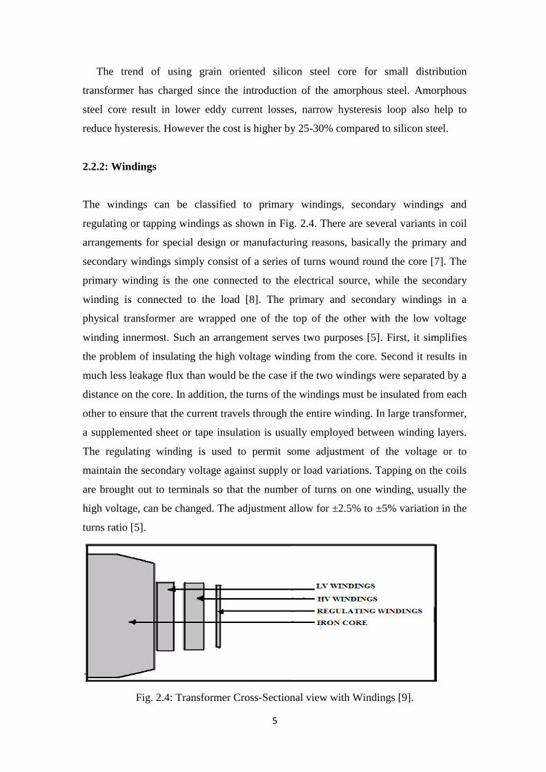
2.2.2: Windings

The windings can be classified to primary windings, secondary windings and

regulating or tapping windings as shown in Fig. 2.4. There are several variants in coil

arrangements for special design or manufacturing reasons, basically the primary and

secondary windings simply consist of a series of turns wound round the core [7]. The

primary winding is the one connected to the electrical source, while the secondary

winding is connected to the load [8]. The primary and secondary windings in a

physical transformer are wrapped one of the top of the other with the low voltage

winding innermost. Such an arrangement serves two purposes [5]. First, it simplifies

the problem of insulating the high voltage winding from the core. Second it results in

much less leakage flux than would be the case if the two windings were separated by a

distance on the core. In addition, the turns of the windings must be insulated from each

other to ensure that the current travels through the entire winding. In large transformer,

a supplemented sheet or tape insulation is usually employed between winding layers.

The regulating winding is used to permit some adjustment of the voltage or to

maintain the secondary voltage against supply or load variations. Tapping on the coils

are brought out to terminals so that the number of turns on one winding, usually the

high voltage, can be changed. The adjustment allow for ±2.5% to ±5% variation in the

turns ratio [5].

Fig. 2.4: Transformer Cross-Sectional view with Windings [9].

6

2.2.3: Tanks

The tank has two main parts [6]:

1- The tank is manufactured by forming and welding steel plate to be used as a

container for holding the core and coil assembly together with insulating oil. The tank

is designed to withstand the application of the internal overpressure specified without

permanent deformation.

2- The tank is equipped with an expansion reservoir (conservator) which allows for the

expansion of the oil during operation. The conservator is designed to hold a total

vacuum and may be equipped with a rubber membrane preventing direct contact

between the oil and the air.

Fig. 2.5 and Fig. 2.6 are illustrated the main parts of the tank.

Fig. 2.5: Power Transformer 30 MVA 132/11 kV [6].

Fig. 2.6: Conservator Tank of Power Transformer [6].

7

2.2.4: Bushing

The bushing is built up around a solid aluminum bolt which serves as a conductor for

both the current and for the heat losses as can be observed from Fig. 2.7. Cooling

flanges are milled directly in the conductor. The upper insulator, lower insulator and

mounting flange are held between the end plates by spring pressures. Sealing is

accomplished by oil-resistant rubber gaskets. The radial seal at the bottom end consists

of an O-ring made in a special fluorocarbon rubber. This material is very resistant to

high-temperature transformer oil, and has good flexibility in the lower temperature

range. The annular space between the condenser body and the porcelain is filled with

transformer oil. A gas-filled expansion space is left at the top [9].

The oil level can be checked by means of a dipstick in the oil filling hole. Both

insulators are made in one piece of high quality electrical porcelain. The mounting

flange is manufactured of corrosion resistant aluminum alloy. The mounting flange is

protected by painting with two component primer and a grey-blue finishing coat of

paint. The bushings are delivered oil filled and ready for use. The bushing can be

vertically or horizontally mounted. If the bushing is horizontally mounted, special

measures have to be taken to ensure sufficient oil filling in the bushing and

communication with an expansion space [9].

Fig. 2.7: Transformer bushing type GOH [9].

8

2.3: Transformer Failures

There are number of failures which affect the expected life of the transformer.

Transformer failures can occur as a result of different causes. Fig. 2.8 summarizes the

main causes of transformer failure and their percentage [10].

Fig. 2.8: Causes of Failures

1) OVERLOAD: A situation that results in electrical equipment carrying more

than its rated current. Placing large electrical load would cause an overload. The

main effect of overloading a transformer is increased heat. It can cause many

problems for the transformer such as damaging the insulation, creating short

circuits between the turns and also affecting the age of the transformer oil [10].

2) MOISTURE: Moisture in the solid part of power transformer insulation (paper,

pressboard) is one of the most critical condition parameters. Water enters

transformers from the atmosphere (breathing, leaky seals) and during

installation and repair. Moisture entering in oil-paper insulations can cause

dangerous effects

a) Decreases the dielectric withstand strength.

b) Causes the emission of gas bubbles at high temperatures and

may lead to a sudden electrical breakdown.

Assessing the moisture content in insulation is thus a key factor to ensure

transformer reliability and longevity [10].

0

5

10

15

20

25

30

35

Failu

re, %

9

3) LOOSE CONNECTON: This occurs due to improper mating of different

metals or improper torque of bolted connections, the loose connection can

cause the following problem to the transformer:

a) Spark between the cable and equipment.

b) Heating of any insulation.

c) Can ignite any inflammable material [10].

4) MANTENANCE ISSUES: This includes improperly set controls, loss of

coolant, and accumulation of dirt, oil and corrosion [10].

5) LIGHTNING: the main effect of the lighting on the transformer is the lighting

surges [10]. The surge can be defined as a short-duration (microsecond to

millisecond) increase in power line voltage, also called a spike or an impulse.

6) INSULATION ISSUES: the insulations in the transformers can be damaged due

to various reasons like lighting surges and overloaded [10].

7) ELECTRICAL DISTURBANCE: the electrical disturbance can occur due to the

following common reasons:

a) Surges: A line swell, also called a voltage surge, is a temporary

rise in the voltage level lasting at least one half cycles. Voltage swells can be caused

by high-power electric motors, switching off, and the normal cycling of HVAC

systems [11].

b) Voltage sags: line sag, sometimes called a voltage dip, is a

temporary decrease in the voltage level lasting at least one half cycle. Sags are usually

caused by sudden nearby increases in the electrical load and can degrade equipment

performance for several seconds at a time [11].

c) Voltage Transients or Spikes (Impulses): Sudden massive

increases in voltage, such as those caused by lightning striking a power line or the

nearby ground, can cause a damaging voltage pulse to enter electronic equipment and

destroy sensitive solid state circuitry. Lasting only a few milliseconds, storm induced

voltage transient spikes is responsible for huge losses every year [12].

d) Blackouts: During a blackout, all power is lost, ranging from

milliseconds to hours, or even longer. To keep critical equipment running, a new

power source must be provided either from stored energy (Uninterruptible Power

Supplies) or from a mechanical generator [11].

10

e) Brownouts: During periods of high power demand, the power

utility may intentionally reduce line voltage by up to 15%. Brownouts can last up to

several days and create many forms of abnormal equipment behavior [12].

f) Harmonics: Non-linear loads such as personal computers, office

equipment, variable frequency drives and solid-state electronics use switch mode

power supplies to generate DC voltage, sometimes causing currents that are out of

phase with voltage. These harmonics distort voltage waveforms, and can cause

overheating, nuisance tripping, and the loosening of electrical connectors [11].

8) OTHERS: it can be due manufacture errors, fire or explosion in area near to the

transformer [10].

2.4: On Line Diagnostic Monitoring for Large Power Transformers

Efficient diagnostic monitoring capable of highlighting incipient faults and therefore

able to reduce the fault rate and downtime of the transformer within considered

physiological limits are generally of extreme interest for maintenance departments

[12].

Diagnostic monitoring can be divided into on-line, if performed with the transformer

in normal operation and off-line, if the transformer requires to be powered down. They

can be used to:

a) Detect faults at an early stage and enable corrective measures in order to

prevent degeneration into catastrophic phenomena.

b) Monitor the ageing process of the insulating systems.

The table below summarizes the main things that need to be monitored on

transformers.

11

Table 2.1: Main Monitoring on High-Power Transformers [12].

Type of check Frequency

Dielectric rigidity of the oil annual

Water content in the oil annual

Chemical characteristics of the oil annual

Presence of corrosive sulphur in the oil Two - yearly

Chromatographic analyses of gases dissolved in the oil annual

Analysis of gases collected in the Buchholz relay Six - monthly

Thermometric check of hot points continuous

Measurement of tank vibrations Three - yearly

Measurement of acoustic emissions Three - yearly

Check of the cooling system Six - monthly

Tank monitoring Six - monthly

Check of other accessories Six - monthly

The gas in the oil is very important in online monitoring. In case of overheated, partial

discharge or local breakdown inside the transformer several gases are produced and

dissolved in the oil such as H2, CH4 and C2H6. If the generated gas is exceeding certain

limit, gas bubbles will arise. These gas bubbles can cause local breakdown if they

come into regions of the insulation system with high electric field strength.

2.5: Parallel Operation of Transformers

Most of the power transmission, distribution lines and transformers operate in parallel

to supply electricity. While running in parallel, one of transformers is selected as

master and the remaining as followers. The followers always change their tap positions

12

as done by the master. Transformers connected in parallel must have their tapings

interlocks system that should be active only in parallel operation. The interlock

prevents different tap settings on the parallel transformers from giving rise to an

excessive reactive current [13].

By parallel operation it means that two or more transformers are connected to the same

supply bus bars on the primary side and to a common bus bar/load on the secondary

side.

The reasons that necessitate parallel operation are as follows [14]:

1) Non-availability of a single large transformer to meet the total load

requirement.

2) The power demand might have increased over a time necessitating

augmentation of the capacity. More transformers connected in parallel will

then be pressed into service.

3) To ensure improved reliability. Even if one of the transformers gets into a fault

or is taken out for maintenance/repair the load can continued to be serviced.

4) To reduce the spare capacity. If many smaller size transformers is used one

machine can be used as spare. If only one large machine is feeding the load, a

spare of similar rating has to be available. The problem of spares becomes

more acute with fewer machines in service at a location.

5) When transportation problems limit installation of large transformers at site, it

may be easier to transport smaller ones to site and work them in parallel.

Fig. 2.9 shows two single phase transformer connected in parallel, transformer A and

Transformer B are connected to input voltage bus bars. After ascertaining the

polarities they are connected to output/load bus bars.

13

Fig. 2.9: Parallel operation of two single-phase transformers.

The theoretically ideal conditions for paralleling transformers are:

1) The turns ratio and voltage ratio must be the same.

2) The per unit impedance of each transformer on its own base must be the same.

3) Equal ratios of resistance to reactance.

4) Same polarity, so there is no circulating current between the transformers.

5) The phase sequence must be the same and no phase difference must exist

between the voltages of the two transformers.

When two transformers are connected in parallel they must satisfy all the conditions in

order to avoid the circulating current.

Turns Ratio and Voltage Ratio

Generally the turns ratio and the voltage are taken to be the same, If the ratio is large

there can be considerable error in the voltages even if the turns ratios are the same.

When the primaries are connected to same bus bars, if the secondaries do not show the

same voltage, paralleling them would result in a circulating current between the

secondaries [15]. If the turns ratio are different the output voltages E2A and E2B will

not be equal and a current will circulate in the closed loop formed by the two

secondaries as it shown in Fig. 2.9.

14

The effect of per unit impedance

Transformers of different ratings may be required to operate in parallel. Thus the

larger machines have smaller impedance and smaller machines must have larger ohmic

impedance. Thus the impedances must be in the inverse ratios of the ratings. In

addition if active and reactive powers are required to be shared in proportion to the

ratings the impedance angles also must be the same. Thus we have the requirement

that per unit resistance and per unit reactance of both the transformers must be the

same for proper load sharing.

The effect of polarity

Correct polarity is important when transformers are connected in parallel to supply the

same load. Other ways, there will be circulating current. The polarity of connection

in the case of single phase transformers can be either same or opposite. If wrong

polarity is chosen the two voltages get added and short circuit results. Transformers

having −30◦ angle can be paralleled to that having +30

◦ angle by reversing the phase

sequence of both primary and secondary terminals of one of the transformers. This

way one can overcome the problem of the phase angle error. Fig. 2.10 shows the

wrong connection and correct connection.

Fig. 2.10 (a) correct connection, (b) wrong connection.

15

The effect of phase sequence

The poly phase banks belonging to same vector group can be connected in parallel. A

transformer with +30◦ phase angle however can be paralleled with the one with −30

◦

phase angle; the phase sequence is reversed for one of them both at primary and

secondary terminals. If the phase sequences are not the same then the two transformers

cannot be connected in parallel even if they belong to same vector group. The phase

sequence can be found out by the use of a phase sequence indicator.

Performance of two or more single phase transformers working in parallel can be

computed using their equivalent circuit. In the case of poly phase banks also the

approach is identical and the single phase equivalent circuit of the same can be used.

Basically two cases arise in these problems. Case A: when the voltage ratio of the two

transformers is the same and Case B: when the voltage ratios are not the same.

Case A: Equal Voltage Ratios

Always two transformers of equal voltage ratios are selected for working in parallel.

This way one can avoid a circulating current between the transformers. Load can be

switched on subsequently to these bus bars. Neglecting the parallel branch of the

equivalent circuit the above connection can be shown as in

Figs. 2.11 (a) and (b). The equivalent circuit is drawn in terms of the secondary

parameters. This may be further simplified as shown under Fig. 2.11(c). The voltage

drop across the two transformers must be the same by virtue of common connection at

input as well as output ends.

16

Fig. 2.11: Equivalent circuit for transformers working in parallel simplified circuit and

further simplification for identical voltage ratio.

From the figure we note:

VIZZIZI BBAA (2.1)

BA III (2.2)

Z is the equivalent impedance of the two transformers given by,

BA

BA

ZZ

ZZZ

(2.3)

BA

A

BB

B

BA

B

AA

A

ZZ

ZI

Z

IZ

Z

VI

ZZ

ZI

Z

IZ

Z

VI

.

.

(2.4)

17

If the terminal voltage is LZIV then the active and reactive power supplied by

each of the two transformers is given by

)(Re *

AA VIalP and )(Im *

AA VIagQ (2.5)

)(Re *

BB VIalP and )(Im *

BB VIagQ (2.6)

From the above it is seen that the transformer with higher impedance supplies lower

load current and vice versa. If transformers of dissimilar ratings are paralleled the

transformer with larger rating shall have smaller impedance as it has to produce the

same drop as the other transformer, at a larger current. Thus the ohmic values of the

impedances must be in the inverse ratio of the ratings of the transformers.

Case B: Unequal voltage ratio

Due to manufacturing differences, even in transformers built as per the same design,

the voltage ratios may not be the same. In such cases the circuit representation for

parallel operation will be different as shown in Fig. 2.12.

Fig. 2.12: Equivalent circuit for unequal voltage ratio.

18

It has been already mentioned that a small difference in voltage ratios can be tolerated

in the parallel operation of transformer, the two mesh voltage balance equations can be

written as:

AALLBAAAA ZIVZIIZIE )( (2.7)

BBLLBABBB ZIVZIIZIE )( (2.8)

Solving the two equations for AI and BI we can obtain:

)(

)(

BALBA

LBABAA

ZZZZZ

ZEEZEI

(2.9)

)(

)(

BALBA

LABABB

ZZZZZ

ZEEZEI

(2.10)

AZ and BZ are phasors and hence there can be angular difference also in addition to

the difference in magnitude.

At no load there will be a circulating current between the transformers. The currents

in that case can be obtained by putting LZ = 1 (after dividing the numerator and the

denominator by LZ ). Then the circulating current between two transformers is given

by,

BA

BABA

ZZ

EEII

(2.11)

On short circuit if the load impedance becomes zero:

B

BB

A

AA

Z

EI

Z

EI , (2.12)

On loading:

A

BBBAA

Z

ZIEEI

)( (2.13)

When two transformers are connected in parallel, the impedances of the transformers

must match (within 10%) to divide the load approximately equally between the two

transformers or to divide the load according to the rating of each transformer. If the

19

transformers to be connected in parallel are equipped with load tap changing windings,

then the impedances for each of the tap changer positions must match. If these

conditions are not met, then one of the transformers could conceivably carry a

continuous overload, resulting in overheating [15], when transformers are connected in

parallel, their impedances must match to ensure that neither transformer is subject to

an overload. This presents a problem with an LTC transformer, since its impedance

varies.

2.6: Grounding System

Grounding is used to stabilize the line to ground voltage during normal operations, and

it limits voltage during abnormal surges such as lightning or accidental contact with

higher voltage lines.

All of these goals help to improve safety and minimize damage. However, not all

power systems are solidly grounded. Depending on the NEC requirements for a given

system, there may be a choice between types of grounding so consideration must be

given to the advantages and disadvantages of each. Whether the choice is solidly

grounded, ungrounded or impedance grounded, the type of grounding used will affect

many variables. The single biggest impact is on the magnitude of current that could

flow due to a ground fault and the possible damage that the current could create [16].

Grounding has many objectives. It provides a common point of reference to the life

electrical conductors of a power supply network. It provides a path for surge currents

to flow to the soil mass. It ensures safety by clamping the exposed conducting

enclosure of electrical equipment at ground potential. Correct grounding practices go a

long way in controlling and mitigating electrical noise. Improper grounding can result

in many problems in the power system and associated control and communication

systems. Grounding is thus variously classified depending on the function performed

by it as: system grounding, protective grounding, lightning/surge protection grounding

or signal reference ground planes for noise mitigation in sensitive circuits. An engineer

dealing with power supply networks needs to understand the basic principles of

grounding system design and its role in ensuring safety of equipment and personnel. A

correct understanding of the basic principles involved will help him/her to avoid

20

mistakes in grounding system design, mistakes that could lead to expensive failures

and long downtime. Fig. 2.13 summarizes the method of grounding [17].

Fig. 2.13: Grounding Methods.

2.6.1: Ungrounded System

Providing a reference ground in any electrical system is crucial for safe operation,

although sometimes a system can be operated without it. An ungrounded system is an

electrical system that is not connected to the ground. However, a ground connection

does exist due to capacitances between the live conductors and ground. But this

capacitive reactance cannot provide a reliable reference because they are very high, as

seen in Fig. 2.18. Sometimes, the neutral of potential transformer primary windings

connected to the system is grounded, thus giving a ground reference to the system

[17].

System Grounding

Ungrounded Grounded

Impedance Grounding

Resistance

Low Resistance

High Resistance

Reactance

Low Reactance

High Reactance

Soild Grounding

21

Fig. 2.14: A Virtual Ground in an Ungrounded System.

S: Source of voltage.

ZL: Impedance of line conductor to ground

(Combination on insulation resistance and Line to ground capacitance).

Zg: Impedance of neutral conductor to ground.

Normally ZL = Zg therefore VL=Vg = V/2.

The advantages of the ungrounded system:

1) When there is a fault in the system involving ground the resulting currents

are so low that they do not cause an immediate problem to the system. The

system can resume without interruption which is important when an outage

will be expensive in terms of lost production or can give rise to life

threatening emergencies [17].

2) Reducing the overall cost of the system [17].

The Disadvantages of the Ungrounded System:

1) In all small electrical systems, the capacitances between the system

conductors and the ground can result in the flow of capacitive ground fault

current at the faulted point. This can cause repeated arcing and build up of

excessive voltage with reference to ground. This is far more destructive and

can cause multiple insulation failures in the system at the same instant [17].

2) Detecting the exact location of the fault takes far more time than with

grounded systems. This is because the detection of fault is usually done by

means of a broken Delta connection in the voltage transformer circuit. This

22

arrangement does not tell where a fault has occurred and to do so, a far

more complex system of ground fault protection is required which negates

the cost advantage [17].

3) A second ground fault occurring in a different phase when one unresolved

fault is present will result in a short circuit in the system [17].

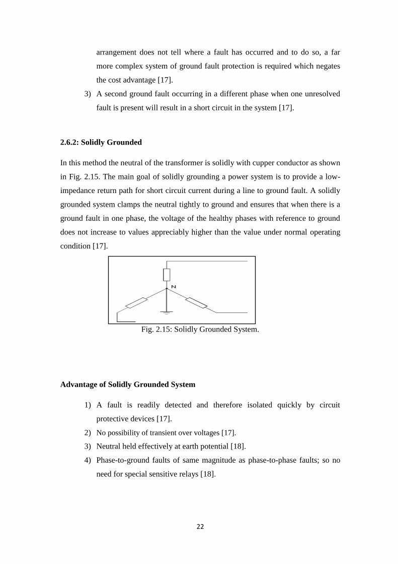
2.6.2: Solidly Grounded

In this method the neutral of the transformer is solidly with cupper conductor as shown

in Fig. 2.15. The main goal of solidly grounding a power system is to provide a low-

impedance return path for short circuit current during a line to ground fault. A solidly

grounded system clamps the neutral tightly to ground and ensures that when there is a

ground fault in one phase, the voltage of the healthy phases with reference to ground

does not increase to values appreciably higher than the value under normal operating

condition [17].

Fig. 2.15: Solidly Grounded System.

Advantage of Solidly Grounded System

1) A fault is readily detected and therefore isolated quickly by circuit

protective devices [17].

2) No possibility of transient over voltages [17].

3) Neutral held effectively at earth potential [18].

4) Phase-to-ground faults of same magnitude as phase-to-phase faults; so no

need for special sensitive relays [18].

23

5) Cost of current limiting device is eliminated because the protection against

short circuit faults (such as circuit breakers or fuses) is suitable to sense and

isolate ground faults as well [18].

6) Grading insulation towards neutral point N reduces size and cost of

transformers [18].

Disadvantage of Solidly Grounded System:

1) Distribution circuits of higher voltage (5 kV and above), the very low ground

impedance results in high ground fault currents almost equal or higher than the

system‟s three phase short circuit currents. This can increase the rupturing duty

ratings of the equipment to be selected in these systems. This fault have serious

effect when the fault occur inside the devices such as motors or generators, so

solidly grounded is usually applied for system lower than (380/480 V) [17].

2) Third harmonics tend to circulate between neutrals [18].

2.6.3: Resistance Grounded

A resistor is connected between the transformer neutral and earth as shown in Fig.

2.16. This method mainly used in systems below 33kV [18]. The value of the

resistance is selected such that to limit the earthed fault current to between 1 and 2

times full load rating of the transformer. Alternatively, to twice the normal rating of

the largest feeder, whichever is greater [18].

Fig. 2.16: Resistance Grounded System

24

Advantage of Resistance Grounding

1) Reducing damage to active magnetic components by reducing the fault

current [17].

2) Minimizing the fault energy so that arc flash effects are minimal thus

ensuring safety of personnel near the fault point [17].

3) Avoiding transient over voltages and the resulting secondary failures [17].

4) Reducing momentary voltage dips, which can be caused if, the fault

currents were higher as in the case of a solidly grounded system [17].

5) Obtaining sufficient fault current flow to permit easy detection and

isolation of faulted circuits [17].

High resistance grounding limits the current to about 10 A. But to ensure that transient

over voltages do not occur, this value should be more than the current through system

capacitance to ground. Low resistance grounding is designed for ground fault currents

of 100 A or more with values of even 1000 A being common. This method is most

commonly used in industrial systems and has all the advantages of transient limitation,

easy detection and limiting severe arc or flash damages from happening [17].

The resistance value is so chosen that:

The resulting ground fault current can be detected easily [17].

It does not become high enough to cause internal (core damage) when a

ground fault takes place in a rotating machine or a generator [17].

The resistive component of the current is not lower than 3 times the

capacitive component of ground fault current [17].

Disadvantage of Resistance Grounding

Full line-to-line insulation required between phase and earth [18].

2.6.4: Reactance Earthing

A reactor is connected between the transformer neutral and earth as shown in

Fig. 2.17 the value of the reactance is selected almost same as in resistance grounding.

To achieve the same value as the resistor, the design of the reactor is smaller and thus

cheaper [18]. This method limit ground fault current since it is a function of the phase

to neutral voltage and the neutral impedance. It is usual to choose the value of the

grounding reactor in such a way that the ground fault current is restricted to a value

25

between 25% and 60% of the three phase fault current (to prevent the possibility of

transient over voltages occurring).

Fig. 2.17: Reactance Grounded System

2.7: Harmonics

Nowadays, the number of non-linear loads, which draw non-sinusoidal currents even if

fed with sinusoidal voltage, connected to the power supply system are large and

continue to grow rapidly. These currents can be defined in terms of a fundamental

component and harmonic components of higher order [19].

In power transformers, the main consequence of harmonic currents is an increase in

losses, mainly in windings, because of the deformation of the leakage fields. Higher

losses mean that more heat is generated in the transformer so that the operating

temperature increases, leading to deterioration of the insulation and a potential

reduction in lifetime [19].

Modern transformers use alternative winding designs such as foil windings or mixed

wire/foil windings. For these transformers, the standardized K-factor – derived for the

load current - does not reflect the additional load losses and the actual increase in

losses proves to be very dependent on the construction method. It is therefore

necessary to minimize the additional losses at the design stage of the transformer for

the given load data using field simulation methods or measuring techniques [19].

Harmonics, by definition, occur at the steady state and are integer multiples of the

fundamental frequencies. The wave-form distortion that produce harmonics is present

continually; or at least for several seconds. Zero, positive and negative sequences can

be found from the equation (2.14), (2.15) and (2.16) respectively [20].Table 2.2 shows

harmonics orders vs. phase sequence [21].

26

n = 3 × m (2.14)

n = 3 × (m-2) (2.15)

n = 3 × (m-1) (2.16)

where: m = 1, 2, 3, 4, ……

Table 2.2: Harmonic Order vs. Phase Sequence

Harmonic Order Sequence

1, 4, 7, 10, 13, 16, 19 Positive

2, 5, 8, 11,14, 17,20 Negative

3, 6, 9, 12, 15, 18, 21 Zero

2.7.1: Impact of Harmonics on Transformer

Transformers are designed to deliver the required power to the connected load with

minimum losses at fundamental frequencies. Harmonics distortion of the current, in

particular, as will as of the voltage will significantly contribute to additional heating.

To design transformer to accommodate higher frequencies, designers make different

design choices such as continuously transposed cable instead of solid conductor and

putting in more cooling ducts. As general rule, a transformer in which the current

distortion exceeds 5% is a candidate for derating for harmonics [22].

When the load current includes harmonics there are two effects that result in increased

transformer heating:

1) RMS current. If the transformer is sized only for the kVA requirements of the

load, harmonics current may result in the transformer rms current being higher

than its capacity. The increased total rms current results in increased conductor

losses [22].

2) EDDY current losses. These are induced currents in a transformer caused by

the magnetic fluxes. These induced currents flow in the windings, in the core,

and in the other conducting bodies subjected to the magnetic field of the

transformer and cause additional heating. This component of the transformer

27

losses increases with the square of the frequency of the current causing the

eddy currents. Therefore, this becomes a very important component of the

transformer losses for harmonics heating [22].

2.7.2: Ways to Measure the Waveform Distortion

1) Total Harmonic Distortion (THDI): is the ratio of the RMS value of the total

harmonics currents (Non-fundamental part of the wave form) and the RMS of the

fundamental portion of the wave form. This value usually expressed as percentage of

the fundamental current [23].

1

22

2

1

N

h

h

I

I

THDI

(2.17)

where, Ih and I1 are the harmonic and the fundamental currents respectively.

Harmonic current distortion greater than 5% will contribute to the additional heating

of power transformers, so it must be derated for harmonics.

2) CREST FACTOR: is the ratio of peak wave form to its RMS value [22].

peak

rms

ICREST FACTOR

I (2.18)

2.7.3: K-Rated Transformer

This K-rated are marked on some transformers and it indicates the ability of the

transformer to supply loads which producing harmonics currents. A pure linear load –

one that draws a sinusoidal current – would have a K-factor of unity. A higher K-

factor indicates that the eddy current loss in the transformer will be K times the value

at the fundamental frequency. „K-rated‟ transformers are therefore designed to have

very low eddy current loss at fundamental frequency [19]. Standard transformer

ratings are K-4, K-9, K-13, K-20, K-30, K-40 and K-50 [23]. K-factor of K-4 or K-9

indicates the transformer can supply the rated current to loads that would increase the

eddy current losses of K-1 transformer by a factor of 4 or 9 respectively. Transformers

rated K-9 or K-13 would likely be required for office area containing many desktops

28

computers, copy machines, fax machines and electronic lighting ballasts. A large

variable-speed motor drive could required transformer rated K-30 or higher [24]. The

higher the K-rating, the greater is the ability of the transformer to supply loads that

have a higher percentage of harmonics current producing equipment without

overheating. The value of K can be determined by using Equation (2.19) [25] and a

case study is given in Appendix A.

2 2

1

n

pu

h

K I h

(2.19)

Nonrated K=1 transformers when the load produce harmonics currents less

than 15% of the total load [25].

K-4 rated transformers when the load produces harmonics currents are 15% to

35% of the total load [25].

K-13 rated transformers when the load produces harmonics currents are 35% to

75% of the total load [25].

K-20 rated transformers when the load produces harmonics currents are 75% to

100% of the total load [25].

K-30 and higher rated transformer for specific equipment where the load and

transformer are matched for harmonics characteristics [25].

2.7.4: De-Rating Distribution Transformers

Derating is a means of determining the maximum load that may be safely placed on a

transformer that supplies harmonic loads. The most common derating method is the

CBEMA approved "crest factor" method which provides a transformer harmonic

derating factor, THDF [24]. Appendix B shows the case study and its calculation.

1.414 True RMS of the Phase CurrentTHDF

Peak of the Phase Current

(2.20)

2.7.5: Filters

As mentioned at the beginning of this report non-linear load such as AC or DC

Adjustable Speed Drive (ASD), power rectifiers and inverters, arc furnaces, and

discharge lighting (metal halide, fluorescent…etc) and even saturated transformer.

These non-linear loads can cause harmonics which are enough to produce distorted

29

current and voltage wave's shapes. The main impact of the harmonics on the

equipment is overheating because of the presence of the harmonics in addition of the

fundamental. Harmonics can be mitigated using passive and active filters. Passive

filter are consists of tunable L-C circuit, are most popular. However, they required

careful application, and may produce unwanted side effects, particular in the presence

of power factor correction capacitors [24].

Passive filters are constructed from using passive elements (resistors, capacitors,

inductors). Theses filters are used in three phase, 4 wires distribution systems. They

are located close to the loads. Harmonics can be reduced to 30% by using passive

filters [25]. They are commonly used. However they have disadvantage of potentially

interacting adversely with the power system. It is important to check all possible

system interactions when they are designed. They are used either to shunt the

harmonics currents off the line or to block their flow between parts of the system by

tuning the elements to create a resonance at a selected frequency [22]. Fig. 2.18 shows

the common types of passive filters.

Fig. 2.18: Common Passive Filters Configuration.

Shunt Passive Filters: single tuned or “notch filter” is the most common type of

passive filters. Its series tuned to provide low impedance to particular harmonic

current. And it‟s connected in a shunt with the power system. Thus, the harmonic

currents are diverted from normal path on the line through filter. Notch filters can

provide power factor correction in addition to harmonic suppression. In fact, the power

factor correction capacitors may be used to make notch-filter[22].

30

Series Passive Filters: it‟s connected in series with the load. The inductance and the

capacitance are connected in parallel so that it provide high impedance at selected

harmonic frequency, so the high impedance then blocks the flow of harmonics current

at tuned frequency only. At the fundamental frequency, the filter is designed to

provide low impedance, thereby allowing the fundamental current to flow with only

minor additional impedance and losses. Fig. 2.19 shows a typical series filter [22].

Fig. 2.19: A series Passive Filter.

Series filters are used to block a single harmonic current (like 3rd

order only) so it‟s

useful in a single phase circuit, where it‟s not possible to take advantage of zero-

sequence characteristics. Series filters are designed to carry the full rated load current

and must have an over-current protection scheme [22].

2.7.6: Power Factor

Power factor is very important issue in electrical system because low power factor

may cause electrical equipments to fail and also the cost of low power factor can be

high; utilities penalize facilities that have low power factor because they find it

difficult to meet the resulting demands for electrical energy. In power system if the

power factor is 0.8 means that only 80% of the apparent power will convert into useful

work. Apparent power is what the transformer that serves a home or business has to

carry in order for that home or business to function. Active power is the portion of the

apparent power that performs useful work and supplies losses in the electrical

equipment that are associated with doing the work. Higher power factor leads to more

optimum use of electrical current in a facility. Power factor cannot reach 1 because all

electrical circuits have inductance and capacitance, which introduce reactive power

requirements. The reactive power is that portion of the apparent power that prevents it

from obtaining a power factor of 100% and is the power that an AC electrical system

requires in order to perform useful work in the system. Reactive power sets up a

magnetic field in the motor so that a torque is produced. It is also the power that sets

31

up a magnetic field in a transformer core allowing transfer of power from the primary

to the secondary windings. There are two terminology used in power factor studies,

displacement and true power factor. Displacement power factor is the cosine of the

angle between the fundamental voltage and current waveforms. But, if the waveform

distortion is due to harmonics, the power factor angles are different than what would

be for the fundamental waves alone. The presence of harmonics introduces additional

phase shift between the voltage and the current. True power factor is calculated as the

ratio between the total active powers used in a circuit (including harmonics) and the

total apparent power (including harmonics) supplied from the source. Two ways to

improve the power factor and minimize the apparent power drawn from the power

source are [26]:

1) Reduce the lagging reactive current demand of the loads.

2) Compensate for the lagging reactive current by supplying leading reactive

current to the power system.

There several advantage for correcting power factor:

1) Reduced heating in equipment.

2) Increased equipment life.

3) Reduction in energy losses and operating costs.

4) Freeing up available energy.

5) Reduction of voltage drops in the electrical system.

2.7.7: Zig-Zag Transformer

The Zig-Zag connection is also called the “interconnected star connection”. It‟s used

in commercial facilities to control zero-sequence current by providing a low

impedance path to neutral. This reduces the amount of current that flows in the neutral

back toward the supply by providing a shorter path for the current. In practical the

transformers located near the load [27].

Zig-Zag transformer is a special connection of three single-phase transformer‟s

windings or a three-phase transformer‟s windings. The circuit connection is as shown

in Fig. 2.20 below [27].

32

Fig. 2.20: Transformer Zig-Zag of Connection Circuit.

The three-phase zero-sequence currents (ia0, ib0, ic0) have the same amplitude and the

same phase, and the neutral current equal to the sum of the three components. Because

the turn ratio of the transformer‟s windings is 1:1 in Fig. 2.20, the input current

flowing into the dot point of the primary winding is equal to the output current flowing

out from the dot point of the secondary winding. Then, we can obtain iza=izb ,izb= izc

and izc= iza. This indicates that the three-phase currents flowing into three transformers

must be equal. This means that the Zig-Zag transformer can supply the path for the

zero-sequence current. Figure 2.21 shows the phasor diagram of Fig. 2.20 From Fig.

2.21, it can be found that the voltage across the transformer‟s winding is (1/1.7321) of

the phase voltage of the three-phase four-wire distribution power system [27].

Fig. 2.21: Phasor Diagram of the Zig-Zag Transformer.

Feeders Rearrangement

Feeder Rearrangement is another method to minimize loss. This is controlled by

switches. In any power system, there are two types of switches. Sectionalizing

33

switches are usually closed and are used to connect line sections. Tie-switches, on the

other hand, are normally open and are used to connect two primary feeders or two

substations, or loop type laterals. To observe how these switches control the feeders, it

is essential first to understand the mechanism of distribution lines [28].

Each distribution line has distinct characteristics, because each one has different

mixture of residential, commercial and industrial type of loads. Corresponding peak

time of distribution lines is not coincident, because distribution systems are loaded

differently at different times. At one time they would be heavily loaded, while at other

times, the load will be minor. Therefore, it is essential to alter the radial structure of

the distributing feeders. This is done by shifting the loads in the system, which not

only reduce transformer overload, but also minimizes real power loss [28].

Feeder‟s reconfiguration is done by changing the status of the above mentioned

switches. Most electrical distribution networks are operated radially, and therefore, the

change in the switches status in this way preserves radiality. When line losses are

minimized without any violating branches-loading and voltage limits, optimal

operation condition of distribution networks is obtained [28].

Feeder reconfiguration is done in several methods. Examples of early methods are:

linear programming method, branch and bound method, and the quasi-quadratic

nonlinear programming technique. Nevertheless, these methods were inefficient in

real-time application due to time consumption and the large number of iterations

required solving the load flow of the system. The most efficient of reconfiguration of

feeders is “the minimal tree-search” which finds many possible switching-options for

loss reduction [28].

34

2.8: Summary

Transformers are classified according to their size, insulation, cooling method

and location. The main parts of the transformer are windings, core, insulators,

tank and the bushing.

Cores are usually made of silicon steel but recently the manufacturers use

amorphous iron because of its lower eddy current losses and narrow hysteresis

loop.

There are number of failures which affect the transformer life time.

Transformer failures can occur as a result of different causes. The most

common failures are electrical disturbances, insulation issues and lightning.

Most of the power transmission, distribution lines and transformers operate in

parallel to supply electricity. While running in parallel, one of transformers is

selected as master and the reaming as followers.

The theoretically ideal conditions for paralleling transformers are: The turns

ratio and voltage ratio must be the same, the per unit impedance of each

machine on its own base must be the same, Equal ratios of resistance to

reactance, Same polarity and the phase sequence must be the same. When two

transformers are connected in parallel they must satisfy all the conditions in

order to avoid the circulating current.

Harmonics currents results from non-linear loads. The main impact of

harmonics is increasing in loses, mainly in windings, because of the

deformation of the leakage field.

The higher the K-rating the greater is the ability of the transformer to supply

loads that have a higher percentage of harmonics current producing equipment

without overheating. This methods used in countries that follow American

standard. Appendix A show how the K factor is calculated.

Passive filters are commonly used in reducing harmonics currents, by

providing low impedance path to particular harmonic current and they are

located closed to the load.

The neutral point of the transformer is grounded solidly or via impedance.

Impedance means low or high resistance or low or high reactance. Each

method has advantages and disadvantages. By using National Electrical Code

(NEC) the methods of grounding can be determined.

35

Chapter 3: Transformer Modeling and Simulation

3.1: Introduction

Losses are the main issue that faces any device in real life, so it is very important to

detect, quantify and reduce the losses as much as possible. To identify the losses inside

the transformers, MATLAB/SIMULINK/SIMPOWER is used. SIMULINK is a

program with graphical programming facilities for simulating dynamic systems while

SIMPOWER Systems extends SIMULINK with tools for modeling and simulating the

generation, transmission, distribution, and consumption of electrical power [29]. A

model is developed to identify the losses in 200 kVA and 500 kVA distribution

transformer.

3.1.1: Transformer Parameters

In order to model a transformer, there are some parameters that should be calculated

and provided. From the data-sheets provided from Mazoon Electricity Company

(MZECO) that are shown in Appendixes C.1 and C.2, the parameters of the

transformer were calculated from the equivalent circuit by using a MATLAB model

(Appendix D). Table 3.1 presents the parameters for the 200 kVA and 500 kVA

distribution transformer. The parameters were obtained from the equivalent circuit of

the open circuit and short circuit tests. These two tests are shown and discussed in

Appendices E and F respectively. The transformer used in the model is a distribution

transformer 200 kVA, 11 kV/ 433V (∆-Y connection), 50 Hz and also assuming the

load power factor to be 0.9 lagging. The model takes into account 1R , 2R , the leakage

inductance 1L and 2L as well as the magnetizing characteristic of the core, which is

modeled by a resistance cR simulating the core losses and mL . The corresponding

equivalent circuit for the transformer is shown in Fig. 3.1.

Fig. 3.1: Transformer Equivalent Circuit.

Fig. 3.1: The equivalent circuit of the transformer.

36

Table 3.1: Transformer Equivalent circuit parameters for 200 kVA and 500 kVA

Parameters 200 kVA 500 kVA

1R 14.75 3.222

1X 41 16.94

1L 0.131 H 0.054 H

2R 0.0062 0.0017

2X 0.021 0.00875

2L 0.067 mH 0.028 mH

eqR 26.75 6.54

eqX 82 33.86 k

eqZ 86.2 34.5

cR 728 k 366.67 k

mX 101 k 26.3 k

mL 321.5 H 83.72 H

3.2: Designing a Transformer model

3.2.1: Linear Transformer model with balanced load

In this section a model for a three-phase linear transformer will be designed and

analyzed at two conditions; full-load and no-load. For each of these two conditions,

the total power will be calculated; the waveforms for the currents, voltages,

magnetizing currents and fluxes will be obtained. The MATLAB/SIMULINK model

for the linear transformer is shown in Fig. 3.2. All the voltages and currents presented

are in Volts (V) and Amps (A), respectively.

37

Fig. 3.2: Three-phase linear transformer.

3.2.1.1: No-Load condition for Linear Transformer (NLL)

In this case, the load from the secondary-side is removed (open circuit) as can be

observed in Fig. 3.3 that the secondary current is equal to zero. The rms voltages and

the currents that flow in the primary and the secondary are shown in Appendix G.

3.2.1.2: Full-Load condition with balanced loads for Linear Transformer (FLL)

In the Full-Load condition, the load -which is defined as an RL-load - will consume

the whole power that is given (200 kVA). In this case, the RL-load is adjusted to have:

60 kW real powers and 29.1 kVAr per phase in order to consume the whole power.

Fig. 3.3 shows the voltages and the currents of the primary and secondary windings of

the linear transformer. Table 3.2 illustrates the calculations for the input, output power,

the losses and the efficiency of the linear transformer. The values of currents and

voltages of the linear transformer, at full load are shown in Appendix H.

38

Fig. 3.3: Voltages and currents for NLL.

Fig. 3.4: Voltages and Currents for FLL.

39

Table 3.2: Input and output powers, and losses for FLL.

Linear Transformer

Input Power 3 , 171.6LinearS kVA

Output Power 3 , 168.3LinearS kVA

Power Losses 3 , _ 3.3linear lossesP kW

Efficiency 168.3100 100 98.1%

171.6

output

Linear

input

P

P

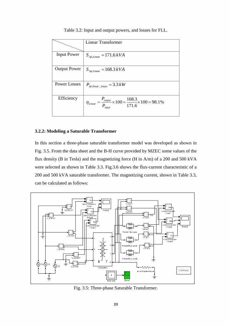
3.2.2: Modeling a Saturable Transformer

In this section a three-phase saturable transformer model was developed as shown in

Fig. 3.5. From the data sheet and the B-H curve provided by MZEC some values of the

flux density (B in Tesla) and the magnetizing force (H in A/m) of a 200 and 500 kVA

were selected as shown in Table 3.3. Fig.3.6 shows the flux-current characteristic of a

200 and 500 kVA saturable transformer. The magnetizing current, shown in Table 3.3,

can be calculated as follows:

Fig. 3.5: Three-phase Saturable Transformer.

40

max,200 ,200

max,500 ,500

,

,

:

1.7 , 10.5

1.67 , 26.24

1.8200 (1.8%) 10.5 0.189

100

1.56500 (1.56%)

100

kVA FL kVA

kVA FL kVA

m rms FL

m rms FL

from Data Sheets

B T I A

B T I A

for kVA at Normal Voltage I I A

for kVA at Normal Voltage I I

,200 ,

,500 ,

2

200

2

500

26.24 0.41

2 0.267286363

2 0.57982756

200 0.02166

500 0.02435

( ) :

1.

m kVA m rms

m kVA m rms

kVA

kVA

A

I I A

I I A

Net Cross Section Area of Core of kVA A m

Net Cross Section Area of Core of kVA A m

from B H curve

at B

7 130 /m

m m xx m

x x m

T H A m

H I HI I

H I H

Table 3.3: Magnetizing Force and Current, Induction B and Flux Ф for 200 and 500

kVA.

Magnetizing

Force H

(A/m)

Flux = B.A

( Weber)

Magnetizing

Current =

Im(Hx*Hm)

(A)

Magnetizing

Current

(pu) Flux

(pu)

500

kVA

200

kVA

500

kVA

200

kVA

500

kVA

200

kVA

500

kVA

200

kVA

0.8 0.01096 0.00975 0.00464 0.00164 0.00013 0.00011 0.26949 0.26471

10 0.01705 0.01516 0.05800 0.02056 0.00156 0.00138 0.41921 0.41176

17 0.02922 0.02599 0.09860 0.03495 0.00266 0.00235 0.71864 0.70588

20 0.03239 0.02881 0.11600 0.04112 0.00313 0.00277 0.79650 0.78235

26 0.03409 0.03032 0.15080 0.05346 0.00406 0.00360 0.83842 0.82353

100 0.04066 0.03617 0.58000 0.20562 0.01563 0.01385 1.00000 0.98235

130 0.04140 0.03682 0.75400 0.26730 0.02032 0.01800 1.01808 1.00000

300 0.04383 0.00975 1.74000 0.61685 0.04689 0.04154 1.07796 1.05882

41

Fig. 3.6: Flux-current characteristic of 200 and 500 kVA saturable transformer.

3.2.2.1: Saturation with Balanced Loads

Saturation with balanced loads and with un-balanced loads, these were tested with

three main conditions: no-load, half-load and full-load.

Case A: No-Load condition (BNL)

Same as in the no-load linear condition, but here it is for the saturable transformer

where the RL load is removed. The rms voltages and the currents of the saturable

transformer at No-load are shown in Appendix I. Fig. 3.7 shows the primary and

secondary phase voltages and currents, and the excitation current. As shown in Fig.

3.6 during the no-load condition the primary and the excitation currents are equal.

0.00000

0.20000

0.40000

0.60000

0.80000

1.00000

1.20000

0.00000 0.01000 0.02000 0.03000 0.04000 0.05000

Ma

gn

etiz

ing

Cu

rren

t, p

u

Flux, pu

200 kVA

500 kVA

42

Fig. 3.7: Voltages and currents for BNL

Case B: Half-Load (BHL)

For the half-load of the saturable transformer with 0.9 power factor lagging the RL-

load will consume 30 kW real powers and 14.5 kVAr reactive powers per phase. Table

3.4 shows the input, output powers and the efficiency of the saturable transformer,

whereas, Fig. 3.8 illustrates the voltages and currents of the primary and secondary

voltages and currents with their saturated excitation current.

43

Table 3.4: Input and output powers, the losses for BHL

Saturable Transformer

200 kVA 500 kVA

Input Power ,3 88.33inP kW

,3 87.155inP kW

Output Power ,3 87.1outP kW

,3 86.75outP kW

Efficiency 87.1100 98.61%

88.33

87.155100 99.54%

86.7

Fig. 3.8: Voltages and currents for BHL

44

Case C: Full-Load (BFL)

For the full load of the saturable transformer, the RL-load will consume 60 kW real

powers and 29 kVAr reactive powers per phase. Table 3.5 shows the input, output

powers and the efficiency whereas; Fig. 3.9 illustrates the voltages and currents of the

primary and secondary with the saturated excitation current.

Table 3.5: Input and output powers, the losses for BFL

Saturable Transformer

200 kVA 500 kVA

Input Power ,3 171.66inP kW

,3 177.55inP kW

Output Power ,3 168.6outP kW

,3 175.93outP kW

Efficiency 168.6100 98.22%

171.66

175.93100 99.1%

177.55

Fig. 3.9: Voltages and Currents for BFL

45

3.2.2.2: Saturation with Un-Balanced Linear Load

In this case, phase A - from the load side - will be fully loaded and the other two

phases B and C will consume half the load each. Table 3.6 shows the input, output

powers and the efficiency. Fig. 3.10 illustrates the phase voltages and currents of the

primary and secondary with the excitation current.

Table 3.6: Input and output powers for un-balanced linear load.

Saturable Transformer

200 kVA 500 kVA

Input Power ,3 109.75inP kW

,3 112.5inP kW

Output Power ,3 108.17outP kW

,3 111.2outP kW

Efficiency 108.17100 98.56%

109.75

111.2100 98.85%

112.5

Fig. 3.10: Voltages and Currents for un-balanced linear load.

46

3.2.2.3: Saturation with Non-Linear Load

In this case, phases A, B and C are connected to a full bridge rectifier (which

represents non-linear loads) as shown in Fig. 3.11 whereas, Fig. 3.12 illustrates the

voltages and currents for the transformer primary and secondary windings. As can be

seen from the Fig. 3.12 the current waveforms in the primary and secondary sides of

the transformers contain harmonics. The total harmonic distortion, for the secondary

current, reaches 25.46% with fundamental rms value of 262.62 A. The percentage for

each harmonic component is presented in Fig. 3.13. The percentage of harmonic

component with respect to peak rated current is depicted in Table 3.7.

Fig. 3.11: Full-Bridge rectifier load.

47

Fig. 3.12: Primary and secondary voltages and currents of the Full-Bridge rectifier

load

0

10

20

30

40

50

60

70

80

90

100

50 250 350 550 650 850 950

Figure 3.13: Current harmonic spectrum

Frequency (Hz)

Cu

rren

t (%

)

48

Table 3.7: The percentage of harmonic component with respect to peak rated current

(377.13 A).

Harmonic

Order

(h)

h2

Peak Harmonic

current (Ih)

(A)

Ih/Irated

(pu)

(Ih/Irated)2

(Ih/Irated)2 × h

2

1 1 371.45 0.985 0.97 0.9702

5 25 82.6 0.219 0.048 1.1990

7 49 34.28 0.091 0.0083 0.4058

11 121 25.35 0.067 0.0045 0.5432

13 169 13.41 0.036 0.0013 0.2190

17 289 9.66 0.026 0.00068 0.1954

19 361 5.38 0.014 0.000196 0.07076

Summation 1 3.6

According to the IEC and IEEE Standards, the load losses due to any non-sinusoidal

load currents can be calculated as follows:

2( ) ( ) ( ) (3.1)LL SLP h I R h P h

In order to make the calculation with limited data (only the manufacture certified test

report), certain assumptions have been made that are considered to be conservative.

All of the stray loss is assumed to be winding eddy-current loss.

These assumptions may be modified based on guidance from the manufacturer of the

transformer.

The load losses of the 200 kVA transformers working at full load, when feeds balance

linear load, is presented in Table 3.8.

49

Table 3.8: The load losses of the 200 kVA transformers working at full load

Load losses 3000 W

I2Req 2800 W

Eddy Current losses 200 W

If the transformer feeds non-linear load the current waveforms will contain harmonic

as presented in Fig. 3.12, the eddy current losses increases to 720 W (3.6*200) as a

result transformer efficiency will decrease.

Harmonic Filtering

In order to reduce the harmonic caused by the Full-Bridge rectifier, a 5th

and 7th

filters

are installed to mitigate the effect of the harmonics. The Total Harmonic Distortion

(THDI) is generated after running the model shown in Fig. 3.14. The parameter values

of the filters are calculated as follows and the filtered signals are shown in Fig. 3.15:

Fig. 3.14: 5th

and 7th

filters inserted to a Full-Bridge rectifier.

50

Let Quality Factor QF = 40 (because its range between (30-60))

When the P.F = 0.8 φ = cos-1

(0.8) = 36.87˚

Qold = (200 × 103) sin (36.87˚) = 120 kVAr (3.2)

If we correct the P.F to be 0.9 by adding filters, we have to get Qnew, whereas 0.9 P.F

Ө = cos-1

(0.9) = 25.842˚ (3.3)

Qnew = (200× 103) sin (25.842˚) = 87.18 kVAr (3.4)

Qneeded = 120 – 87.18 = 32.82 kVAr ≈ 33 kVAr (3.5)

The injected Q through the filters is set to be 20 kVAr for the 5th

and the 7th

order.

VL= 433 V (from the data-sheet)

ω5= 2π × 50 × 5 = 500π rad/s (3.6)

ω7= 2π × 50 × 7 = 700π rad/s (3.7)

After getting all the parameters we can calculate the capacitance, inductance and

resistance of the 5th

order and the 7th

order.

3

5 7 2 2

20 10340 / / (3.8)

. 100 (433)

QC C F phase Filter

V

C5 & C7 have the same value because they share the same reactive power & the line

voltage.

5 2 2 6

5 5

7 2 2 6

7 7

5 6

5 5

7 6

7 7

1 11.2 / / (3.9)

. (500 ) (340 10 )

1 10.61 / / (3.10)

. (700 ) (340 10 )

1 10.047 / / (3.11)

. . (500 )(340 10 )(40)

1 1

. . (700 )(340 10 )(4

F

F

L mH phase FilterC

L mH phase FilterC

R phase FilterC Q

RC Q

0.0334 / / (3.12)0)

phase Filter

51

From these parameters we have to check THDI and how it can change, if it decreases

between 6% or lower it will be a good design, if not we have to change Q or QF to get

smaller THDI.

Fig. 3.15: Voltages and currents of the filtered full-bridge rectifier.

3.3: Conclusions

From this chapter, the following points can be concluded:

The transformer parameters were obtained from the equivalent circuit of the

open circuit and short circuit tests.

Harmonics occur when non-linear loads are connected. These harmonics are

reduced by inserting designed passive shunt single-tuned filters. The dominant

harmonics were the 5th

and the 7th

for 200 kVA and 500 kVA for the full-

bridge rectifier load.

Transformer efficiency was calculated at different load conditions.

The maximum efficiency occurs at about half of the load.

52

Chapter 4: Transformer Efficiency

4.1: Introduction

The power efficiency is simply defined as the ratio of the output power to the input

power. In any electrical equipment, the efficiency never reaches 100% because of

losses. In practical transformer the losses can be classified as shown in Fig. 4.1.

Fig. 4.1: Transformer Losses.

1) No-Load Losses (iron losses): The iron losses happen whenever the transformer is

energized and the amount of these losses is dependent on the excitation voltage of the

transformer [30]. The iron losses are consisting of hysteresis losses and eddy losses.

Hysteresis losses are due to elementary magnets in the material aligning with the

alternating magnetic field [31]. In addition, the hysteresis losses comprise about three

fourths of the total of the core losses [32]. Eddy currents losses due to the alternating

magnetic field. The kind of the core material is very important factor in reducing core

losses, because different types of the core materials have different magnetizing

characteristics. Equations 4.1 and 4.2 are used to calculate the eddy current and

hysteresis losses respectively.

Transformer total losses

No Load

Hysteresis

loss

Eddy loss

(PEC )

Load

Stray loss

(PSL)

Winding eddy loss

Other stray loss (POSL)

Windings

loss(I2R)

53

2 2 2

1

2

. . . (4.1)

. . (4.2)

e rms

n

h mp

P K f t B

P K f B

where,

f : is the frequency.

t : is thickness of individual lamination.

K1 and K2 : are constants which depend on material.

Brms : is the rated effective flux density corresponding to the actual r.m.s. voltage on

the sine wave basis.

Bmp : is the actual peak value of the flux density.

n : is the Steinmetz constant having a value of 1.6 to 2.0 for hot rolled laminations and

a value of more than 2.0 for cold rolled laminations due to use of higher operating flux

density in them[33].

2) Load Losses: The load losses are more significant source of heat in the transformer

than the no-load losses [31]. This kind of losses can be divided into copper loss (I2R)

and stray load loss (PSL).

The (I2R) is caused by winding resistance and it is proportional to the square of the

load current multiply by winding resistance [30].The (PSL) is due to electromagnetic

field in the winding, core clamps, magnetic shields, tank walls, etc... The stray loss is

subdivided into winding eddy loss and structural parts stray loss (POSL). The winding

eddy loss (PEC) is the result of eddy and circulation current losses. The other structures'

loss except the windings like clamps, tank walls, etc..; are grouped under the stray

loss. The load losses (PLL) can be computed by:

PLL = I2R + PEC + PSL (4.3)

The transformer operates at maximum efficiency when the core loss equal to the

cupper loss. Fig. 4.2 shows the percent load vs. power loss for 200 kVA and 500 kVA

distribution transformer.

54

Fig. 4.2: Power Loss vs. Percent Load.

4.2: Matlab Simulation for 200kVA and 500kVA Distribution Transformer

200 kVA distribution transformer are modeled by MATLAB, the model is presented in

Appendix J, in this model different load and power factor was taken in consideration.

Table 3.1 shows the transformer parameters which were used in the MATLAB model.

Fig. 4.3 represents the MATLAB simulation result for 200kVA and 500kVA

efficiencies, the x-axis is scaled up 150% because the distribution transformers are

usually overloaded.

Fig. 4.3: Power Efficiency Curves for 200kVA and 500kVA Distribution

Transformer at Different Load Power Factors.

55

Table 4.1: Maximum Efficiency vs. Power Factor of 200kVA and 500kVA

Distribution Transformer.

Load (%) Efficiency (%)

500kVA 200kVA 500kVA 200kVA P.F (Lagging)

48.32 40.27 98.81 98.27 0.7

48.32 40.27 98.93 98.48 0.8

48.32 40.27 99.08 98.66 0.9

48.32 40.27 99.16 98.81 1

4.3: All Day Efficiency

The power transformers usually operate at its full capacity so that‟s way they are

designed to have maximum efficiency at their rated output. The distribution

transformer are operated below its rated output power for the most of the time, so the

manufacturer design the distribution transformer to have the maximum efficiency

between [40% - 50%] of its rated output [34]. Matlab code in Appendix K was used to

determine the full day efficiency and the loss energy cost in $ for any load profile.

4.3.1: Case Study

The MATLAB show the efficiency over full day and then calculate the average

efficiency. Also MATLAB calculate the 24-hours‟s energy cost assuming the cost per

kWh is 0.10$ as shown in Table 4.2.

Table 4.2: 24- hour energy cost

Calculated value of full day efficiency, ηAD = 98.42%

% LOAD 50 60 55 65 70

P.F 0.8 0.8 0.85 0.87 0.84

HOURS 3 5 5 4 7

56

0 5 10 15 20 25100

110

120

130

140Power load profile

Load

, kW

Time, hr

0 5 10 15 20 2598

98.2

98.4

98.6Effieiency profile

Effic

ienc

y, %

Time, hr

4.3.1.1: MATLAB Result

24-All-Day Efficiency (%) - 98.3%

Hour-Energy cost 5.1551$ kW/hr

Fig. 4.4: Loads and Efficiency Profile for 200 kVA.

There is small difference between the results calculated and MATLAB result because

MATLAB considers the losses due to the primary, secondary and the core resistances.

4.4: Conclusions

From this chapter, it can be concluded the following:

The maximum efficiency of the distribution transformer lies within [40% -

50%] in general, because the transformers usually operate below its rated

output power.

The iron losses happen whenever the transformer is energized and the amount

of these losses is dependent on the excitation voltage of the transformer.

The load losses are more significant source of heat in the transformer than the

no-load losses.

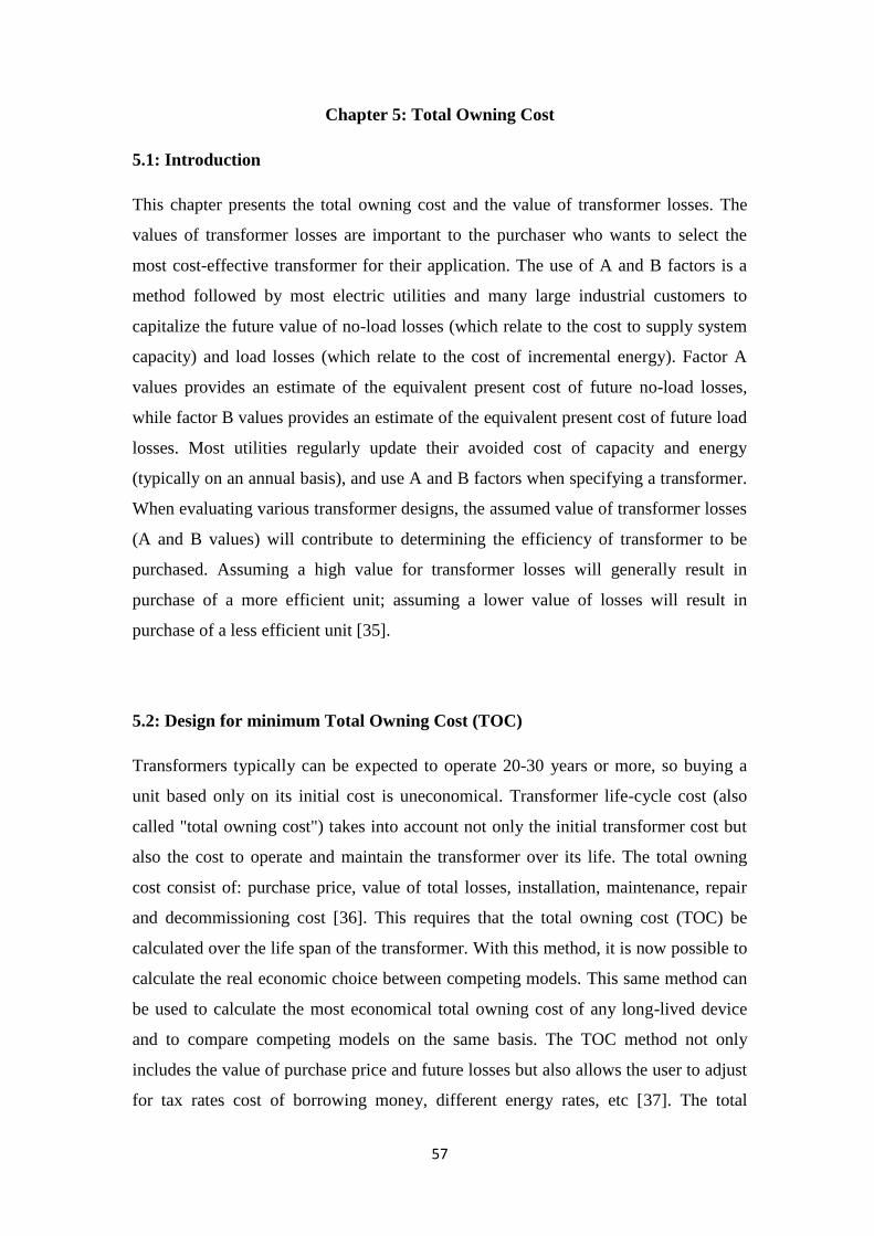
57

Chapter 5: Total Owning Cost

5.1: Introduction

This chapter presents the total owning cost and the value of transformer losses. The

values of transformer losses are important to the purchaser who wants to select the

most cost-effective transformer for their application. The use of A and B factors is a

method followed by most electric utilities and many large industrial customers to

capitalize the future value of no-load losses (which relate to the cost to supply system

capacity) and load losses (which relate to the cost of incremental energy). Factor A

values provides an estimate of the equivalent present cost of future no-load losses,

while factor B values provides an estimate of the equivalent present cost of future load

losses. Most utilities regularly update their avoided cost of capacity and energy

(typically on an annual basis), and use A and B factors when specifying a transformer.

When evaluating various transformer designs, the assumed value of transformer losses

(A and B values) will contribute to determining the efficiency of transformer to be

purchased. Assuming a high value for transformer losses will generally result in

purchase of a more efficient unit; assuming a lower value of losses will result in

purchase of a less efficient unit [35].

5.2: Design for minimum Total Owning Cost (TOC)

Transformers typically can be expected to operate 20-30 years or more, so buying a

unit based only on its initial cost is uneconomical. Transformer life-cycle cost (also

called "total owning cost") takes into account not only the initial transformer cost but

also the cost to operate and maintain the transformer over its life. The total owning

cost consist of: purchase price, value of total losses, installation, maintenance, repair

and decommissioning cost [36]. This requires that the total owning cost (TOC) be

calculated over the life span of the transformer. With this method, it is now possible to

calculate the real economic choice between competing models. This same method can

be used to calculate the most economical total owning cost of any long-lived device

and to compare competing models on the same basis. The TOC method not only

includes the value of purchase price and future losses but also allows the user to adjust

for tax rates cost of borrowing money, different energy rates, etc [37]. The total

58

owning cost (TOC) method provides an effective way to evaluate various transformer

initial purchase prices and cost of losses. The goal is to choose a transformer that

meets specifications and simultaneously has the lowest TOC.The utility engineers

traditionally determine whether an energy efficient transformers is cost effective by

calculating the values of the no load and load losses. These are often referred to as the

"A" and "B" factors. They are multiplied by no load and load losses respectively and

applied to the total owning cost (TOC) formula given by [35],

TOC = NLL × A+ LL × B + C (5.1)

where,

TOC: capitalized total owning cost,

NLL: the no load loss in kW,

A: the capitalized cost per rated kW of NLL (no load loss factor in $/W),

LL: transformer load losses,

B: the capitalized cost per rated kW of LL (load loss factor in $/W),

C: the initial cost of the transformer including transportation, sales tax, and other costs

to prepare it for service. Among all transformer offers, the most cost-effective and

energy-efficient transformer is the one with the lowest TOC. Since the formula

includes the cost of losses, which will occur in the future, it is necessary to discount

these future costs to equate them to present-day dollars. The transformer manufacturer

supplies the bid price. If the A and B factors are known, then the manufacturers should

base the bid prices on the same A and B factors in all cases. The purchase price and

the energy losses are the two key factors in comparing and specifying different

transformers. When transformers are compared with respect to energy losses, the

process is called loss evaluation and the A and B parameters are known as loss

evaluation factors [38].

59

5.3: Specifying A and B Values

For custom-designed transformers, manufacturers optimize the design of the unit to

the specified A and B values resulting in a transformer designed to the lowest total

owning cost, rather than one designed for cheapest first cost. In situations where A

and B values have not been determined (or the enduser does not utilize or specify

them), such as occur in commercial or small industrial applications, the suggested

technique to maximize transformer efficiency is to obtain the no-load and full-load

loss values of a specific transformer, in watts. We can calculate the value of A & B

using "probabilistic approach", when we calculate the value of A and B, we can

calculate the total owning cost as it shown in Fig. 5.1.

Fig. 5.1: Transformer LCC Spreadsheet Model Flowchart.

60

5.3.1: Probabilistic Approach

In this method the no load loss factor A and load loss factor B values are submitted to

the transformer manufacturers on a request for quotation. The manufacturer then

designs a distribution transformer in response to the price offer by utilizing a

combination of different materials so it could come to the optimum TOC price to

obtain the order [39].

The factors A & B are computed using this formula:

(1 ) 1

(1 )

n

KWhn

iA C HPY

i i

(5.2)

2(1 ) 1( )

(1 )

n

lKWhn

r

IiB C HPY

i i I

(5.3)

where,

i : interest rate.

n: lifetime in years ( for 25 years n = 25), this value is obtained from Mazoon

Electricity Company.

KWhC : kWh price in OMR/kWh or in $/kWh = 0.03 OMR/kWh

HPY: number of hours in a year that the transformer is connected to the power grid,

which is 8760 h /year

lI : Loading current

rI : Rated current

We got all the parameters except the loading current, and the interest rate, so we try to

take several values, and assume some values. So, we find a relation between factor

“A”, and the interest rate (n) along the life time, as it shown in Fig. 5.2.

61

Fig. 5.2: The relation between A and n along life time.

Fig. 5.2 shows that whenever we decrease the interest rate, we the value of A increase,

which will effect on the value of B, and then increase the total owning cost (TOC), so,

we have to select the highest interest rate.

The second parameter is the loading current, which is varying from hour to hour, but

we try to take the average of the loading current annually, for three different years by

taking the area under the curve, to calculate the average loading current as it shown in

Fig. 5.3.

Fig. 5.3: The loading current annually for three years.

0

500

1000

1500

2000

2500

3000

3500

4000

4500

5000

0 5 10 15 20 25 30

Fact

or

A (

O.M

.R/k

W)

Life time (years)

The Relation Between A,n and i

3%

4%

5%

6%

7%

8%

9%

10%

11%

12%

0

20

40

60

80

100

120

1 2 3 4 5 6 7 8 9 10 11 12

Load

ing

curr

en

t (%

)

Months

Loading current 2003

Loading current 2004

Loading current 2005

62

Fig. 5.3 shows the loading current for a year, to calculate the average of the loading

current, we calculate the area under the curve, and we can calculate the peak load and

the load factor:

For 2003:

Average loading current = 0.57= 57% (By calculating the area under the curve)

Peak load = 80 %

Load Factor ( LDF )= 7125.080.0

57.0

LoadPeak

LoadAveragep.u

For 2004:

Average loading current = 0.67 = 67 %

Peak load = 90 %

Load Factor = 7444.090.0

67.0

LoadPeak

LoadAveragep.u

For 2005:

Average loading current = 0.77 = 77 %

Peak load = 100 %

Load Factor = 77.000.1

77.0

LoadPeak

LoadAveragep.u.

If we select the loading current which was in 2003, we can calculate the total owning

cost, by calculating the value of B, as we mention before the value of B is varying

according to the loading current, unlike the value A. We notice that the value of A is

constant and doesn‟t vary with the change in the loading current. We can compute the

value of B now, because B = A2)(

r

l

I

I [25].

63

Fig. 5.4: The relation between A & B.

Fig. 5.4 shows the relation between A and B, the value of A is constant and doesn‟t

vary with the change in the loading current, but the value of B is changing according

to the loading current of a distribution of transformer. If the current increases, the cost

of load losses (B) increase, but when the transformer is working during full load that

means )(r

l

I

I=100%, the load losses cost (B) = no load losses cost (A).

If we want to calculate the total owning cost of 200 kVA, we find the value of A & B.

By assuming interest rate of 3% (by taking the smallest interest rate), and taking the

average loading current for 2003 which is 0.57.

25

25

(1 0.03) 10.03 8760 4576.17( / ) 4.57617 ( / )

0.03(1 0.03)A OMR kW OMR W

2574576.17 ( ) 1486.8 ( / ) 1.4868 ( / )

100B OMR kW OMR W

By taking the value of no load loss, load loss and initial cost which is given from the

data sheet of Mazoon Electricity Company, as shown in Table 5.1, the total owning

cost can be calculated.

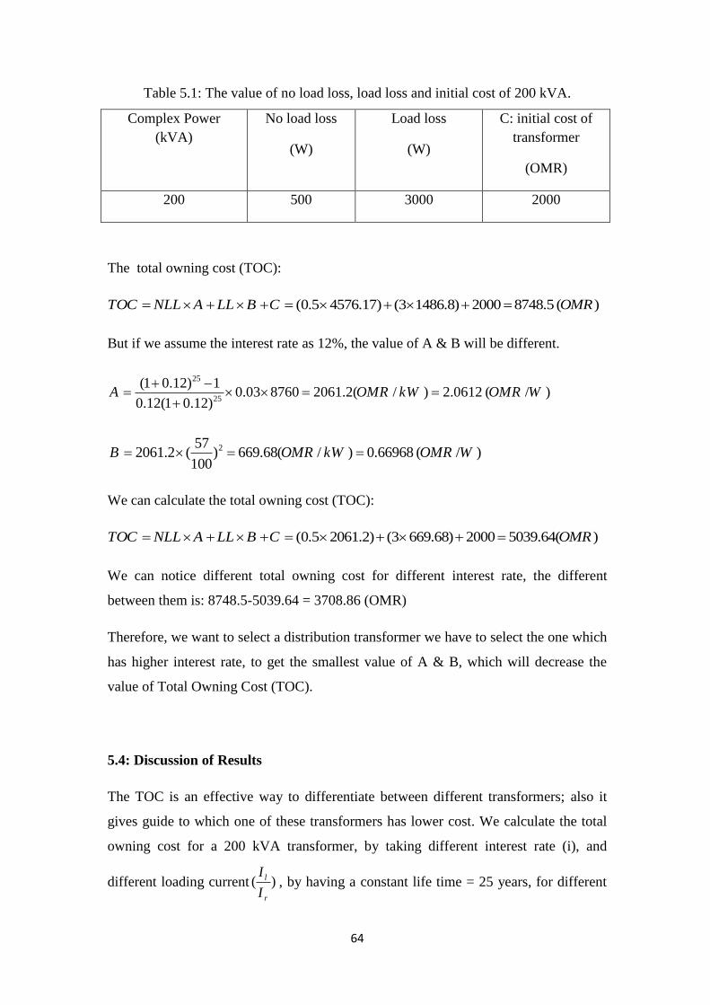
64

Table 5.1: The value of no load loss, load loss and initial cost of 200 kVA.

Complex Power

(kVA)

No load loss

(W)

Load loss

(W)

C: initial cost of

transformer

(OMR)

200 500 3000 2000

The total owning cost (TOC):

(0.5 4576.17) (3 1486.8) 2000 8748.5 ( )TOC NLL A LL B C OMR

But if we assume the interest rate as 12%, the value of A & B will be different.

25

25

(1 0.12) 10.03 8760 2061.2( / ) 2.0612 ( / )

0.12(1 0.12)A OMR kW OMR W

2572061.2 ( ) 669.68( / ) 0.66968 ( / )

100B OMR kW OMR W

We can calculate the total owning cost (TOC):

(0.5 2061.2) (3 669.68) 2000 5039.64( )TOC NLL A LL B C OMR

We can notice different total owning cost for different interest rate, the different

between them is: 8748.5-5039.64 = 3708.86 (OMR)

Therefore, we want to select a distribution transformer we have to select the one which

has higher interest rate, to get the smallest value of A & B, which will decrease the

value of Total Owning Cost (TOC).

5.4: Discussion of Results

The TOC is an effective way to differentiate between different transformers; also it

gives guide to which one of these transformers has lower cost. We calculate the total

owning cost for a 200 kVA transformer, by taking different interest rate (i), and

different loading current )(r

l

I

I, by having a constant life time = 25 years, for different

65

years. Fig. 5.5 shows the relation between the total owning cost, and the interest rate

by taking random interest rate (3%, 6%, 9%, 12%), for three different years (2003,

2004, 2005) to notice the different between them.

Fig. 5.5: The total owning cost vs. the interest rate.

Fig. 5.5 shows the total owning cost for different interest rate and different loading

current, we notice from the figure that the maximum total owning cost occurs at 2005

at 3% interest rate, because of having high loading current 77%, whereas the minimum

total owning cost occurs at 2003 at 12 % interest rate, because of having low loading

current 57%. So, whenever we want to buy a trasnformer we have to select the one

which has a higher interest rate, and lower loading current. But if we have two

transformers with the same initial cost 2000 OMR, how can I choose the best

transformer? An example is made and shown in Appendix L.

The factors A and B which have been calculated using probabilistic method, is a

very sensitive factors, the factor A is proportional to the energy cost ( KWhC ) and life

time (n), but has an inverse proportional to the interest rate (i), the factor B is

proportional to the energy cost ( KWhC ), life time (n), and load ratio )(r

l

I

I, but has an

inverse proportional to the interest rate (i). Therefore, one of the main goals of the

3% 6% 9% 12%

2003 8748.5 6954.2 5806.5 5039.64

2004 10450.745 8203.913 6767.1 5806.41

2005 12427.7 9655.21 7882.177 6696.85

0

2000

4000

6000

8000

10000

12000

14000

Tota

l ow

nin

g co

st (

O.M

.R)

66

country's energy sector is optimizing electric energy consumption by considering

transformer losses cost during its lifetime and utilizing more efficient distribution

transformers.

5.5 Conclusion

The total owning cost is one of the most important factors that the company

should consider when buying transformers.

The total owning cost depends on the value of A and B.

The value of A is varying according to the interest rate, life time, and the ratio

of price per kWh. It doesn‟t vary with the varying in the loading current.

The value of B is varying according to the same parameters of A, but it

depends on the change of the loading current.

Heat losses reduce the life time of a transformer by causing damage to the

insulation over a long time, which will cause the transformer to fail.

The best transformer is the one with lower total owning cost, longer life, lower

losses and lower failure rate.

The total owning cost method provides an effective way to evaluate various

transformer initial purchase prices and cost of losses.

We care about the interest rate because it‟s the only parameter that could affect

the total owning cost, since the loading current is varying annually from year to

year, so we can't control it.

When we want to select a transformer we choose the one which has the lower

(TOC), by having higher interest rate and lower loading current, because the

transformer will have lower losses and lives more, which is more economical

for the company.

67

Chapter 6: Conclusions

6.1: Summary

From our survey and simulation we conclude

Transformers are classified according to their size, insulation, cooling method

and location. The main parts of the transformer are windings, core, insulators,

tank and the bushing.

Cores are usually made of silicon steel but recently the manufacturers use

amorphous iron because of its lower eddy current losses and narrow hysteresis

loop.

Transformers are classified according to their size, insulation, cooling method

and location. The main parts of the transformer are windings, core, insulators,

tank and the bushing.

Cores are usually made of silicon steel but recently the manufacturers use

amorphous iron because of its lower eddy current losses and narrow hysteresis

loop.

The transformer parameters were obtained from the equivalent circuit of the

open circuit and short circuit tests.

Harmonics occur when non-linear loads are connected. These harmonics are

reduced by inserting designed passive shunt single-tuned filters. The dominant

harmonics were the 5th

and the 7th

for 200 kVA and 500 kVA for the full-

bridge rectifier load.

The maximum efficiency of the distribution transformer lies within [40% -

50%] in general, because the transformers usually operate below its rated

output power.

The best transformer is the one with lower total owning cost, longer life, lower

losses and lower failure rate.

The total owning cost is one of the most important factors that the company

should consider when buying transformers.

When we want to select a transformer we choose the one which has the lower

(TOC), by having higher interest rate and lower loading current, because the

transformer will have lower losses and lives more, which is more economical

for the company.

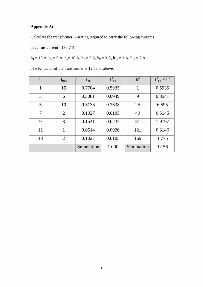
I

Appendix A:

Calculate the transformer K-Rating required to carry the following currents

True rms current =19.47 A

h1 = 15 A, h3 = 6 A, h5= 10 A, h7 = 2 A, h9 = 3 A, h11 = 1 A, h13 = 2 A

The K- factor of the transformer is 12.56 or above.

I2

pu × h2 h

2 I

2pu Ipu Irms h

0.5935 1 0.5935 0.7704 15 1

0.8541 9 0.0949 0.3081 6 3

6.595 25 0.2638 0.5136 10 5

0.5145 49 0.0105 0.1027 2 7

1.9197 81 0.0237 0.1541 3 9

0.3146 121 0.0026 0.0514 1 11

1.775 169 0.0105 0.1027 2 13

12.56 Summation 1.000 Summation

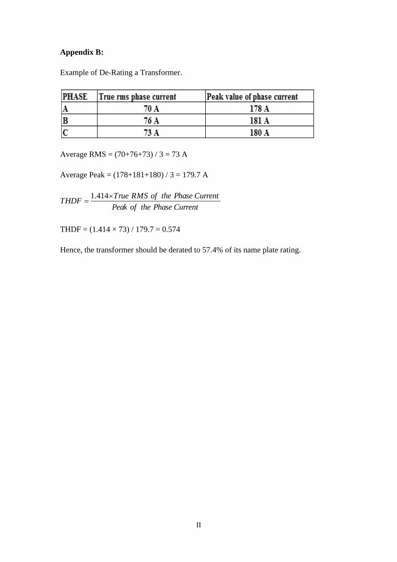
II

Appendix B:

Example of De-Rating a Transformer.

Average RMS = (70+76+73) / 3 = 73 A

Average Peak = (178+181+180) / 3 = 179.7 A

1.414 True RMS of the Phase CurrentTHDF

Peak of the Phase Current

THDF = (1.414 × 73) / 179.7 = 0.574

Hence, the transformer should be derated to 57.4% of its name plate rating.

III

Appendix C.1: Data-Sheet for 200 kVA

IV

V

VI

VII

Appendix C.2: Data-Sheet for 500 kVA

VIII

IX

X

XI

Appendix D: MATLAB model that calculates the parameters of the transformer

%----------------------------------------------------------

% Program that calculates the parameters of a transformer--

%----------------------------------------------------------

% Set the value of the primary voltage and number of turns.

V1= 11e3;

V2= 433;

V2p=433/sqrt(3);

N= V1/V2p;

% Set the value of the real power(per phase).

P1= (500)/3;

% getting the primary and the phase current.

I1= (1.8*10.5)/100;

Ip= I1/(sqrt(3));

% Getting the angle.

pf= acosd(P1/(V1*Ip));

% for the magnetizing current.

Ic= Ip*(cosd(pf));

Im= Ip*(sind(pf));

% getting the values of the magnetizing part.

Rc= V1/Ic;

Xm= V1/Im;

% setting the secondary current.

I2= 0.42;

P2= 1000/3;

% getting the R-equivalent from copper power(losses).

Pc= 3000;

I11= 10.5;

I11p= 10.5/sqrt(3);

Req= Pc/(3*(I11p^2));

Zeq= ((4.75/100)*V1)/I11p;

Xeq= sqrt((Zeq^2)-(Req^2));

% given stator resistance (R1) we get the (R2')

R1= 14.75;

R21= Req-R1;

R22= R21/(N^2);

X1= (Xeq/2);

X21= (Xeq/2);

XII

Appendix E: The Open-Circuit Test:

In this test we leave one side of the transformer open circuited, while to the other we apply

the rated voltage and measure the current and the power. On the open circuited side of the

transformer (usually Low-Voltage winding is supplied, while High-Voltage is kept open for

ease of testing and availability of supply), the rated voltage appears and the current that flows

is primarily determined by the impedances cm RandX , and it is much lower than rated. We

will use these two measurements to calculate the values of cm RandX . The power in the

Open-Circuit Test consists of Core loss and primary winding ohmic loss, but we neglect the

winding loss because it is very small comparing with the Core loss [27-30]. Fig. B.1 shows

the simplified equivalent circuit for applying the Open-Circuit Test. Also there are several

calculations regarding the test to get the cm RandX :-

Fig. E: Open-Circuit Test

m

m

cc

cc

oom

ooc

cmo

o

co

ooc

I

VX

P

V

I

PR

II

II

III

IV

P

IVP

1

2

1

2

1

1

sin

cos

cos

cos

Where:-

cP : No-Load (Core Loss).

:1V Rated voltage.

oI : No-Load Current.

cm II , : Magnetizing and core loss

components respectively.

ocos : No-Load Power Factor

cm RX , : Shunt Branch Parameters

XIII

Appendix F: The Short-Circuit Test:

In this test we short circuit one side of the transformer and apply the rated

current to the other. We measure the voltage of that side and the power drawn.

On the other side, (the Short-Circuited one) the voltage is of course zero, but the

current is rated the figure of the Short-Circuit Test is shown in Fig. C.1 [27-30].

Also there are some calculations involved in finding the rest of the parameters:-

Fig. F: Short-Circuit Test

eqeqeq

SC

Leq

SC

SCeq

RZX

I

PR

I

VZ

22

2

In order to get the parameters of the transformers, a simple model using

MATLAB with the help of the above rules and calculations is designed and the

results obtained are shown in Table 3.1.

Where:-

LP : Load Loss (iron Loss).

eqR ,eqX : Equivalent circuit

parameters.

XIV

Appendix G: Values of all currents and voltages of linear transformer for

NLL

VV_source1 = 6350.85 Vrms 0.00°

I_source1 = 0.19 Arms -82.09°

V_load1 = 249.88 Vrms 30.00°

I_load1 = 0.00 Arms 0.00°

Ub: Series RLC Load = 0.00 Vrms 0.00°

Ib: Series RLC Load = 0.00 Arms 0.00°

Uab_w1: Transformer = 11000.00 Vrms 30.00°

Ubc_w1: Transformer = 11000.00 Vrms 150.00°

Uca_w1: Transformer = 11000.00 Vrms -90.00°

Iab_w1: Transformer = 0.11 Arms -52.09°

Ibc_w1: Transformer = 0.11 Arms 67.91°

Ica_w1: Transformer = 0.11 Arms -172.09°

Uan_w2: Transformer = 249.88 Vrms 30.00°

Ubn_w2: Transformer = 249.88 Vrms 150.00°

Ucn_w2: Transformer = 249.88 Vrms -90.00°

Ian_w2: Transformer = 0.00 Arms 0.00°

Ibn_w2: Transformer = 0.00 Arms 0.00°

Icn_w2: Transformer = 0.00 Arms 0.00°

Imag_A: Transformer = 0.11 Arms -52.09°

Imag_B: Transformer = 0.11 Arms 67.91°

Imag_C: Transformer = 0.11 Arms -172.09°

SOURCES:

V3 = 6350.85 Vrms -120.00°

V2 = 6350.85 Vrms 120.00°

V1 = 6350.85 Vrms 0.00°

XV

Appendix H: Values of all currents and voltages of linear transformer for

FLL

V_source1 = 6350.85 Vrms 0.00°

I_source1 = 10.23 Arms -39.16°

V_load1 = 240.46 Vrms 28.44°

I_load1 = 256.51 Arms -8.43°

Ub: Series RLC Load = 240.46 Vrms 28.44°

Ub: Series RLC Load1 = 240.46 Vrms 148.44°

Ub: Series RLC Load2 = 240.46 Vrms -91.56°

Ib: Series RLC Load = 256.51 Arms -8.43°

Ib: Series RLC Load1 = 256.51 Arms 111.57°

Ib: Series RLC Load2 = 256.51 Arms -128.43°

Uab_w1: Transformer = 11000.00 Vrms 30.00°

Ubc_w1: Transformer = 11000.00 Vrms 150.00°

Uca_w1: Transformer = 11000.00 Vrms -90.00°

Iab_w1: Transformer = 5.91 Arms -9.16°

Ibc_w1: Transformer = 5.91 Arms 110.84°

Ica_w1: Transformer = 5.91 Arms -129.16°

Uan_w2: Transformer = 240.46 Vrms 28.44°

Ubn_w2: Transformer = 240.46 Vrms 148.44°

Ucn_w2: Transformer = 240.46 Vrms -91.56°

Ian_w2: Transformer = 256.51 Arms 171.57°

Ibn_w2: Transformer = 256.51 Arms -68.43°

Icn_w2: Transformer = 256.51 Arms 51.57°

Imag_A: Transformer = 0.11 Arms -52.83°

Imag_B: Transformer = 0.11 Arms 67.17°

Imag_C: Transformer = 0.11 Arms -172.83°

SOURCES:

V3 = 6350.85 Vrms -120.00°

V2 = 6350.85 Vrms 120.00°

V1 = 6350.85 Vrms 0.00°

XVI

Appendix I: Values of all currents and voltages of Saturable transformer

for NLS

V_source1 = 6350.85 Vrms 0.00°

I_source1 = 0.03 Arms -0.00°

V_load1 = 249.99 Vrms 30.00°

I_load1 = 0.00 Arms 0.00°

Ub: Series RL Load = 0.00 Vrms 0.00°

Uab_w1: Transformer = 11000.00 Vrms 30.00°

Ubc_w1: Transformer = 11000.00 Vrms 150.00°

Uca_w1: Transformer = 11000.00 Vrms -90.00°

Uan_w2: Transformer = 249.99 Vrms 30.00°

Ubn_w2: Transformer = 249.99 Vrms 150.00°

Ucn_w2: Transformer = 249.99 Vrms -90.00°

Ib: Series RL Load = 0.00 Arms 0.00°

Iab_w1: Transformer = 0.02 Arms 30.00°

Ibc_w1: Transformer = 0.02 Arms 150.00°

Ica_w1: Transformer = 0.02 Arms -90.00°

Ian_w2: Transformer = 0.00 Arms 0.00°

Ibn_w2: Transformer = 0.00 Arms 0.00°

Icn_w2: Transformer = 0.00 Arms 0.00°

Imag_A: Transformer = 0.00 Arms 0.00°

Imag_B: Transformer = 0.00 Arms 0.00°

Imag_C: Transformer = 0.00 Arms 0.00°

SOURCES:

V3 = 6350.85 Vrms -120.00°

V2 = 6350.85 Vrms 120.00°

V1 = 6350.85 Vrms 0.00°

XVII

Appendix J: MATLAB Code for 200KVA to find its Efficiency:

The same code is used for 500KVA except that the values of Table 4.3 were

used.

XVIII

Appendix K: MATLAB Code for 200KVA to find its Full-Day Efficiency

The same code is used for 500KVA except that the values of Table 4.3 were

used.

XIX

Appendix L: Case Study of TOC

We have two transformers of (200 kVA), with a same initial cost (2000 OMR), and the

same interest rate (i=18%) but they have different life time (n), for transformer 1

(n=25), for transformer 2 (n=30).

Question: Which transformer is better more economical?

Answer:

For transformer 1:

A = 25

25

(1 0.18) 10.03 8760 1436.7( / )

0.18(1 0.18)OMR kW

B = A2)(

r

l

I

I = 250

1436.7 ( ) 359.2( / )100

OMR kW

TOC = NLL*A+ LL*B + C

= (0.5 1436.7) (0.75 359.2) 2000 2987.75( ) 3000( )OMR OMR

For transformer 2:

A = 30

30

(1 0.18) 10.03 8760 1450( / )

0.18(1 0.18)OMR kW

B = A2)(

r

l

I

I =

2501450 ( ) 362.45( / )

100OMR kW

TOC = NLL × A+ LL × B + C

= (0.5 145) (0.75 36.245) 2000 2997( ) 3000OMR

We notice that transformer one and transformer two have approximately equals total

owning cost, but transformer two is the best, because it can live more than transformer

one for about five years, which means that is more economical for the company.

XX

Appendix M: FYP Proposal

XXI

XXII

References:

[1] Laplante P.A., Electrical engineering dictionary (CRC, 2000).

[2] P.C.SEN, Principle of Electric Machines and Power Electronics, Second

Edition .1997

[3] TRANSFORMERS AND REGULATORS, chapter 7

<URL:http://www.usace.army.mil/publications/armytm/tm5-

684/chap7.pdf>

[4] <URL:http://www.eas.asu.edu/~karady/360_stuff/Lectures/

Lecture%209%20Mag%Circuit-Transformrts.ppt>

[5] Stephen J.Chapman, Electric Machinery Fundamentals, Formerly of the

University of Houston, 1985 by McGraw Hill Book Company.

[6] <URL: http://www.sayedsaad.com>

[7] John Hindmarsh, Electrical Machines and their Applications, (4th

edition), Senior Lecturer at the University of Mancherster Instate.

[8] George McPherson, Robert, D. Laramore, An Introduction to Electrical

Machines and Transformer, 1990 by John Wiley and Sons.

[9] <URL:http://library.abb.com/GLOBAL/SCOT/scot252.nsf/VerityDisplay/

ED2F8B0D60C51F48C1256BEB004190F2/$File/1ZSE%202750-

107%20en%20Rev%201.pdf>

[10] “Power Quality and Utilisation Guide, On Line Diagnostic Monitoring

for Large Power Transformers”, Angelo Baggini University of Bergamo,

Franco Bua, Engineering Consulting & Design February 2008.

[11] Investigating transformer failures by William Barthley. Hartford Steam

Boiler Inspection & Insurance Co. Hartford, CT

<URL:http://www.omicron.at/en/products/app/power-

transformer/transformer- moisture/>

[12] EGS Electrical Group

<URL: www.solaheviduty.com>

[13] <URL: http://www.springerlink.com/content/2p7bwlbtt4htq4qb/ >

"Reactive load control of parallel transformer operations using neutral

networks” Fakhur Islam, Baikunth Nath and Joarder Kamruzzaman

[14] "Electric Machines I " Prof. Krishna Vasudevan, Prof. G. Sridhara Rao,

XXIII

Prof. P. Sasidhara Rao.

[15] <URL:http://www.patentstorm.us/patents/5369388/description.html.>

[16] Grounding Power Distribution System, Jim Phillips ,P.E, April 2005

[17] Practical Grounding of Utility and Industrial Distribution Systems.

IDC Technologies.

[18] Practical Power System Protection, Mark Brown, Ben Ramesh,

2004.

[19] “Power Quality Application Giude, Harmonics Selection and Rating of

Transfromers”. Prof Jan Desmet, Hogeschool West-Vlaanderen

&Gregory

Delaere, Labo Lemcko. November 2005

[20] “Power System Harmonics”, Jos Arrillaga and Neville R.Waston,

University of Canterbury, Christchurch, Newzealand. Second edition

2004.

[21] “Power Quality”, C. SANKARAN. CRC Press 2001

[22] “Electrical Power System Quality”, Second Edition. Roger C.Dugan,

Mark F. Mcgranaghan, Surya Santoso and H.Wayna Beaty. 2002

[23] “Survay of Harmonics Measurments in Electrical Distribution System”.

Leon M. Tolber, member in IEEE. Harold D. Hollis and Peyton S.Hale

[24] “Intrapting The National Electric Code”. Truman C. Surbrook and

Jonathan R. Althouse. 7th edition

[25] “Harmonics in Low Voltage Three-Phase Four-Wire Electric

Distribution Systems and Filtering Solutions”. Dr. Prasad Enjeti Texas

A&M University Power Electronics and Power Quality Laboratory.

[26] “The Power Electronic Handbook, Industrial Electronics Series”.

Timothy L. Skvarenina. CRC Press 2002.

[27] “Analysis of Zig-Zag Transformer Applying in the Three-Phase Four-

Wire Distribution Power System”, Hurng-Liahng Jou, Member, IEEE,

Jinn-Chang Wu, Kuen-Der Wu, Wen-Jung Chiang, and Yi-Hsun Chen

[28] “A New Approach of Distribution System Reconfiguration for Loss

Minimization”, M.A. Kashem, G.B. Jasmon, V. Ganapathy

XXIV

[29] MATLAB HELP

<URL:http://www.mathworks.com/products/simpower/>

<URL:http://www.mathworks.com/products/simulink/>

[30] Martin J.Heathcote, CEng, FIEE, The J&P Transformer Book, (12th

Edition).

[31] Rich Hunt, M.S, P.E , Michael L, Giordano B.S, P.E " Thermal Overload

Protection of Power Transformer Operating Theory and Practical

Experience ", 59th Annual Protective Relaying Conference, Georgia

Tech,, Atlanta, Georgia, April 27th– 29th ,2005.

[32] <URL:

http://ourworld.compuserve.com/homepages/boyce_smith/action.html>

[33] Transformer Engineering, Designing and practice, S.V.Kulkarni,

S.A.Khaparde, Indian

Institute of Technology, Bombay, Mumbai, India

[34] Jimmie J. Cathey, Mc Graw Hill., Electricmachines Analysis and Design

Appling Matlab

[35] <URL:

http://www.copper.org/applications/electrical/energy/trans_losses.html>

[36] <URL:http://www.leonardo-energy.org/transformers/Files/PL-9.pdf>

[37] <URL:

http://www.copper.org/applications/electrical/energy/trans_life_cycle.ht

ml>

[38] H. D. Keulenar, D. Chapman, and S. Fassbinder, “The Scope for Energy

Saving in the EU Through the Use of Energy Efficient Electricity

Distribution Transformers,” Proc. of IEE Conf. CIRED2001, No. 482, P.

4.27, 2001.

[39] S. Bouwman, J. F. Groeman, and W. T. J. Hulshorst, Cost Savings by

Low-loss Distribution Transformers. KEMA Netherland B.V.

Report, by Order of European Copper Institute, 38 Pages, 2003.

[40] Ali Arzani and Ehsan Dabbagh, "Loss Evaluation of Distribution

Transformers in Iran's Electric Power System" Industrial

Applications of Energy Systems Systems ( IAES2008 )

PROCEEDINGS Sohar University Sultanate of Oman, April 1-2, 2008