Prototype and Metrics for Data Processing Chain Components of IPM

Vuong Ly

HyspIRI SymposiumIntelligent Payload Module SessionJune 5, 2014

Representative IPM Data Processing Chain

ChaiV640 on Bussmann

Helicopter ~350 Mbps

EO-1 Hyperion Simulated data

rate

Ingest/ Level 0 Level 1R FLAASH

AC Level

1G WCPS

Level 2 SAM

Level 2 Vectori

zer

ChaiV640 on UC-12 Langley

~350 Mbps

GliHT on UC-12 Langley

~350 Mbps

AMS on Citation

Forest Service ~Data TBS

Test Data Source

2

RadiometricCorrection

AtmosphericCorrection

GeometricCorrection

Classifiers& Other Algorithms

Platforms and Algorithms

Platforms Ground

Level 0 Level 1R FLAASH Atm Corr

Level 1G Geocorr

GCAP Geocorr

Coreg Geocorr

WCPS SAM

WCPS Potrace

Maestro Multicore

Tilera 64 Multicore

Tilera Pro Multicore

TileGX Multicore

SpaceCube 1.5

Csp ARM/FPGA

Tested In process

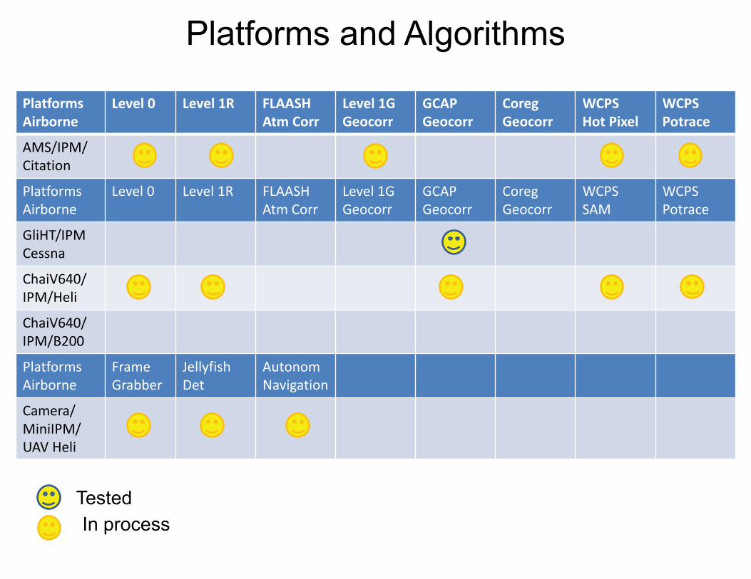
Platforms and Algorithms

Platforms Airborne

Level 0 Level 1R FLAASH Atm Corr

Level 1G Geocorr

GCAP Geocorr

Coreg Geocorr

WCPS Hot Pixel

WCPS Potrace

AMS/IPM/ Citation

Platforms Airborne

Level 0 Level 1R FLAASH Atm Corr

Level 1G Geocorr

GCAP Geocorr

Coreg Geocorr

WCPS SAM

WCPS Potrace

GliHT/IPM Cessna

ChaiV640/ IPM/Heli

ChaiV640/ IPM/B200

Platforms Airborne

Frame Grabber

Jellyfish Det

Autonom Navigation

Camera/ MiniIPM/ UAV Heli

Tested In process

Overview of Effort

• Year 1 Build hardware, begin writing software and arrange flights

• Year 2 Run simulated science scenarios (e.g. instrument calibrations)

• Year 2 Begin Flight tests • Year 2 Investigate software benchmarks • Year 3 More flight tests and benchmarks based on

results of year 2 • Year 3 Recommendations for future missions

5

Key Methods to Accelerate Onboard Computing for a Space Environment

• Intelligent onboard data reduction • Parallel processing, multicore processors • Use of FPGA as co-processor to accelerate portion

of algorithms

6

Example 1 of Intelligent Onboard Data Reduction: Autonomous

Modular Sensor Onboard Processing

7

DC Radiance

Reflectance

Temp. Hot Spots.

Scaled Visual Product.

FRP

Normalized Difference

Multi- Class Shapefile

Raw data

Intermediate

Derived Output “Real” Output

Existing Autonomous Modular Sensor (AMS) Pre-processing/Product Relationships

8

Burn Area Emergency Rehabilitation Imagery

BAER Bands:10 – 7 - 9Linear Stretched 2%

9

CCRS (Hot Pixels Algorithm) Provided OriginalWCPS Generated

10

Hot Pixels as Topojson on Github

http://geojson.io/#id=gist:cappelaere/770dc8388c021ca6091b&map=14/33.3553/-116.5015

Vectorized Hot Pixs to Topojson format ( 50% simplification)File Size: 6KB (2KB .tgz)

Topojson converted to C++ from javascript

Potrace integrated into WCPS

Displayed on MapBox TopoMap

Can be shared on Facebook/Twitter…All Open Source

11

Metrics

• Original AMS files size 3.1 Mbytes • Potrace – converts to raster to vector with the output being GeoJSON

– Geographic Javascript Object Notation (GeoJSON) file size is 31 kbytes • Topographic Javascript Object Notation (TopoJSON) converts GeoJSON to

TopoJSON format – file size is 6 kbytes (choose 50% simplification of vectors) – User selectable to about 90%

• Compress TopoJSON using ZIP – Compressed size is 2 kbyte

• Compression of 1000:1 • Download 2 kbyte GitHub then can visualize on built in map visualized (Mapbox)

– OpenStreetMap compatible – Viewable in browser – Shareable on Facebook and other social media – Github is used for versioning on maps and thus will store user annotation to

map

12

Example 2 for Intelligent Onboard Data Reduction: Running Coregistration with Chips

13

Global Land Survey Maps

• A collection of Landsat-type satellite images from USGS• Near complete global coverage• Orthorectified• Each image has cloud cover of less than 10%• Four versions: 1970, 1990, 2000, and 2005

• Ground truth for the registration programs was drawn from the GLS 2000 and can be updated when the GLS 2010 is completed

• http://landsat.usgs.gov/science_GLS.php14

Chip Registration

Overlapping chip from database

Chip extracted from EO1 scene

Area in EO1 scene where chip was extracted

Currently “chip database” created (in a brute-force fashion) by extracting successive 256x256 sub-images of all GLS scenes and storing them

according to path and row 15

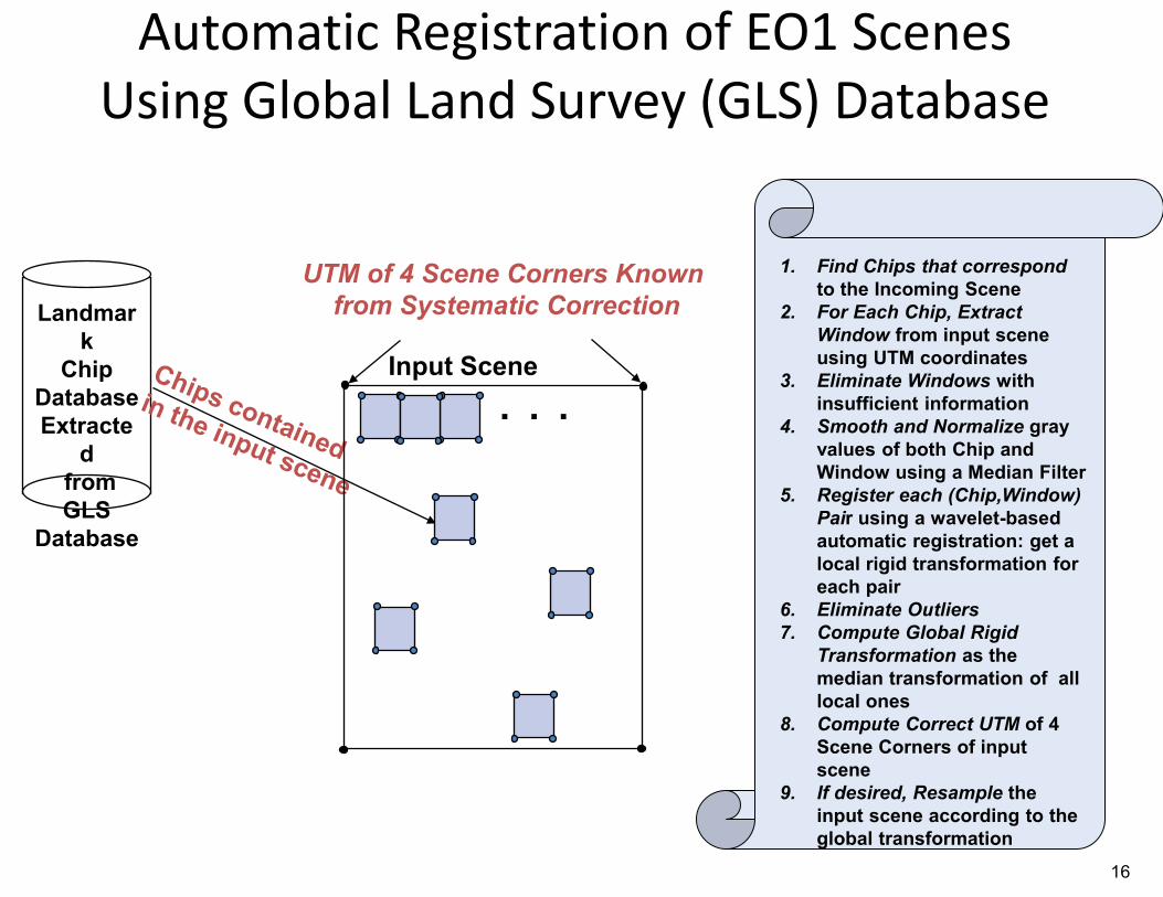
Automatic Registration of EO1 Scenes Using Global Land Survey (GLS) Database

Landmark

Chip DatabaseExtracte

dfrom GLS

Database

UTM of 4 Scene Corners Known from Systematic Correction

Input Scene

1. Find Chips that correspond to the Incoming Scene

2. For Each Chip, Extract Window from input scene using UTM coordinates

3. Eliminate Windows with insufficient information

4. Smooth and Normalize gray values of both Chip and Window using a Median Filter

5. Register each (Chip,Window) Pair using a wavelet-based automatic registration: get a local rigid transformation for each pair

6. Eliminate Outliers7. Compute Global Rigid

Transformation as the median transformation of all local ones

8. Compute Correct UTM of 4 Scene Corners of input scene

9. If desired, Resample theinput scene according to the global transformation

. . .

16

Scene 1 Before Automatic Registration Superimposed onto Goggle Earth

17

Scene 1 After Automatic Registration Superimposed onto Goggle Earth

18

Scene 2 Before Automatic Registration Superimposed onto Goggle Earth

19

Scene 2 After Automatic Registration Superimposed onto Goggle Earth

20

Conclusions and Future Work� Results visually acceptable

� Computations very fast and real-time

� RMS still too high (Translation errors between 0.4 and 2.5 pixels) because:

1. Chips and windows need to be pre-selected based on the information content (e.g., using an entropy measure)

� Registration would be more accurate because transformation would only be computed on pairs that have a significant amount of features

� Registration would be faster because less local registrations

� Chip database would be smaller to be stored onboard

2. Global transformation should be computed by taking the list of original corners coordinates of each window and their corresponding corrected coordinates, and treat them as a list of ground control points and their corresponding points => after outlier elimination, global transformation can be computed using a rigid, an affine or a polynomial transformation.

3. Masks for clouds and water should be included, so registration would not use cloud or water features that are often unreliable

• Onboard, computations can be performed on SpaceCube or hybrid processor 21

Representative IPM Data Processing Chain & Metrics

Building to Helicopter Experiment

Hyperspectral Image Processing Radiometric Correction (CHAI data)

*Atmospheric Correction (FLAASH) (EO1 Hyperion data)

Geometric Correction (GCAP) (GLiHT data)

*WCPS (vis_composite) (EO1 Hyperion data)

864 MHz TILEPro64 (1 core)

121.95 2477.74 183.42 72.39

864 MHz TILEPro64 (49 cores)

23.83 1744.13 4.59 21.63

1.0 GHz TILE-Gx36 (1 core)

57.22 897.71 28.51 19.93

1.0GHz TILE-Gx36 (36 cores)

9.21 588.71 1.41 8.72

2.2GHz Intel Core I7 2.09 58.29 0.169 2.26

Virtex 5 FPGA TBD TBD TBD TBD Image data: GLiHT 1004 x 1028 x 402 (829,818,048 bytes)Hyperion (EO1H1740732001151111K3) 256 x 6702 x 242 (830,404,608 bytes)Chai640 696 x 2103 x 283 (828,447,408 bytes)

Notes: Unit is in secondsTILEPro64 – No floating point supportTILEGx36 – Partial floating point support* Indicates time includes file I/O

23

FLAASH Parallelization Effort wall system user notes Parallelized?

Original Walltime

Parallel Speedup

Surf reflectance 32.7952 5.1398 27.6554Reflect::

RadtoRef YES 197.317 6.016642679

Cube smoothing 145.741 18.1373 127.6037mini_cube-

>Smooth; FFT

Cube reduction 112.363 13.9834 98.3796mini_cube->Condense

Cube load & distrib 89.0128 11.0775 77.9353

Cube gather & write 83.2988 10.3664 72.9324

Aerosol Retrieval 52.6236 6.54892 46.07468

Water col retrieval 34.7984 4.3306 30.4678

Spectral Polishing 33.5795 4.17891 29.40059

Sensor calibration 28.5097 3.54799 24.96171

Images and Masks 17.1781 2.13779 15.04031

Spectral Resampling 8.72743 1.08611 7.64132Smile_Resampler::Cube_Copy YES 241.669 27.69074057

Cloud Masking 5.93287 0.738336 5.194534

Sensor slit function 0.764612 0.0951547 0.6694573

Modtran Tables 0.416416 0.0518223 0.3645937

un-categorized 0.0397966 0.00495262 0.03484398

Flaash setup 0.000163794 2.04E-05 1.43E-04

total time 645.7813884 81.425006 564.3563824 1.641422344

total time (h:m:s) 0:10:46 0:01:21 0:09:24

Original Wall time: 1060

0:17:4024

5%

23%

17%

14%

13%

8%

5%

5%

4%

3% 1%

1% 0%

0% 0%

0%

Time spent in FLAASH components

Surf reflectance

Cube smoothing

Cube reduction

Cube load & distrib

Cube gather & write

Aerosol Retrieval

Water col retrieval

Spectral Polishing

Sensor calibration

Images and Masks

Spectral Resampling

Cloud Masking

Sensor slit function

Modtran Tables

un-categorized

Flaash setup

25

Conclusion� Examining a variety of methods to speed up onboard

processing chain to meet needs of low latency users

� Dovetailing efforts and metrics with High Performance Space Computing (HPSC) effort sponsored by NASA Office Chief Technologist

� IPM data processing effort applied to multiple future mission needs

26