proton transport mechanisms of phosphoric acid and related
TRANSCRIPT

Proton Transport Mechanisms ofPhosphoric Acid and RelatedPhosphorus Oxoacid Systems:A First Principles Molecular
Dynamics Study
Von der Fakultat Chemie der Universitat Stuttgartzur Erlangung der Wurde eines
Doktors der Naturwissenschaften (Dr. rer. nat.)genehmigte Abhandlung
Vorgelegt von
Linas Vilciauskasaus Joniskis, Litauen
Hauptberichter: Prof. Dr. Joachim MaierMitberichter: Jun. Prof. Dr. Johannes KastnerPrufungsvorsitzender: Prof. Dr. Emil Roduner
Tag der mundlichen Prufung: 06.02.2012
Max-Planck-Institut fur FestkorperforschungUniversitat Stuttgart
2012

ii

To my parents, all of my mentors and the memory of a fellowcountryman C. J. D. Theodor von Grotthuß – pioneer of physical
chemistry
Mano tevams, visiems mokytojams ir krastiecio, fizikines chemijospradininko – C. J. D. Theodor’o von Grotthuss’o atminimui

ii

Das ewig Unbegreifliche an der Welt ist ihre Begreiflichkeit.
Albert Einstein (1879-1955)‘Physik und Realitat’
Journal of the Franklin Institute 1936, 122, 315.

iv

Erklarung
Die vorliegende Doktorarbeit wurde vom Autor selbst in der Abteilungvon Prof. Maier und in der Max-Planck-Forschergruppe Theorie vonHalbleiternanostrukturen am Max-Planck-Institut fur Festkorperfor-schung, im Zeitraum von Januar 2008 bis November 2011 angefertigt.Der Inhalt ist die eigene Arbeit des Autors, Ausnahmen sind gekenn-zeichnet, und wurde noch nicht zur Erlangung einer Qualifizierungoder eines Titels an einer akademischen Institution eingereicht.
Stuttgart, den 16. Dezember 2011 Linas Vilciauskas
Declaration
The work described in this thesis was carried out by the author in theDepartment of Prof. Maier and in the Max Planck Research GroupTheory of Semiconductor Nanostructures at the Max Planck Institutefor Solid State Research from January 2008 to November 2011. Thecontents are the original work of the author except where indicatedotherwise and have not been previously submitted for any other de-gree or qualification at any academic institution.
Stuttgart, 16 December 2011 Linas Vilciauskas

vi

Acknowledgements
I would like express the utmost gratitude to my supervisor Dr. Klaus-Dieter Kreuer. First of all, for offering this topic for my PhD thesisand introducing me to the field of proton conductors. Secondly, forproviding me the excellent funding opportunities and, certainly, forthe infinite supply of ideas during the execution of this project. It wasan enormous pleasure to be guided through this field by one of theleading experts. I am sure that our lengthy discussions during lunch,coffee and ‘post-coffee’ breaks on subjects ranging from protons inphosphoric acid to politics, religion or philosophy had a strong impacton my scientific and personal development.
The support, freedom and trust provided by the head of the depart-ment Prof. Dr. Joachim Maier for this project must be greatly ac-knowledged. In addition, I would also like to thank him and the othermembers of the examination committee: Prof. Dr. E. Roduner andJProf. Dr. J. Kastner for agreeing to take the responsibility of thefinal doctoral examination.
I sincerely appreciate the help and support provided by my co-supervisorDr. Gabriel Bester, without whom this project, most probably, wouldhave not even been born. In spite of likely being the most friendly andopen person I have ever met, he also eagerly agreed to collaborate onthis work and provided invaluable guidance and immense computerresources throughout. I certainly learned a lot from him and trulybenefited from our discussions on the computational science, densityfunctional theory and many other aspects of physics and ‘daily’ life.
I would like to express my greatest thanks to one of my ‘key mentors’ –Prof. Mark E. Tuckerman (New York University) for keenly agreeingto collaborate on this project right from the first minute and providingan invaluable help and advice on basically every single aspect of thiswork. In addition to being one of the world’s leading experts on abinitio molecular dynamics and proton transport, Mark proved to bean extremely friendly and approachable person. His comments andideas were key for this project in reaching its final shape and success.
My warm thanks go to Prof. Stephen J. Paddison (University of Ten-nessee, Knoxville), a ‘long-time’ collaborator of mine, for his fruitfulcontribution to this project, right from the ‘start line’. His commentsand critique were always a valuable source of information for improv-ing many aspects of this work.
I would kindly like to thank Dr. Bernhard Frick (Institut Laue-Langevin, Grenoble) for introducing me to the fascinating world ofneutrons. I really enjoyed the fruitful work and discussions withBernhard on quasi-elastic neutron scattering and its use for studyingproton dynamics and transport during my several visits to Grenoble.
I am thankful to Dr. Carla C. de Araujo for the nice time, fruitfulcollaboration and discussions as well as providing important experi-mental input for the work on pure phosphinic acid.
I am also indebted to all the people at the FKF-EDV group (A. Schuh-macher, U. Traub, A. Burkhardt, K. Roßmann) for the very nice work-ing environment and help with technical difficulties. RechenzentrumGarching der Max-Planck-Gesellschaft is also greatly acknowledgedfor their support and opportunity to use the VIP machine.
I appreciate all of my friends and colleagues who provided a nice atmo-sphere in and outside of the Max Planck Institute during the time ofmy PhD studies. My thanks for the nice time spent together go to theLithuanian, Anglo-Saxon, Russian communities and many other indi-viduals: S. C. White, J. M. Law, P. M. R. Brydon, V. Alexandrov, D.Gryaznov, Y. Mastrikov, I. Pentin, I. Pentegov, D. Zagorac, J. Bauer,C. Schon, L. Krisciunaite, M. Lipschis, E. Stasaitis, J. Kaiser andmany others. I would also like to thank my good friends and colleaguessince my time in Vilnius, with whom I kept a lot of contacts and hadsome wonderful time while not doing my research: A. Bambalas (Vil-nius), L. Zakrys (Glasgow), V. Lapiene (Dortmund), G. Gasiunas(Vilnius), V. Navickas (Tubingen/Ludwigshafen), K. Klemkaite (Vil-nius), G. Muizis (Vilnius) and others.
Most importantly, I’d like to thank my parents and my sister Jurgitafor their continual support and belief in my feat and success.
I would also like to acknowledge those thousands of individuals whohave contributed to all the open source projects, including the main‘workhorses’ CPMD, CP2K and VMD as well as LATEX, used for typesettingthis thesis.

Abstract
Fundamental understanding of proton transport in hydrogen bonded systems on
the molecular level remains a key problem in many areas of science ranging from
electrochemical energy conversion to biological systems. Despite the enormous
advances in the research of these processes, the ostensibly simplest case, proton
transport in homogeneous bulk media at thermodynamic equilibrium, proved to
be one of the most challenging and elusive. The large number of nontrivially
coupled reaction coordinates involved in the formation and transport of protonic
defects render the task of extracting the molecular level mechanisms a formidable
one. It is only through enormous theoretical and experimental efforts that clear
mechanistic pictures of the transport of excess protonic charge defects (H3O+
and OH−) in water have emerged. However, water has negligible intrinsic pro-
ton conductivity. By contrast, the class of compounds known as phosphorus
oxoacids have some of the highest reported proton conductivities. In this work,
the molecular level proton transport mechanisms in this family of proton con-
ductors (H3PO4, H3PO3 and H3PO2) and some closely related systems (H3PO4
- H2O mixtures) are investigated with the help of ab initio molecular dynamics
simulations. In fact, neat liquid phosphoric acid has the highest intrinsic proton
conductivity of any known substance. Apart from playing a central role in the
structure and function of biological systems (e.g. ATP, DNA, lipid membranes),
systems containing phosphates/phosphonates (e.g. PBI/H3PO4) are attracting
an increasing interest as high-temperature electrolytes for emerging fuel cell ap-
plications.
For the first time, the microscopic mechanisms of the proton transport phe-
nomenon in these systems are revealed with an appropriate spatial and temporal
resolution. The results show that strong, mutually polarizable hydrogen bonds
ix

give rise to coupled proton motion and a pronounced protic dielectric response
of the medium. This allows for the formation of extended, polarized hydrogen
bonded (Grotthuss) chains, never truly observed in bulk hydrogen bonded sys-
tems. The results show that, in phosphoric acid, the central system of this study,
such chains containing up to five consecutive hydrogen bonds can form. It is
the interplay between these chains and a frustrated (there are more proton donor
than acceptor sites) hydrogen bond network, which is found to lead to extremely
high proton conductivity in phosphoric acid. This strongly contrasts to water,
wherein the anomalously high rate of excess charge transport occurs not through
extended chains but rather through local hydrogen bond rearrangements that drive
individual proton transfer reactions. The mechanism proposed in this work, sug-
gests that strong hydrogen bonding does not necessarily lead to protonic ordering
and slow dynamics of the system, demonstrating that weak solvent coupling and
sufficient degree of configurational disorder can lead to fast proton transport.
Although, phosphonic and phosphinic acids possess even stronger hydrogen
bonds, the stronger dipolar and dynamic backgrounds tend to oppose the for-
mation of extended Grotthuss chains. Moreover, these systems do not have the
same intrinsically frustrated hydrogen bond network (there are more proton accep-
tor than donor sites), thus hindering the solvent reorganization (depolarization).
Nevertheless, the results show that the weak hydrogen bonded configurations,
although not an intrinsic property of the hydrogen bond network, are still form-
ing in a dynamical sense due to liquid disorder. The latter, together with the
formation of polarized chains explain the high charge carrier concentrations and
conductivities reported in these materials, especially in H3PO3, where they are
only slightly lower than in the case of H3PO4.
Apparently, proton transport in phosphoric acid is extremely susceptible to
nearly all types of chemical perturbations. Apart from the severe conductiv-
ity reduction caused by the addition of bases, even the addition of acids leads to
some decrease in conductivity. The only dopant that increases the conductivity of
H3PO4 is water which, together with some condensation products (e.g. H4P2O7,
H5P3O10) is already present even in a nominally dry acid under the conditions
of thermodynamic equilibrium. In fact, the severe increase in the conductivity
of phosphoric acid upon dilution cannot be explained by simple hydrodynamic
x

diffusion of hydronium ion, indicating that proton structural diffusion plays a
major role in these systems as well. The results show that very similar molecular
mechanisms are at play in phosphoric acid – water system as in neat oxoacid
systems. The properties of hydrogen bonds even in 1:1 H3PO4 − H2O mixture
are virtually identical to those of pure H3PO4, generally, showing no resemblance
to liquid H2O. It is due to the strong and polarizable acid-water hydrogen bonds,
that some degree of cooperativity can still be observed in the proton transport
mechanism, although the solvent coupling in this case is much stronger due to
the significantly different dielectric nature of the water phase. In addition to
some vehicular contribution to proton conductivity, water also has some plasti-
cizing effect, increasing the configurational disorder in the hydrogen bond net-
work, therefore resulting in significantly higher conductivities observed in these
systems.
xi

xii
Zusammenfassung
Das grundlegende Verstandnis der Protonen-Transport-Mechanismen in Wasser-
stoffbrucken gebundenen Medien auf molekularer Ebene bleibt eine der zentralen
Fragen in vielen Bereichen der Wissenschaft, angefangen von elektrochemischer
Energieumwandlung bis hin zu Prozessen in biologischen Systemen. Trotz der
starken Fortschritte in der Erforschung dieser Prozesse, erwies sich der vermeint-
lich einfachste Fall – Protonentransport in homogenen Bulk-Medien im thermo-
dynamischen Gleichgewicht – als einer der herausforderndsten und am schwersten
fassbaren. Die große Zahl der nichttrivial gekoppelten Reaktionskoordinaten, die
an der Bildung und der Wanderung der Protonen-Defekte beteiligt sind, machen
das Herausarbeiten der molekularen Details dieser Mechanismen zu einer sehr
schwierigen Aufgabe. Nur durch enorme theoretische und experimentelle Anstren-
gungen war es moglich, eine klare mechanistische Darstellung des Transports von
protononischen Defekten (H3O+ und OH− Ionen) in Wasser zu entwickeln. Wasser
hat jedoch eine geringe intrinsische Protonenleitfahigkeit. Im Gegensatz dazu hat
eine Klasse von Verbindungen, die unter dem Namen Phosphor-Oxosauren be-
kannt ist, einige der hochsten bekannten Protonenleitfahigkeiten. In dieser Arbeit
werden die Protonen-Transport -Mechanismen dieser Familie von Protonenleitern
(H3PO4, H3PO3 and H3PO2) und einigen eng verwandten Systemen (H3PO4 -
H2O Mischungen) mit Hilfe von ab initio Molekulardynamik-Simulationen auf
molekularer Ebene untersucht. Reine flussige Phosphorsaure hat die hochste in-
trinsische Protonenleitfahigkeit aller bekannten Substanzen. Abgesehen davon,
dass Phosphate eine zentrale Rolle in der Struktur und Funktion von biologi-
schen Systemen (z. B. ATP, DNA, Lipid-Membranen) spielen, sind Systeme, die
Phosphsate/Phosphonate enthalten (z. B. PBI/H3PO4), von zunehmendem In-
teresse als Hochtemperatur-Elektrolyte in Brennstoffzellen.
xiii

Die vorliegende Arbeit gibt ertsmalig Einblicke in die mikroskopischen Details
der Protonen-Ttransport-Mechanismen in diesen Systemen mit einer geeigneten
raumlichen und zeitlichen Auflosung. Die Ergebnisse zeigen, dass starke, pola-
risierbare Wasserstoffbrucken an einer gekoppelten Protonenbewegung und aus-
gepragten protonischen dielektrischen Antwort des Mediums beteiligt sind. Dies
erlaubt die Bildung ausgedehnter, polarisierter Wasserstoffbrucken gebundener
(Grotthuss-) Ketten, die zuvor noch nie in einem Bulk-System beobachtet wur-
den. Die Ergebnisse zeigen, dass sich in Phosphorsaure, dem zentralen System der
vorliegenden Arbeit, solche Ketten von bis zu funf aufeinander folgenden Was-
serstoffbrucken bilden konnen. Es ist das Zusammenspiel dieser Ketten mit ei-
nem frustrierten Wasserstoffbrucken-Netzwerk (es gibt mehr Protonen-Akzeptor-
als Donorstellen), das, wie herausgefunden wurde, zu der bekannten extrem ho-
hen Protonenleitfahigkeit in Phosphorsaure fuhrt. Der beobachtete Mechsnismus
unterscheidet sich wesentlich von dem wassriger Medien, in denen die hohe Be-
weglichkeit protonischer Ladungstrager nicht durch die Dynamik langer Ketten,
sondern durch lokale Umlagerungen der Wasserstoffbrucken, die die einzelnen
Protonen-Ubertragungs-Reaktionen auslosen, hervorgerufen wird. Der in dieser
Arbeit vorgeschlagene Mechanismus legt nahe, dass starke Wasserstoffbrucken-
bindungen nicht gezwungenermaßen zu Protonen-Ordnung und langsamer Dyna-
mik des Systems fuhren mussen, sondern zeigt, dass schwache Losungsmitteleffek-
te und ein ausreichender Grad der Konfigurations-Fehlordnungung zu schnellem
Protonen-Transport fuhren konnen.
Obwohl, die Phosphon- und Phosphinsauren noch starkere Wasserstoffbin-
dungen aufweisen, ist die Bildung von Grotthuss-Ketten durch den starker di-
polaren Charakter des Solvents und wegen der ausgepragteren lokalen Dynamik
(die Wasserstoffbruckendichte ist niedriger als in Phosphorsaure) auf kurzere Ket-
tenlangen begrenzt. Hinzu kommt, dass die Wasserstoffbrucken-Netzwerke dieser
Systeme lediglich dynamisch frustriert sind, wodurch auch die Rate der Depolari-
zationsreaktionen reduziert ist. Die thermisch aktivierte Konzetration nicht uber
Wasserstoffbrucken gebundener OH Gruppen ist jedoch noch so hoch, dass po-
larisierte, wenn auch kurze, Grotthuss-Ketten, hinreichend schnell depolarisiert
werden konnen. Dies erklart insbesondere die Leitfahigkeit von H3PO3, die nur
geringfugig niedriger als die von H3PO4 ist.
xiv

Der Protonentransport in Phosphorsaure ist offensichtlich extrem anfallig
fur chemische Storungen fast aller Arten. Abgesehen von der starken Leitfahig-
keitsminderung durch die Zugabe von Basen, fuhrt aber auch die Zugabe von
Sauren zu einer gewissen Erniedrigung der Leitfahigkeit. Der einzige Zusatz,
der die Leitfahigkeit von H3PO4 erhoht ist Wasser, das zusammen mit einigen
Kondensationsprodukten (z. B. H4P2O7, H5P3O10) bereits in nominell trockener
Saure im thermodynamischen Gleichgewicht vorliegt. Tatsachlich kann die star-
ke Erhohung der Leitfahigkeit nach Verdunnung von Phosphorsaure nicht durch
einfache hydrodynamische Diffusion von Hydronium-Ionen erklart werden, was
darauf hindeutet, dass auch die Protonen-Strukturdiffusion eine wichtige Rol-
le in diesen Systemen spielt. Die vorliegenden Ergebnisse zeigen, dass sich der
Protononenleitmechanismus durch Zugabe von Wasser zunachst kaum andert.
Die Eigenschaften von Wasserstoffbruckenbindung in einer 1:1 H3PO4-H2O Mi-
schung, sind praktisch identisch mit denen der reinen H3PO4 und zeigen keine
Ahnlichkeit mit denen in flussigem H2O. Es sind die starken und polarisierbaren
Saure-Wasser-Wasserstoffbruckenbindungen, die in diesen Systemen noch einen
gewisser Grad an Kooperativiat im Mechanismus des Protonen-Transports zulas-
sen. Neben einem gewissen Vehikel-Beitrag zur Protonenleitfahigkeit hat Wasser
auch eine weichmachende Wirkung, die die Konfigurations-Fehlordnung im Was-
serstoffbrucken-Netzwerk erhoht und so zu den deutlich hoheren Leitfahigkeiten
dieser Systeme beitragt.
xv

xvi

Contents
Abstract ix
Zusammenfassung xiii
List of Figures xxi
List of Tables xxvii
1 Introduction 1
1.1 Proton Transport . . . . . . . . . . . . . . . . . . . . . . . . . . . 1
1.1.1 Proton Transport in Water . . . . . . . . . . . . . . . . . . 5
1.1.2 Phosphorus Oxoacids . . . . . . . . . . . . . . . . . . . . . 9
1.1.3 PEMFC Materials based on Phosphorus Oxoacids . . . . . 16
1.2 Ab Initio Molecular Dynamics . . . . . . . . . . . . . . . . . . . . 18
1.2.1 Density Functional Theory . . . . . . . . . . . . . . . . . . 20
1.2.2 Born-Oppenheimer Molecular Dynamics . . . . . . . . . . 23
1.2.3 Car-Parrinello Molecular Dynamics . . . . . . . . . . . . . 24
1.2.4 Evaluation of forces in AIMD . . . . . . . . . . . . . . . . 26
1.2.5 Basis Sets . . . . . . . . . . . . . . . . . . . . . . . . . . . 27
1.2.6 Pseudopotentials . . . . . . . . . . . . . . . . . . . . . . . 31
1.2.7 Beyond Microcanonics: Thermostatting . . . . . . . . . . . 33
1.2.8 Equilibrium Time Correlation Functions . . . . . . . . . . 34
2 Aims of the project 37
3 Computational methods and setup 39
xvii

CONTENTS
4 Phosphoric acid 43
4.1 Structural Properties . . . . . . . . . . . . . . . . . . . . . . . . . 43
4.2 Dynamical Properties . . . . . . . . . . . . . . . . . . . . . . . . . 45
4.3 Rotational Dynamics . . . . . . . . . . . . . . . . . . . . . . . . . 48
4.4 Proton Transfer Kinetics . . . . . . . . . . . . . . . . . . . . . . . 50
4.5 Proton Transfer Energetics . . . . . . . . . . . . . . . . . . . . . . 52
4.6 The Structure and Energetics of Charged Species . . . . . . . . . 54
4.7 On the Degree of Protonation . . . . . . . . . . . . . . . . . . . . 56
4.8 Interprotonic Coupling . . . . . . . . . . . . . . . . . . . . . . . . 58
4.9 Formation of Grotthuss Chains . . . . . . . . . . . . . . . . . . . 62
4.10 On the Proton Transport Mechanism . . . . . . . . . . . . . . . . 65
5 Phosphonic and phosphinic acids 69
5.1 Structural Properties . . . . . . . . . . . . . . . . . . . . . . . . . 69
5.2 Dynamical Properties . . . . . . . . . . . . . . . . . . . . . . . . . 73
5.3 Vibrational spectra . . . . . . . . . . . . . . . . . . . . . . . . . . 79
5.4 Proton Transfer Kinetics . . . . . . . . . . . . . . . . . . . . . . . 81
5.5 Proton Transfer Energetics . . . . . . . . . . . . . . . . . . . . . . 83
5.6 The Structure and Energetics of Charged Species . . . . . . . . . 84
5.7 On the Degree of Protonation . . . . . . . . . . . . . . . . . . . . 87
5.8 Interprotonic Coupling . . . . . . . . . . . . . . . . . . . . . . . . 89
5.9 On the Formation of Grotthuss Chains and Proton Conduction
Mechanisms . . . . . . . . . . . . . . . . . . . . . . . . . . . . . . 91
6 Phosphoric acid and water mixtures 97
6.1 Structural Properties . . . . . . . . . . . . . . . . . . . . . . . . . 98
6.2 Dynamical Properties . . . . . . . . . . . . . . . . . . . . . . . . . 102
6.3 Proton Transfer Energetics and the State of Charged Species . . . 104
6.4 Interprotonic Coupling . . . . . . . . . . . . . . . . . . . . . . . . 107
6.5 On the Formation of Grotthuss Chains and Proton Transport Mech-
anism . . . . . . . . . . . . . . . . . . . . . . . . . . . . . . . . . 109
7 Conclusions 115
xviii

CONTENTS
References 119
Lebenslauf 127
xix

CONTENTS
xx

List of Figures
1.1 Temperature dependent conductivities of the various classes of pro-
ton conducting materials. . . . . . . . . . . . . . . . . . . . . . . . 4
1.2 Excess proton structural diffusion in water. The hydrogen bonds
around the excess charge are contracted, favoring the PT and the
hydrogen-bond breaking and forming processes occur in the more
loosely bound outer hydration shells. The proton potentials show
the adiabatic transfer of the central proton.2,3,6 . . . . . . . . . . 7
1.3 Structure of phosphoric (left), phosphonic (middle) and phosphinic
(right) acid molecules. Different coloring correspond to different
atoms: phosphorus (purple), oxygen (red) and hydrogen (white). . 10
1.4 Mechanism of proton conduction in phosphoric acid based on PFG-
NMR and conductivity data.68. . . . . . . . . . . . . . . . . . . . 12
1.5 Temperature dependence of 1H and 31P diffusion coefficients.68. . 13
1.6 H/D isotope effect for the diffusion of 1H and 2H(D) in mixtures
of H3PO4 and D3PO4.80 . . . . . . . . . . . . . . . . . . . . . . . 14
3.1 Variation of the total energy (conserved quantity), electronic ki-
netic energy (Car-Parrinello) and temperature (classical kinetic en-
ergy of the nuclei) during the CPMD simulation. . . . . . . . . . . . 41
3.2 Variation of the total energy (conserved quantity) and temperature
(clasical energy of the nuclei) during the CP2K simulation. . . . . . 42
4.1 A snapshot of a typical configuration from an equilibrated simula-
tion box containing 54 H3PO4 molecules. . . . . . . . . . . . . . . 44
xxi

LIST OF FIGURES
4.2 Radial pair distribution functions of liquid phosphoric acid. The
results of two simulations are compared to the neutron scattering
study.156 The gHX and gXX are defined in the same way as in the
experimental work: (gHX(r) = 0.823gHO(r) + 0.182gHP(r); gXX(r)
= 0.673gOO(r) + 0.298gOP(r) + 0.033gPP(r)). . . . . . . . . . . . . 46
4.3 Average mean square displacements and corresponding diffusion
constants as obtained from the Einstein relation for hydrogen and
phosphorus atoms in H3PO4 at 383 K. . . . . . . . . . . . . . . . 48
4.4 The average angular displacement of the P–O bond with respect
to time and the corresponding rotational diffusion constant. . . . 50
4.5 Orientational correlation functions Cn for the uP−O bond. n =
1,2,3 are shown. . . . . . . . . . . . . . . . . . . . . . . . . . . . . 51
4.6 Proton transfer population correlation functions (including and ex-
cluding proton rattling) and their triexponential fits. . . . . . . . 53
4.7 P(ROO, δ) probability distribution . . . . . . . . . . . . . . . . . . 54
4.8 Free energy profile A(δ) along the proton transfer coordinate δ. . 54
4.9 RDFs gOO and running coordination numbers (nOO) of oxygen
atoms for phosphoric acid in its various states of protonation. . . 56
4.10 Free energy profiles A(δ) along the proton transfer coordinate δ for
H3PO4, H4PO+4 and H2PO−4 . . . . . . . . . . . . . . . . . . . . . . 57
4.11 The probability distribution of oxygen protonation states defined
as the sum of individual bond-orders due to surrounding protons
(∑ni). . . . . . . . . . . . . . . . . . . . . . . . . . . . . . . . . . 58
4.12 Absolute magnitude of a purely electrostatic force F (t) acting on
a transferring proton (δ → 0; time = 0 ps) due to all other protons
in the system.171 . . . . . . . . . . . . . . . . . . . . . . . . . . . 60
4.13 gHH(H3PO4) radial distribution function resolved in r and δ, con-
taining information about the spatial distribution of protons with
respect to δ (δeq is the equilibrium value in the simulation).171 . . 60
4.14 gPP RDF resolved in r and δ. . . . . . . . . . . . . . . . . . . . . 61
4.15 The running coordination numbers nOO(r,δ) resolved in δ and r
for donating and accepting oxygen atoms. . . . . . . . . . . . . . 61
xxii

LIST OF FIGURES
4.16 Proton coupling correlation function Cpc(n) as a function of con-
nectivity n. Specific values include n = 0, (single H-bond), 1 (ad-
jacent H-bonds), and 6 (longest non-cyclic path in the H-bond
network). Only the H-bonds with δ ≤ 0.1 A (only ∼ 1.5% of the
total number) are considered as undergoing PT. The time incre-
ment τres sets the finite relay time for the system to respond to
correlated PTs.171 . . . . . . . . . . . . . . . . . . . . . . . . . . . 64
4.17 Snapshots of the elementary steps of the proton structural diffu-
sion mechanism in H3PO4. This sample event shows five molecules
extracted from the simulation box, which participate in the cor-
related PTs over four neighboring H-bonds and in the formation
of a Grotthuss chain. The schemes below the molecular structures
show the ions and the interchain dipoles, with the remaining sol-
vent molecules represented by a generalized coordinate ~S. The
arrows denote the PTs and molecular reorientations for the im-
portant steps in the mechanism: (a) and (b) correlated PTs and
formation of a Grotthuss chain; (c) and (d) reorientation of the
solvent H3PO4 molecule induced by the formation and breaking of
the ‘frustrated’ H-bond; (e) and (f) formation and breaking of the
second ‘frustrated’ H-bond.171 . . . . . . . . . . . . . . . . . . . . 68
5.1 Snapshots representing the typical configurations from an equi-
librated simulation boxes containing (a) 54 H3PO3 and (b) 54
H3PO2 molecules. . . . . . . . . . . . . . . . . . . . . . . . . . . . 70
5.2 The full simulated radial pair distribution function gXX (where X
= P, O and H) and gXX from the neutron scattering study.95 . . . 71
5.3 Radial pair distribution functions for the liquid H3PO4, H3PO3
and H3PO2. (top) gHOHOonly for the acidic protons (excluding
the hydrogens covalently bonded to phosphorus). (middle) gOHO
for the acidic protons and oxygen atoms, the first peak comes form
the covalent O–H bond and the second due to the H-bonding (H· · ·O). (bottom) gXX, where X = P or O, shows the different heavy
atom pair contributions. . . . . . . . . . . . . . . . . . . . . . . . 72
xxiii

LIST OF FIGURES
5.4 H-bond geometries for H3PO4 (black), H3PO3 (red) and H3PO2
(green): probability distributions for (left) RO...O distances, and
αO−H...O angles. . . . . . . . . . . . . . . . . . . . . . . . . . . . . 73
5.5 Proton and molecular diffusion coefficients determined by the PFG-
NMR with respect to temperature.66 . . . . . . . . . . . . . . . . 77
5.6 Conductivities and the respective contributions due to structural
diffusion in H3PO4, H3PO3 and H3PO2.66 . . . . . . . . . . . . . . 78
5.7 The average angular displacement of the P–O bond with respect
to time and the corresponding rotational diffusion constants for
H3PO4, H3PO3 and H3PO2 at 383 K. . . . . . . . . . . . . . . . . 80
5.8 Average mean square displacements and corresponding diffusion
constants as obtained from the Einstein relation for hydrogen and
phosphorus atoms in H3PO4 at 383 K. . . . . . . . . . . . . . . . 81
5.9 Comparison of the vibrational power spectra for H3PO4, H3PO3
and H3PO2. . . . . . . . . . . . . . . . . . . . . . . . . . . . . . . 82
5.10 Proton transfer population correlation functions (including and ex-
cluding proton rattling) and their triexponential fits for H3PO3. . 83
5.11 Proton transfer population correlation functions (including and ex-
cluding proton rattling) and their triexponential fits for H3PO2. . 84
5.12 Free energy profiles A(δ) along the proton transfer coordinate δ for
H3PO4, H3PO3 and H3PO2. . . . . . . . . . . . . . . . . . . . . . 85
5.13 gOO and running coordination numbers (nOO) of oxygen atoms for
H3PO3 in its various states of protonation. . . . . . . . . . . . . . 87
5.14 gOO and running coordination numbers (nOO) of oxygen atoms for
H3PO2 in its various states of protonation. . . . . . . . . . . . . . 88
5.15 Free energy profiles A(δ) along the proton transfer coordinate δ for
H3PO3, H4PO+3 and H2PO−3 . . . . . . . . . . . . . . . . . . . . . . 89
5.16 Free energy profiles A(δ) along the proton transfer coordinate δ for
H3PO2, H4PO+2 and H2PO−2 . . . . . . . . . . . . . . . . . . . . . . 90
5.17 The probability distribution of various oxygen protonation states
defined as the sum of individual bond-orders due to surrounding
protons (∑ni). . . . . . . . . . . . . . . . . . . . . . . . . . . . . 91
xxiv

LIST OF FIGURES
5.18 gHH(r, δ; H3PO3) radial distribution function resolved in r and δ,
containing information about the spatial distribution of protons
with respect to δ (δeq is the equilibrium value in the simulation). . 92
5.19 gHH(r, δ; H3PO2) radial distribution function resolved in r and δ,
containing information about the spatial distribution of protons
with respect to δ (δeq is the equilibrium value in the simulation). . 93
5.20 Proton coupling correlation function Cpc(n) as a function of con-
nectivity n. Only the H-bonds with δ ≤ 0.1 A (∼ 2.0% of the
total number for H3PO3 and ∼ 3.5% for H3PO2) are considered as
undergoing PT. The time increment τres sets the finite relay time
for the system to respond to correlated PTs (τres = 50 fs). . . . . 94
5.21 Snapshots of the elementary the proton structural diffusion steps
in H3PO2. The schemes bellow the molecular structures show the
ions and interchain dipole orientations, with the solvent being rep-
resented by a generalized coordinate ~S. The charged ion pair is
indicated with (+) and (-), the partial charges on the oxygen atoms
are marked by +δ and −δ. The arrows denote the proton hops and
molecular reorientations. . . . . . . . . . . . . . . . . . . . . . . . 96
6.1 A snapshot of a typical configuration from an equilibrated simula-
tion box containing 36 H3PO4 and 36 H2O molecules. . . . . . . . 98
6.2 The total simulated radial pair distribution function gXX (black)
(where X = P, O and H) and gXX (red) from the neutron scattering
study of Kameda et al.189 . . . . . . . . . . . . . . . . . . . . . . 99
6.3 Radial pair distribution functions of the H3PO4 water solutions.
The structure of neat H3PO4 and H2O are given for comparison.
(top) gHH for System II, H3PO4 and H2O. (middle) gOH for for
System I, System II, H3PO4 and H2O; the first peak comes form the
covalent O–H bond and the second due to the H-bonding (H. . . O).
(bottom) gXX, where X = P or O, shows the different contributions
from heavy atom pairs to the total RDF. . . . . . . . . . . . . . . 101
xxv

LIST OF FIGURES
6.4 Average mean square displacements and corresponding diffusion
constants as obtained from the Einstein relation for hydrogen, oxy-
gen and phosphorus atoms in System II at 383 K. . . . . . . . . . 104
6.5 Vibrational spectrum for System II (H3PO4 + H2O (1:1)) (blue)
and H3PO4 (black). . . . . . . . . . . . . . . . . . . . . . . . . . . 105
6.6 Free energy profiles ∆A(δ) along the proton transfer coordinate δ
for PT between phosphoric acid and water for System I. . . . . . 107
6.7 Free energy profiles ∆A(δ) along the proton transfer coordinate δ
for all protons and different proton donor/acceptor pairs in System
II. . . . . . . . . . . . . . . . . . . . . . . . . . . . . . . . . . . . 108
6.8 gHH(SystemII) radial distribution function resolved in r and δ,
containing information about the spatial distribution of protons
with respect to δ (δeq is the equilibrium value in the simulation). . 109
6.9 Proton coupling correlation function Cpc(n) as a function of con-
nectivity n for pure H3PO4 and System II. δcut ≤ 0.1 A and τres =
0 and 50 fs. . . . . . . . . . . . . . . . . . . . . . . . . . . . . . . 111
6.10 Snapshots of the elementary proton structural diffusion steps in
System II. The charged ion pair is indicated with (+) and (-). The
arrows denote the proton hops and molecular reorientations. . . . 113
xxvi

List of Tables
5.1 Calculated and experimental diffusion coefficients at 383 K for
phosphonic and phosphinic acids. . . . . . . . . . . . . . . . . . . 79
5.2 Calculated fractions of molecules with uncompensated protonic
charge (having excess or deficient protons) for H3PO4, H3PO3 and
H3PO2 systems and different proton assignment criteria δcut−off . . 86
6.1 Calculated fractions of water and phosphoric acid molecules in
their different states of protonation in System II, with different
proton assignment criterion δcut−off . . . . . . . . . . . . . . . . . . 106
xxvii

LIST OF TABLES
xxviii

1
Introduction
1.1 Proton Transport
The molecular understanding of proton transport is one of the long-standing
problems in many areas of science ranging from electrochemical energy conver-
sion to biological systems.1–5 Despite the vast advances in the understanding of
these processes, the apparently simplest case of proton transport in bulk media
under the conditions of thermodynamic equilibrium, appears to be the most chal-
lenging.3,6 The complication arises due the high number of solvent coordinates
and a nontrivial coupling between the coordinates of the solvent and those of the
protonic defects. In large part thanks to ab initio molecular dynamics (AIMD)
simulations, water became the first and remains the only extended H-bonded sys-
tem for which a molecular picture of protonic defect transport has been envisioned
in great detail.7–25
A big part of the motivation for this work stems not just from the fundamen-
tal interest in proton transport processes in H-bonded media, but also from the
practical interest in the development of new proton conducting electrolytes for
Polymer Electrolyte Membrane Fuel Cells (PEMFC). The search for new energy
sources and energy management systems is the vital feat facing human society
in the coming years. Fuel cells have the potential to become important energy
conversion devices, able to directly convert the chemical energy stored in the fuel
to electric power, at very high conversion efficiencies and zero CO2 emissions.
1

1. INTRODUCTION
PEMFC is a type of fuel cell, where hydrogen gas is used as a fuel and which
typically operates at low or intermediate temperatures, with a main practical use
in portable and automotive applications. Certainly, the car industry shows the
highest interest due to the potential of PEMFCs to replace the internal combus-
tion engine. Unfortunately, the development and industrialization of PEMFCs
have been experiencing severe issues. One of them is the lack of suitable elec-
trolyte materials for the separator membranes, capable of functioning at higher
temperatures. Generally, these materials have to fulfill a number of requirements:
show good proton conductivities, no parasitic transport of other species, and have
operating temperatures not limited by the boiling point of water.2,26 Therefore,
the increase of the PEMFC operating temperatures is one of the key issues in
the present-day fuel cell research, aimed at not just raising the electrolyte proton
conductivities, but also facilitating the function of precious catalysts, necessary
for the fuel oxidation. Most of the PEMFC systems currently in use, still rely
on Nafion or Nafion-like materials, based on the polymeric perfluorinated hy-
drocarbon backbone with sulfonic groups attached to the side-chains.27 These
materials still require water in order to ionize the acidic groups and produce
mobile protonic charge carriers, which in turn limits the operating temperatures
to approximately the boiling point of water. Therefore, systems able to function
under low-humidity28 or even anhydrous conditions29–33 are attracting a lot of in-
terest. Further progress in this field is virtually impossible without the detailed,
molecular understanding of the proton conduction processes in these materials.
This work mainly deals with the proton conduction processes in bulk media
under standard electrochemical conditions. It is important to stress that, the
thermally activated, random motion of particles is responsible for the appearance
of protonic as well as any other kind of ionic conduction in the electrochemical
environments. The electric fields applied typically are well within the linear
response regime and the resulting gradients of the electrochemical potentials are
small in comparison to the internal potentials existing in condensed matter. The
Nernst-Einstein relation between the diffusion and mobility is therefore usually
fully valid. Hence, only the aspects of proton transport under the conditions
of thermodynamic equilibrium are addressed in this thesis and topics such as
proton transport in high electrochemical potential gradients, biological systems
2

1.1 Proton Transport
functioning far from the thermodynamical equilibrium, or excited state proton
transfer are omitted from the discussion.
Traditionally, it is viewed that short and strong hydrogen bonds (H-bonds),
involving the electronegative species (usually O, N or F) are necessary for any
kind of proton transfer (PT) reactions to appear. The complete description of
the long-range proton transport process must essentially involve several necessary
steps of charge carrier dynamics: (1) formation, (2) solvation and separation, (3)
migration and (4) subsequent neutralization, all accompanied by the appropriate
solvent reorganization. Therefore, proton transport requires the solvent relax-
ation along the proton migration path, which is achieved through the breaking
and forming of H-bonds within the solvation shells of the protonic defect. In this
way, good protonic conductors represent a special class of dynamical H-bonded
networks, with H-bonds being strong enough to allow for the PT and a mechanism
for the breaking of these bonds enabling the solvent reorganization.
In principle, all of the possible systems able to solvate and transport pro-
tonic defects can be grouped into several classes. The most relevant in this con-
text are aqueous systems (acidic and basic aqueous solutions, hydrated ionomers
etc.), oxoacids and their salts (H3PO4, H3PO3, CsHSO4 etc.), metal oxides at
high-temperature (BaCeO3, BaZrO3 etc.), and heterocycles (imidazole, pyrazole,
benzimidazole etc.). Moreover, only a few of these systems are also able to in-
trinsically generate protonic charge carriers. Phosphorus oxoacids are among the
materials with not only good proton solvating properties but also high intrinsic
charge carrier concentrations, due to the high degree of self-dissociation. In a neat
liquid state, phosphoric acid (H3PO4), the central compound of this work, has the
highest known intrinsic protonic conductivity of any material (Fig. 1.1). These
observations undoubtedly make phosphorus oxoacid based systems of great po-
tential for the development of new non-aqueous PEMFC electrolyte materials and
an interesting class of compounds for the fundamental understanding of proton
transport processes in H-bonded media as well as the due to the role phosphates
play in the acid-base chemistry of biological systems.34
There are two major modes of protonic charge transport. The simplest case
scenario involves a translational motion of protons attached to some bigger species
(vehicle mechanism).35 The proton diffuses together with a vehicle (e.g. H3O+,
3

1. INTRODUCTION
Figure 1.1: Temperature dependent conductivities of the various classes of protonconducting materials.
NH+4 ) carrying the protonic current and the observed conductivities, in this case,
are entirely determined by the rate of the vehicle’s (molecular) diffusion, which in
turn depends on the hydrodynamic or Stokesian properties of the medium. The
other mode of proton transport involves proton transfers (essentially a chemical
reaction) from one vehicle to another, without pronounced translational dynamics
of the vehicles themselves. Normally, these transfers are accompanied by an
additional reorganization of the proton solvating environment resulting in an
uninterrupted pathway for the migrating proton and the relevant rates of the
transport are determined by the proton transfer and the solvent reorganization.
This process is usually called the structure or structural diffusion, or in the case of
proton transport in water – Grotthuss mechanism. The latter coinage of the term,
though widely used in various sources, neither reflects the original ideas of von
Grotthuss36 nor the current understanding of this process in aqueous media.3,6,7
4

1.1 Proton Transport
1.1.1 Proton Transport in Water
Since water is the most vital and ubiquitous substance on the planet, its various
properties have been under the utmost scrutiny for centuries. This also pertains
to its proton conducting properties. The first rigorous theory of aqueous electroly-
sis and essentially proton transport was proposed more than two centuries ago by
von Grotthuss.36 On the basis of the experiments with Volta pile and its effects on
various solutions, he anticipated the structure of water as circles of positively (H)
and negatively (O) charged, constantly exchanging, ionic species. Furthermore,
he thought that under the applied current, these circles (water was still believed
to be HO at the time) open up and form wires, wherein a collective exchange of
hydrogen and oxygen species account for the conductivity and evolution of gases
in aqueous electrolysis.36 For a long time, various modified theories comprising
this extremely appealing idea were considered to explain the high mobility of
excess and missing protons in aqueous acidic and basic solutions. The ‘big leap’
in the understanding of proton conduction in water was the establishment of the
fact that, the proton cannot exist as a free particle in, a condensed medium, but
must be embedded into the electronic density of a more electronegative species
(H3O+).37 It was not until the beginning of the 20th century that the mobilities
of excess and missing protons in aqueous acidic and basic solutions exceeding
those of other ions were recognized (H+: ∼9 times higher than Li+ or ∼5 times
higher than K+).38–40 The first mathematically rigorous theory was attempted
by Huckel,41 where he already realized the importance of the PT and tried to
calculate the water dipole reorientation rates into positions favoring PT between
the neighboring water molecules. Later, Bernal and Fowler improved the existing
theories by presenting the first quantum mechanical treatment of the PT pro-
cess, with the molecular rotation treated completely isotropically.42 An almost
analogous, just slightly more rigorous treatment was independently presented by
Wannier.43 Both of these theories indicated proton tunneling as the rate limiting
step, however the experimental kinetic isotope effect was surprisingly absent. The
next model of Gierer and Wirtz described the process by a single temperature-
dependent activation step, but still featured structureless liquid water.44 The
next question raised was: what is the rate-limiting step: the proton transfer or
5

1. INTRODUCTION
the molecular rotation? The historical works of Conway, Bockris and Linton45
as well as Eigen and de Mayer46 agreed that classical proton transfer must be
slow, with the proton tunneling being much faster and the rotation of the H-
bonded water molecules near the central, particularly stable, H3O+ ion, limiting
the reaction rate. The later contributions by Halle and Karlstrom47 and Hertz48
included the importance of the solvent’s dielectric response (polarizability) as
well as refined the description of the ‘Grotthuss mechanism’ by suggesting that
the protonic charge transport (conductivity) must be reflected in a corresponding
displacement of the protonic mass diffusion and its trajectory.
Many controversies were principally solved with the advent of computer simu-
lations3,9–19,49–53 and ultrafast infrared spectroscopy measuements.21,24,25,54,55 De-
spite the pervasive use of the term ‘Grotthuss mechanism’ and pictures stemming
from the original notion, the current understanding of bulk proton transport has
considerably evolved. First of all, the concerted proton hopping between the
H-bonded molecules (in such a highly polar medium as water) would result in,
an energetically prohibitive, polarized situation. Hence, the protons can be only
displaced over a very short distance without an accompanying solvent reorgani-
zation and must be strongly coupled to the solvent. The modern view of the
elementary step favors the ‘presolvation’ (in the spirit of Marcus theory of elec-
tron transfer56,57) picture: the proton receiving species must assume the same
coordination pattern as the species into which it is going to be transformed upon
the PT.7–11,18,19,58 In this way, many bonds and particles are involved in shift-
ing a proton by a small distance, with the PT occurring in the tightly bound
charged complex (Zundel (H5O+2 )59 and Eigen (H9O+
4 )46 ions) and solvent reori-
entation (H-bond bond breaking and forming) taking place in the more loosely
bound outer solvation shells (Fig. 1.2). The excess protonic defect propagates as
a topological defect through the H-bond network via interconversion of its two
limiting forms (Eigen and Zundel ions). The H-bonds around the excess pro-
ton are significantly contracted (raverageOO ≈ 2.85 A versus rdefectsOO ≈ 2.55 A), thus
providing a way for an almost barrierless proton transfer close to the adiabatic
limit (no pronounced tunneling). In this way, the net displacement of the cen-
ter of excess charge upon the proton transfer is very small – of the order of one
water molecule, discarding the possible existence of extremely mobile protons in
6

1.1 Proton Transport
aqueous acidic solutions. This is manifested in only a slight increase in proton
tracer diffusion coefficient compared to that of oxygen, due to the structural dif-
fusion.60 Moreover, as a result of water’s high molecular diffusion coefficient, the
simple hydrodynamic diffusion of protonic defects makes a substantial contribu-
tion to the total proton conductivity, e.g for acidic solutions ∼22% (assuming
the same diffusion coefficients for H2O and H3O+). The contributions due to the
structural and molecular diffusion in water are certainly strongly dependent on
temperature, pressure and acid concentration. In general, the increasing temper-
ature and excess proton (acid) concentration diminish the structural diffusion,60
while the increasing pressure raises it (up to ∼0.6 GPa).
Figure 1.2: Excess proton structural diffusion in water. The hydrogen bondsaround the excess charge are contracted, favoring the PT and the hydrogen-bondbreaking and forming processes occur in the more loosely bound outer hydrationshells. The proton potentials show the adiabatic transfer of the central proton.2,3,6
Another important question concerning the transport of protonic charges is:
are the mechanisms of excess proton and proton hole identical? This issue still
remains controversial. Traditionally, the mechanism of OH− transport in aqueous
media was explained by simply invoking symmetry arguments leading to the
7

1. INTRODUCTION
concept of the ‘mirror mechanism’: H3O+ is a water molecule with an extra
proton, whereas OH− is a water molecule missing a proton (having a protonic
hole) and the structural diffusion mechanism has the same mechanism with just
the H-bond polarities and directions of proton transfers being reversed. The
modern understanding suggests that this might not be the case for the negatively
charged protonic defects in water. Path integral AIMD simulations found that
the preferred solvation shell of OH− in water is not composed of three accepted
and one donated hydrogen bonds (suggested by a standard Lewis picture of an
isolated OH−).11,19 The hydrated hydroxide ion is rather ‘hypercoordinated’: it
can accept four H-bonds and form a square-planar configuration and transiently
donate one H-bond.19,20,22,23,25 The physical origin of this effect is traditionally
explained by the delocalization of the oxygen lone pairs forming a uniform electron
pair density with toroidal symmetry. Once the number of accepted H-bonds in the
first OH− solvation shell is reduced from four to three and one H-bond is fully
donated, leading to a typical water-like tetrahedral solvation, a proton can be
transferred forming a new properly solvated water molecule. A larger structural
rearrangement is necessary in the case of OH− which could account for a slightly
lower mobility of hydroxide, as compared to the case of an excess proton.19 Due to
the very low degree of self-dissociation of water, the aqueous protonic defects can
only be studied upon extrinsic doping (both theoretically and experimentally).
This could possibly lead to an artificial bias or even a symmetry breaking of the
‘mirror image’ mechanism.
It always remains instructive to ask whether long-range correlated proton
motion via extended ‘Grotthuss chains’ is possible in any system. One way to
observe a concerted ‘Grotthuss mechanism’ in for example water is to imagine a
situation without a polarizable solvent, for instance a chain of water molecules
confined in a carbon nanotube61–63 or arguably some biological ‘proton wires’.5,64
Up to now, the details of a similar process in the case of bulk polar media have
not yet been revealed.
8

1.1 Proton Transport
1.1.2 Phosphorus Oxoacids
Phosphorus oxoacids are a fundamentally interesting family of proton conductors
(Fig. 1.3). This work focuses on the phosphorus oxoacids, three of which can been
isolated in their pure form. Formally, they differ in their phosphorus oxidation
state: phosphoric or orthophosphoric acid (P+5) H3PO4, phosphonic or phospho-
rous acid (P+3) H3PO3 and phosphinic or hypophosphorous acid (P+1) H3PO2. It
is probably the only class of H-bonded proton conducting liquids where one can
systematically observe how the changes in the dimensionality and topology of the
H-bond network affect the proton transport properties. Among the three of them,
phosphoric acid has the highest proton density, a very peculiar proton donor ver-
sus acceptor site ratio (3:2 – 3 OH proton donor and one unprotonated oxygen
acceptor site) and the highest reported conductivity. As will be shown later,
many of the physical properties show very interesting changes when moving from
H3PO4 to H3PO3 (proton donor–acceptor site ratio 2:2) and finally to H3PO2
(donor–acceptor sites ratio 1:2). It is only recently that the proton conduct-
ing properties (conductivity, diffusion) of pure phosphonic and phosphinic acids
were studied experimentally.65,66 Moreover, the systematic relation between the
transport properties and the topology of the H-bond network have not yet been
addressed for any system. This work is probably the first attempt to investigate
these questions at the molecular level, trying to fundamentally relate the details
of the proton dynamics to those of the macroscopic transport. The systematic
experimental and theoretical studies of this class of materials could provide a fun-
damental underpinning for the questions addressed by the PEMFC community
as well as fundamental research in H-bonded systems. In the following sections,
some of the available experimental and theoretical results on phosphorus oxoacids
and related systems are shortly reviewed.
1.1.2.1 Phosophoric Acid
Phosphoric acid H3PO4 is the emphasis of this work. In a neat liquid state, it is
the best intrinsic proton conductor among the various classes of materials (σ ≈0.15 S/cm at 50 C; Fig. 1.1). The intrinsic nature of protonic conductivity in
this system makes it distinct from water, which shows significant protonic con-
9

1. INTRODUCTION
Figure 1.3: Structure of phosphoric (left), phosphonic (middle) and phosphinic(right) acid molecules. Different coloring correspond to different atoms: phosphorus(purple), oxygen (red) and hydrogen (white).
ductivity only when ‘doped’ with acids or bases. The pronounced amphoteric
character of phosphoric acid (it both donates and accepts protons and has high
Ka and Kb values) leads to a high degree of self-dissociation (∼7%67 compared to
∼10−5% in water). Moreover, the mobility of protonic charge carriers in H3PO4
is comparable only to that of aqueous systems.60,68 This is surprising, considering
that H3PO4 has a viscosity two orders of magnitude higher (∼100 cP)69 than that
of water. The proton transport number of tH+ ≈ 98% makes phosphoric acid an
almost exclusively protonic conductor with only the remaining 2% of the cur-
rent carried by the Stokesian (vehicular) diffusion of phosphorus species.68 These
observations make phosphoric acid not only an interesting system for the funda-
mental understanding of proton dynamics and transport in H-bonded systems,
but also for the development of high-temperature anhydrous polymer electrolytes
(for e.g. fuel cell membranes).
When it comes to the topology of the hydrogen bond network, the imbalance
in the numbers of potential proton donor and acceptor sites (three O–H donors
compared to only one non-protonated oxygen) is anticipated to lead to a high
degree of configurational frustration (local formation of high energy sites). In
water, and even more clearly in hexagonal ice, each water molecule contributes
equally to approximately four hydrogen bonds: two as a donor and the other two
as an acceptor. Crystalline H3PO470 possesses three types of hydrogen bonds: one
formed by an oxygen which is a donor only and an oxygen which is an acceptor
only (rO···H = 1.55 A), the second which is formed by an acceptor-only oxygen
and an oxygen that both donates an accepts a hydrogen bond (rO···H = 1.59 A),
10

1.1 Proton Transport
and the third, which is the longest and most distorted, formed by a donor-only
oxygen and an oxygen that is both a donor and an acceptor (rO···H = 1.97 A;
∠O−H···O = 152). It is obvious that due to the high density of protons and
these structural peculiarities, which we term frustration of the hydrogen bond
network, the system tends to act against the protonic ordering and the entropy
reduction. Experimentally, this is also clearly manifest in the lower melting point
of H3PO4 compared to the other two phosphorus oxoacids. Despite the higher
number of hydrogen bonds, phosphoric acid has a melting point of Tm(H3PO4)
= 42 C, which is lower than that of phosphonic acid (Tm(H3PO3) = 73 C)
and only slightly higher than that of phosphinic acid (Tm(H3PO2) = 26 C). The
same trend can be seen in the symmetry lowering of the space group of solid
phosphoric acid (P 21/c (No. 14))70 as compared to that of phosphonic acid (P
na21 (No. 33))71 and that of phosphinic acid (P 21212 (No. 18)).72 It is, therefore,
very likely that the intrinsic disorder and frustration of the hydrogen bonds are
closely linked to the stability and mobility of protonic charge carriers and hence
the protonic conductivity of H3PO4.
To date, the molecular proton transport mechanisms in phosphoric acid have
certainly received far less attention73,74 than those in aqueous systems. Never-
theless, some type of ‘proton relay’ or ‘proton switch’ mechanism for the proton
transport in neat H3PO4 acid was hypothesized, as early as late sixties, on the
basis of conductivity measurements on pure and doped acid.75–78 The relation be-
tween the structural diffusion and high conductivity in phosphoric acid for varying
concentration range was later confirmed by the spin-echo Pulsed Field Gradient
NMR (PFG-NMR).68,79 The experimentally measured ratio between proton and
phosphorus diffusion coefficients is as high as ∼4.5, and decreases slightly with
increasing temperature (Fig. 1.5).68 The magnitude of this ratio suggests that
proton diffusion is virtually decoupled from the diffusion of phosphorus species.
The Haven ratio, defined as the ratio between the proton self-diffusion coefficients,
as obtained from the PFG-NMR, and those directly calculated from the conduc-
tivity via the Nernst-Einstein relation (assuming that all the protons in H3PO4
contribute to conductivity), shows a deviation from unity in H3PO4 (1.54 at 315
K).68 This suggests that some of the fast proton motion is correlated (protonic
defects pair or cluster), and does not lead to real charge separation and conduc-
11

1. INTRODUCTION
tion (Fig. 1.4). Finally, it must be stressed that the isotope effects (Fig. 1.6) on
the proton transfer are very small, suggesting that similarly to the case of water,
the proton transfer is close to the adiabatic limit (taking place without barrier
and no pronounced tunneling) and completely driven by solvent fluctuations.1,80
Figure 1.4: Mechanism of proton conduction in phosphoric acid based on PFG-NMR and conductivity data.68.
The very short intermolecular hydrogen bonds (rOO ≈ 2.6 A compared to
about rOO ≈ 2.8 A in water) are commonly associated with flat H-bond potentials
and a pronounced protonic polarizability, also known as ‘Zundel polarizability’.81
Moreover, their mutual polarizability could allow for a correlated proton motion
within extended chains of H-bonded molecules, as was also inferred from IR
studies.82
Another important observation comes from the fact that proton conductivity
in phosphoric acid is extremely susceptible to nearly all types of chemical per-
turbations. Apart from the severe conductivity reduction caused by the addition
of bases78 (e.g. imidazole83), even the addition of acids leads to some decrease
in conductivity.78 The only dopant that increases the conductivity of H3PO4
is water,69,78,79 which together with some condensation products (e.g. H4P2O7,
12

1.1 Proton Transport
Figure 1.5: Temperature dependence of 1H and 31P diffusion coefficients.68.
H5P3O10) is already present even in a nominally dry acid under the conditions
of thermodynamic equilibrium.67,84 Whether the excess water simply accelerates
the intrinsic proton conduction process operating in H3PO4, or the entire proton
conduction mechanism changes, is not clear as of yet and is therefore, addressed
in this work (Chap. 6).
As was previously mentioned, the molecular details of the proton transfer and
transport dynamics in H3PO4 have not been investigated at the same level of
detail as in the other proton conducting systems: water, imidazole85–88 or metal
oxides.89–93 Up to this point, not much is known about the molecular details of
elementary reactions governing proton conductivity in phosphoric acid, neither
in terms of complex sizes nor in terms of the time scales involved. The only
available data hinting at the critical length and duration of the elementary proton
transfer reaction was estimated from Quasielastic Neutron Scattering (QENS) by
fitting the dynamic structure factors to the jump diffusion model.68,94 Apart from
13

1. INTRODUCTION
Figure 1.6: H/D isotope effect for the diffusion of 1H and 2H(D) in mixtures ofH3PO4 and D3PO4.
80
QENS, the first theoretical attempt to acquire information about the important
length scales of the elementary proton transfer step was based on static full-
electron quantum chemical calculations.74 These calculations indicated a strong
effect on the proton transfer energetics in phosphoric acid clusters having up to
six molecules, suggesting that ensembles containing at least six molecules should
be studied in order to capture the details of elementary proton transfer reaction.74
1.1.2.2 Phosphonic Acid
Technologically, phosphonic acid (H3PO3) is no less important than phosphoric
acid. The presence of a P–H bond allows the chemical modification or tethering of
POHO2 groups via the introduction of a P–C bond and opening new possibilities
for producing new materials. The recent study by Schuster et al. established
the most important aspects of proton conduction in a nominally dry H3PO3.65
Similarly to the case of H3PO4, the structural diffusion of protonic defects, which
are intrinsically present due to the highly pronounced self-dissociation, is mainly
responsible for the conductivity of phosphonic acid. Generally, the key aspects of
14

1.1 Proton Transport
this process in H3PO3 resemble those of H3PO4. The even ratio between proton
donor and acceptor sites (2 vs. 2) does not lead to the intrinsic frustration of
the H-bond network. In the crystalline state all H-bonds are of the same length.
Furthermore it is clearly manifested in the higher melting point (Tm(H3PO3) =
73 C vs. Tm(H3PO4) = 42 C) and higher space group (P 21212 (No. 18) vs. P
21/c (No. 14)) in the crystalline state, as compared to phosphoric acid.
Coming to the transport properties of phosphonic acid, the hydrodynamic
background (due to the diffusion of phosphorus species) in the liquid state is
obviously stronger than in the case of phosphoric acid, as can be seen from the
higher H and P diffusion coefficients. Moreover it shows stronger correlations in
the diffusion of protonic defects (higher Haven ratio ∼2.5 vs. ∼1.5 in H3PO3)
resulting in lower conductivity and less pronounced proton structural diffusion
(∼90 % vs. ∼98 % in H3PO4). Interestingly, the H-bonds in both crystalline
and liquid H3PO3 are in average stronger than those of H3PO4, as was estimated
by elastic neutron scattering.71,95 This should result in an even higher protonic
polarizability of the H-bonds.82 However, the stronger dipolar response (gas phase
µH3PO3≈ 1.6 D vs. µH3PO4
≈ 0.45 D) of the solvent might in principle bias this
property. In the case of phosphoric acid, due to the excess of proton donor versus
acceptor sites, high configurational frustration is already an ‘intrinsic’ property
of this system. In phosphonic and phosphinic acids, on the other hand, there
are enough proton acceptor sites. Therefore, in the rest of the text, the term
‘intrinsically frustrated’ will be used only in the case of H3PO4.
The absence of intrinsic configurational frustration in phosphonic acid makes
the topology of the H-bond network less complicated. However, the IR study of
Zundel and Leuchs,82 predicted that a finite concentration of more loosely bound
or free O–H groups must exist in liquid phosphonic acid. This would suggest that,
although frustrated H-bonds (formed between two proton donating O–H groups)
are not an intrinsic property of the H-bond network, they are still transiently
forming due to liquid disorder.
The molecular details of proton transport in phosphonic acid have been even
less scrutinized than those of phosphoric acid. One of the first attempts to study
these processes at the molecular level was by Joswig et al.96. In this work an alter-
native AIMD scheme was used, namely Density Functional Tight-Binding Molec-
15

1. INTRODUCTION
ular Dynamics. Although this method allows the description of bond breaking
and forming processes on-the-fly, the suitability of this method for the description
of protonic defect transport in water has been recently questioned.97
1.1.2.3 Phosphinic Acid
Phosphinic or hypophosphorous acid (H3PO2) is certainly the least investigated
system. The crystal structure analysis revealed the existence of very short al-
most symmetrical H-bonds and the formation of one-dimensional zig-zag chains
of phosphinic acid molecules.72 The 1D character of the chains indicates the re-
duced dimensionality and simpler topology of the H-bond network. However, this
together with the presence of very short and strong H-bonds (rOO ≈ 2.5 A) could
result in a very pronounced mutual protonic polarizability and lead to collective
proton motion within the H-bonded chains.82,98 Although, this motion could be
very strongly perturbed by the much stronger dipolar nature (gas phase µH3PO2≈
2.6 D) of the solvent than in the case of H3PO4 and H3PO3.
Up to now, the proton transporting properties of neat H3PO2 have not been
studied. However, the PEMFC electrolytes containing phosphinic acid in various
forms have already attracted some interest.33,99–102 Therefore, the first molecular
simulation study described in this thesis was additionally supplemented by exper-
imental work. The crystals of nominally dry phosphinic acid were isolated. The
proton conductivities and PFG-NMR tracer diffusion coefficients were measured
at different temperatures in the molten acid. These data and their comparison
to the AIMD results will be presented in Chap. 5.
1.1.3 PEMFC Materials based on Phosphorus Oxoacids
For many years, phosphoric acid has been used as an electrolyte in phosphoric
acid fuel cells (PAFC).103 PAFCs, with the operating temperatures in the range
of 150–200 C, are still mainly used for stationary and residential applications.
PAFCs have not gained a widespread use in other fields, mainly because of their
bulkiness and the problems related to the handling of hot, highly corrosive liquid
phosphoric acid electrolyte. A much more viable solution is expected to come
from PEMFCs where the phosphorus oxoacid is immobilized in the form of com-
16

1.1 Proton Transport
posites with polymeric matrices or chemically tethered (phosphonic acid) to the
polymer backbone via spacers.104–106 However, the main problem with most of
these materials are the strong immobilization and/or chemical interaction effects
on the proton conducting properties. The observed conductivities show dramatic
decreases upon the reduction in the acid volume fraction.29,31 In most of the
cases, this cannot be explained by the simple excluded volume (geometric con-
finement) effects on the diffusion of protonic defects, indicating the presence of
strong chemical interactions between the charge carrier species and the backbone.
The most severe effects certainly come from the presence of basic species.78,83 A
short review of the two sample strategies for preparing phosphorus oxoacid based
proton conducting electrolytes is given the following sections.
1.1.3.1 PBI/PA system
The idea of blending phosphoric acid with some basic polymers dates back to
Lassegues.107 Certainly the most relevant and best studied is a mixture with
poly(benzimidazole) (PBI/PA).29,31,108 The system features a strong hydrogen
bonded complex between the benzimidazolinium cation and the dihydrogen phos-
phate anion. However, this system shows a dramatic drop in the conductivity
values upon decreasing acid concentration (doping level). Moreover, a certain
level of relative humidity has to be kept at higher temperatures to prevent the
acid from condensing.2 It is important to note that these observations cannot
be explained simply by reducing the existing volume, which is not accessible to
proton conduction, and indicate the presence of strong chemical interactions be-
tween the basic (benzimidazole) polymer backbone and phosphoric acid. It has
been experimentally shown that structural diffusion is still responsible for the
good protonic conductivity in these systems, indicating that the principal mode
of the protonic transport does not change. Moreover PBI/PA shows quite low gas
permeabilities and almost no water electro-osmotic drag, even at higher relative
humidities.2
17

1. INTRODUCTION
1.1.3.2 Phosphonated Polymers
The other strategy for using phosphorus oxoacids as a protogenic groups in real
electrolytes, is to chemically bind them to the polymer backbone via the forma-
tion of direct P–C bond. Knowing the deficiencies of the PBI/PA system, in
order to allow reasonable intrinsic protonic conductivities the main requirements
for these materials are clear: the concentration of phosphonic acid groups must
be as high as possible and their aggregation has to be as unconstrained as possi-
ble. Unfortunately, many of these materials such as poly(vynilphosphonic acid)
(PVPA)32,109 do not satisfy the principal goal. They only show reasonable pro-
ton conductivities in the presence of water and even this residual conductivity
could be a result of intrinsic water due to the polycondensation of phosphonic
acid groups.32 However, for a hydration number of λ([H2O]/[R−PO3H2]) ≈ 0.8, a
moderate conductivity ranging from ∼10−4 S/cm at room temperature to ∼10−2
S/cm at 100 C was reported.32 At the same time, the hydration number of
λ ≈ 0.8 can only be kept at a high water pressure (pH2O = 1 atm at 120 C).
Moreover, since this conductivity is very close to the conductivity of the ion ex-
changed K+-form, it most likely stems from the mobility of hydronium (H3O+)
ions.32 The future prospects for this type of materials strongly rely on the ad-
vances in the fundamental understanding of the elementary processes governing
the charge transport.
1.2 Ab Initio Molecular Dynamics
Many experimental techniques were widely applied to investigate the proton
transfer and long-range transport in various media, among them dielectric spec-
troscopy, nuclear magnetic resonance, quasielastic neutron scattering, ultrafast
infrared spectroscopy etc. Despite the fact that many of these techniques can
bridge a wide range of length and time scales, only a handful can provide certain
information with molecular resolution. At the atomic scale, the molecular mod-
eling becomes indispensable. Molecular dynamics is one of the most widely used
techniques to sample the phase space of a given system and provide the necessary
information about the structure and dynamical processes within materials. The
18

1.2 Ab Initio Molecular Dynamics
traditional way of doing molecular dynamics is by pre-determining the interaction
potentials in advance. Normally, they are split up into contributions arising from
1,2. . . n-body interactions, long-range and short-range terms, etc..., which must
be represented by well-defined analytical functional forms. However, the inher-
ent chemical nature of the proton transfer reaction, where the bonds are broken
and newly formed, renders the standard force field based molecular dynamics ap-
proaches of little use. A number of reactive force field schemes,110,111 where some
sort of prior knowledge about the process being studied is necessary in order to
design a working scheme, have been proposed and proven to be successful for de-
scribing aqueous proton transfer processes.12–17,112–114 Another way to overcome
this limitation is to directly calculate the electronic structure of the system at each
time step, calculate the forces on the atoms and propagate the dynamical equa-
tions of motion. Various flavors of these methods usually come under the name of
ab initio molecular dynamics (AIMD). The main advantage of AIMD is that, in
principle, no prior knowledge is necessary about the important configurations in
order for the process to be simulated, and the approximation is shifted from the
design of a suitable form of the potential to selecting a proper scheme for solving
the Schrodinger equation.115 which allows for the dynamical treatment of bond
breaking and forming as well inclusion of polarization. Unfortunately, the lift of
these limitations does not come at free cost – the time and length scales being
sampled are significantly reduced. Therefore one has to be very careful about the
statistical significance of the results coming from the AIMD simulations. Never-
theless, density functional theory (DFT)116,117 coupled to molecular dynamics118
was proven to be extremely successful for describing proton transfer and trans-
port in diverse media: water,9–11,18,19,49–51 methanol,119,120 imidazole,85–87 ammo-
nia,121,122 liquid HF,123,124 solid proton conductors125,126 and many others. To
the best of our knowledge, the only AIMD simulation of H3PO4 was performed
by Tsuchida.73 Unfortunately, this work was not aimed at studying the proton
transport mechanisms and the limited time scales involved were insufficient to
properly sample long-range proton transfer events.
19

1. INTRODUCTION
1.2.1 Density Functional Theory
In principle, ab initio molecular dynamics can be used in conjunction with any
quantum mechanical method for computing electronic structure, which in turn
will govern the quality of the AIMD results.115 At the moment, the method of
choice for the absolute majority of simulations is the Hohenberg–Kohn–Sham116,117
density functional theory.127–131 This formulation was exclusively used in this
work as well. It still provides one of the best trade-offs in terms of computational
cost and accuracy. The electronically ‘uncomplicated’ chemical bonds and their
dynamics (absence of van der Waals forces (dispersion), excited states with charge
transfer, complicated transition states, strong electron correlations) are usually
well described within the standard framework of DFT.115
The basic idea behind the DFT, is the mapping of the original interacting
electron system onto an auxiliary non-interacting one, having the same density.
In this part, only the general aspects of density functional theory, directly related
to the use of AIMD, are presented.
The total ground state energy of a system of electrons, interacting with clas-
sical nuclei at positions RI, is variationally expressed as the minimum of the
Kohn–Sham (KS) energy in the basis of single-particle orbitals φi:
Etot = minΨ0
〈Ψ0 |He|Ψ0〉 = minφi
EKS [φi] . (1.1)
This introduces a substantial simplification, since the many-body wavefunction
Ψ0 is replaced by a set of orthonormal (〈φi|φj〉 = δij) single-particle KS orbitals.
The KS energy then has a form:
EKS [φi] = TS [φi] +
∫Vext(r) n(r) dr +
1
2
∫VH(r) n(r) dr + EXC [n(r)]
(1.2)
where the electronic density n(r) is evaluated from a Slater determinant obtained
by including the occupied orbitals (fi are the integer occupation numbers):
n(r) =
occupied∑i
fi |φi(r)|2 (1.3)
20
1.2 Ab Initio Molecular Dynamics
and the first term TS is the electron kinetic energy term of a non-interacting
system:
TS [φi] =
occupied∑i
fi
⟨φi
∣∣∣∣−1
2∇2
∣∣∣∣φj⟩ (1.4)
just experiencing the same external potential (Vext) on the electron density as
the fully interacting system. The external potential in which the electrons move,
comprises the electron-nuclei and nuclei-nuclei Coulomb interaction terms:
Vext(r) = −∑I
ZI|RI − r| +
∑I<J
ZIZJ|RI −RJ|
. (1.5)
The third term in Eq. 1.2 is the classical electrostatic energy between the two
electronic densities also known as the Hartree term. The Hartree potential is
equal to:
VH(r) =
∫n(r′)
|r− r′|dr′. (1.6)
which in turn is related to electronic density via Poisson’s equation:
∇2VH(r) = −4πn(r). (1.7)
The last term (EXC) in Eq. 1.2 is called the exchange-correlation functional,
which is the difference between the exact and the KS Hamiltonian and comprises
electronic exchange and correlation effects. The KS functional is minimized by
self-consistently varying this functional with respect to the electronic density or
orbitals (including the orthonormality constraint) leading to KS SCF equations:
−1
2∇2 + Vext(r) + VH(r) +
δEXC [n]
δn(r)
φi(r) =
∑j
Λijφj(r) (1.8)
HeKSφi(r) =
∑j
Λijφj(r) (1.9)
where Λij are the Lagrange multipliers for ensuring the orthonormality con-
21

1. INTRODUCTION
straints. Although, these equations, only involve the effective one-particle Hamil-
tonian HKSe , they still include the many-body effects through the exchange-
correlation (XC) potential:
δEXC [n]
δn(r)= VXC(r) (1.10)
The approximation for this unknown term is a crucial ingredient for any appli-
cation of the DFT. The most popular flavor of exchange–correlation functionals,
which were also exclusively used in this work, belong to the class of the Gen-
eralized Gradient Approximation (GGA) XC functionals. They are based on an
assumption that the functional is an integral over a function, which is only de-
pending on the density and its gradient at a given point in space:
EXCGGA[n] =
∫n(r’)εXCGGA (n(r’),∇n(r’)) dr’ (1.11)
This function is usually split into two terms: the exchange εX and the corre-
lation εC . The simplest approximations to these comes from the exchange and
correlation energy of an interacting homogeneous electron gas εLDAXC (n), which
only depends on the local density n(r) at space point r in the inhomogeneous
system. This is known as the Local Density Approximation (LDA) and a number
of different parameterizations for εLDAXC (n) exist in the literature. A significant
improvement in the accuracy of DFT is introduced by including the gradient of
the density (Eq. 1.11).
An even a more sophisticated type of approximation to the functionals proven
to be very successful was the introduction of hybrid functionals.132,133 In addition
to the standard GGA terms, they include some of the Hartree–Fock or full exact
exchange via a fixed mixing parameter. A significant improvement for many
material properties such as: bond energies, lattice parameters, band-gaps etc.
was reported for some systems. Liquid water has already been investigated using
several of the hybrid functionals within AIMD.134–136
Even more complicated schemes for improving the GGAs already exist, for
instance including the higher-order density gradients or the local kinetic energy
density.137 Unfortunately, most of the implementations are still too expensive
to be applied in AIMD. The field of development of new parameterizations and
22

1.2 Ab Initio Molecular Dynamics
concepts for DFT continues to be a very active area of research with new ideas
constantly appearing in the community.115
1.2.2 Born-Oppenheimer Molecular Dynamics
The simplest approach to couple the electronic structure and molecular dynamics
simulations is by straightforward solving of the static electronic structure prob-
lem at each time step with respect to the set of fixed nuclear positions at that
instant of time.115 In this way, the electronic structure part is reduced to solving
a time-independent quantum problem and the nuclei are propagated according to
Newtonian equation of motion (EOM) using the forces coming from the electronic
structure calculation. Basically, the time dependence of the electronic structure is
imposed through its parametric dependence on the classical motion of the nuclei.
This approach, usually called Born–Oppenheimer molecular dynamics (BOMD),
can be simply expressed in a form of a Newtonian EOM:115
MIRI(t) = −∇I minΨ0
〈Ψ0 |He|Ψ0〉 (1.12)
E0Ψ0 = HeΨ0 (1.13)
where the forces come directly from the solution of a stationary Schrodinger
equation via the Hellmann-Feynman theorem.
In contrast to the inherently time-dependent schemes (e.g. Ehrenfest or Car-
Parrinello),115 in BOMD the wavefunction has to be optimized at each time
step, for instance by diagonalizing the KS Hamiltonian. The corresponding con-
strained minimization (one-particle wave functions (orbitals) φi are orthonormal,
i.e. 〈φi|φj〉 = δij) of the total energy with respect to the orbitals is expressed by:
minφi〈Ψ0 |He|Ψe〉 |〈φi|φj〉=δij (1.14)
This can in turn be expressed by the following Lagrangian:
L = −〈Ψ0 |He|Ψ0〉+∑i,j
Λij (〈φi|φj〉 − δij) (1.15)
23

1. INTRODUCTION
where Λij are the Lagrange multipliers, imposing the orthonormality constraint
on the orbitals. Variation of the Lagrangian with respect to the orbitals leads to
the BOMD EOMs, which within the Kohn–Sham DFT are:
MIRI(t) = −∇I minφi
⟨Ψ0
∣∣HKSe
∣∣Ψ0
⟩(1.16)
0 = −HKSe φi +
∑j
Λijφj (1.17)
where the second equation is just the previously described KS equation with
an effective one-particle KS Hamiltonian (HKSe ). It is normally either directly
diagonalized, or minimized using the nonlinear optimization techniques.115
1.2.3 Car-Parrinello Molecular Dynamics
An ingenuous solution, which revolutionized the field of AIMD was proposed by R.
Car and M. Parrinello in 1985.118 It substantially reduces the computational cost
by avoiding the full wavefunction optimization at each time step. (In fact, nowa-
days, the best minimizers and new initialization and pre-conditioning schemes
make BOMD as efficient as Car-Parrinello Molecular Dynamics (CPMD)). In
general, the method includes the electrons as active dynamical degrees of free-
dom and combines the advantages of both: explicitly electronic time-dependent
schemes (e.g. Ehrenfest) and those of BOMD.115 In the latter approach, there is
no explicit electron dynamics whatsoever and the electronic problem is treated
within the time-independent Schrodinger equation. Therefore, the time step for
integrating the EOM is nevertheless governed by the nuclear dynamics, whereas
in Ehrenfest dynamics it must be much smaller in order to allow for the proper
integration of the EOM of the much faster electronic dynamics. Basically, the
ideal scheme should allow the integration of the EOM on the time scale dictated
by the nuclear dynamics, but nevertheless effectively take the smooth time evolu-
tion of the dynamically evolving electronic subsystem into account.115 The latter
aspect allows one to circumvent the explicit diagonalization or minimization pro-
cedure to solve the electronic structure problem, before the molecular dynamics
can be propagating to the next time step. The Car-Parrinello algorithm in prin-
24

1.2 Ab Initio Molecular Dynamics
ciple combines these aspects in a very efficient fashion. The basic idea behind
it, is to take advantage of the adiabatic separation between the nuclear and elec-
tronic dynamics, due to their intrinsically very different time scales. This can
be achieved by transforming the quantum-mechanical dynamical system into a
fictitious classical-mechanical one.115 Certainly, this comes at the expense of loos-
ing the correct time-dynamical information of the electronic dynamics, since the
transformed system becomes purely classical. The forces on the nuclei can be ob-
tained by differentiating the corresponding Lagrangian with respect to the nuclear
positions. Moreover, one can already imply that the differentiation with respect
to the orbitals could give the correct forces on the nuclei.115 The Lagrangian
proposed by Car and Parrinello can be expressed in the following form:
LCP =N∑I
1
2MIR
2I +
n∑i
1
2µi
⟨φi|φi
⟩− 〈Ψ0|He |Ψ0〉+
∑i,j
[Λij (〈φi|φj〉 − δij)] .
(1.18)
A set of equations of motion for the electrons and nuclei can be obtained from
this Lagrangian by applying the associated Euler-Lagrange equations:
MIRI = −∇I 〈Ψ0|He |Ψ0〉 (1.19)
µ∣∣∣φi⟩ = − ∂
∂ 〈φi|〈Ψ0|He |Ψ0〉+
∑j
Λij |φj〉 (1.20)
where µ is one of the important parameters with no real quantum or classical
analogue. It is known as fictitious mass and represents the inertial parameter
assigned to the orbital degrees of freedom. In principle, the magnitude of this
parameter decides the adiabatic separation between the electronic and nuclear
subsystems. In Eq. 1.20, Λij are the Lagrangian multipliers ensuring the orbital
orthonormality.
From the EOMs, it comes out that the nuclei evolve in time at a certain
physical temperature ∝ ∑IMIR
2I , and the electrons have some much colder,
physical, fictitious temperature ∝ ∑i µ〈φi|φi〉. Low electronic temperature ba-
sically means that the electronic subsystem is close to its instantaneous energy
25

1. INTRODUCTION
minimum, i.e. close to the Born–Oppenheimer surface.115 Therefore, if the elec-
tronic temperature is sufficiently low,the optimized wave function of the starting
nuclear configuration must also stay close to the Born–Oppenheimer surface dur-
ing the time evolution. The adiabatic decoupling of the two subsystems is only
possible if the power spectra of the vibrational density of states for these sys-
tems do not overlap. This is the main reason why the original formulation of the
Car-Parrinello algorithm had problems in dealing with metallic systems.
1.2.4 Evaluation of forces in AIMD
A key step in any molecular dynamics method is the calculation of forces acting
on the nuclei. Generally this corresponds to a derivative:
F = −∇I 〈Ψ0 |He|Ψ0〉 (1.21)
which is analytically equal to:
∇I 〈Ψ0 |He|Ψ0〉 = 〈Ψ0 |∇IHe|Ψ0〉+ 〈∇IΨ0 |He|Ψ0〉+ 〈Ψ0 |He| ∇IΨ0〉 . (1.22)
If the wave function is an exact eigenfunction of the Hamiltonian He, then the
above expression assumes the well-known Hellmann-Feynman form, which is valid
for any variational wave function (under the assumption of a complete, non-atom
centered basis set):
FHFT = −〈Ψ0 |∇IHe|Ψ0〉 . (1.23)
If the basis functions explicitly depend on the atom positions and if the effective
one-particle Hamiltonian is not perfectly self-consistent, two other sorts of forces
are expected additionally to the Hellmann-Feynamn force:115
F = FHFT + FIBS + FNCS. (1.24)
The second term comes under various names: incomplete basis set correction,
wave function force or Pulay force. It basically can be included through the gra-
26

1.2 Ab Initio Molecular Dynamics
dients of basis functions with respect to the positions of atom centers. This force
term is canceling out if one expands the wave functions in non-nuclei-centered ba-
sis functions such as plane waves. The third term is known as non-self consistency
correction and represents the difference between the exact – fully self-consistent,
and approximate – non-self-consistent Hamiltonians. The latter term is usually
assumed to be vanishingly small, though this is never a case in numerical com-
putations.115
Although, it is obvious that the Hellmann-Feynman theorem is of little use for
numerical electronic structure calculations, it turns out that in the case of Car-
Parrinello scheme using the plane wave basis, the resulting force can be assumed
to be equal to the Hellmann-Feynman expression. This comes from the fact, that
the non-self-consistency is counterbalanced by the finite non-zero and oscillating
orbital acceleration term (µφi(t)).
1.2.5 Basis Sets
At the core of any electronic structure method is the choice of functions for
representing the orbitals φi and in turn the complete wave function. Generally, a
linear combination of these functions will be used, which in the limit of complete
set can represent any function:
φi(r) =∑ν
ciνfν(r; RI). (1.25)
In quantum chemistry and electronic structure calculations, the prevalent
choices of the basis functions are: Slater (∝ exp(−α|r|)), Gaussian (∝ exp(−αr2))
and plane waves. In addition to these, a number of less widely distributed expan-
sions have been efficiently implemented: numerical basis sets, discrete variable
representations, wavelets, non-orthogonal generalized Wannier functions etc. In
the following sections, the plane wave and Gaussian basis sets, mainly used in
this work are discussed in more detail.
27

1. INTRODUCTION
1.2.5.1 Plane Waves
The use of plane waves (PW) for describing electrons stems from solid state the-
ory. The inherent periodicity of a lattice, results in a periodic potential, imposing
the same periodicity on the wave functions and electronic density (Bloch’s the-
orem). Therefore, plane waves come up as a natural expansion for the periodic
orbitals:
φPWG (r) = 1/√
Ω exp[iGr] (1.26)
where Ω is the periodic cell volume and G is the reciprocal lattice vector. In
principal, plane waves produce a complete and orthonormal set of basis functions
and can be directly used in the Eq. 1.25, with the summation over ν replaced by
the integral over the G-space. With these definitions the wave functions for the
different eigenstates j can be expressed as:
ϕ(k)j (r) = exp[ikr]
∑G
Cjk(G)φG(r) (1.27)
with k vectors in the phase factor, lying in the first Brillouin zone and the wave
functions ϕ(k)j corresponding to separate Schrodinger equations, but interacting
among each other via the self-consistency procedure.
In principle, an infinite number of G vectors are needed in the PW expansion
to represent the wave functions with perfect accuracy. However, the Fourier
coefficients Cjk(G) decrease with increasing |k + G|, so that the expansion can
be reasonably truncated at some energy cutoff Ecut:
~2
2m|k + G|2 < Ecut. (1.28)
For simulations of disordered/liquid systems investigated in this work an expan-
sion around the Γ-point (k = 0) usually suffices. Then, the expression in Eq.
1.28 defines a sphere of radius Gcut in the space of wave vectors:
|G| < Gcut =
√2mEcut
~2. (1.29)
As mentioned before, the advantages of plane waves include the fact that they
28
1.2 Ab Initio Molecular Dynamics
are atom position independent, therefore canceling the Pulay forces and simpli-
fying the force calculations – an essential step for AIMD. Secondly, they are not
localized on any particular point in space, making them very suitable for systems
with delocalized electrons. Moreover, the quality of a calculation can be im-
proved through the increase of only one parameter – Ecut, allowing a systematic
approach to the complete basis set limit. Lastly, there is a number of algorithmic
advantages of PWs: the kinetic term in the one-particle Hamiltonian is diago-
nal in reciprocal space. Therefore, the calculations can be significantly speeded
up, because the density and wave functions can be very efficiently transformed
between real and reciprocal spaces through the use of Fast Fourier Transforms
(FFT).
1.2.5.2 Gaussian and Plane Waves Approach
Unfortunately, there cannot be only advantages of the PWs compared to the other
types of basis sets. First of all, the true wave functions of the core states have
strong and rapid oscillations close to the nuclei, meaning that increasingly large
Fourier components are necessary to resolve these features in real space. This
is why the pseudopotential approximation is inherent to the PW approaches.
The strongly varying core electronic states must be represented by smooth and
nodeless effective potentials (pseudopotentials). The second drawback of the PWs
is mostly relevant for heterogenous systems or interfaces. The fact that PWs are
unbiased functions and makes no way to increase their number in regions which
are more chemically relevant or to reduce their number in the regions with vacuum
or lighter atoms.
The advantages of localized basis functions, for which Gaussian-type orbitals
are the most popular in the electronic structure theory, are: they much more
naturally representing the electrons in atoms and molecules, the increase in their
number rapidly improves the accuracy of a calculation in a systematic way, still
maintaining the compact description of the wavefunctions. The latter allows for
an efficient solution of SCF equations and utilization of sparsity of the Kohn-
Sham and overlap matrices for systems with increasing sizes.
The method, which aims at taking the best of both worlds, is implemented in
29

1. INTRODUCTION
the CP2K package and is known as the Gaussian-plane wave (GPW) approach.138–140
The scheme employs Gaussian-type basis to describe the wave functions and, in
addition, an auxiliary plane wave basis to represent the density. With density
expanded in PWs, the efficiency of FFTs can be exploited to solve the Poisson
equation and to obtain the electrostatic Hartree energy in a time that scales
linearly with the system size.
The first representation of the density in the GPW is expanded in atom-
centered, contracted Gaussian functions:
n(r) =∑µν
P µνϕµ(r)ϕν(r) (1.30)
where P is the density matrix and ϕµ(r) =∑
i diµgi(r), gi(r) are primitive Gaus-
sians. The second form for the density involves the expansion in PWs:
n(r) = 1/Ω∑G
n(G) exp[iG · r] (1.31)
With this, the Kohn–Sham energy functional is expressed as follows:
EKS [n(r)] =∑νµ
P µν
⟨ϕµ(r)
∣∣∣∣−1
2∇2
∣∣∣∣ϕµ(r)
⟩+
+∑νµ
P µν⟨ϕµ(r)
∣∣V PPloc (r)
∣∣ϕµ(r)⟩
+
+∑νµ
P µν⟨ϕµ(r)
∣∣V PPnl (r, r′)
∣∣ϕµ(r)⟩
+ 2πΩ∑G
n′(G)n(G)
G2+
+
∫n(r)εXCGGA (n(r),∇n(r)) dr +
1
2
∑I 6=J
ZIZJ|RI −RJ |
(1.32)
where the first term is the kinetic energy, the second and the third describe
the interaction of the valence electrons with the nuclei via an effective potential
(local and non-local parts), the fourth is the Hartree electrostatic term, the fifth
is the exchange-correlation functional and the last one represents the interaction
between the nuclei.
30

1.2 Ab Initio Molecular Dynamics
1.2.6 Pseudopotentials
The replacement of chemically inert core electrons is common in all kinds of elec-
tronic structure calculations and provides a very intuitive and reasonable approx-
imation to describe chemical bonds and reactions. As mentioned before, the use
of pseudopotentials (PP) is deeply-rooted into the plane wave approach, where
only smooth, nodeless functions can be properly represented on the real space
grids. The core states are usually treated using angular momentum dependent
PPs, where the true potential and valence orbitals outside a chosen core region
coincide, but the inner part remains much smoother, and the nuclei represented
as rigid non-polarizable cores. Normally, the core electronic states are weakly
dependent on the chemical environment of a particular atom. Nevertheless, the
PPs are usually built and optimized to be transferable from one chemical state to
another. It is important to note that PPs not only reduce the number of electrons
and make the real space representation of the true wavefunctions possible, but
can also very effectively account for relativistic effects within the core electrons,
among other things.
1.2.6.1 Norm-conserving Pseudopotentials
One of the most wide-spread types of PPs for the use within the plane wave
calculations, are the norm-conserving pseudopotentials. They were mostly used
in this work as well. One of the ways for constructing the norm-conserving PPs
is based on the rules proposed by Hamann, Schluter and Chiang (HSC):141
• The eigenvalues of a particular atomic configuration between the pseudo-
wavefunction (Ψl) and all-electron reference wavefunction (Φl) should agree:
εl = εl (1.33)
• The pseudo- and all-electron wavefunctions should agree beyond the core
radius:
Ψl(r) = Φl(r), for r ≥ rc (1.34)
• The norms of the all-electron and pseudo wavefunctions should agree in the
31

1. INTRODUCTION
core region (norm-conservation condition):
〈Φl|Φl〉R = 〈Ψl|Ψl〉R , for R ≤ rc (1.35)
• The logarithmic derivatives of the all-electron and pseudo wavefunctions
should agree for r ≥ rc.
In addition to these rules, HSC also proposed a recipe for generating PPs with the
above defined properties. The all-electron atomic potential is initially multiplied
by a smoothing short-range cutoff function, which removes the strongly attractive
and varying part of the potential. Then this function is numerically parametrized
to produce eigenvalues equal to the valence levels and the eigenfunctions identical
to the real valence functions beyond the cutoff radius. Finally, the charge inside
the core region is forced to be equal to the actual charge in that region for a
particular ion.
The type of PPs used in this work within the CPMD scheme were of Troullier-
Martins type, where the wave function in the core region has the form:
Φl(r) = rl+1 exp[p(r)] (1.36)
where
p(r) = c0 + c2r2 + c4r
4 + c6r6 + c8r
8 + c10r10 + c12r
12. (1.37)
Basically, it suggests that the asymptotic behavior of the pseudo wave func-
tions can be improved by setting all the odd coefficients in the polynomial Eq. 1.37
to zero, (in fact neglecting all the odd derivatives at the origin). Furthermore,
usually the potentials are forced to be flat (zero-curvature) at the origin.
1.2.6.2 Separable Dual–space Gaussian Pseudopotentials
The PP scheme implemented in the CP2K package is that of Goedecker, Teter and
Hutter.142 They introduced a way to optimize a small set of parameters for the
local and nonlocal parts of the PP that fulfills the HSC conditions and leads to
highly transferable PPs. The local part has an analytical form:
32

1.2 Ab Initio Molecular Dynamics
V loc(r) =−Zionr
erf
[r√2
]+ exp
[−1
2r2
][c1 + c2r
2 + c3r4 + c4r
6] (1.38)
where Zion is the ion charge, r = r/rloc, and erf is an error function. The nonlocal
part takes the following form:
V nl(r, r′) =3∑i=1
3∑j=1
l∑m=−l
Ylm(ω)pli(r)hlijp
lj(r)Y
∗lm(ω′) (1.39)
where Ylm are the spherical harmonics and pli(r) the normalized radial Gaussian
projectors. The projectors are just the products of a Gaussian and a polynomial.
These PPs have an analytical form in the Fourier space and offer an optimal
compromise between the good convergence properties in real and Fourier spaces.
1.2.7 Beyond Microcanonics: Thermostatting
Microcanonical or NVE ensemble is the natural ensemble of molecular dynam-
ics. For this reason, a fixed temperature, vital for any comparison of the AIMD
results to experimental data, is not a conserved quantity in the Newtonian molec-
ular dynamics. Among the number of approaches to control the kinetic energy
(temperature) of the particles in MD, an approach, based on the deterministic
extended systems dynamics by imposing a dynamical friction, is the most widely
spread in the AIMD community. However, this technique, usually based on the
Nose-Hoover equations, suffers from the non-ergodicity problems for certain types
of Hamiltonians (e.g. harmonic oscillator). The deficiencies of the original formu-
lation were cured by the introduction of Nose-Hoover chain (NHC) thermostats
by Martyna et al., which is achieved by coupling one Nose-Hoover thermostat to
another one and so on.143,144 Moreover, the use of Car-Parrinello method usually
requires the thermostatting of the fictitious electron system as well. This can be
efficiently done using the same approach. For the case of canonical CPMD, the
conserved constant of motion (energy) can be expressed as:
33

1. INTRODUCTION
ENV Tcons =
n∑i
µ⟨φi
∣∣∣φi⟩+∑I
1
2MIR
2I + EKS[φi, RI] +
+L∑l=1
1
2Qel η
2l +
L∑l=2
ηlβe
+ 2T 0e η1 +
K∑k=1
1
2Qnk ξ
2k +
K∑k=2
kbTξk + gkbTξ1 (1.40)
where Q are the inertial parameters or masses of the thermostat, K and L are the
lengths of thermostats for the nuclear and electronic degrees of freedom, respec-
tively, ξ and η are the dynamical friction coefficients, which damp or accelerate
the nuclei or electrons and thus cool or heat the system if the instantaneous ki-
netic energies are higher than target temperatures (T and Te, with βe = 1/kbTe,)
and g is the number of dynamical degrees of freedom.
It has been proven that the Nose-Hoover chains are able to produce correct
canonical ensemble and conserve the total energy, despite in fact, being non-
Hamiltonian. For most of the cases, as well as for this work, it is very beneficial to
couple a chain of thermostats for each degree of freedom, which usually improves
the expensive equilibration in the AIMD.144
1.2.8 Equilibrium Time Correlation Functions
The big advantage of molecular simulations is their ability to yield thermody-
namic quantities, which are directly related to experimental observables. Be-
sides, simple averages such as radial pair distribution functions, many experi-
mental quantities can be only accessed from the time-correlation functions and
their Fourier transforms. In this section, some of the properties and the way to
evaluate the equilibrium time-correlation functions are reviewed.145
In molecular dynamics, not only coordinates but also velocities, corresponding
to the desired equilibrium distribution, are generated and can be retained for
subsequent calculation of the time correlation functions. Assuming an adequate
sampling of the phase space probability distribution, each of the configurations
obtained can be used as an initial condition for performing the averaging. This is
particularly important for the applications of AIMD, since the available statistics
is very limited due to the high computational cost. Therefore, the important
34

1.2 Ab Initio Molecular Dynamics
quantities usually have to be evaluated from a single trajectory. In principle,
the equivalence of time and phase space averages (ergodic condition) have to be
assumed:145
CAB(τ) =
∫dx f0(H(x)) a(x) b(xr(x)) = lim
T→∞
1
T
∫ T
0
dt a(xt) b(xt+τ ) (1.41)
where CAB(t) is an equilibrium time-correlation function, f0(H(x)) is a phase
space probability distribution function and xt is a phase space vector (which con-
tains positions and velocities). Seemingly the Eq. 1.41 contains a contradiction:
it implies that each configuration, generated by solving Hamiltonian EOM is an
independent sample of the phase space, however at the same time it assumes that
any point xt+τ in the trajectory can be uniquely determined from any other point
in it – xt. This paradox can be resolved by the existence of a finite correlation
time, over which the time-correlation function decays to zero, and which is much
smaller that the total length of the trajectory T.145
Let’s assume that an MD trajectory consists of M points: xn∆t(n = 1, . . . ,M).
Then, it is possible to split the trajectory into segments each having K points
(K M and K∆t is approximately the correlation time). By segmenting the
trajectory in as many ways as possible, each point in the trajectory serves both:
as an independent sampling of f0(H(x)), and as a point in the time correlation
function. For a finite trajectory composed of discrete points the average can be
expressed as:
CAB(n∆t) =1
M − nM−n∑m=1
a(xm∆t) b(x(m+n)∆t), n = 1, . . . , K. (1.42)
35

1. INTRODUCTION
36

2
Aims of the project
The main goal of this project is the fundamental study of molecular proton trans-
port mechanisms in a family of phosphorus oxoacids and some closely related
systems with the help of ab initio molecular dynamics simulations. Proton trans-
port in this class of materials is of extreme relevance to many fields of science;
chemistry (fundamental understanding of the limits of proton transport; the re-
lation between strong bonding, disorder and charge transport), engineering (pro-
ton conducting electrolytes for fuel cells) and biophysics (proton transport at
the phospholipid membrane and aqueous interfaces). Phosphoric acid is the cen-
tral system of this study and all the other systems investigated in this work, in
principle, represent a number of possible perturbations to its proton conducting
properties. All of the studied systems were systematically treated at the same
level of theory. The work is structured into the following chapters with respect
to the system being addressed:
1. Investigation of the elementary proton transfer reactions and local dynamics
in neat, liquid phosphoric acid. The key questions to be asked are: (1) How
many molecules are involved in the elementary reaction steps? (2) What
are the relevant time scales and energy barriers governing these reactions?
(3) What are the solvent effects on the proton dynamics? (4) What is
the range of this coupling? (5) How are these processes related to the
long-range proton transport in phosphoric acid? (6) What do they imply
for the development of new proton conducting materials with technological
37

2. AIMS OF THE PROJECT
applications?
2. Comparison of the important aspects of proton transport mechanism in
phosphoric acid to those in phosphonic and phosphinic acid. The central
questions addressed are: how does the (1) Hydrogen bond network topology
(dimensionality), (2) Dynamical background and (3) Dielectric properties
affect the elementary proton transport processes and (4) What are the fun-
damental similarities and differences in the transport mechanisms?
3. Analysis of the role played by water in the proton conduction of phosphoric
acid: (1) Why is it the only dopant, which does not destroy the proton
conducting properties? (2) Does the excess water simply accelerate the
intrinsic proton conduction process or the entire mechanism changes? (3)
How do the local interactions and (4) The dynamics of hydrogen bonds
change under the presence of water molecules. (5) How do these properties
depend on the water’s concentration?
38

3
Computational methods and
setup
The proton dynamics and mobility in phosphoric, phosphonic and phosphinic
acids and phosphoric acid in mixtures with water are studied within the frame-
work of ab initio molecular dynamics simulations. The system of highest interest,
liquid phosphoric acid, is studied using two different methodologies in order to
prove the consistency of results among different computational schemes. In all
cases, cubic simulation boxes with the periodic boundary conditions are used.
Boxes containing 54 molecules and having dimensions of L = 16.738 A, 16.452
A and 15.826 A were respectively used for the simulation of phosphoric, phospho-
nic and phosphinic acids. These setups correspond to the experimental densities
just above the melting point (ρ(H3PO4)=1.885 g/cm3; ρ(H3PO3)=1.651 g/cm3;
ρ(H3PO2)=1.493 g/cm3). Phosphoric acid-water systems with two very differ-
ent ratios are studied. The first one has 50 H3PO4 molecules and 4 condensed
H3PO4 molecules (2 H4P2O7 + 2 H2O). This setup corresponds to the experi-
mental composition of the nominally dry phosphoric acid in thermodynamic equi-
librium.67 The second one has 36 H3PO4 molecules and 36 H2O molecules, which
corresponds to the 1:1 molar ratio or 85 wt.% phosphoric acid solution (typical
electrolyte concentration for the PAFCs). All except the additional simulation of
pure phosphoric acid, employed the Car-Parrinello ab initio molecular dynamics
(CPMD)118 scheme as implemented in the CPMD code.146 A plane wave (PW) ex-
39

3. COMPUTATIONAL METHODS AND SETUP
pansion within the Kohn–Sham formulation of Density Functional Theory116,117
was used to represent the electronic structure. The KS orbitals were expanded at
the Γ-point up to a PW kinetic energy cut-off of 100 Ry. A well known and metic-
ulously tested generalized gradient approximation (GGA) exchange-correlation
functional of Becke-Lee-Yang-Parr (BLYP)147,148 was used in all CPMD simula-
tions. Norm-conserving Troullier-Martins149 pseudopotentials were used to treat
the core electronic states. The fictitious electron mass was set to µ = 500 a.u
and the masses of deuterium were assigned to the hydrogen atoms in order to
increase the adiabatic decoupling of nuclear and electronic dynamics and allow
for a larger time step (4 a.u. ≈ 0.1 fs) for integrating the equations of motion
(EOM). This simulation is referred as PW-BLYP in this work. In the second
simulation of phosphoric acid, the methodology available in the CP2K code was
used.140,150 CP2K is based on the Born-Oppenheimer Molecular Dynamics scheme
(BOMD)115 and uses a mixed plane wave and gaussian-type atomic orbital basis
set for representing the KS orbitals. The kinetic energy cut-off for the expan-
sion of the electronic density was taken at 280 Ry and an optimized TZV2P
basis set,151 known to give reliable results for a set of different molecular sys-
tems was utilized to expand the orbitals. The self-consistent field convergence
for the energy minimization at each BOMD time step was set to 10−6 Ha. In
order to check the performance of different functionals, another popular GGA
exchange-correlation functional, namely that of Perdew, Burke and Enzernhof
(PBE) was selected.152 The atomic cores were represented by the separable dual-
space Goedecker-Teter-Hutter pseudopotentials.142,153 In this simulation, the time
step was set to 0.5 fs, and the true proton mass (1.0 a.u.) was used. In this work,
the latter simulation is referred as GPW-PBE. The use of 2H for PW-BLYP and1H for GPW-PBE allows for direct comparison to experiment on both deuterated
and non-deuterated systems. Both simulations employed the same molecular dy-
namics protocol. The initial coordinates were first pre-equilibrated with the help
of classical molecular dynamics.154 Next, a 10 ps equilibration with AIMD in a
canonical (NVT) ensemble using massive Nose-Hoover chain thermostatting was
undertaken.143,144 The target kinetic temperatures for the equilibration were set
to 383 K. Despite the fact that all the simulated systems have different phase
diagrams, the same kinetic temperature was used in order to allow for better
40

further comparison. In all cases, the kinetic temperatures of the simulations are
well above the respective melting points. This also slightly speeds up the proton
dynamics and avoids the formation of glassy states but does not change the phys-
ical mechanism. Subsequently, the thermostats were switched off and the systems
were allowed to evolve in a microcanonical ensemble (NVE) at an average kinetic
temperature of 383K. The positions and velocities of all the particles were stored
at 1 fs intervals. All the simulations were performed on the VIP (IBM Power6)
machine at the Rechenzentrum Garching der Max-Planck-Gesellschaft and the
local departmental cluster of Intel Xeon nodes equipped with an Infiniband inter-
connect. The codes were parallelized using Message Passing Interface (MPI) and
gave very favorable scalings up to hundreds of CPUs. Most of the molecular vi-
sualizations were accomplished with the help of the VMD package155 all the data
post-processing and calculation of correlation functions were performed with the
home-written scripts.
time, ps
T, K
E el-kin
, Ha
E Tota
l, Ha
Figure 3.1: Variation of the total energy (conserved quantity), electronic kineticenergy (Car-Parrinello) and temperature (classical kinetic energy of the nuclei)during the CPMD simulation.
41

3. COMPUTATIONAL METHODS AND SETUPT, K
ETo
tal,
Ha
time, ps
Figure 3.2: Variation of the total energy (conserved quantity) and temperature(clasical energy of the nuclei) during the CP2K simulation.
42

4
Phosphoric acid
In this chapter the results of the AIMD simulation on neat phosphoric acid are
presented. Two production runs of 25 ps (GPW-PBE) and 55 ps (PW-BLYP)
were obtained. The directly accessible properties such as structure or diffusivi-
ties are compared to the available experimental data. This comparison helps to
benchmark the general quality of the simulations. Afterwards the attention is
turned towards the discussion of the proton transport mechanism, where impor-
tant concepts of Grotthuss chains in bulk polar protic medium and the solvent
reorganization facilitated by the H-bond network frustration are introduced. A
snapshot of a typical configuration from the simulation box is shown in Fig. 4.1.
4.1 Structural Properties
The quality of the simulations can be directly checked through the evaluation
of Radial Pair Distribution Functions (RDF) (Fig. 4.2), and their straightfor-
ward comparison to neutron scattering results. The neutron diffraction study by
Tromp et al. on the deuterated samples of the nominally dry H3PO4 provided
the structure of liquid phosphoric acid at two temperatures (25 C and 60 C).156
The results showed that the structure of H3PO4 does not significantly depend
on temperature, even between the glassy supercooled (at 25 C) and the normal
liquid (at 60 C) states. Hence, it is still appropriate to compare the experi-
mental and simulated data sets even if the kinetic temperature in the simulation
43

4. PHOSPHORIC ACID
Figure 4.1: A snapshot of a typical configuration from an equilibrated simulationbox containing 54 H3PO4 molecules.
is higher (∼110 C). The data in Fig. 4.2 show the RDFs for different pairs of
atoms without discriminating for the type of heavy atom, using the same proce-
dure as in the experimental study:156 gHX(r) = 0.823gHO(r) + 0.182gHP(r) and
gXX(r) = 0.673gOO(r) + 0.298gOP(r) + 0.033gPP(r). The simulations show rea-
sonably good agreement with experiment. Surprisingly, different simulations give
virtually identical results, despite the use of different functionals, basis sets, and
propagation schemes. This indicates that the main source of discrepancy between
the experiment and the simulation is likely due to the general deficiencies of the
GGA and complete neglect of nuclear quantum effects. The latter is most likely
the reason for the slight disagreement between the experimental and simulated
gHH (Fig. 4.2 (top)), which nevertheless is still generally in accord with the neu-
tron scattering data. Nuclear quantum effects also likely influence gHX (Fig. 4.2
(middle); X=P,O) as well, where the very pronounced sharpness of the first peak
(covalent O–H bond) is a result of the purely classical treatment of the nuclei.
Nevertheless, the hydrogen bond (the second peak in Fig. 4.2 (middle)), which is
key for our study, is quite well described by both functionals: PBE slightly over-
estimates the hydrogen bond strength (rH···O(PBE) ≈ 1.54 A) and BLYP gives
almost the exact experimental value (rH···O(BLYP) ≈ 1.58 A vs. rH···O(exp) ≈
44

4.2 Dynamical Properties
1.59 A). The third peak in gHX (intramolecular P–H correlation) shows a correct
bonding strength but is slightly overstructured compared to experiment. As one
can see from the heavy atom RDFs (Fig. 4.2 (bottom)), all the peaks are rela-
tively sharp, indicating a very rigid structure with strong, almost linear hydrogen
bonds: rO···H + rH−O = 2.58 A vs. rO···O = 2.54 A (Fig. 5.4). For the latter,
the real equilibrated samples of nominally dry H3PO4 always contain intrinsic
water along with the condensates, which is not present in this setup. Despite
these small inconsistencies, the results show that the DFT model used here can
correctly describe the structure of such a tight and complex three-dimensional
hydrogen bond network as bulk phosphoric acid.
4.2 Dynamical Properties
Given the structure of H3PO4, the next step is the elucidation of the dynamical
properties. Diffusion constants are among the most important quantities easily
accessible from the molecular dynamics trajectories. They are usually obtained
from the linear regime of the mean square displacement (MSD) dependence over
time, via the Einstein relation. Expressed as an ensemble average, it has the
following form:
Dself =1
6limt→∞
d
dt
⟨1
N
N∑i=1
|r(t)− r(0)|2⟩. (4.1)
The proton and phosphorus diffusion coefficients thus obtained can be directly
compared to the PFG-NMR results. As indicated in Fig. 4.3, the PW-BLYP cal-
culated proton diffusion constant (D2HPW−BLYP = 4.03 · 10−6 cm2/s) is in very
good agreement with the experimental value (D2Hexp (383 K) = 5.4 · 10−6 cm2/s),
despite very limited statistics. The GPW-PBE value shows slightly worse agree-
ment (D1HGPW−PBE = 2.5 · 10−6 cm2/s vs. D
1Hexp (383 K) = 5.08 · 10−6 cm2/s). A
similar trend is observed when comparing the phosphorus diffusion coefficients:
PW-BLYP shows better agreement with experiment (DPPW−BLYP = 0.751 · 10−6
cm2/s vs. DPexp (383 K) = 1.15 · 10−6 cm2/s) than the respective GPW-PBE
simulation (DPGPW−PBE = 0.594 · 10−6 cm2/s). In any case, it is clear that AIMD
simulations are capable of giving a quantitative agreement with the PFG-NMR
45

4. PHOSPHORIC ACID
2 3 4 5 6 70
0.5
1
1.5
g HH(r
)Experiment at 333 KPW-BLYP at 383 KGPW-PBE at 383 K
1 2 3 40
2
4
6
8
g HX(r
), (
X=P
,O)
1 2 3 4 5 6r, Å
0
2
4
6
8
g XX(r
), (
X=P
,O)
Figure 4.2: Radial pair distribution functions of liquid phosphoric acid. Theresults of two simulations are compared to the neutron scattering study.156 ThegHX and gXX are defined in the same way as in the experimental work: (gHX(r) =0.823gHO(r) + 0.182gHP(r); gXX(r) = 0.673gOO(r) + 0.298gOP(r) + 0.033gPP(r)).
46

4.2 Dynamical Properties
and, more importantly, reproducing the experimental DH/DP ratio (DHexp/D
Pexp
≈ 4.4 vs. D2HPW−BLYP/D
PPW−BLYP ≈ 5.4 vs. D
1HGPW−PBE/D
PGPW−PBE ≈ 4.2). It is
important to note that at T = 383 K, D1Hexp/D
2Hexp ≈ 1.2 suggesting that nuclear
quantum effects on diffusion are likely rather small.
It is important to note that the calculated diffusion constants are also smaller
due to finite size effects, and the application of the available hydrodynamic cor-
rections could certainly improve them.157,158 The most important contribution to
the corrected diffusion coefficient of a periodic system is inversely proportional
to the length of the simulation box (the other terms are usually small):158
D0 = DPBC +kbTξ
6πηL(4.2)
where D0 is the diffusion coefficient in the limit of an infinite system’s size, DPBC
is the diffusion coefficient for a periodic system, η is the viscosity, for a cubic
simulation box L is its length, and ξ = 2.837 is a constant. Although no shear
viscosities are available from the BLYP or PBE simulations of phosphoric acid,
instead one can take experimental viscosities (η383KH3PO4
≈ 0.02 Pa · s). This ap-
proach gives DPPW−BLYP,PBC = 0.988 · 10−6 cm2/s and DP
GPW−PBE,PBC = 0.831 ·10−6 cm2/s, which are obviously closer to the PFG-NMR value of DP
exp (383 K)
= 1.15 · 10−6 cm2/s.
At this point, it is important to mention that PFG-NMR measures, in princi-
ple, the long-range particle diffusion, which is certainly beyond the range currently
achievable by AIMD. However, the surprisingly good agreement for absolute val-
ues and their ratios suggests that the simulations capture the most important
features as well as the correct picture of proton structural diffusion in phosphoric
acid. A thorough analysis of the trajectories shows a significant number of diffu-
sive proton transfer events in which an individual proton exchanges at least three
nearest neighboring oxygens, as well as several events in which an individual pro-
ton migrates over four and five oxygens. The analysis of these events should allow
the extraction of the important details of the elementary proton transfer reaction
and solvent reorientation mechanism responsible for the protonic conductivity.
Furthermore, since both computational schemes give virtually identical structure
and diffusion coefficients, the results obtained from the longer PW-BLYP simu-
47

4. PHOSPHORIC ACID
0 2 4 6 8 10time, ps
0
0.5
1
1.5
2
2.5
3
<|r(
t)-r(
0)|2 >,
Å2
D(2H) = 4.03 · 10-6 cm2/sD(31P) = 7.51 · 10-7 cm2/s
Figure 4.3: Average mean square displacements and corresponding diffusion con-stants as obtained from the Einstein relation for hydrogen and phosphorus atomsin H3PO4 at 383 K.
lation will be exclusively used for the further analysis concerning the dynamical
properties and proton transfer mechanisms.
4.3 Rotational Dynamics
The classic picture of the proton conduction process suggests that rotational
reorientation of the proton host species is responsible for the dielectric relaxation
of the solvent and the subsequent separation of charge carriers, which are able to
carry current upon the application of electric field. Therefore, we attempt here to
rigorously investigate the solvent’s rotational dynamics and its relation to proton
transport in phosphoric acid.
As a first approximation, the rotational dynamics of the phosphate tetrahedra
can be described via an isotropic angular Brownian diffusion model also known as
a Debye diffusive model. Within this model, a rotational diffusion constant Drot
48

4.3 Rotational Dynamics
can be evaluated from the angular mean square displacement via the relation:
Drot =1
4limt→∞
d
dt
⟨1
NP−O
NP−O∑i=1
(∆θ(t))2
⟩(4.3)
where NP−O is the number of P–O bonds and and ∆θ is the angular displacement
between time 0 and t. The isotropic rotational diffusion constant as estimated
from the trajectory (Fig. 4.4) is Drot = 0.0078 rad2·ps−1, which, depending on the
model, is almost two orders of magnitude smaller than that of water.159,160 This
correspondence is not surprising if one remembers the difference in viscosities
between the two liquids (∼1 cP vs. ∼100 cP). The applicability of the isotropic
free rotational diffusion model for the description of hydrogen bonded liquids with
a special emphasis on water has been recently questioned.159,161 The inconsistency
of the aforementioned model in the case of phosphoric acid is equally obvious if
one tries to evaluate the orientational correlation functions:
Cn = 〈Pn[u(t) · u(0)]〉 (4.4)
where Pn(x) is the rank-n Legendre polynomial (P0(x) = 1; P1(x) = x; P2(x) =
1/2(3x2 − 1); P3(x) = 1/2(5x3 − 3x) . . . ) and u is a vector attached to the P–O
bond. The calculated value for Cn are depicted in Fig. 4.5. The exponential
decay constants τn of the Cn, corresponding to the experimentally measurable
reorientation times, are directly related to Drot through the following relation:
τn =1
n(n+ 1)Drot
. (4.5)
This relation indicates that the ratios of τn for different values of n must be ratios
of integers and that τ1/τn>1 must, itself, be an integer. In the case of water,159
these ratios as well as the resulting, Drot, show strong deviations from those
obtained by evaluating the angular mean-square displacement. Our results show,
that this is also definitely the case for H3PO4. The estimated τ1/τ2 is 1.6, instead
of theoretical 3.0 and τ1/τ3 = 1.9 deviates even more from the predicted value of
6.0. The observed discrepancies are even larger than those in water and point to
the fact that phosphoric acid has an even more complex hydrogen bond network
with what is likely to be a more complex molecular reorientation mechanism.
49

4. PHOSPHORIC ACID
Obviously, the slow and hindered rotational dynamics of the PO4 coupled with
the fact that phosphoric acid can, nevertheless, conduct protons implies that the
full rotational freedom of the phosphate tetrahedra is not an essential part of the
proton conduction mechanism. In other words, the solvent’s rotational dynamics
is basically decoupled from the dynamics of the protonic subsystem and there is
a different mechanism of the dielectric relaxation behind the successful formation
and migration of charge carriers.
0 2 4 6 8 10time, ps
0
0.1
0.2
0.3
0.4
<θ2 >
DR = 0.00775 rad2·ps-1
Figure 4.4: The average angular displacement of the P–O bond with respect totime and the corresponding rotational diffusion constant.
4.4 Proton Transfer Kinetics
The important time scales for proton transfer kinetics including proton hopping
and solvent reorientation can be rigorously extracted with the help of the popula-
tion correlation function (PCF) approach.53,120,162–166 This method has been very
successfully applied for the investigation of hydrogen bond kinetics in a number
of systems, mostly for aqueous acidic and basic solutions,53,114,166 but also for
other systems such as methanol-water mixtures120 or CsH2PO4.126 The advent of
50

4.4 Proton Transfer Kinetics
0 2 4 6 8 10
time, ps
0.6
0.7
0.8
0.9
1C
nC
1
C2
C3
Figure 4.5: Orientational correlation functions Cn for the uP−O bond. n = 1,2,3are shown.
ultrafast spectroscopy measurements of hydrogen bond kinetics55 provide experi-
mental confirmation for this approach.21 The PCF scheme is generally formulated
as follows: we assume that each proton belongs to one of the oxygen atoms in the
system: O*–H · · · O, where O* refers to an oxygen atom with a covalently bound
hydrogen and O indicates an oxygen with no proton. Next, an instantaneous in-
dicator function h(t) is defined such that h(t) = 1 if a tagged oxygen atom is
O* at time t and h(t) = 0 otherwise. In the same way, a continuous indicator
function is defined such that H(t) = 1 if O* retains its identity from t = 0 up to
time t and H(t) = 0 otherwise. Then we define a correlation function via
Cc(t) =〈h(0) ·H(t)〉〈h〉 (4.6)
Cc(t) gives the probability of finding an O* that remains as such continuously
for a total time t. For short to intermediate times, the calculated Cc(t) might
have several components: coming from the fast proton hopping (rattling) and the
long-range proton transport processes including solvent reorganization. Thus, the
51

4. PHOSPHORIC ACID
decay of Cc(t) can be fitted to the multi-exponential form:
Cc(t) =n∑i=0
ai exp (−t/τi) (4.7)
with the time constants (τi) corresponding to the different processes. The PT
PCFs can be calculated in two ways, including rapid proton rattling events, where
a chosen proton comes back to the same O* after certain time or excluding this
kind of events. The obtained PCFs for both situations and their triexponential fits
are shown in Fig. 4.6. For the PCF including all proton transfers, the obtained
decay constants are τ1 = 0.15 ps, τ2 = 1.12 ps and τ3 = 8.2 ps. The first,
fastest constant represents the fast proton rattling and is almost identical to the
observed interconversion time between the Zundel and Eigen ions in the case of
excess proton in water.18,21 The slower components already describe the solvent
reorganization process and will be later discussed and related to the overall proton
transport mechanism. The PT PCF which excludes proton rattling shows three
components of very similar magnitude: τ1 = 13.6 ps, τ2 = 16.3 ps and τ3 = 19.7
ps, probably indicating that there is only one slow process leading to this time
scale and the appearance of three slightly different constants could be attributed
to the lack of statistics in this simulation. It is important to note, that from
Fig. 4.6 one can see that in a simulation comprising 55 ps, 95 % of all protons
exchange their nearest oxygen neighbor at least once, and even 65 % of all protons
undergo a complete transfer without coming back to the initial oxygen. Up to
now, such dynamics of the entire protonic subsystem has never been observed in
an AIMD simulation.
4.5 Proton Transfer Energetics
In order to estimate the energetics of proton transfer, the free energy profile along
a chosen proton transfer coordinate was calculated. For this, an asymmetric
stretch coordinate δ = rH···O – rH−O, which follows the progress of the proton
through hydrogen bond is defined.10,11,19,167 The free energy barrier of the proton
transfer is usually computed from the probability distribution function P (ROO, δ)
52

4.5 Proton Transfer Energetics
0.01 0.1 1 10 100time, ps
0
0.2
0.4
0.6
0.8
1C
c(t
)
including rattling
excluding rattling
triexponential fits
Figure 4.6: Proton transfer population correlation functions (including and ex-cluding proton rattling) and their triexponential fits.
(Fig. 4.8 a)), where ROO is a proton donor-acceptor separation, using the following
relation:
A(δ) = −kBT ln(
∫P (ROO, δ) dROO) (4.8)
The calculated free energy profiles, which show a distinct double well character,
are depicted in Fig. 4.8 (b). Generally, the proton transfer barrier is strongly
influenced by the donor-acceptor separation, with the predominant contribution
coming from the most probable OD−OA separation. The barriers tend to increase
with increasing temperature, due to the increasing average rOD···OAseparation. In
our case, the two simulations show slightly different barriers, despite an almost
identical rOD···OA. The estimated proton transfer barrier from the GPW-PBE
simulation is ∼60 meV, which is approximately 20 meV lower than that obtained
from the PW-BLYP. Both values roughly correspond to twice the average thermal
kinetic energy of our simulations (∼34 meV) and the difference between the two
schemes is likely due to differences in the functionals, basis sets, and sampling.
Nuclear quantum effects might lower these barriers slightly, but as already noted,
53

4. PHOSPHORIC ACID
the effects are expected to be small. It is important to mention that, in contrast
to most of the studies of intrinsic protonic defects (e.g water, imidazole), all
the protons and H-bonds can be treated at the same footing for evaluating the
free energy barriers. The discussion of how the proton energetics change around
the charge species is presented in the next section. In any case, the calculated
barriers are very low, and cannot account for the activation energies obtained
from conductivity, proton diffusion or spin-lattice relaxation time measurements.
In essence, this indicates that the fast local proton transfer cannot be the rate
limiting step behind the long-range proton transport.
−1.5 −1.0 −0.5 0.0 0.5 1.0 1.5
2.50
2.75
3.00
3.25
3.50
0
0.005
0.01
0.015
0.02
δ, Å
RO
O, Å
Figure 4.7: P(ROO, δ) probability dis-tribution
-1.5 -1 -0.5 0.0 0.5 1 1.5δ, Å
0.00
0.02
0.04
0.06
0.08
0.1
0.12
A[δ
], eV
GPW-PBEPW-BLYP
Figure 4.8: Free energy profile A(δ)along the proton transfer coordinate δ.
4.6 The Structure and Energetics of Charged
Species
Another important aspect concerning the structure and dynamics of protonic de-
fects is, how do the local H-bond structure and proton dynamics change around
the regions carrying excess of deficient protonic charges. The formal definition of
what is a protonic defect in the case of structural diffusion is certainly nontrivial.
Even though, one can formally treat the phosphoric acid molecules carrying an
excess proton (positively charged species H4PO+4 ) and missing a proton (nega-
tively charged species H2PO−4 ) as charged defects. The analyses described in this
54

4.6 The Structure and Energetics of Charged Species
section are based on the assignment of every proton to its nearest neighbor oxy-
gen atom and a simple counting of all these oxygens belong to a particular PO4
unit. In this way, the resulting degree of self-dissociation (including all transient
and incomplete PTs without solvent relaxation) is ∼25%, which is significantly
higher than the experimental one (∼7.4 %). Nevertheless, the physical agreement
is probably very close and the difference must be attributed to the simplicity of
the way the charges are counted. The experimental degree of self-dissociation
represents the concentration of fully separated charge carriers, whereas in the
aforementioned procedure all rattling PT events are included.
The structural diffusion of protonic charge in water can be characterized
as a motion of topological defects, having significantly different solvation struc-
tures than the bulk molecules. This usually includes a significant contraction
of the H-bond network and an integer change of coordination numbers around
the charged region. In the case of phosphoric acid, a similar, just not as severe
contraction of the H-bond network in the vicinity of the charged species is ob-
served: rOO(H4PO+4 ) ≈ 2.52 A < rOO(H2PO−4 ) ≈ 2.55 A < rOO(H3PO4) ≈ 2.58
A (Fig. 4.9). Moreover, the solvation patterns of these species are not identi-
cal either; the running coordination numbers of the first solvation shell of each
molecule are: nOO(H4PO+4 ) ≈ 4.4 < nOO(H2PO−4 ) ≈ 6.0 < rOO(H3PO4) ≈ 7.2
(Fig. 4.9; the value of nOO is taken at the first minimum in rOO and multiplied by
four). This situation is reminiscent of hydronium and hydroxide ion solvation in
water, where the positive species assume an undercoordinated, and the negatively
charged ones an overcoordinated solvation patterns.
The energetics of PT around the H4PO+4 and H2PO−4 shows some interesting
features as compared to the remaining protons as well. The PT free energy
profiles, as estimated from Eq. 4.8, for only those protons located around the
charged defects are shown in the Fig. 4.10. One can clearly see that the PT
barrier around a positively charged defect is significantly lower if compared to the
overall barrier. A barrier of this height (43 meV) is almost completely filled by the
thermal energy (35 meV), suggesting that the PT involving a positively charged
species is virtually barrierless. The PT barrier around the negative species is
slightly higher (52 meV), indicating that these species are slightly less mobile
than the positive ones. This asymmetry is reminiscent of that for hydronium
55

4. PHOSPHORIC ACID
(H3O+) and hydroxide (OH−) ions in water, confirming the concept that even
for intrinsic protonic defects in H-bonded systems, one cannot expect a ‘mirror
image’ scenario for the solvation and dynamics of oppositely charged defects.
2.0 2.5 3.0 3.5r, Å
0
1
2
g OO(r
) / n
OO(r
)
gOO(r) - H3PO4 · (H3PO4)n
gOO(r) - H4PO4+ · (H3PO4)n
gOO(r) - H2PO4- · (H3PO4)n
nOO(r)
nOO(r)
nOO(r)
Figure 4.9: RDFs gOO and running coordination numbers (nOO) of oxygen atomsfor phosphoric acid in its various states of protonation.
4.7 On the Degree of Protonation
As was already mentioned, the H-bond network in phosphoric acid is very pecu-
liar. The frustration of the H-bond network, where an H-bond is formed by a
proton donor and an already protonated oxygen (acceptor), results in local forma-
tion of sites with higher energy. As will be discussed further, these configurations
are extremely important for the proton transport mechanism because they al-
low for efficient solvent reorientation. In the gOH and gOO RDFs (Fig. 4.2), the
H-bond peaks show a significant asymmetry, but no evidence of splitting. This
implies that, on a time average, all oxygens form a continuous population of var-
ious H-bond configurations. The existence of slightly different, weaker, H-bonds
in liquid phosphoric acid was observed in the IR spectra.82 Therefore, an at-
tempt for a more rigorous characterization of the oxygen protonation states and
56

4.7 On the Degree of Protonation
-1.5 -1.0 -0.5 0.0 0.5 1.0 1.5δ , Å
0.0
0.025
0.05
0.075
0.1
0.125
A[δ
], eV
H3PO4 (all protons)
H4PO4+ · (H3PO4)n
H2PO4- · (H3PO4)n
Figure 4.10: Free energy profiles A(δ) along the proton transfer coordinate δ forH3PO4, H4PO+
4 and H2PO−4 .
the predominant H-bond configurations is made. For this, an approach based on
the original Pauling’s idea of bond-orders is used.168 Various bond-order analyses
have already been successfully applied for describing the protonic defects in wa-
ter.169,170 For the case of phosphoric acid, we use Pauling’s empirical bond-order
definition:
ni = exp
[−(ri − rs)
a
](4.9)
where ri is an rO−H separation from the simulation, rs is an equilibrium O–H bond
length in the gas phase (n = 1) and a is an empirical parameter, parametrized to
reproduce n = 0.5 (when a proton is equally shared by two oxygens). Both of the
parameters are fine-tuned to reproduce the overall average protonation of 0.75 (3
protons per 4 oxygens). The resulting distribution is depicted in Fig. 4.11, which
represents the probability for an oxygen atom to be in a certain protonation state
defined as a sum of bond-orders (ni) of an oxygen atom due to the neighboring
protons. Although, it is obvious that even this type of analysis cannot unambigu-
ously show the different populations of oxygen protonation states (Fig. 4.11), it
still carries much more information than, for example a radial distribution func-
57

4. PHOSPHORIC ACID
tion. The first peak at∑
i ni ≈ 0.2 corresponds to oxygens that only accept
H-bonds (only proton acceptors), whereas the second peak is composed of two
populations: one representing only donating oxygens and a second, representing
oxygens that are simultaneously donors and acceptors. Obviously, the latter con-
figurations with∑
i ni ≥ 1.0, correspond to frustrated H-bonds and indicate no
“quasi-water” molecules (∑
i ni ≈ 2.0) forming in the simulation.
0 0.25 0.5 0.75 1 1.25 1.50.0
0.05
0.1
∑ni
Probability
OverprotonatedUnderprotonated0.15
Figure 4.11: The probability distribution of oxygen protonation states defined asthe sum of individual bond-orders due to surrounding protons (
∑ni).
4.8 Interprotonic Coupling
The predominant proton dynamics observed in the simulations can be character-
ized by frequent crossings of the PT barrier at the center of the H-bond (proton
rattling).171 Although the average equilibrium dynamics of neighboring protons
does not show any pronounced correlations, there are special configurations act-
ing as nucleation points for the formation of extended Grotthuss chains via the
proton-proton interaction. Such configurations occasionally form by a PT be-
tween two neutral molecules resulting in a contact ion pair (H4PO+4 /H2PO−4 ). The
main driving force for such events, which preferentially take place in transiently
58

4.8 Interprotonic Coupling
short H-bonds, is most likely the direct electrostatic proton-proton coupling. The
possibility of collective, highly coupled proton motion in H3PO4 was already pre-
dicted by Zundel, using IR spectroscopy.82 The first attempt to investigate the
interprotonic interactions and their relation to the proton transport, is based on
an assumption of a purely electrostatic coupling between protons and its corre-
lation to PT events. For this, a force acting on each proton due to all the other
protons in the system is defined. As a first approximation, it is assumed that this
interaction is of a bare Coulombic form, with the protons being positive point
charges (+e). The summation over particles is carried out in real space only, with
a cut-off radius equal to half of the simulation box length (8.37 A). All proton
transfer events (including rattling) are mapped onto the same time scale and the
time origin is exactly the instant when the proton changes its nearest neighboring
oxygen. In order to show the time variation of the averaged force, 1 ps trajectory
segments are taken prior to and after a PT event. The resulting force is averaged
over all transfer events, and the results are depicted in Fig. 4.12, which shows
the trace of the absolute magnitude of this force (F (t)) versus time.171 As seen in
Fig. 4.12, the force, originating from the electrostatic repulsion due to all protons
in the environment, shows a distinct maximum for the PT transition state (δ =
0, where δ = rH···O – rH−O). Certainly, this approximation is very crude and can
only provide a rough impression of the coupling between the protons. It com-
pletely neglects the dynamical screening and charge redistribution (polarization).
One way to improve this force would be for example to take the charges on the
hydrogen atoms directly from the DFT calculation (e.g. Mulliken or electrostatic
potential derived charges).
The electrostatic driving force for the correlated PTs has a major contribution
from the repulsion of a single, most likely, the incoming proton.171 This is clearly
indicated in the δ-resolved HH radial distribution function gHH(r, δ) depicted
in Fig. 4.13, which shows an increase in the height of the main peak at r ≈3.5 A and δ ≈ 0.171 This essentially confirms the previous conclusion obtained
from the Coulombic force calculation, that the proton transfer process is strongly
correlated to the dynamics of surrounding protons.
At this point, it is important to stress, that the strong interprotonic coupling
and the resulting concerted motion are only possible in very few systems, specifi-
59

4. PHOSPHORIC ACID
Proton transfer
-1.0 -0.5 0.0 0.5 1.0time, ps
0.2
0.3
0.4
0.5
0.6
0.7
0.8
Ele
ctr
osta
tic fo
rce
, p
N
1.0
Figure 4.12: Absolute magnitude ofa purely electrostatic force F (t) actingon a transferring proton (δ → 0; time= 0 ps) due to all other protons in thesystem.171
2.0 3.0 4.0 5.0 6.0 7.00.0
0.2
0.4
0.6
0.8
1.0
1.2
1.4
0.4
0.5
0.6
0.7
0.8
0.9
1.0
1.1
1.2
1.3
1.4
δeq ~ 0.63 Å
r,
δ,
ÅÅ
gHH
(r, δ)
Figure 4.13: gHH(H3PO4) radial dis-tribution function resolved in r and δ,containing information about the spa-tial distribution of protons with respectto δ (δeq is the equilibrium value in thesimulation).171
cally those in which the solvent is only weakly coupled to proton transfer. In the
case of H3PO4, this effect is probably a consequence of short hydrogen bonds with
high protonic polarizability and the weak dipolar response of the solvent. Never-
theless, the coupled proton hopping probably only affects the initial steps of the
proton conduction process (formation of the charge carriers) and has little or even
no effect on the solvent relaxation processes leading to the successful separation
and migration of charge carriers. The relation between the interprotonic coupling
and long-range proton transport mechanism will be thoroughly discussed in the
following sections.
In order to search for a possible presolvation picture, similar to that used
to describe the transport of H+ and OH− in water,9,11 the RDFs resolved with
respect to δ for other types of atoms were also analyzed. For example, gPP(r, δ)
did not show any change in the local coordination (the first and second solvation
shells) of phosphate with respect to δ (Fig. 4.14), confirming the initial hypothesis
that the dynamics of phosphate tetrahedra are not directly coupled to the PT
process. The more interesting correlations are those for the donating (gODO(r, δ))
and accepting oxygens gOAO(r, δ). The results (Fig. 4.15) show slightly different
solvation patterns for proton accepting and donating oxygens, although not a
60

4.8 Interprotonic Coupling
full integer change of the local coordination number, during a proton transfer
event. This contrasts with the case of an excess proton in water, where the
proton receiving water molecule must lose one acceptor hydrogen bond prior to
the proton transfer event.
2.0 3.0 4.0 5.0 6.0 7.00.00.5
1.01.50.00.51.01.52.02.53.0
rPP, Åδ, Å
g PP(δ,r)
Figure 4.14: gPP RDF resolved in r and δ.
2.0 2.5 3.0 3.5 4.0 4.5 5.00.0
0.25
0.5
0.75
1.0
1.25
1.5
1.75
02468101214161820
2.0 2.5 3.0 3.5 4.0 4.5 5.00.0
0.25
0.5
0.75
1.0
1.25
1.5
1.75
rOO
, Å
δ, Å
nOO
(δ,r) (donating oxygen)
rOO
, Å
δ, Å
nOO
(δ,r) (accepting oxygen)
Figure 4.15: The running coordination numbers nOO(r,δ) resolved in δ and r fordonating and accepting oxygen atoms.
61

4. PHOSPHORIC ACID
4.9 Formation of Grotthuss Chains
Once the importance of interprotonic coupling for the PT process is recognized,
the following question immediately arises: what is the correlation length, or how
many hydrogen bonds does this correlated motion involve?171 On a more quantita-
tive level, the AIMD calculations allow us to determine two important quantities,
specifically, the average length of an extended Grotthuss chain and the average
time interval for each step in the chain formation. In order to extract these,
we employ a correlation function, designed using a graph-theoretic approach.
Similarly to previous approaches,125,172 we view the phosphate tetrahedra and H-
bonds as the nodes and edges of an undirected graph, and from this, we construct
a δ-restricted adjacency matrix Dij that connects vertices i and j only if δ < 0.1
A (there is a transferring proton in the i, j bond). We then use Dij to develop
a correlation function Cpc(n) that specifies the probability of two PT events, n
H-bonds away from each other being correlated within a certain response time
increment τres, which must be short compared to the average PT time for any
given H-bond:171
Cpc(n) =
⟨N∑i=1
N∑j=1j 6=∀X
∫T
[δ(1−Dij(t))]dt
N∑
k1=1k1 6=∀X
. . .
N∑kn−1=1kn−1 6=∀X
N∑kn=1kn 6=∀X
∫ t0+τres
t0−τres[δ(1−Djk1(t
′)] dt′
·∫ t1+τres
t1−τres[δ(1−Dk1k2(t
′′)] dt′′ · . . .
. . . ·∫ tn−1+τres
tn−1−τres[δ(1−Dkn−1kn(t′ . . .′)] dt′ . . .′
⟩t0···tn
(4.10)
where n is the separation between the H-bonds (connectivity) and varies from 1
(adjacent H-bonds) to the longest non-cyclic path in the H-bond network. N is
the number of PO4 tetrahedra. In this equation δ(x) is the Dirac delta function. t0
62

4.9 Formation of Grotthuss Chains
is a first instance in the trajectory at which Dij(t) = 1 and∫
[δ(1−Dij(t))]dt = 1;
in the same way, t1 is the first instance in the trajectory range from t0 − τres to
t0 + τres for which∫
[δ(1 − Djk1(t′))]dt′ = 1. This moment in the trajectory,
together with the H-bond network, seeds the build up of a Grotthuss chain.
The same procedure is repeated until the last tn is found for which∫
[δ(1 −Dkn−1kn(t′ . . .′)] dt′ . . .′ = 1. The notation 〈· · · 〉t0···tn indicates an ensemble average
that depends on the identification of the times t0, ..., tn. The use of this procedure
allows the more distantly separated PTs to have longer response times than the
ones in the adjacent H-bonds. X is a subset containing the running indices
(X = i, j, k1 . . . kn), which accrues an increasing number of index members
with increasing n.
In principle, the expression in Eq. 4.10 describes the probability of finding H-
bonds having a certain δ value with respect to the separation of these H-bonds in
the network of H-bonds. It is calculated by a simple algorithm: First, an H-bond
with Dij(t0) = 1 is found, and assuming this to be the start of a chain of correlated
PT events C(0), a search, explicitly including τres, for the neighboring H-bond
with protons undergoing transfer (Djk1(t′) = 1) is performed. If there is such an
element, it is included in C(1). The search of correlated proton hops within the
more distant H-bonds is continued by checking for Dk1k2(t′′) = 1 and adding it to
C(2). This procedure is continued until the maximum n is reached. The resulting
function is then averaged over the entire trajectory (∀t0 ∈ T ) and PO4 units. At
this point, it is important to mention that τres and the δ cut-off parameters can
be slightly varied in order to include fewer or more PT events (D = 1) into
Cpc(n). However, the number of included events cannot be too large, because the
correlation function Cpc(n) will simply start probing the average distribution of
all protons in the H-bond network. Finally, the correlation function is normalized
to unity by taking the probability of finding a single PT (Dij = 1), which gives
to the value of C(0).
When τres = 0, quasi-coherent PT dynamics is probed, and the probability of
PTs within the two subsequent H-bonds is as high as ∼8%, as shown in Fig. 4.16.
This is roughly three orders of magnitude larger than would be expected for
completely uncorrelated events (δ ≤ 0.1 A for only ∼ 1.5% of the total number of
H-bonds). The probability of forming more extended Grotthuss chains increases
63

4. PHOSPHORIC ACID
with time; for an increment of τres ≈ 50 fs, Fig. 4.16 indicates a ∼10% probability
for forming a Grotthuss chain of five phosphate species connected by four H-bonds
(see also Fig. 4.17 (a)).171 Fig. 4.16 reveals how strong the mutual interprotonic
coupling is, and how it can lead to the formation of polarized chains comprising
a number of H-bonds. The existence of these chains is reminiscent of the long-
anticipated concerted Grotthuss mechanism in water, which up to now has never
been revealed in extended H-bonded media. These chains are terminated by the
H2PO−4 and H4PO+4 species.
PO
O
H
P
O O
OH
H
P
O
OH O
OH
P
O
POH
δ ≤ 0.1
δ ≤ 0.1
δ ≤ 0.1
δ ≤ 0.1
n = 0
n = 1n = 2
n = 3
0 1 2 3 4 5 6n (connectivity)
0
0.2
0.4
0.6
0.8
1
C (
n)
τres
= 0 fs (quasi-coherent)
τres
= 50 fs
τres
= 100 fs
Figure 4.16: Proton coupling correlation function Cpc(n) as a function of connec-tivity n. Specific values include n = 0, (single H-bond), 1 (adjacent H-bonds), and6 (longest non-cyclic path in the H-bond network). Only the H-bonds with δ ≤ 0.1A (only ∼ 1.5% of the total number) are considered as undergoing PT. The timeincrement τres sets the finite relay time for the system to respond to correlatedPTs.171
As mentioned previously, the formation of an extended polarized chain is lim-
ited by the increase of the electrostatic energy, essentially determined by the
dipolar moment of the chain and the dielectric constant of the unrelaxed environ-
ment. As a result of the short H-bonds in phosphoric acid, the dipolar moment
64

4.10 On the Proton Transport Mechanism
resulting from one PT event is small (small displacement in an almost barrierless
H-bond) and the coupling to the dielectric environment is probably of a different
nature.171 Although, the dielectric response of H-bonded systems still needs to
be better understood on the molecular level,173,174 we speculate that the fairly
high dielectric constant of phosphoric acid (ε0 ≈ 61175) has a significantly higher
contribution from protonic polarizability than is the case for water.82 As opposed
to water, which has a significant dipolar moment as a single molecule (1.85 D),
the H3PO4 molecule has a small dipolar moment (0.45 D), which leads us to
speculate that the pronounced dielectric response of bulk phosphoric acid mainly
originates from the protons involved in the intermolecular H-bonding.171 This
type of polarizability is expected to persist even at high frequencies, where the
dielectric response of water is significantly reduced (in the 109-1010 s−1 range176).
Therefore, we assume that the relatively low dipolar moment of extended Grot-
thuss chains in phosphoric acid and the rapid dielectric stabilization of such a
chain through the protonic polarization of the solvent reduce the electrostatic
energy penalty compared to the situation in water.171
4.10 On the Proton Transport Mechanism
As previously mentioned, systems with good proton conductivity should not only
contain short, strong hydrogen bonds with low proton transfer barriers, but they
must also allow for solvent reorientation and its dielectric relaxation. Normally,
these require the breaking and forming of H-bonds within the solvation shells of
the protonic defect. Having discussed the most important aspects of the pro-
ton transfer in phosphoric acid, at this stage a possible mechanism leading to
fast long-range proton transport in H3PO4 is proposed. The general molecular
picture of proton conduction involves the following steps, all of which are ac-
companied by solvent reorganization: (1) formation of a contact ion pair; (2)
solvation and separation of the charge carriers; (3) migration; and (4) subsequent
neutralization. It is assumed that the proposed model for the proton transfer and
solvent reorganization is consistent for the extraordinary high proton conductiv-
ity of phosphoric acid. The most important steps of the proposed mechanism
are schematically shown in Fig. 4.17. The figure shows snapshots with molecular
65

4. PHOSPHORIC ACID
configurations directly extracted from the AIMD trajectory. Each configuration
shows four H3PO4 molecules forming a polarized Grotthuss-like chain and several
molecules representing the solvent response during the successful proton transfer
events. The schematic pictures below the molecular structures show a general-
ized view of the ion pair (red and blue circles) and the orientation of interchain
dipoles (red-blue arrows), forming upon the PT and polarization of the H-bonds,
as well as their reorientation due to the solvent response, which is represented by
a generalized solvent coordinate ~S.
Generally, the process is initiated by an occasional fast PT (τ ∼ 0.15 ps)
between the two neutral molecules, leading to the formation of a contact ion pair
(H4PO+4 /H2PO−4 ) and starting a self-dissociation step. Due to the high inter-
protonic coupling and an easy formation of a Grotthuss chain, this pair is sepa-
rated over several molecules via correlated PTs within the hydrogen bonded chain
(Fig. 4.17 (a) and (b)). This process of low activation energy is highly reversible
(τ ∼ 1.1 ps). In order to complete the charge separation/self-dissociation, the
central part of the polarized H-bonded chain connecting both defects must be de-
polarized, as has been previously emphasized for the self-dissociation of water.177
Without this depolarization, the charge separation can be easily reversed through
the intact chain. The depolarization must take place in the center of the chain,
since the terminal H-bonds already have the proper orientation with respect to
the terminating charges.171 At first glance, it might seem that the presence of
only short, strong H-bonds in phosphoric acid would prevent rapid solvent reori-
entation processes. However, phosphoric acid has a very peculiar H-bond network
topology – the imbalance in the numbers of potential proton donor and acceptor
sites (three O–H donors and only one non-protonated oxygen) is anticipated to
lead to configurational “frustration”.171 In crystalline H3PO4, this is clearly man-
ifested by the presence of three types of H-bonds (two strong and one weak and
distorted).70 These frustrated sites facilitate the efficient step-wise mechanism
of solvent reorientation, essentially playing a similar role as orientational defects
in “proton wires” of water molecules.61,64 Solvent relaxation (depolarization) is
initiated when one of the solvent H3PO4 molecules forms a new H-bond by do-
nating a proton to an oxygen atom in the chain (Fig. 4.17 (c)). This proton is
transiently transferred to the new acceptor (Fig. 4.17 (d)), which causes a strong
66
4.10 On the Proton Transport Mechanism
coupling to the original H-bond in the chain and gives rise to the small peak at
at r ≈ 2.3 A in Fig. 4.12. In this way, the original H-bond is effectively weakened
since the same oxygen atom must simultaneously be a proton donor and acceptor.
This weakened H-bond can easily break and, through a rapid torsional rotation
around the P–O bond axis, reorient, forming a new H-bond with a less acidic
(protonated) oxygen in the surrounding solvent molecules (Fig. 4.17 (d)). This
relaxation, having a much longer time scale (τ ∼ 8 ps), completes the charge
separation, and subsequent PTs close to charged species (mostly H4PO+4 ) can be
considered already a part of the “independent” migration of these charged species
(Fig. 4.17 (e) and (f)).171 The latter process does not hinder the formation of new
chains and reorientation of solvent molecules until the oppositely charged species
meet, leading to a neutralization step. Mechanistically, this neutralization event
is simply the complement of the self-dissociation process.171
Certainly, one can immediately argue that a system such as phosphonic acid,
which has similarly strong hydrogen bonds but does not posses the same intrin-
sically frustrated hydrogen bond network as phosphoric acid, cannot allow for a
solvent reorientation though the same mechanism and should not show good pro-
ton conductivity. However, as it happens, in phosphonic acid proton structural
diffusion in phosphoric acid constitutes ∼90 % of the total conductivity, which is
only slightly lower than that of H3PO4.65 This question will be addressed in the
following chapter of this work.
67

4. PHOSPHORIC ACID
a)-
+δ-δ
+δ-δ
b)
-δ+δ
+
d)
+δ
-δ+δ
-δ
+δ
-δ
+δ
-δ
-δ
+δ
c)
e)
+δ
+δ
-δ
f)
+δ
-δ
-+ +
-
-+ +-
+
S
-
- +
S
+
S
-
+
S
- +
S
-
Figure 4.17: Snapshots of the elementary steps of the proton structural diffusionmechanism in H3PO4. This sample event shows five molecules extracted from thesimulation box, which participate in the correlated PTs over four neighboring H-bonds and in the formation of a Grotthuss chain. The schemes below the molecularstructures show the ions and the interchain dipoles, with the remaining solventmolecules represented by a generalized coordinate ~S. The arrows denote the PTsand molecular reorientations for the important steps in the mechanism: (a) and (b)correlated PTs and formation of a Grotthuss chain; (c) and (d) reorientation of thesolvent H3PO4 molecule induced by the formation and breaking of the ‘frustrated’H-bond; (e) and (f) formation and breaking of the second ‘frustrated’ H-bond.171
68

5
Phosphonic and phosphinic acids
In this chapter the results of AIMD simulation on neat phosphonic and phos-
phinic acids are presented. These systems represent the other two members of
the phosphorus oxoacid family. The AIMD production runs of at least 50 ps for
each system were obtained. The directly accessible properties such as structure,
diffusivities etc. are compared to the available experimental data. Afterwards the
attention is turned towards the discussion of the proton transport mechanisms
and their dependence of molecular structure and the topology of the H-bond
network. Two snapshots of typical configurations representing the H3PO3 and
H3PO2 simulation boxes are shown in Fig. 5.1.
5.1 Structural Properties
Identically to the case of neat phopshoric acid, the discussion of the properties
of phosphonic and phosphinic acids is started by the analysis of the structural
properties. The radial pair distribution functions are evaluated for all atom pairs
and the comparison of all three oxoacid systems is presented in Fig. 5.3. The
structure of liquid H3PO3 was studied at different levels of hydration by neu-
tron scattering.95 In Fig. 5.2, the Fourier transform of the obtained full structure
factor SXX(k) is compared to the simulated gXX. The resolution of the experi-
ment was rather low, what complicates the analysis and comparison of the fine
structural details. However, the general trends of the bonding strengths can be
69
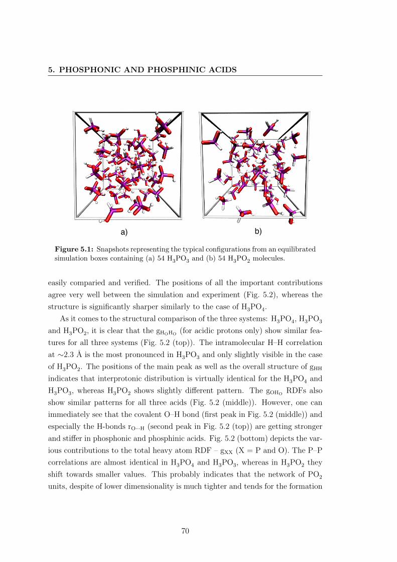
5. PHOSPHONIC AND PHOSPHINIC ACIDS
a) b)
Figure 5.1: Snapshots representing the typical configurations from an equilibratedsimulation boxes containing (a) 54 H3PO3 and (b) 54 H3PO2 molecules.
easily comparied and verified. The positions of all the important contributions
agree very well between the simulation and experiment (Fig. 5.2), whereas the
structure is significantly sharper similarly to the case of H3PO4.
As it comes to the structural comparison of the three systems: H3PO4, H3PO3
and H3PO2, it is clear that the gHOHO(for acidic protons only) show similar fea-
tures for all three systems (Fig. 5.2 (top)). The intramolecular H–H correlation
at ∼2.3 A is the most pronounced in H3PO3 and only slightly visible in the case
of H3PO2. The positions of the main peak as well as the overall structure of gHH
indicates that interprotonic distribution is virtually identical for the H3PO4 and
H3PO3, whereas H3PO2 shows slightly different pattern. The gOHORDFs also
show similar patterns for all three acids (Fig. 5.2 (middle)). However, one can
immediately see that the covalent O–H bond (first peak in Fig. 5.2 (middle)) and
especially the H-bonds rO···H (second peak in Fig. 5.2 (top)) are getting stronger
and stiffer in phosphonic and phosphinic acids. Fig. 5.2 (bottom) depicts the var-
ious contributions to the total heavy atom RDF – gXX (X = P and O). The P–P
correlations are almost identical in H3PO4 and H3PO3, whereas in H3PO2 they
shift towards smaller values. This probably indicates that the network of PO2
units, despite of lower dimensionality is much tighter and tends for the formation
70

5.1 Structural Properties
0 1 2 3 4 5 6 7 8
r, Å
0
1
2
3
4
5g X
X(r
)H3PO3, simulated 383 K
H3PO3, experiment 373 K
Figure 5.2: The full simulated radial pair distribution function gXX (where X =P, O and H) and gXX from the neutron scattering study.95
of linear chains, as was also anticipated from the study of the crystalline struc-
ture of H3PO2.72 Surprisingly, the intramolecular structure (P–O bonds; Fig. 5.2
(bottom)) does not show any pronounced changes between the three systems.
The gOO peak, which contains both the intramolecular and intermolecular con-
tributions slightly shifts in H3PO2 and suggests that the internal structure of
hypophosphite anion is more rigid than that of phosphite or phosphate anions,
whereas the covalent O-H strengths show an opposite trend.
Fig. 5.4 depicts the distribution of the H-bond geometries (lengths and angles)
for all three acid systems. The H-bond length markedly decreases in the series:
rOO ≈ (H3PO4) 2.60 A > rOO ≈ (H3PO3) 2.57 A > rOO ≈ (H3PO2) 2.52 A.
This increase in the H-bond strength is also pronounced in the distribution of
the donor–acceptor–proton angles. The extremely short H-bond in H3PO2 is
associated with a very low PT barrier and an appropriate account of the nuclear
quantum effects would probably make the bond symmetrical with respect to the
position of the proton.
71

5. PHOSPHONIC AND PHOSPHINIC ACIDS
0 3 4 7 8
0.0
0.5
1.0
1.5g H
OH
O(r
)
H3PO4
H3PO4
H3PO2
5
10
15
20
g OH
O(r
)
H3PO4
H3PO3
H3PO2
r, Å
0
5
10
15
20
25
g XX(r
) (X
=P,O
) P - P (H3PO4)P - O (H3PO4)O - O (H3PO4)P - P (H3PO3)P - O (H3PO3)O - O (H3PO3)P - P (H3PO2)P - O (H3PO2)O - O (H3PO2)
0 3 4 7 8
Figure 5.3: Radial pair distribution functions for the liquid H3PO4, H3PO3 andH3PO2. (top) gHOHO
only for the acidic protons (excluding the hydrogens cova-lently bonded to phosphorus). (middle) gOHO
for the acidic protons and oxygenatoms, the first peak comes form the covalent O–H bond and the second due to theH-bonding (H· · · O). (bottom) gXX, where X = P or O, shows the different heavyatom pair contributions.
72

5.2 Dynamical Properties
2 2.5 3 3.5RO-O, Å
0 25 50 75angle, deg
α
Figure 5.4: H-bond geometries for H3PO4 (black), H3PO3 (red) and H3PO2
(green): probability distributions for (left) RO...O distances, and αO−H...O angles.
5.2 Dynamical Properties
Similarly to the previous discussion on phosphoric acid, the next step in the elu-
cidation of the properties of the other two phosphorus oxoacids is the evaluation
of proton and molecular diffusion coefficients. Although, the proton conduct-
ing properties of H3PO4 and H3PO3 have already been experimentally estab-
lished,65,68 up to now little was known about the proton transport in H3PO2. For
this reason, a number of experiments were carried out on phosphinic acid and the
results are used to supplement the modeling work.66
The crystals of nominally dry phosphinic acid were obtained by vacuum dry-
ing (P=10−5 mbar) the aqueous solution (Sigma-Aldrich ∼50% aq.) using the
procedure described by Jenkins et al.178 Before the conductivity and self-diffusion
measurements, the acid crystals were additionally dried on a filter paper and af-
terwards transferred into gas-tight glass sample holders in an argon filled glove
box. The crystals were subsequently melted and a number of conductivity and
PFG-NMR measurements were performed at different temperatures on the liquid
sample.66 The experimental results for all three acids are presented in Fig. 5.5
73

5. PHOSPHONIC AND PHOSPHINIC ACIDS
and 5.6.
The experimentally measured conductivities together with the tracer diffusion
coefficients in phosphinic acid allow for the general picture of proton conduction
mechanism to be drawn. Although the conductivity of H3PO2 is significantly
lower than that of other acids (Fig. 5.6), it is still relatively high compared to
a wider class of H-bonded liquids. Moreover, there still exists an approximately
10% difference between proton and phosphorus diffusion coefficients, indicating
a contribution from structural diffusion to proton conductivity. Although, the
precise determination of this contribution is complicated without experimental
input for the degree of self-dissociation, one can still try to systematically include
the correlations in proton transport (Haven ratio (H)) from the knowledge of
H3PO4 and H3PO3. Two different limiting situations concerning the mechanism
of proton conduction in phosphinic acid can be assumed: first all the current
is carried out via structural diffusion with perfectly random motion of protonic
defects (H = 1) and second a completely vehicular nature of proton transport (H
= ∞). One can estimate the structural diffusion contribution from the Nernst-
Einstein relation using the difference of the two self-diffusion coefficients rather
than separately estimating the mobilities and concentrations of protonic defects:66
σstructureD ≈ F 2
RTc(HOH)(D(HOH)−D(HPH)) (5.1)
where σstructureD is the conductivity contribution of structural diffusion, D(HOH)
and D(HPH) the average self-diffusion coefficients obtained from 1H PFG-NMR
and c(HOH) the concentration of all acidic (HOH) protons. The advantage of
this procedure is the possibility to obtain the proton conductivities from tracer
diffusion coefficients without precise knowledge of the charge carrier concentra-
tions, assuming that the mobility of protonic defects and proton diffusion are
completely random (Haven ratio is unity) processes. For the case of completely
vehicular transport, one has to assume equal proton and molecular diffusion co-
efficients and by using the Nernst-Einstein equation:66
74

5.2 Dynamical Properties
σvehicleD =F 2
RT(c(H4PO
+2 )D(H4PO
+2 ) + c(H2PO
−2 )D(H2PO
−2 ))
≈ F 2
RT2αc(HPH)D(HPH) (5.2)
where c(HPH) is the phosphonic acid concentration (c(HPH) = ρ/MW ; ρ is the
density and MW the molecular weight of the phosphonic acid). Taking D(HPH) as
being identical with the H4PO+2 and H2PO−2 self-diffusion coefficients, one obtains
the degree of self-dissociation (α) in H3PO2 to be ∼5.6%. This α would explain
the experimentally measured total conductivity (σtotexp) by a completely vehicular
proton transport mechanism. However, this is not the case, since as mentioned
before, there is an approximately 10% difference between the experimentally ob-
tained D(HOH) and D(HPH) (Fig. 5.5). In the case of entirely structural diffusion
proton transport, the calculated σstructureD only accounts for approximately 60% of
the σtotexp, suggesting that in contrary to the other two acids, there is a substantial
vehicular contribution to proton conductivity in phosphinic acid. In this mech-
anism, we assumed that the Haven ratio is equal to 1, which is only the case of
perfectly random processes but deviates once the different correlations between
mobility of protonic charge carriers and proton diffusion appear. These devia-
tions are known to occur in various proton conductors.179 Knowing that Haven
ratios for phosphorus oxoacids are higher than unity and that the degree of cor-
relations increases from phosphoric (H ≈ 1.5) to phosphonic (H ≈ 2.5) acid, this
most probably must also hold for phosphinic acid. We believe that an assumption
of linearly increasing Haven ratio for all three acids would provide a reasonable
approximation, which could help to reveal the principle proton transport mecha-
nism in phosphinic acid. Taking H(H3PO2) ≈ 3.5, one can self-consistently solve
for α by estimating the total conductivity (σstructureD + σvehicleD ) and comparing it
to the experimental σtotexp until the two are equal:66
σtotexp ≈ σvehicleD + σstructureD
≈ F 2
RT(2αc(HPH)D(HPH) +
1
Hc(HOH)(D(HOH)−D(HPH))) (5.3)
75

5. PHOSPHONIC AND PHOSPHINIC ACIDS
Using this approximation, one obtains the degree of self-dissociation α ≈ 4.5%
which results in ∼21% of the current in phosphinic acid carried by proton struc-
tural diffusion (Fig. 5.6).66
As in any intrinsic proton conductor, self-dissociation is initiated by a PT
in an intermolecular H-bond and leading to the formation of a contact ion pair.
Before this pair is separated there is a high probability for the reverse process
to occur in strong low-barrier bonds. If a backward transfer occurs, the whole
process contributes neither to proton diffusion nor conduction. But if before
the proton is transferred back, the H-bond is broken through reorientation of the
newly formed defect and another exchangeable proton of the same species forms a
H-bond with the initial proton acceptor, this different proton may be transferred.
The latter process does then not lead to charge separation and hence conductivity,
but since the protons exchange their identity, it contributes to proton diffusion. It
is clear that the corresponding Haven ratio depends on the lifetime of the H-bond,
the probability for proton backward transfer and the number of exchangeable
protons of the protonic defect. In the case of e.g. H4PO+2 the latter is only two,
and if the process, as described above, involves two neighboring molecules only,
the maximum Haven ratio expected for very short H-bond life times should not
exceed a value of 2. Although, out of the three phosphorus oxoacids, H3PO2 has
the strongest H-bonds and the lowest hydrogen bond concentration, which leads
to the lowest viscosity, highest molecular diffusion and probably also the lowest
hydrogen bond lifetime. From this consideration a Haven ratio of ∼2 is feasible,
but if more than just two molecules (contact ion pair) were involved in cooperative
PTs, the Haven ratio may also be higher.66 Since at this stage it is difficult to
conclusively decide on this issue, without an independent determination of the
exact degree of self-dissociation, the transport data for H = 2 corresponding to
a degree of self dissociation of α ≈ 3.5 % and ∼38 % of the current carried via
proton structural diffusion mechanism are included in (Fig. 5.6).66
The evaluation of diffusion coefficients from the AIMD simulation is based
on the same procedure as in Eq. 4.1. The obtained mean square displace-
ment dependence versus time as well as calculated diffusion coefficients are pre-
sented in Fig. 5.7. The estimated and experimental values are summarized
and compared in Table 5.1. In the case of phosphonic acid the AIMD calcu-
76

5.2 Dynamical Properties
Figure 5.5: Proton and molecular diffusion coefficients determined by the PFG-NMR with respect to temperature.66
lated diffusion coefficients show a reasonably good agreement to the experimen-
tal ones obtained from the PFG-NMR. Surprisingly, D2HCPMD(H3PO3) is slightly
lower than D2HCPMD(H3PO4) and contradicts the experimental finding, whereas
DmolCPMD(H3PO3) is higher than Dmol
CPMD(H3PO4) (Fig. 5.7; Table 5.1) and com-
plies with the experimental results. This observation might indicate an artefact
of the simulation, which could possibly arise from different equilibration histo-
ries of two different simulations, since the same kinetic temperature was used in
both systems with different melting points (315 K (H3PO4) vs. 346 K (H3PO3).
Nevertheless, the expected decrease in the ratio of proton versus molecular dif-
fusion rates in the simulation of H3PO3 is observed: D2HCPMD/D
PCPMD (H3PO4) ≈
5.4 vs. D2HCPMD/D
PCPMD (H3PO3) ≈ 3.7. The simulated diffusion coefficients for
phosphinic acid confirm the experimental prediction of even higher proton dif-
fusion rate than in the case of other acids, as well as much higher hydrody-
77

5. PHOSPHONIC AND PHOSPHINIC ACIDS
Figure 5.6: Conductivities and the respective contributions due to structuraldiffusion in H3PO4, H3PO3 and H3PO2.66
namic background due to the molecular diffusion of PO2 species. Although the
estimated D2HCPMD and DP
CPMD show reasonably good agreement, similar to the
other two cases, their ratio is significantly deviating from the experimental ra-
tio (D2HCPMD/D
PCPMD (H3PO2) ≈ 1.56 vs. D
2HCPMD/D
PCPMD (H3PO2) ≈ 1.1). This
probably indicates the fact that even though the proton dynamics is rather well
described within this AIMD scheme, the treatment of the hydrodynamic motion of
the molecules is still incomplete due to the short simulation time, limited system
size, periodic boundary conditions or absence of the van der Waals interactions.
As was already discussed in the previous part on phosphoric acid, within
the Debye diffusive model, a rotational diffusion constant Drot can be evaluated
from the angular mean square displacement via the relation in Eq. 4.3. The re-
sulting mean angular displacements and the calculated Drot values are presented
78

5.3 Vibrational spectra
System D2HCPMD D
31PCPMD D
1HPFG−NMR D
mol(H−P)PFG−NMR
H3PO4 4.03 · 10−6 0.75 · 10−6 5.40 · 10−6 1.15 · 10−6
H3PO3 3.67 · 10−6 0.99 · 10−7 5.98 · 10−6 2.30 · 10−6
H3PO2 6.27 · 10−6 4.03 · 10−6 7.63 · 10−6 7.48 · 10−6
Table 5.1: Calculated and experimental diffusion coefficients at 383 K for phos-phonic and phosphinic acids.
in Fig. 5.8. The results are consistent with the notions already applied when
discussing the structure of H-bond networks and diffusion coefficients. The cal-
culated rotational diffusion coefficients are very similar for H3PO4 and H3PO3,
reflecting the similar finding for the molecular diffusion coefficients (Fig. 5.5).
The Drot(H3PO4) ≈ 0.00775 rad2·ps−1 and Drot(H3PO3) ≈ 0.0081 rad2·ps−1 are
∼2.5 times lower than Drot(H3PO2) ≈ 0.0207 rad2·ps−1, indicating a much more
pronounced rotational freedom in the latter system. Nevertheless, despite the fact
that phosphinic acid molecule, on average forms only two H-bonds, its molecular
rotational dynamics is still much slower (about one order of magnitude) than that
of water.159,160 This indicates that the very strong H-bonds present in H3PO2 are
strongly hindering the reorientation of molecules and their rotational freedom.
5.3 Vibrational spectra
In molecular dynamics simulations, the vibrational power spectrum of a classical
fluid can be estimated from the Fourier transformed ensemble averaged particle
velocity autocorrelation function:
Cvv(t) = 〈v(t) · v(0)〉 (5.4)
Cvv(ω) =1
2π
∫ +∞
−∞dt exp−iωtCvv(t). (5.5)
At this point it is important to note that the power spectrum obtained from
Eq. 5.5 carries no information about the IR or Raman activities or absorption
intensities and only gives the vibrational modes (including the anharmonic con-
tributions) of the system.
The vibrational spectra of all three acid systems are presented in Fig. 5.9.
79

5. PHOSPHONIC AND PHOSPHINIC ACIDS
0 2 4 6 8 10time, ps
0
1
2
3
4
5
<|r(t
)-r(0
)|2 >,
Å2
D(2H; H3PO4) = 4.03 · 10
-6 cm
2/s
D(31
P; H3PO4) = 7.51 · 10-7
cm2/s
D(2H; H3PO3) = 3.67 · 10
-6 cm
2/s
D(31
P; H3PO3) = 9.92 · 10-7
cm2/s
D(2H; H3PO2) = 6.27 · 10
-6 cm
2/s
D(31
P; H3PO2) = 4.03 · 10-6
cm2/s
Figure 5.7: The average angular displacement of the P–O bond with respect totime and the corresponding rotational diffusion constants for H3PO4, H3PO3 andH3PO2 at 383 K.
As one can see from Fig. 5.9, the frequency of the O–H stretching frequency is
significantly red-shifted as compared to its typical value in liquid water. This
shift is primarily due to the deuteration of the system (in comparison νOH ≈3500 cm−1 in H2O vs. νOD ≈ 2500 cm−1 in D2O) as well as the much stronger H-
bonding present in phosphorus oxoacids. The effect of the increasing strength of
the H-bonds is clearly manifested in the red-shift of the νOH vibration going from
D3PO4 (νOD ≈ 2450 cm−1) to D3PO3 (νOD ≈ 2200 cm−1) and D3PO2 (νOD ≈2000 cm−1). An identical trend was found by Leuchs and Zundel82 from the IR
spectra of the non-deuterated acids : νOH ≈ 3000 cm−1 (H3PO4), νOH ≈ 2900
cm−1 (H3PO3) and νOH ≈ 2650 cm−1 (H3PO2). The vibrations at 1750 cm−1
and 1700 cm−1 for H3PO3 and H3PO2 respectively, are the corresponding νPD
stretching modes and which are absent in the H3PO4 spectrum. In the Raman and
IR spectra,180,181 the peaks at ∼1100 cm−1 were identified as νP = O, symmetric
and asymmetric νs,asPO−n stretch frequencies. The peaks at ∼950 cm−1 (D3PO4),
∼940 cm−1 (D3PO3) and ∼880 cm−1 (D3PO2) correspond to νs,asPOD stretching
80

5.4 Proton Transfer Kinetics
time, ps
0
0.5
1
<θ
2>
DR (H
3PO
4) = 0.00775 rad2·ps-1
DR (H
3PO
3) = 0.0081 rad2·ps-1
DR (H
3PO
2) = 0.0207 rad2·ps-1
Figure 5.8: Average mean square displacements and corresponding diffusion con-stants as obtained from the Einstein relation for hydrogen and phosphorus atomsin H3PO4 at 383 K.
and δPOD bending modes. The rest of the modes at lower frequencies arise from
the O–P–O bending vibrations.
5.4 Proton Transfer Kinetics
In this section, the important time scales for the proton transfer and solvent
reorientation are extracted using the same population correlation function (PCF)
approach as described in Section 4.4. The obtained PCFs for H3PO3 and H3PO2
and their triexponential fits are shown in Figs. 5.10 and 5.11. In the case of
phosphonic acid, the obtained decay constants for the PCF including all proton
transfers (including rattling) are: τ1 = 0.275 ps, τ2 = 1.78 ps and τ3 = 7.37 ps. In
the case of phosphinic acid, the obtained decay constants for the PCF including all
proton transfers are: τ1 = 0.492 ps, τ2 = 2.32 ps and τ3 = 9.32 ps. Generally, the
three constants and especially their ratios for H3PO3 and H3PO2 are reminiscent
of the ones obtained for H3PO4, indicating that probably very similar mechanisms
81

5. PHOSPHONIC AND PHOSPHINIC ACIDS
0 500 1000 1500 2000 2500 3000 3500
wavenumber, cm-1
VD
OS
D3PO
4
D3PO
3
D3PO
2
Figure 5.9: Comparison of the vibrational power spectra for H3PO4, H3PO3 andH3PO2.
are governing the proton dynamics in all three acids. Identically to the case of
phosphoric acid the fast time constant represents the fast proton rattling, the
second τ2 corresponds to the fast response of the solvent (interprotonic coupling
and formation of Grotthuss chains) and the third, slowest to the complete H-
bond network reorganization. The results indicate that the time scales of the PT
reactions are not only strongly affected by the H-bond strength, but also by the
rotational and hydrodynamic background of the molecular system. Although the
overall process (∫Cc(t)dt) is becoming faster from phosphoric to phosphinic acid,
the individual constants corresponding to the build-up (τ2) and depolarization of
polarized chains (τ3) are slower in less tightly bound H-bond networks.
82

5.5 Proton Transfer Energetics
0.01 0.1 1 10 100time, ps
0
0.2
0.4
0.6
0.8
1
Cc(t
)
including rattling
excluding rattling
triexponential fits
Figure 5.10: Proton transfer population correlation functions (including and ex-cluding proton rattling) and their triexponential fits for H3PO3.
5.5 Proton Transfer Energetics
In Fig. 5.12 the free energy profiles along the asymmetric stretch coordinate δ
are presented. All the calculated ∆A[δ] show distinct double well character. As
mentioned in the previous chapter, the PT barriers are predominantly affected by
the most probable proton donor–acceptor separation, which is decreasing in a row
from phosphoric to phosphinic acid: rOO(H3PO4) > rOO(H3PO3) > rOO(H3PO2).
This trend is clearly reflected in the reduction of the PT barrier: ∼62 meV
(H3PO2) < ∼71 meV (H3PO3) < ∼80 meV (H3PO4). Nuclear quantum effects
might lower these barriers slightly, but as already noted, the effects are expected
to be small and the protons are undergoing transfer close to the full adiabatic
limit.182,183
83

5. PHOSPHONIC AND PHOSPHINIC ACIDS
0.01 0.1 1 10 100time, ps
0
0.2
0.4
0.6
0.8
1
Cc(t
)
including rattling
excluding rattling
triexponential fits
Figure 5.11: Proton transfer population correlation functions (including and ex-cluding proton rattling) and their triexponential fits for H3PO2.
5.6 The Structure and Energetics of Charged
Species
In this section the structure and energetics of protonic defects (species with carry-
ing excess and deficient protons) are analyzed. Identically to the analyses carried
out on phosphoric acid, each proton is formally assigned to its nearest neighbor
oxygen atom and subsequently to a particular PO3 or PO2 unit. After this as-
signment, one can even formally define the ‘degree of self-dissociation’ in each
acid. However, this kind of definition still includes all the transiently transfer-
ring protons, which do not contribute to the actual charge separation and self-
dissociation. One way to exclude these events and get a better estimate for the
degree of self-dissociation is to select a certain δ cut-off value and only count those
protons which are truly associated with a certain phosphate species, excluding
those transiently shared by two species. Protons with δ approaching 0 are be-
ing transferred, therefore one can select a certain value for |δcut−off | which selects
only those protons which are far from the PT transition state and can be unam-
biguously assigned to a particular PO4 unit. The results for two different δcut−off
84

5.6 The Structure and Energetics of Charged Species
-1.5 -1 -0.5 0 0.5 1 1.5δ, Å
0
0.02
0.04
0.06
0.08
0.1
0.12A
[δ],
eV
H3PO4
H3PO3
H3PO2
Figure 5.12: Free energy profiles A(δ) along the proton transfer coordinate δ forH3PO4, H3PO3 and H3PO2.
values: 0.0 A (all protons are unambiguously assigned to phosphate species) and
0.3 A (protons close to the PT transition state are excluded), are presented in
Table. 5.2. These values correspond to the fractions of HnPOyx species having
uncompensated protonic charge (excess or deficient protons). Although, this ap-
proach to estimate the charge carrier concentration is rather crude, it still shows
some interesting features, which can be compared to the available experimental
data. The only available experimental value of this property is that for phosphoric
acid: ∼7.4%. From Table. 5.2, one can see that the charge carrier concentration
is systematically decreasing from H3PO4 to H3PO2. This reflect the previously,
discussed finding that even though the proton mobility is increasing from H3PO4
to H3PO2, the measured conductivities show an opposite trend and suggest that
the effective charge carrier concentration is significantly reduced. Nevertheless,
the simulated values are still in a reasonably well agreement, especially if the
transiently shared protons are excluded from the analysis.
The next question addressed in this section is: what is the extent of the H-
bond network contraction around the regions carrying excess protonic charge in
85

5. PHOSPHONIC AND PHOSPHINIC ACIDS
δcut−off , A H3PO4 H3PO3 H3PO2
0.0 A 25.6 % 20.1 % 8.1 %
0.3 A 11.3 % 7.5 % 1.9 %
Table 5.2: Calculated fractions of molecules with uncompensated protonic charge(having excess or deficient protons) for H3PO4, H3PO3 and H3PO2 systems anddifferent proton assignment criteria δcut−off .
H3PO3 and H3PO2? The calculated gOO(r) RDFs for phosphonic and phosphinic
acids with respect to the protonation of POx species are presented in Figs. 5.13
and 5.14. Identically to the case of phosphoric acid, the other two acids also
feature a marked contraction of the H-bond network around the positive defects.
In H3PO3 for instance: rOO(H4PO+3 ) ≈ 2.47 A < rOO(H2PO−3 ) ≈ 2.53 A <
rOO(H3PO3) ≈ 2.55 A (Fig. 5.13) and the running coordination numbers of the
first solvation shell of each species: nOO(H4PO+3 ) ≈ 3.2 < nOO(H3PO3) ≈ 4.0 <
nOO(H2PO−3 ) ≈ 5.1 (Fig. 5.13). In the case of H3PO2: rOO(H4PO+2 ) ≈ 2.44 A <
rOO(H2PO−2 ) ≈ 2.46 A < rOO(H3PO4) ≈ 2.51 A and the running coordination
numbers: nOO(H4PO+2 ) ≈ 2.0 < nOO(H3PO2) ≈ 2.0 < nOO(H2PO−2 ) ≈ 2.6
(Fig. 5.14). The results show that all three acid systems show a similar shortening
of H-bonds in the vicinity of charged species, the most severe being around the
region having an excess number of protons. Phosphoric and phosphonic acids
show an equivalent asymmetry of their solvation shells, with H4PO+x displaying
undercoordination and H2PO−x a noticeable overcoordination. Although, H3PO2
features the same trend in the H-bonding strength (just the least pronounced), its
solvation asymmetry is not visible anymore. This could be explained by the fact
that contrary to phosphoric and phosphonic acids or even water, phosphinic acid,
already, has an excess number of proton acceptor sites and even nominally neutral
species are on average undercoordinated (only one acceptor site occupied).
It is also interesting to look at the PT energetics around the H4PO+x and
H2PO−x species. The PT free energy profiles calculated using the same procedure
as in Eq. 4.8 taking into account only those protons belonging to the charged de-
fects are shown in the Fig. 5.15 and 5.16. In both cases, the computed free energy
profiles show very similar trends as those of H3PO4: the PT barrier around the
positive ion is the lowest and the one for the protons in the vicinity of a negative
86

5.7 On the Degree of Protonation
site in between the ‘positive’ and ‘overall’ PT barrier heights. The PT barriers for
H4PO+x ·(H3PO4)n in phosphonic and phosphinic acid systems are significantly be-
low the average thermal energy of the simulation with H3PO2 showing an almost
single well PT potential (Fig. 5.16) for protons bound by H4PO+2 . The latter
behavior in the case of aqueous protonic defect simulations becomes apparent
only after introducing appropriate treatment of nuclear quantum effects.9,167
2 2.5 3 3.5 4r, Å
0
1
2
3
g OO(r
) / n
OO(r
)
gOO(r) - H3PO3 · (H3PO3)n
gOO(r) - H4PO3+ · (H3PO3)n
gOO(r) - H2PO3- · (H3PO3)n
nOO(r) (neutral)
nOO(r) (positive)
nOO(r)
Figure 5.13: gOO and running coordination numbers (nOO) of oxygen atoms forH3PO3 in its various states of protonation.
5.7 On the Degree of Protonation
In this section the properties of the H-bond networks of phosphonic and phos-
phinic acids are discussed. As already mentioned in the previous chapter, it is
only the phosphoric acid, which has an excess ratio of proton donor versus accep-
tor sites resulting in frustrated H-bond network. The importance of this property
for the overall proton transport mechanism was underlined in the discussion of
proton transport mechanism in H3PO4. The approach involved here is identical
to the one used in Section 4.7. The parameters in Eq. 4.9 were fine-tuned in the
87

5. PHOSPHONIC AND PHOSPHINIC ACIDS
2 2.5 3 3.5 4r, Å
0
1
2
3
4
g OO(r
) / n
OO(r
)
gOO(r) - H3PO2 · (H3PO2)n
gOO(r) - H4PO2+ · (H3PO2)n
gOO(r) - H2PO2- · (H3PO2)n
nOO(r) (neutral)
nOO(r) (positive)
nOO(r) (negative)
Figure 5.14: gOO and running coordination numbers (nOO) of oxygen atoms forH3PO2 in its various states of protonation.
same way as in the case of phosphoric acid in order to reproduce the average oxy-
gen protonations of 0.67 and 0.5 in phosphonic and phosphinic acids, respectively.
From Fig. 5.17, one can immediately see that all oxygen atoms form a contin-
uous population of various H-bond configurations with respect to their degree
of protonation. The bond-order distribution curves for oxygen populations show
very similar structure for all three acid systems (Fig. 5.17). The reduction of the
fraction of proton donors in the H-bond networks is manifested by the shift of the
first peak towards even lower oxygen protonations in phosphonic and phosphinic
acids. The same trend is observed in the proton donating oxygen peaks as well.
However, the profiles still indicate a significant presence of oxygens with a higher
than unity protonation. The latter indicates that even in these “non intrinsically
frustrated” H-bond networks, the situations where an already proton donating
oxygen accepts another H-bond are forming due to the dynamic disorder. The
latter was also anticipated by Leuchs and Zundel from the appearance of a shoul-
der in the νOH IR absorption band of liquid H3PO3 and H3PO2. Moreover, in
the case of H3PO2 (Fig. 5.17 (blue line)) the presence of these sites even results in
a finite concentration of non-protonated oxygen atoms (blue curve is not equal to
88

5.8 Interprotonic Coupling
-1.5 -1 -0.5 0 0.5 1 1.5δ, Å
0
0.025
0.05
0.075
0.1
0.125
A[δ
], eV
H3PO3 (all protons)
H4PO3+ · (H3PO3)n
H2PO3- · (H3PO3)n
Figure 5.15: Free energy profiles A(δ) along the proton transfer coordinate δ forH3PO3, H4PO+
3 and H2PO−3 .
0 for∑ni = 0). In principle these frustrated configurations must play a similar
role as in H3PO4 by facilitating the efficient solvent depolarization and dielectric
relaxation and give rise to proton conductivity. The actual mechanisms are more
thoroughly addressed in the following sections.
5.8 Interprotonic Coupling
The proton dynamics in phosphonic and phosphinic acid is characterized by an
even more pronounced rattling of protons than in phosphoric acid, which mainly
arises from the presence of stronger H-bonds (Sec. 5.4). For the case of phosphoric
acid we already proved that a dynamical response mainly driven through the
electrostatic proton-proton interaction accompanies the PT events, leading to
correlated PTs and the formation of polarized chains spanning several molecular
lengths. In this part, the same kind of methodology and line-of-thought is followed
to address these questions for the other two acid systems.
Figs. 5.18 and 5.19 depict the gHH RDFs resolved in r and δ, containing infor-
mation about the spatial distribution of protons with respect to their position in
89

5. PHOSPHONIC AND PHOSPHINIC ACIDS
-1 -0.5 0 0.5 1δ, Å
0
0.025
0.05
0.075
0.1
0.125
A[δ
], eV
H3PO2 (all protons)
H4PO2+ · (H3PO2)n
H2PO2- · (H3PO2)n
Figure 5.16: Free energy profiles A(δ) along the proton transfer coordinate δ forH3PO2, H4PO+
2 and H2PO−2 .
the H-bond (δ). As one can see, both systems feature a significant response of the
protonic subsystems upon the PT process. The gHH(r, δ) for the case of H3PO3
clearly resembles the one calculated for H3PO4 (Fig. 4.13). In phosphonic acid,
only the position of the main peak is slightly shifted towards larger separations
(3.5 A vs. 3.9 A), reflecting the lower average density of protons. Nevertheless,
the main peak at ∼3.9 A in H3PO3 increases for δ → 0 in a similar fashion as in
H3PO4. The calculated gHH(r, δ) for phosphinic acid, clearly exhibits a different
pattern from those found for the other two systems. In this case, the main peak
is much more diffuse and does not show a significant variation in height with
respect to δ. However, the position of the main peak is significantly shifted to-
wards shorter proton-proton separations (onset shifts from ∼4.0 to ∼3.7 for δ →0). This shift most probably, can be explained by stronger contraction of the H-
bonds around the species carrying excess protonic charges in H3PO2 (Fig. 5.14),
as well as the fact that the overall density of protons is significantly lower (there
is on average only one proton per PO2 species).
In principle, these results suggest that PTs are obviously strongly correlated to
the dynamics of surrounding protons these two acids (especially in H3PO3) as well.
90

5.9 On the Formation of Grotthuss Chains and Proton ConductionMechanisms
0 0.5 1 1.5
0
0.05
0.1
0.15
H3PO
4
H3PO
3
H3PO
2
∑ni
Probability
OverprotonatedUnderprotonated
Figure 5.17: The probability distribution of various oxygen protonation statesdefined as the sum of individual bond-orders due to surrounding protons (
∑ni).
In the following section, the questions whether this behavior can lead to several
correlated PTs and the formation of extended polarized chains is addressed.
5.9 On the Formation of Grotthuss Chains and
Proton Conduction Mechanisms
It was previously described that special configurations forming in phopshoric acid
due to interprotonic coupling could seed up the formation of extended Grotthuss
chains without a significant solvent reorganization at slow dipolar level. Concern-
ing this process in H3PO3 and H3PO2 on a qualitative level, there are obviously
two effects competing for and against the formation of extended polarized chains:
stronger and shorter H-bonds should result in an even more pronounced protonic
polarization, whereas stronger dynamical background and dipolar nature of the
medium (µgasH3PO3 ≈ 1.5 D and µgasH3PO2 ≈ 2.5 D) should disrupt this pro-
cess. The possibility of mutual protonic polarizability and correlated motion in
91

5. PHOSPHONIC AND PHOSPHINIC ACIDS
1.0 2.0 3.0 4.0 5.0 6.0 7.0 8.00.0
0.2
0.4
0.6
0.8
1.0
1.2
1.4
1.6
0
0.2
0.4
0.6
0.8
1
1.2
1.4
1.6
r,
δ,
gHH
(r,δ)
Å
Å
δeq
~ 0.59 Å
Figure 5.18: gHH(r, δ; H3PO3) radial distribution function resolved in r and δ,containing information about the spatial distribution of protons with respect to δ(δeq is the equilibrium value in the simulation).
extended molecular aggregates in these two acid systems was also suggested by
Leuchs and Zundel in their IR study.82
AIMD simulations enable the determination of existence and average length
of extended Grotthuss chains. In order to extract these quantities for phosphonic
and phosphinic acid systems the same correlation function approach developed
in Sec. 4.9 is employed. The calculated proton coupling correlation functions
C(n)(H3PO3) and C(n)(H3PO2) are presented in Fig. 5.20. The probability of
forming extended Grotthuss chains in phosphonic and phosphinic acids increases
with time; for an increment of τres = 50 fs, Fig. 5.20 indicates ∼10% probability
for forming a Grotthuss chain of four phosphite or hypophosphite species con-
nected by three H-bonds (see also Fig. 5.21 (a)). Clearly, the degree of coupling
between the protons within the neighboring H-bonds is significantly reduced, de-
spite the stronger H-bonds and lower concentration of frustrated sites which also
contribute to the destructive solvent response on the formation of chains compris-
ing polarized H-bonds. Interestingly, both H3PO3 and H3PO2 show an almost
identical decay of C(n) for protons n H-bonds away from each other, with H3PO3
92

5.9 On the Formation of Grotthuss Chains and Proton ConductionMechanisms
1.0 2.0 3.0 4.0 5.0 6.0 7.00.0
0.2
0.4
0.6
0.8
1.0
1.2
1.4
1.6
0
0.2
0.4
0.6
0.8
1
1.2
r,
δ,
gHH
(r,δ)
Å
Å
δeq
~ 0.52 Å
Figure 5.19: gHH(r, δ; H3PO2) radial distribution function resolved in r and δ,containing information about the spatial distribution of protons with respect to δ(δeq is the equilibrium value in the simulation).
showing slightly higher probability for forming chains of three H-bonds and faster
decay in the probability to form longer ones. The important point is that the
probabilities for Grotthuss chain formation in H3PO3 and H3PO2 beyond three
H-bonds are significantly lower than in H3PO4 and their slight variations can be
attributed to the statistical noise present in the simulations.
Identically to the case of phosphoric acid, these chains are terminated by the
H2PO−3−2 and H4PO+3−2 species. The latter can more easily propagate through
the H-bond network (Figs. 5.15 and 5.16; Fig. 5.21 (a) and (b)), while the former
are less mobile. In order to complete the charge separation/self-dissociation,
the central part of the polarized H-bonded chain connecting both defects must
be depolarized, as has been previously emphasized for the self-dissociation of
phosphoric acid (Sec. 4.10) or water.177 Without this depolarization, the charge
separation can be easily reversed through the intact chain. The depolarization
must take place in the center of the chain, since the terminal H-bonds already have
the proper orientation with respect to the terminating charges. At first glance, it
might seem that the presence of even stronger H-bonds in these systems would
93

5. PHOSPHONIC AND PHOSPHINIC ACIDS
0 1 2 3 4 5 6 7 8 9n, connectivity
0
0.2
0.4
0.6
0.8
1
Pro
babili
ty
H3PO
4
H3PO
3
H3PO
2
Figure 5.20: Proton coupling correlation function Cpc(n) as a function of connec-tivity n. Only the H-bonds with δ ≤ 0.1 A (∼ 2.0% of the total number for H3PO3
and ∼ 3.5% for H3PO2) are considered as undergoing PT. The time increment τressets the finite relay time for the system to respond to correlated PTs (τres = 50 fs).
prevent efficient solvent reorientation processes. In the case of H3PO4, which has
a very peculiar H-bond network topology, the solvent reorganization is facilitated
by the intrinsic presence of frustrated sites. However, as is shown later and
was already predicted by Leuchs and Zundel in their IR study, the ”less strongly
bound OH groups” are able to form transiently due to the liquid disorder and their
concentration increases from phosphinic to phosphoric acid (see also Sec. 5.7). As
is shown later, the formation of ‘frustrated’ sites, where the same oxygen atom
simultaneously acts as a donor and an acceptor, in H3PO3 and H3PO2 essentially
plays the same role in the solvent reorientation process as in H3PO4 (Fig. 5.21).
Solvent relaxation (depolarization) is initiated when one of the solvent H3PO3−2
molecules forms a new H-bond by donating a proton to an oxygen atom in the
chain (Fig. 5.21 (c)). This proton is transiently transferred to the new accep-
tor (Fig. 4.17 (c)), which causes a strong coupling to the original H-bond in the
chain. In this way, the original H-bond is effectively weakened since the same
94

5.9 On the Formation of Grotthuss Chains and Proton ConductionMechanisms
oxygen atom must simultaneously be a proton donor and acceptor. This weak-
ened H-bond can easily break and, through a rapid torsional rotation around the
P–O bond axis, reorient, forming a new H-bond with a less acidic (protonated)
oxygen in the surrounding solvent molecules (Fig. 5.21 (d)). This relaxation com-
pletes the charge separation, and subsequent PTs close to charged species (mostly
H4PO+3−2) can be considered already a part of the “independent”migration of
these charged species. The latter process does not hinder the formation of new
chains and reorientation of solvent molecules until the oppositely charged species
meet, leading to a neutralization step. Mechanistically, this neutralization event
is again simply the complement of the self-dissociation process.
Obviously, the main features of the proton transport mechanism in phosphonic
and phosphinic acids are similar to those already described for phosphoric acid.
Nevertheless, the systematic changes in molecular properties of these systems
also result in pronounced differences at the macroscopic level. The increasingly
stronger H-bonds and protonic polarizabilities in H3PO3 and H3PO2 compensate
for the stronger dynamical background and dipolar coupling resulting in forma-
tion of extended Grotthuss chains, which are only slightly shorter than those in
the case of H3PO4. Although, H3PO3 and H3PO2 do not posses the intrinsically
frustrated H-bond networks, the situations where the same oxygen atoms must
act as proton donors and acceptors, form due to the disorder in protonic and
molecular subsystems. The importance for these sites for the solvent depolar-
ization and in turn for the overall stability and mobility of protonic defects was
emphasized for all three acid systems. Their concentration decreases in a row
from phosphoric to phosphonic to phosphinic acid and follows the trend observed
for the proton conductivities. This means that although the correlated proton
transfers and formation of polarized chains are essential ingredients for the emer-
gence of intrinsic transport of protonic defects, the efficient solvent reorientation
is no less important.
95

5. PHOSPHONIC AND PHOSPHINIC ACIDS
a)
-
+δ
+δ-δ
b)
-δ
+
d)
+δ
-δ+δ
-δ
+δ
+δ-δ
-δ
c)
- +
+-
+
S
-
- +
S
+
S
-
+δ
+δ-δ +
Figure 5.21: Snapshots of the elementary the proton structural diffusion steps inH3PO2. The schemes bellow the molecular structures show the ions and interchaindipole orientations, with the solvent being represented by a generalized coordinate~S. The charged ion pair is indicated with (+) and (-), the partial charges on theoxygen atoms are marked by +δ and −δ. The arrows denote the proton hops andmolecular reorientations.
96

6
Phosphoric acid and water
mixtures
In this chapter the results of AIMD simulations on phosphoric acid and water
mixtures are presented. Two systems corresponding to different phosphoric acid
– water ratios were chosen: the first one represents the intrinsic condensation
equilibrium existing in neat phosphoric acid (50 H3PO4 molecules + 2 H4P2O7
molecules + 2 H2O, System I), the second one – 85% wt. commercially available
phosphoric acid electrolyte (36 H3PO4 molecules + 36 H2O molecules, System
II). Two microcanonical runs of 25 and 50 ps were obtained for System I and
System II, respectively. The structure and dynamics of water in mixtures with
phosphoric acid is an intriguing problem since water is the only “dopant” which
does not disrupt the H-bond network of phosphoric acid and does not destroy
its ability to transport protonic charge carriers. System I was selected in order
to investigate the very low concentration of water molecules and their acid-base
equilibria, present in nominally dry phosphoric acid. The H3PO4 and water mix-
tures are not only interesting from a fundamental point of view, but are also
relevant for understanding the biological role of phosphates, which are always in
equilibrium with surrounding water,184 or even the proton transport mechanisms
on the surface of phospholipid bilayers.185–188 The discussion in this chapter is
started by evaluating the structural and dynamical properties from the simula-
tions and comparing them to the experimental data available in the literature.
97

6. PHOSPHORIC ACID AND WATER MIXTURES
Afterwards, a number of experimentally unavailable properties are estimated. Fi-
nally the discussion is turned towards the structure and transport mechanisms
of protonic defects. A snapshot from an equilibrated simulation of System II is
presented in Fig. 6.1.
Figure 6.1: A snapshot of a typical configuration from an equilibrated simulationbox containing 36 H3PO4 and 36 H2O molecules.
6.1 Structural Properties
The discussion of the phosphoric acid – water mixtures is commenced by evaluat-
ing the radial pair distribution functions and comparing them to the experimental
data, available in the literature.189 The simulated and experimental total RDFs
(gXX) for System II are presented in Fig. 6.2. The general shape of the two curves
agrees very well, however the two RDFs are shifted with respect to each other, the
experimental gXX indicates slightly weaker bonds. Surprisingly, all bonds lengths
obtained from the simulation show a systematic, equally strong, deviation from
the experimental data. Since, the systems described in the previous chapters of
98

6.1 Structural Properties
this work, show a much better agreement to the neutron scattering data, it is pos-
sible that this shift could be an artifact of the post-experimental data treatment
procedures.189 Moreover, the structure factors obtained by X-ray and neutron
scattering experiments in the same study also show significant discrepancies.189
0 1 2 3 4 5 6 7 8r, Å
0
1
2
3
4
5
6
7
8
g XX(r
)
(D3PO4)0.50(D2O)0.50, simulation at 383 K(D3PO4)0.53(D2O)0.47, experiment 298 K
Figure 6.2: The total simulated radial pair distribution function gXX (black)(where X = P, O and H) and gXX (red) from the neutron scattering study ofKameda et al.189
Fig. 6.3 shows the contributions of various atom pairs to the total RDF. Most
of the results correspond to System II, and only the important features of System
I, e.g. representing the coordination of water molecules, are depicted. Fig. 6.3
(top) shows the gHH(System II) superimposed with gHH(H2O) and gHH(H3PO4).
The first peak at 1.55 A is a contribution from the intramolecular H–H of water
molecules, the second one at ∼2.2 A comes from the two hydrogen atoms form-
ing two H-bonds with the same acceptor oxygen atom of the phosphate, and the
third one at ∼3.65 A is due to the hydrogen atom located on the same phosphate
unit. An important feature of the gHH(System II) (Fig. 6.3 (top)) is the shifting
and lowering of the second peak as compared to pure water, indicating that, on
99

6. PHOSPHORIC ACID AND WATER MIXTURES
average, the H-bonds are stronger in System II and water molecules are accepting
fewer H-bonds (a significant fraction of H2O molecules are in H3O+ state). The
gOH (Fig. 6.3 (middle)) reveals an even more interesting feature of the H-bonding
in H3PO4–H2O systems: the overall structure of gOH(System II) is virtually iden-
tical to gOH(H3PO4) (gHH(H2O) is given for comparison). This indicates that
H-bonds (the second peak in gOH) in System II are much stronger than those of
water and essentially as strong as those of phosphoric acid, although if one tries
to evaluate the volume contraction by comparing the experimental densities of
System II (ρ = 1.680g/cm3) and pure H3PO4 (ρ = 1.885g/cm3), there is only a
∼2% deviation from the ideal mixing. These features and especially the H-bond
strength suggest that general proton dynamics as well as proton transport mech-
anisms in these systems should be much more similar to those in phosphoric acid
than to those in water. The origin for this observation must lie in the electro-
statics of the system: although the acidities of the systems are not so different, a
significant fraction of water molecules must be in hydronium state and contract
the H-bond networks in their vicinity. The same trends are visible in the heavy
atom correlation functions gXX (Fig. 6.3 (bottom)). The P–O, OP,W–OP,W (H-
bonds) are identical in System II and neat H3PO4 and different from the pure
water peaks. The individual contributions to gOO show pronounced differences
between System II and water as well, e.g. gOwOw(System II) is shifted towards
lower values whereas gOPOW(System II) and gOPOP
(System II) show similar
bonding strengths as gOO(H3PO4). Furthermore, only a very slight difference
is seen between the average phosphate separation between System II and phos-
phoric acid (gPP in Fig. 6.3 (bottom)). All these observations suggest that the
molecular and especially the H-bond structure of phosphoric acid solution, even
at the 50% mol. water concentration, is virtually unperturbed by the presence of
water molecules. This strongly implies that the analysis of the molecular details
of proton transport mechanisms in these systems must follow the same line of
thought as previously developed for three neat phosphorus oxoacids.
100

6.1 Structural Properties
0 3 4r, Å
1
2
3
g HH(r)
H3PO4 + H2O (1:1 mixture)H2O (pure)H3PO4 (pure)
123456
g OH(r)
H3PO4 + H2O (1:1)H2OH3PO4gOwH (H3PO4 + H4P2O7 + H2O)
0246810
g XX(r)
(X=P
, Op, O
w) P - P (H3PO4 + H2O (1:1))P - P (H3PO4)Op - Op (H3PO4 + H2O)Op - Ow (H3PO4 + H2O)Ow - Ow (H3PO4 + H2O)O - O (H3PO4)O - O (H2O)P - Ow,p (H3PO4 + H2O)P - O (H3PO4)Op - Ow (H3PO4 + H4P2O4 + H2O)
0 3 4r, Å
Figure 6.3: Radial pair distribution functions of the H3PO4 water solutions. Thestructure of neat H3PO4 and H2O are given for comparison. (top) gHH for SystemII, H3PO4 and H2O. (middle) gOH for for System I, System II, H3PO4 and H2O; thefirst peak comes form the covalent O–H bond and the second due to the H-bonding(H. . . O). (bottom) gXX, where X = P or O, shows the different contributions fromheavy atom pairs to the total RDF.
101

6. PHOSPHORIC ACID AND WATER MIXTURES
6.2 Dynamical Properties
Now that the main structural properties of phosphoric acid – water system have
been established, this section deals with the dynamical properties of these sys-
tems. The proton diffusion and conductivity of phosphoric acid – water system
in a broad concentration range has already been addressed in a number of exper-
imental studies.69,79,190 The AIMD simulated diffusion coefficients in System II
were evaluated by Eq. 4.1. The calculated time dependence of the mean square
displacements for phosphorus, hydrogen and oxygen (in H2O) atoms are pre-
sented in Fig. 6.4. Before starting the discussion of the results, it is important to
mention that all of the experimental studies in these systems so far, only mea-
sured the D(1H) and D(31P ) diffusion coefficients and the separate measurement
of D(17O), which could rigorously establish the relation between the vehicular
and structural contributions to diffusion processes, is not yet available for any
phosphoric acid based proton conducting system. As indicated in Fig. 6.4, the
CPMD calculated proton diffusion constant (D2HCPMD = 4.22 · 10−6 cm2/s) is in a
relatively good agreement to the experimental value (D2Hexp (383 K) ≈ 7.5 · 10−6
cm2/s). A similar agreement is found for phosphorus diffusion coefficient (D31PCPMD
(383 K) = 1.2 · 10−6 cm2/s vs. D31Pexp (383 K) ≈ 4.0 · 10−6 cm2/s),79,190 despite
very limited statistics and finite size effects.
A simple way for estimating the contribution due to structural diffusion in Sys-
tem II, can be achieved by taking the proton diffusion coefficient (D(H)(System
II)) and subtracting the contributions from the individual vehicles (in this case
the diffusion coefficients of water DH2O(O) and phosphorus DH3PO4(P )):
Dstr(H) = D(H)− xDH2O(O)− (1− x)DH3PO4(P ) (6.1)
where x represents the fraction of protons attached to water. In the case of
System II x = 2/5 (two out of five protons are located on the water molecule).
For System II, Dstr(H) = 0.021 A2/ps, whereas in the case of neat phosphoric
acid (x = 0) Dstr(H) = 0.032 A2/ps (assuming that H3PO4 is a system with
100% structural diffusion). In 50% mol. phosphoric acid solution, this results in
∼66% of the proton diffusion coming from structural diffusion.
As previously mentioned, the experimental confirmation for this fact can not
102

6.2 Dynamical Properties
be fully confirmed without the 17O tracer diffusion experiments. Nevertheless,
one can roughly try to estimate whether the substantial increase in the conduc-
tivity of phosphoric acid upon dilution can be explained by simple hydrodynamic
arguments. One way of calculating whether this contribution can account for the
∼2-2.5 times increase in conductivity (System II: σ(333K) ≈ 0.25 S/cm; H3PO4:
σ(333K) ≈ 0.1 S/cm ) is to assume a completely vehicular contribution of water
to the proton transport (protons are carried as part of H3O+ species and do not
undergo any intermolecular PT). The viscosity of the 85% wt. phosphoric acid
solution shows a ∼5 fold decrease compared to 100% neat phosphoric acid. At
first, let’s assume that the diffusivity of H3O+ is approximately twice as large as
the one of the phosphate (species size consideration): D(O) = 2 ·D(P ). The sec-
ond necessary assumption is that of the fraction of molecules in H3O+ state, if one
considers that ∼50% of the water molecules are hydronium ions, the theoretical
(Nernst-Einstein) contribution to conductivity would be ∼0.024 S/cm. Even with
these severe assumptions, implying very different acidities of water and phospho-
ric acid, the increase in conductivity can not be explained by purely vehicular
arguments, suggesting that proton structural diffusion still plays an important
role in the conduction mechanism of these systems. The microscopic details of
the structural diffusion in System II, as obtained from the AIMD simulations, are
discussed in the following sections.
The computed vibrational spectrum of System II only confirms the general
picture of H-bonding, suggested by the analysis of the RDFs. The main features
in the vibrational power spectra of System II are virtually identical to those
obtained for neat H3PO4 (Fig. 6.5). The frequencies of the principal vibrational
modes in the two systems are only slightly shifted with respect to each other.
Only the ν(OD) is slightly broadened and shifted to higher frequencies, mainly
due to the presence of more diverse and weaker D2O−D2O H-bonds.
103
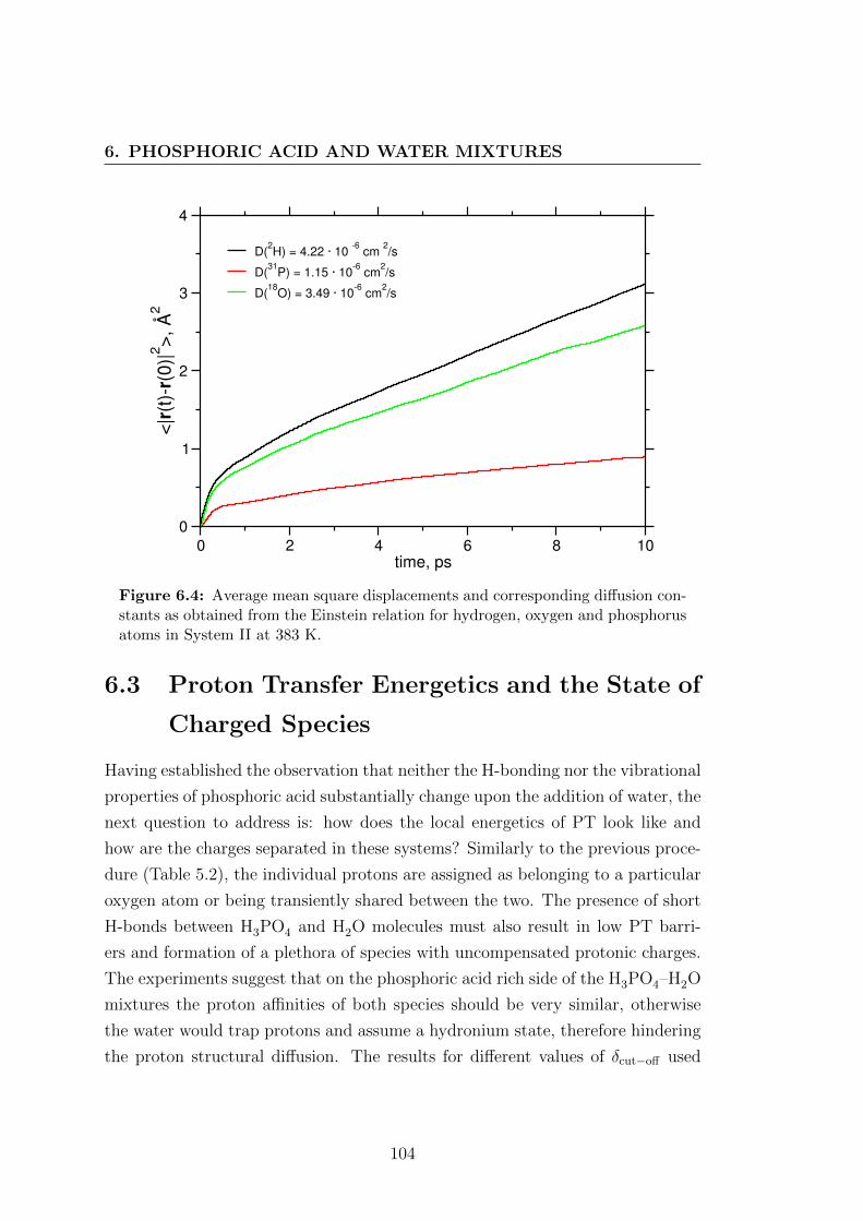
6. PHOSPHORIC ACID AND WATER MIXTURES
0 2 4 6 8 10time, ps
0
1
2
3
4
<|r(t
)-r(0
)|2 >,
Å2
D(2H) = 4.22 · 10
-6 cm
2/s
D(31
P) = 1.15 · 10-6
cm2/s
D(18
O) = 3.49 · 10-6
cm2/s
Figure 6.4: Average mean square displacements and corresponding diffusion con-stants as obtained from the Einstein relation for hydrogen, oxygen and phosphorusatoms in System II at 383 K.
6.3 Proton Transfer Energetics and the State of
Charged Species
Having established the observation that neither the H-bonding nor the vibrational
properties of phosphoric acid substantially change upon the addition of water, the
next question to address is: how does the local energetics of PT look like and
how are the charges separated in these systems? Similarly to the previous proce-
dure (Table 5.2), the individual protons are assigned as belonging to a particular
oxygen atom or being transiently shared between the two. The presence of short
H-bonds between H3PO4 and H2O molecules must also result in low PT barri-
ers and formation of a plethora of species with uncompensated protonic charges.
The experiments suggest that on the phosphoric acid rich side of the H3PO4–H2O
mixtures the proton affinities of both species should be very similar, otherwise
the water would trap protons and assume a hydronium state, therefore hindering
the proton structural diffusion. The results for different values of δcut−off used
104

6.3 Proton Transfer Energetics and the State of Charged Species
0 500 1000 1500 2000 2500 3000 3500
wavenumber, cm-1
VD
OS
D3PO
4
D3PO
4 + D
2O (1:1)
Figure 6.5: Vibrational spectrum for System II (H3PO4 + H2O (1:1)) (blue) andH3PO4 (black).
to count or exclude the transiently shared protons in System II are presented in
Table 6.1. The data summarizes the fractions of H3PO4 and H2O molecules with
respect to their state of protonation. Using the strict δcut−off = 0 A criterion, one
can immediately see that the degree of self-dissociation of the phosphoric acid
molecules is reduced in System II (see Table 5.2 for comparison), however ap-
proximately 12% of the water molecules are in the Eigen-like ion form. Basically,
this shows that the overall charge carrier concentration is very close to that of
pure H3PO4. If one assumes a stricter δcut−off criterion (e.g. δcut−off = 0.3 A),
the concentration of positively charged species is decreased, whereas the concen-
tration of negatively charged species increases. This indicates that a significant
fraction of the protons also are in Zundel-like forms, i.e. transiently shared be-
tween water and phosphoric acid molecules and suggesting that PT barriers in
acid-water H-bonds are very low. In the case of similar proton affinities of the two
species, another important aspect of this analysis is the possibility of phosphoric
105

6. PHOSPHORIC ACID AND WATER MIXTURES
δcut−off H4PO+4 H2PO−4 H3O+ OH−
0.0 A 7.5 % 19.0 % 12.0 % 0.0026 %
0.3 A 2.5 % 34.1 % 5.2 % 7.1 %
Table 6.1: Calculated fractions of water and phosphoric acid molecules in theirdifferent states of protonation in System II, with different proton assignment cri-terion δcut−off .
acid abstracting a proton from water and forming a hydroxide ion. However,
the results (Table 6.1) show that with δcut−off = 0 Aonly a very tiny fraction
of water molecules are in a probably, short-lived Zundel-like OH− form. Never-
theless, if the δcut−off value is increased up to 0.3 A a significant fraction of the
protons assigned to water molecules tend to be localized close to the centre of
H-bonds (this includes phosphoric acid – water adducts (OH− −H+ −H3PO4 or
OH− − H+ − H2PO−4 ).
The local proton transfer energetics for different situations is estimated by
calculating the free energy profiles along the δ coordinate (Eq. 4.8). The results
for System I and System II are presented in Figs. 6.7 and 6.6. It is important to
note that in all cases, the calculated free energy profiles show a distinct double
well character. The overall proton averaged PT barrier in System II (Fig. 6.7
(black)) is comparable to that obtained for pure H3PO4 (Fig. 4.8 (b)). Further-
more, the overall PT barrier and the barrier heights for PT between H3PO4 –
H3PO4 (Fig. 6.7 (red)) and H3PO4 – H2O (Fig. 6.7 (green)), regardless of their
protonation state, are virtually identical (∼75 meV) and only the PT barrier
for protons between H2O – H2O is significantly higher (∼90 meV). In a similar
manner to the previous discussion on other phosphorus oxoacid systems it is also
interesting to resolve the overall PT barrier into various contributions with re-
spect to the excess protonic charge particular species is carrying. The different
contribution are presented in Fig. 6.7. The computed free energy profiles obvi-
ously share similarities with those of other investigated systems, as well as those
obtained for protonic defects in water: the PT barriers around the positive de-
fects are the lowest (∼40 meV), of the same order as the thermal kinetic energy in
this simulation (∼35 meV), whereas PT barriers involving H2PO−4 species show
an intermediate barrier height (∼55 meV), in agreement to equivalent findings in
106
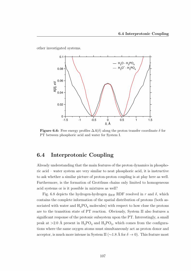
6.4 Interprotonic Coupling
other investigated systems.
-1.5 -1 -0.5 0 0.5 1 1.5δ, Å
0
0.02
0.04
0.06
0.08
0.1A
[δ],
eV
H2O - H3PO4
H3O+ - H3PO4
Figure 6.6: Free energy profiles ∆A(δ) along the proton transfer coordinate δ forPT between phosphoric acid and water for System I.
6.4 Interprotonic Coupling
Already understanding that the main features of the proton dynamics in phospho-
ric acid – water system are very similar to neat phosphoric acid, it is instructive
to ask whether a similar picture of proton-proton coupling is at play here as well.
Furthermore, is the formation of Grotthuss chains only limited to homogeneous
acid systems or is it possible in mixtures as well?
Fig. 6.8 depicts the hydrogen-hydrogen gHH RDF resolved in r and δ, which
contains the complete information of the spatial distribution of protons (both as-
sociated with water and H3PO4 molecules) with respect to how close the protons
are to the transition state of PT reaction. Obviously, System II also features a
significant response of the protonic subsystem upon the PT. Interestingly, a small
peak at >2.0 A present in H3PO4 and H3PO3, which comes from the configura-
tions where the same oxygen atoms must simultaneously act as proton donor and
acceptor, is much more intense in System II (∼1.8 A for δ → 0). This feature most
107

6. PHOSPHORIC ACID AND WATER MIXTURES
-1 0 1δ, Å
0
0.02
0.04
0.06
0.08
0.1
0.12
A[δ
], eV
All protonsH3PO4 - H3PO4
H4PO4+ - (H3PO4)n
H2PO4- - (H3PO4)n
H3PO4 - H2O
H2O - H2O
H3O+ - (H2O)n
H3O+ - (H3PO4)n
H4PO4+ - (H2O)n
Figure 6.7: Free energy profiles ∆A(δ) along the proton transfer coordinate δ forall protons and different proton donor/acceptor pairs in System II.
probably arises from a strong proton-proton coupling around the positive core of
the H3O+ ion. In general, the addition of water increases the H/O ratio and
overall proton concentration, leading to stronger electrostatic coupling between
the protons. Moreover, the main peak at ∼3.9 A also shows a marked increase
for δ → 0, in a similar fashion as the gHH(δ, r) of neat acid systems. Fig. 6.8
suggests that qualitatively very similar mechanism governing proton dynamics
and transport are at play in phosphoric acid – water mixtures as that previously
described for neat systems. The H-bonds in System II are on average very similar
in strength and hence highly polarizable. The PT events are obviously strongly
correlated to the dynamics of surrounding protonic subsystem opening a possibil-
ity for strong mutual protonic polarization and the build up of extended polarized
chains. In the next section, the question whether this behavior could also lead to
the formation of extended Grotthuss chains is addressed.
108

6.5 On the Formation of Grotthuss Chains and Proton TransportMechanism
1.0 2.0 3.0 4.0 5.0 6.0 7.00.0
0.2
0.4
0.6
0.8
1.0
1.2
1.4
1.6
0
0.2
0.4
0.6
0.8
1
1.2
1.4
1.6
1.8
2
r,
δ,
gHH
(r,δ)
Å
Å
δeq
~ 0.65 Å
Figure 6.8: gHH(SystemII) radial distribution function resolved in r and δ, con-taining information about the spatial distribution of protons with respect to δ (δeqis the equilibrium value in the simulation).
6.5 On the Formation of Grotthuss Chains and
Proton Transport Mechanism
In the first part of this chapter we established that the properties of H-bonding,
molecular vibrations and proton transfer in phosphoric acid – water mixtures,
even at 1:1 molar ratio, are surprisingly similar to those of pure phosphoric acid.
Moreover, there is a similarly strong correlation between the PT events and the
dynamics of surrounding protons. Can this coupling lead to chains of correlated
PTs, which in this case would involve not only phosphoric acid, but also water
molecules and would be terminated by H4PO+4 or H3O+ and H2PO−4 species. In
order to prove this hypothesis, we make use of the same proton coupling cor-
relation function, initially developed for phosphoric acid (Eq. 4.10 in Sec. 4.9).
In the calculation of the C(n), the phosphate tetrahedra and the water’s oxygen
109

6. PHOSPHORIC ACID AND WATER MIXTURES
atoms are treated as equivalent vertices in the graph-theoretical framework, used
in Eq. 4.10 (N = NPO4+ NOW
). The calculated C(n) for System II is presented
in Fig. 6.9 (C(n) for phosphoric acid (Fig. 4.16) is used for comparison). The
results indicate that the probability of two quasi-coherent PT events (τres = 0)
within two neighboring H-bonds in System II is ∼4%, which is about two times
lower than in neat H3PO4. Upon the increase of relay time parameter, allowing
for the relaxation of H-bond network around the displaced proton, the proba-
bilities of forming extended polarized chains start to increase. At τres = 50 fs,
the probabilities to form chains of three and four consecutive H-bonds are ∼18%
and ∼2%, respectively. Evidently, these values are significantly lower than in
the case of neat phosphoric acid (∼30% and ∼10%), indicating that the presence
of water tends to oppose the formation of Grotthuss chains. The representative
snapshots of the self-dissociation/neutralization and polarized chain formation
processes in System II showing this coupling, as extracted from the AIMD tra-
jectory, are presented in Fig. 6.10. The entire sequence features several intercon-
version events between various charged species, including H3O+ (both Zundel-
and Eigen-like forms), H4PO+4 and H2PO−4 . The sequence starts with one of the
water molecules already having an excess proton (Eigen-like) and one dihydrogen
phosphate species (Fig. 6.10 (a)). Then, one of the protons is transferred through
a Zundel-like state to another water molecule (Fig. 6.10 (b) and (c)). It is impor-
tant to note that both water molecules share one H-bond but, in principle, are
solvated by phosphate species (two are depicted), which in turn are bound by a
common H-bond. As previously shown, all H-bonds in this complex are of very
similar strength, therefore the mutual proton motion is strongly coupled and a
more distant proton can be further transferred to the phosphate (Fig. 6.10 (d)
and (e)). The latter process can be formally seen as a neutralization reaction
between two species carrying excess charges (H3O+ and H2PO−4 ). Furthermore,
the H-bond between the two water molecules is weakened and easily breaks, since
none of the molecules has an excess proton thus more resembling the H-bonds
in ‘normal’ liquid water. The breakage of this bond, allows the second water
molecule to easily reorient (Fig. 6.10 (e) and (f)) and start the solvent depolar-
ization process. This event certainly creates a new termination and shortens the
initial Grotthuss chain. Fig. 6.10 (f), (g) and (h) depict a formally new self-
110

6.5 On the Formation of Grotthuss Chains and Proton TransportMechanism
dissociative event between two H3PO4 molecules and a Grotthuss chain of three
H-bonds forming between three phosphate species and one water molecule.
0 1 2 3 4 5 6n (connectivity)
0
0.2
0.4
0.6
0.8
1
C (
n)
H3PO
4 - H
2O (1:1); τ
res = 0 fs
H3PO
4 - H
2O (1:1); τ
res = 50 fs
H3PO
4; τ
res = 50 fs
H3PO
4; τ
res = 0 fs
Figure 6.9: Proton coupling correlation function Cpc(n) as a function of connec-tivity n for pure H3PO4 and System II. δcut ≤ 0.1 A and τres = 0 and 50 fs.
Fig. 6.10 depicts some representative snapshots of the self-dissociation/neutra-
lization and polarized chain formation processes in System II. The entire sequence
features several interconversion events between various charged species, including
H3O+ (both Zundel- and Eigen-like forms), H4PO+4 and H2PO−4 . The sequence
is started with one of the water molecules having an excess proton and one dihy-
drogen phosphate (Fig. 6.10 (a)). Then one of the protons is transferred though
a Zundel-like state to another water molecule (Fig. 6.10 (b) and (c)). It is im-
portant to note that both water molecules share one H-bond, but are at the ends
solvated by two phosphate species, which in turn have a common H-bond. All
the H-bonds in this complex are of very similar strength, therefore the proton can
be further transferred to the phosphate due to the mutual interprotonic coupling
(Fig. 6.10 (d) and (e)). The latter process can be seen as a neutralization reaction
between two species carrying excess charge (H3O+ and H2PO−4 ). Moreover, the
H-bond joining two water molecules is weakened (none of the molecules have an
111

6. PHOSPHORIC ACID AND WATER MIXTURES
excess proton) and breaks, letting the second water molecule reorient (Fig. 6.10
(e) and (f)). This event creates a new termination of Grotthuss chain. (f), (g)
and (h) in Fig. 6.10 depict a self-dissociative event between two H3PO4 molecules
and a Grotthuss chain of three H-bond forming between three phosphate species
and one water molecule.
112

6.5 On the Formation of Grotthuss Chains and Proton TransportMechanism
a)-
b)
+
d)
+
-
a) -
+
c)c)-
+
-
+
e) f)-
+
g)-
+
h)
Figure 6.10: Snapshots of the elementary proton structural diffusion steps inSystem II. The charged ion pair is indicated with (+) and (-). The arrows denotethe proton hops and molecular reorientations.
113

6. PHOSPHORIC ACID AND WATER MIXTURES
114

7
Conclusions
Understanding proton transport in hydrogen bonded systems on the molecular
level remains a fundamental problem in many areas of science ranging from bio-
logical processes to electrochemical energy conversion. In this work, the molecular
details of proton transport mechanisms in a number of phosphorus oxoacid sys-
tems are addressed. Currently, the experimental probes able to resolve the time
and length scales of these mechanisms are still lacking. Therefore, molecular sim-
ulation techniques prove to be indispensable for the study of proton transport
processes. Proton transfer is essentially a chemical reaction, which requires a dy-
namical self-consistent description of bond breaking and forming at the quantum
mechanical level. In a large part thanks to ab initio molecular dynamics simu-
lations, water became the first and remains the only bulk H-bonded network for
which at least the mobility mechanism of protonic defects has been envisioned
in great detail. In this work, a number of systems showing the highest known
proton conductivities are studied. Five different systems based on phosphorus
oxoanions: phosphoric, phosphonic and phosphinic acids and phosphoric acid –
water mixtures are investigated with the help of ab initio molecular dynamics
simulations.
For the first time, the microscopic mechanism of proton conduction in phos-
phoric acid, the central compound of this study, is revealed. We find that the
high density of strong, polarizable H-bonds are involved in coupled proton motion
and a pronounced protic dielectric response of the H3PO4 medium, thus form-
ing extended, polarized (Grotthuss) chains up to six molecules, in the close sense
115

7. CONCLUSIONS
to the earlier notions of aqueous proton transport but never truly observed in
H-bonded systems. It is commonly understood that the presence of only short,
strong H-bonds would lead to protonic ordering and slow dynamics, preventing
rapid solvent reorientation (depolarization) processes and fast charge transport,
however, phosphoric acid has a very peculiar H-bond network topology: an im-
balance in the numbers of potential proton donor and acceptor sites (three OH
donors and only one non-protonated oxygen) is anticipated to lead to configura-
tional frustration and disorder. In the mechanism proposed in this work, it is the
interplay between these chains and a frustrated H-bond network, which is found
to lead to extremely high proton conductivity in phosphoric acid. This mecha-
nism is in stark contrast to that of water, which has negligible intrinsic proton
conductivity, but can transport the excess protonic charges at anomalously high
rates, occurring not through extended chains but rather through local H-bond
rearrangements that drive individual proton transfer reactions.
The next part of this work addresses an immediately arising question: why
does phosphonic acid, which has even stronger H-bonds but does not posses the
same frustrated hydrogen bond network as phosphoric acid (donor/ac-ceptor ratio
2:2), still shows good proton conductivity. The experimentally measured proton
structural diffusion in phosphonic acid constitutes ∼90% of the total conductiv-
ity, which is only slightly lower than that of H3PO4. Moreover, in phosphinic
acid, which has an even lower proton donor versus acceptor ratio (1:2), ∼20% of
the reasonably good proton conductivity comes from structural diffusion. The
presence of very strong H-bonds in H3PO3 and H3PO2 allow for a mutual proton-
proton coupling and formation of polarized H-bonded chains, however, on the
other hand, this process is counteracted by a much stronger hydrodynamic and
dipolar background existing in these systems. Therefore, the average length of
Grotthuss chains building up in phosphonic and phosphinic acid systems is sig-
nificantly shorter than in the case of phosphoric acid. Furthermore, the results
show that weak H-bond configurations, although not an property of the H-bond
network, are still forming in a dynamical sense due to liquid disorder, essentially
playing the same role in the solvent reorientation process as in H3PO4.
Nearly all types of chemical perturbations destroy the proton conducting prop-
erties of phosphoric acid, apart from the severe conductivity reduction caused by
116
the addition of bases, even the addition of acids leads to some decrease in conduc-
tivity. Apparently, the only dopant that increases the conductivity of H3PO4 is
water. The question of whether the excess water simply accelerates the intrinsic
proton conduction process already operating in H3PO4 or the entire proton con-
duction mechanism changes, has not been clear yet and was therefore, addressed
in the last chapter of this work. The results show than neither at the very low
nor at 50% mol. concentration, water acts as classical Brønsted base, abstracting
protons from phosphoric acid molecules and only contributing to the proton con-
ductivity through the vehicular diffusion of H3O+ species. From the comparison
of the simulated proton diffusion coefficients in 1:1 H3PO4 − H2O system, the
contribution due to structural diffusion is as high as 70%. Moreover, the H-bond
structure and vibrational properties of this system are virtually identical to those
of neat phosphoric acid and unlike those of water. This leads to similarly strong
proton-proton interaction and mutual protonic polarizability and the formation
of extended Grotthuss chains of up to three H-bonds. Although the dielectric and
hydrodynamic properties of water in these systems are significantly reduced, it
still increases the electrostatic penalty for the formation of polarized chains. On
the other hand, the nature of water increases the configurational entropy of the
system, providing new possibilities for efficient solvent reorganization, which, in
addition to the vehicular contribution to the proton transport lead to very high
proton conductivities.
The understanding of the molecular details of proton transport in phospho-
rus oxoacid systems has relevance for many fields of science such as chemistry,
engineering and biophysics. Our findings show the limits of proton transport
at the fundamental level – strong hydrogen bonding does not necessarily lead
to protonic ordering and slow dynamics. The proposed mechanisms show how
weak solvent coupling and sufficient degree of configurational disorder can lead
to fast proton transport. These systems can be regarded as a prototype models
for understanding molecular proton transport mechanisms in many other proton
conductors. This could serve as the first step in overcoming many technical hur-
dles concerning the use of phosphate based materials as electrolytes in e.g. fuel
cells. Moreover, the abundance and crucial role of phosphates in the chemistry
of life are relevant in the light of our findings. The recent view of chemiosmotic
117

7. CONCLUSIONS
theory of ATP synthesis suggest that the protons building up the gradient are
transported near the surface region of the phospholipid membrane rather than
quickly equilibrating with the bulk aqueous phase. Although, the active role of the
phospholipid membrane for the proton transport has been firmly established, a
complete molecular scale understanding of this process has not yet been achieved.
The molecular understanding of proton transport mechanism in neat phosphorus
oxoacids could serve as the next step towards the further elucidation of one of the
most important biological processes occurring at the phosphate/water interface.
118

References
[1] K. D. Kreuer. Chem. Mat., 8, 610–641, 1996.
[2] K. D. Kreuer, S. J. Paddison, E. Spohr and M. Schuster. Chem. Rev., 104, 4637–4678, 2004.
[3] D. Marx. ChemPhysChem, 7(9), 1848–1870, 2006.
[4] T. E. DeCoursey. Physiol. Rev., 83, 475–579, 2003.
[5] C. A. Wraight. Biochim. Biophys. Acta., 1757(8), 886–912, 2006.
[6] K. D. Kreuer. Solid State Ionics, 136, 149–160, 2000.
[7] N. Agmon. Chem. Phys. Lett., 244, 456–462, 1995.
[8] N. Agmon. Chem. Phys. Lett., 319(3-4), 247–252, 2000.
[9] M. E. Tuckerman, D. Marx, M. L. Klein and M. Parrinello. Science, 275(5301), 817–820, 1997.
[10] D. Marx, M. E. Tuckerman, J. Hutter and M. Parrinello. Nature, 397(6720), 601–604, 1999.
[11] M. E. Tuckerman, D. Marx and M. Parrinello. Nature, 417(6892), 925–929, 2002.
[12] R. Vuilleumier and D. Borgis. J. Phys. Chem. B, 102(22), 4261–4264, 1998.
[13] R. Vuilleumier and D. Borgis. J. Chem. Phys., 111(9), 4251–4266, 1999.
[14] U. W. Schmitt and G. A. Voth. J. Chem. Phys., 111(20), 9361–9381, 1999.
[15] J. Lobaugh and G. A. Voth. J. Chem. Phys., 104(5), 2056–2069, 1996.
[16] T. J. F. Day, U. W. Schmitt and G. A. Voth. J. Am. Chem. Soc., 122(48), 12027–12028, 2000.
[17] O. Markovitch, H. Chen, S. Izvekov, F. Paesani, G. A. Voth and N. Agmon. J. Phys. Chem. B, 112(31),9456–9466, 2008.
[18] T. C. Berkelbach, H.-S. Lee and M. E. Tuckerman. Phys. Rev. Lett., 103(23), 238302, 2009.
[19] D. Marx, A. Chandra and M. E. Tuckerman. Chem. Rev., 110(4), 2174–2216, 2010.
[20] A. Botti, F. Bruni, S. Imberti, M. A. Ricci and A. K. Soper. J. Chem. Phys., 119(10), 5001–5004, 2003.
[21] S. Woutersen and H. J. Bakker. Phys. Rev. Lett., 96(13), 138305, 2006.
[22] C. D. Cappa, J. D. Smith, B. M. Messer, R. C. Cohen and R. J. Saykally. J. Phys. Chem. A, 111(22),4776–4785, 2007.
[23] E. F. Aziz, N. Ottosson, M. Faubel, I. V. Hertel and B. Winter. Nature, 455(7209), 89–91, 2008.
119

REFERENCES
[24] K. J. Tielrooij, R. L. A. Timmer, H. J. Bakker and M. Bonn. Phys. Rev. Lett., 102(19), 198303, 2009.
[25] S. T. Roberts, P. B. Petersen, K. Ramashesha, A. Tokmakoff, I. S. Ufimtsev and T. J. Martinez. Proc.Natl. Acad. Sci., 106(36), 15154–15159, 2009.
[26] K. D. Kreuer. J. Membr. Sci., 185, 29–39, 2001.
[27] K. Mauritz and R. Moore. Chem. Rev., 104(10), 4535–4585, 2004.
[28] S. Paddison. Ann. Rev. Mater. Res., 33, 289–319, 2003.
[29] J. Wainright, J. Wang, D. Weng, R. Savinell and M. Litt. J. Electrochem. Soc., 142(7), L121–L123, 1995.
[30] M. Schuster and W. Meyer. Annu. Rev. Mater. Res., 33, 233–261, 2003.
[31] Y. Ma, J. Wainright, M. Litt and R. Savinell. J. Electrochem. Soc., 151(1), A8–A16, 2004.
[32] H. Steininger, M. Schuster, K. D. Kreuer, A. Kaltbeitzel, B. Bingoel, W. H. Meyer, S. Schauff, G. Brun-klaus, J. Maier and H. W. Spiess. Phys. Chem. Chem. Phys., 9(15), 1764–1773, 2007.
[33] M. B. Herath, S. E. Creager, A. Kitaygorodskiy and D. D. DesMarteau. ChemPhysChem, 11(13), 2871–2878, 2010.
[34] F. H. Westheimer. Science, 235(4793), 1173–1178, 1987.
[35] K. D. Kreuer, A. Rabenau and W. Weppner. Angew. Chem. Int. Ed., 21(3), 208–209, 1982.
[36] C. J. T. de Grotthuss. Ann. Chim. (Paris), LVIII, 54–74, 1806.
[37] J. N. Collie and T. Tickle. J. Chem. Soc., 75, 710, 1899.
[38] C. Dempwolff. Phys. Z., 5, 637, 1904.
[39] S. Tijmstra. Z. Elektrochem., 11, 249, 1905.
[40] H. Danneel. Z. Elektrochem., 11, 249, 1905.
[41] E. Huckel. Z. Elektrochem., 34, 546, 1928.
[42] J. D. Bernal and R. H. Fowler. J. Chem. Phys., 1(8), 515–548, 1933.
[43] G. Wannier. Ann. Phys. (Leipzig), 24(6), 545–568, 1935.
[44] A. Gierer. Z. Naturforsch., 5a, 581, 1950.
[45] B. E. Conway, J. O. Bockris and H. Linton. J. Chem. Phys., 24(4), 834–850, 1956.
[46] M. Eigen and L. D. Mayer. Proc. R. Soc. Lon. Ser. A, 247(1251), 505–533, 1958.
[47] G. Halle, B.; Karlstrom. J. Chem. Soc. Far. Trans., 79, 1047, 1983.
[48] H. G. Hertz, B. M. Braun, K. J. Muller and R. Maurer. J. Chem. Educ, 64(9), 777–784, 1987.
[49] M. E. Tuckerman, K. Laasonen, M. Sprik and M. Parrinello. J. Phys.-Cond. Mat., 6, A93–A100, 1994.
[50] M. E. Tuckerman, K. Laasonen, M. Sprik and M. Parrinello. J. Phys. Chem., 99(16), 5749–5752, 1995.
[51] M. E. Tuckerman, K. Laasonen, M. Sprik and M. Parrinello. J. Chem. Phys., 103(1), 150–161, 1995.
[52] S. Izvekov and G. A. Voth. J. Chem. Phys., 123, 044505, 2005.
120

REFERENCES
[53] A. Chandra, M. E. Tuckerman and D. Marx. Phys. Rev. Lett., 99(14), 145901, 2007.
[54] E. T. J. Nibbering and T. Elsaesser. Chem. Rev., 104(4), 1887–1914, 2004.
[55] H. J. Bakker and J. L. Skinner. Chem. Rev., 110(3), 1498–1517, 2010.
[56] R. A. Marcus. J. Chem. Phys., 24(5), 966–978, 1956.
[57] R. A. Marcus. Rev. Mod. Phys., 65(3), 599–610, 1993.
[58] N. Agmon. Isr. J. Chem., 39(3-4), 493–502, 1999.
[59] G. Zundel. Adv. Chem. Phys., 111, 1, 2000.
[60] T. Dippel and K. D. Kreuer. Solid State Ionics, 46(1-2), 3–9, 1991.
[61] C. Dellago, M. Naor and G. Hummer. Phys. Rev. Lett., 90(10), 105902, 2003.
[62] C. Dellago and G. Hummer. Phys. Rev. Lett., 97(24), 245901, 2006.
[63] Z. Cao, Y. Peng, T. Yan, S. Li, A. Li and G. A. Voth. J. Am. Chem. Soc., 132(33), 11395–11397, 2010.
[64] R. Pomes and B. Roux. Biophys. J., 82(5), 2304–2316, 2002.
[65] M. Schuster, K.-D. Kreuer, H. Steininger and J. Maier. Solid State Ionics, 179(15-16), 523–528, 2008.
[66] L. Vilciauskas, C. C. de Araujo and K. D. Kreuer. Solid State Ionics, (accepted), 2012.
[67] R. A. Munson. J. Phys. Chem., 68, 3374–3377, 1964.
[68] T. Dippel, K. D. Kreuer, J. C. Lassegues and D. Rodriguez. Solid State Ionics, 61(1-3), 41–46, 1993.
[69] D. Chin and H. Chang. J. Appl. Electrochem., 19, 95–99, 1989.
[70] R. H. Blessing. Acta Cryst. B, 44, 334–340, 1988.
[71] G. Becker, H. D. Hausen, O. Mundt, W. Schwarz, C. T. Wagner and T. Vogt. Z. Anorg. Allg. Chem.,591(12), 17–31, 1990.
[72] J. M. Williams and S. W. Peterson. Spectrosc. Inorg. Chem., 2, 1–56, 1971.
[73] E. Tsuchida. J. Phys. Soc. Japan, 75(5), 054801, 2006.
[74] L. Vilciauskas, S. J. Paddison and K. D. Kreuer. J. Phys. Chem. A, 113(32), 9193–9201, 2009.
[75] N. Greenwood and A. Thompson. Proc. Chem. Soc., (12), 352–353, 1958.
[76] N. N. Greenwood and A. Thompson. J. Chem. Soc., 3485–3492, 1959.
[77] N. Greenwood and A. Thompson. J. Chem. Soc., 3864–3867, 1959.
[78] R. A. Munson and M. E. Lazarus. J. Phys. Chem., 71(10), 3245–3248, 1967.
[79] Y. Aihara, A. Sonai, M. Hattori and K. Hayamizu. J. Phys. Chem. B, 110, 24999–25006, 2006.
[80] T. Dippel, N. G. Hainovsky, K. D. Kreuer, W. Munch and J. Maier. Ferroelectrics, 167, 59, 1995.
[81] R. Janoschek, E. G. Weidemann, G. Zundel and H. Pfeiffer. J. Am. Chem. Soc., 94(7), 2387–2396, 1972.
[82] M. Leuchs and G. Zundel. Can. J. Chem., 57(5), 487–493, 1979.
121

REFERENCES
[83] A. Schechter and R. Savinell. Solid State Ionics, 147(1-2), 181–187, 2002.
[84] R. A. Munson. J. Phys. Chem., 69, 1761–1762, 1965.
[85] W. Munch, K. D. Kreuer, W. Silvestri, J. Maier and G. Seifert. Solid State Ionics, 145(1-4), 437–443,2001.
[86] M. Iannuzzi and M. Parrinello. Phys. Rev. Lett., 93(2), 025901, 2004.
[87] M. Iannuzzi. J. Chem. Phys., 124(20), 204710, 2006.
[88] H. Hen, T. Yan and G. A. Voth. J. Phys. Chem. A, 113(16), 4507–4517, 2009.
[89] F. Shimojo, K. Hoshino and H. Okazaki. Solid State Ionics, 113, 319–323, 1998.
[90] F. Shimojo and K. Hoshino. Solid State Ionics, 145(1-4), 421–427, 2001.
[91] W. Munch, K. D. Kreuer, G. Seifert and J. Maier. Solid State Ionics, 136, 183–189, 2000.
[92] K. Kreuer. Ann. Rev. Mater. Res., 33, 333–359, 2003.
[93] Q. Zhang, G. Wahnstrom, M. Bjorketun, S. Gao and E. Wang. Phys. Rev. Lett., 101(21), 215902, 2008.
[94] B. Frick and et al. to be published.
[95] Y. Iwadate, Y. Tani, K. Fukushima, M. Misawa, T. Fukunaga, K. Itoh and T. Nakazawa. J. Neutron.Res., 13(1), 139–144, 2005.
[96] J.-O. Joswig and G. Seifert. J. Phys. Chem. B, 113(25), 8475–8480, 2009.
[97] C. M. Maupin, B. Aradi and G. A. Voth. Journal Of Physical Chemistry B, 114(20), 6922–6931, 2010.
[98] S. Detoni, D. Hadzi and B. Orel. J. Mol. Struc., 33, 279–288, 1976.
[99] M. A. Vargas, R. A. Vargas and B. E. Mellander. Electrochim. Acta, 44(24), 4227–4232, 1999.
[100] M. A. Vargas, R. A. Vargas and B. E. Mellander. Electrochim. Acta, 45(8-9), 1399–1403, 2000.
[101] M. A. Vargas, R. A. Vargas and B. E. Mellander. Phys. Stat. Sol. B, 220(1), 615–624, 2000.
[102] R. Vargas, V. Zapata, E. Matallana and M. Vargas. Electrochim. Acta, 46(10-11), 1699–1702, 2001.
[103] N. Sammes, R. Bove and K. Stahl. Curr. Opin. Solid. St. Mat. Sci., 8(5), 372–378, 2004.
[104] A. Bozkurt, M. Ise, K. D. Kreuer, W. H. Meyer and G. Wegner. Solid State Ionics, 125(1-4), 225–233,1999.
[105] M. Schuster, T. Rager, A. Noda, K. D. Kreuer and J. Maier. Fuel Cells, 5, 355–365, 2005.
[106] H. Steininger, M. Schuster, K. D. Kreuer and J. Maier. Solid State Ionics, 177(26-32), 2457–2462, 2006.
[107] J. P. Lassegues. in P. Colomban Proton Conductors: Solids, membranes and gelss - materials and devices,311–326. Cambridge University Press, 1992.
[108] Q. Li, J. O. Jensen, R. F. Savinell and N. J. Bjerrum. Prog. Polym. Sci., 34(5), 449–477, 2009.
[109] A. Kaltbeitzel, S. Schauff, H. Steininger, B. Bingoel, G. Brunklaus, W. H. Meyer and H. W. Spiess. SolidState Ionics, 178(7-10), 469–474, 2007.
[110] A. Warshel and R. M. Weiss. J. Am. Chem. Soc., 102, 6218, 1980.
122

REFERENCES
[111] A. C. T. van Duin, S. Dasgupta, F. Lorant and W. A. Goddard. J. Phys. Chem. A, 105(41), 9396–9409,2001.
[112] U. W. Schmitt and G. A. Voth. J. Phys. Chem. B, 102(29), 5547–5551, 1998.
[113] Y. Wu, H. Chen, F. Wang, F. Paesani and G. A. Voth. J. Phys. Chem. B, 112(2), 467–482, 2008.
[114] H. Chen, G. A. Voth and N. Agmon. J. Phys. Chem. B, 114(1), 333–339, 2010.
[115] D. Marx and J. Hutter. Ab Initio Molecular Dynamics: Basic Theory and Advanced Methods. CambridgeUniversity Press, New York, 2009.
[116] P. Hohenberg and W. Kohn. Phys. Rev., 136(3B), B864, 1964.
[117] W. Kohn and L. Sham. Phys. Rev., 140(4A), 1133, 1965.
[118] R. Car and M. Parrinello. Phys. Rev. Lett., 55(22), 2471–2474, 1985.
[119] J. Morrone and M. Tuckerman. J. Chem. Phys., 117(9), 4403–4413, 2002.
[120] J. Morrone, K. Hasllinger and M. Tuckerman. J. Phys. Chem. B, 110(8), 3712–3720, 2006.
[121] M. Diraison, G. J. Martyna and M. E. Tuckerman. J. Chem. Phys., 111(3), 1096–1103, 1999.
[122] Y. Liu and M. Tuckerman. J. Phys. Chem. B, 105(28), 6598–6610, 2001.
[123] U. Rothlisberger and M. Parrinello. J. Chem. Phys., 106(11), 4658–4664, 1997.
[124] S. Raugei and M. L. Klein. ChemPhysChem, 5(10), 1569–1576, 2004.
[125] B. C. Wood and N. Marzari. Phys. Rev. B, 76(13), 134301, 2007.
[126] H.-S. Lee and M. E. Tuckerman. J. Phys. Chem. C, 112(26), 9917–9930, 2008.
[127] R. M. Martin. Electronic Structure: Basic Theory and Practical Methods. Cambridge University Press,Cambridge, 2004.
[128] J. Kohanoff. Electronic Structure Calculations for Solids and Molecules: Theory and ComputationalMethods. Cambridge University Press, New York, 2006.
[129] R. G. Parr and W. Yang. Density-Functional Theory of Atoms and Molecules. Oxford University Press,New York, 1994.
[130] W. Koch and M. C. Holthausen. A Chemist’s Guide to Density Functional Theory. Wiley-VCH, Wein-heim, 2001.
[131] R. M. Dreizler and E. K. U. Gross. Density Functional Theory: An Approach to the Quantum Many-BodyProblem. Springer-Verlag, 1991.
[132] A. D. Becke. J. Chem. Phys., 98, 1372–1377, 1993.
[133] A. D. Becke. J. Chem. Phys., 98, 5648–5652, 1993.
[134] T. Todorova, A. P. Seitsonen, J. Hutter, I. F. W. Kuo and C. J. Mundy. J. Phys. Chem. B, 110(8),3685–3691, 2006.
[135] M. Guidon, F. Schiffmann, J. Hutter and J. VandeVondele. J. Chem. Phys., 128(21), 214104, 2008.
[136] C. Zhang, D. Donadio, F. Gygi and G. Galli. J. Chem. Theory. Comput., 7(5), 1443–1449, 2011.
[137] J. M. Tao, J. P. Perdew, V. N. Staroverov and G. E. Scuseria. Phys. Rev. Lett., 91(14), 146401, 2003.
123

REFERENCES
[138] G. Lippert, J. Hutter and M. Parrinello. Mol. Phys., 92(3), 477–487, 1997.
[139] G. Lippert, J. Hutter and M. Parrinello. Theor. Chem. Acc., 103(2), 124–140, 1999.
[140] J. VandeVondele, M. Krack, F. Mohamed, M. Parrinello, T. Chassaing and J. Hutter. Comp. Phys.Comm., 167(2), 103–128, 2005.
[141] D. R. Hamann, M. Schluter and C. Chiang. Phys. Rev. Lett., 43, 1494–1497, 1979.
[142] S. Goedecker, M. Teter and J. Hutter. Phys. Rev. B, 54(3), 1703–1710, 1996.
[143] G. Martyna, M. Klein and M. Tuckerman. J. Chem. Phys., 97(4), 2635–2643, 1992.
[144] M. E. Tuckerman, B. J. Berne, G. J. Martyna and M. L. Klein. J. Chem. Phys., 99, 2796, 1993.
[145] M. E. Tuckerman. Statistical Mechanics: Theory and Molecular Simulation. Oxford University Press,New York, 2010.
[146] Max-Planck-Institut fur Festkorperforschung, Stuttgart and IBM Zurich Research Laboratory. CPMD;ver. 3.13, 1995-2010.
[147] A. D. Becke. Phys. Rev. A, 38, 3098, 1988.
[148] C. Lee, W. Yang and R. Parr. Phys. Rev. B, 37(2), 785–789, 1988.
[149] N. Troullier and J. Martins. Phys. Rev. B, 43(3), 1993–2006, 1991.
[150] The cp2k developers group.
[151] J. VandeVondele and J. Hutter. J. Chem. Phys., 127(11), 114105, 2007.
[152] J. Perdew, K. Burke and M. Ernzerhof. Phys. Rev. Lett., 77(18), 3865–3868, 1996.
[153] M. Krack. Theor. Chem. Acc., 114, 145–152, 2005.
[154] S. A. H. Spieser, B. R. Leeflang, L. M. J. Kroon-Batenburg and J. Kroon. J. Phys. Chem. A, 104(31),7333–7338, 2000.
[155] W. Humphrey, A. Dalke and K. Schulten. J. Mol. Graph., 14, 33–38, 1996.
[156] R. Tromp, S. Spieser and G. Neilson. J. Chem. Phys., 110(4), 2145–2150, 1999.
[157] B. Dunweg and K. Kremer. J. Chem. Phys., 99(9), 6983–6997, 1993.
[158] I. Yeh and G. Hummer. J. Phys. Chem. B, 108(40), 15873–15879, 2004.
[159] D. Laage and J. T. Hynes. J. Phys. Chem. B, 112(45), 14230–42, 2008.
[160] I. M. Svishchev and P. G. Kusalik. J. Phys. Chem., 98, 728–733, 1994.
[161] D. Laage and J. Hynes. Science, 311(5762), 832–835, 2006.
[162] F. H. Stillinger. Adv. Chem. Phys., 31, 1–101, 1975.
[163] D. C. Rapaport. Mol. Phys., 50, 1151, 1983.
[164] A. Luzar and D. Chandler. Nature, 379(6560), 55–57, 1996.
[165] A. Luzar. J. Chem. Phys., 113(23), 10663–10675, 2000.
[166] M. E. Tuckerman, A. Chandra and D. Marx. J. Chem. Phys., 133(12), 124108, 2010.
124

REFERENCES
[167] D. Marx, M. Tuckerman, J. Hutter and M. Parrinello. J. Phys.-Cond. Matt., 12, A153, 2000.
[168] L. Pauling. J. Am. Chem. Soc., 69(3), 542–553, 1947.
[169] N. Agmon. J. Mol. Liq., 73-4, 513–520, 1997.
[170] H. Lapid, N. Agmon, M. Petersen and G. Voth. J. Chem. Phys., 122, 014506, 2005.
[171] L. Vilciauskas, M. E. Tuckerman, G. Bester, S. J. Paddison and K. D. Kreuer. Nature Chemistry,(accepted), 2012.
[172] R. L. Hayes, S. J. Paddison and M. E. Tuckerman. J. Phys. Chem. B, 113(52), 16574–16589, 2009.
[173] P. Silvestrelli and M. Parrinello. Phys. Rev. Lett., 82(16), 3308–3311, 1999.
[174] M. Sharma, R. Resta and R. Car. Phys. Rev. Lett., 98(24), 247401, 2007.
[175] R. A. Munson. J. Chem. Phys., 40, 2044, 1964.
[176] R. Buchner, J. Barthel and J. Stauber. Chem. Phys. Lett., 306(1-2), 57–63, 1999.
[177] P. Geissler, C. Dellago, D. Chandler, J. Hutter and M. Parrinello. Science, 291(5511), 2121–2124, 2001.
[178] W. A. Jenkins and R. T. Jones. J. Am. Chem. Soc., 74(5), 1353–1354, 1952.
[179] M. Spaeth, K. D. Kreuer, J. Maier and C. Cramer. J. Sol. State Chem., 148(1), 169–177, 1999.
[180] A. C. Chapman and L. E. Thirlwell. Spectrochim. Acta, 20(6), 937–947, 1964.
[181] A. Simon, F. Feher and G. Schulze. Zeit. Anorg. Allg. Chem., 230(3), 289–307, 1937.
[182] P. M. Kiefer and J. T. Hynes. J. Phys. Chem. A, 106(9), 1834–1849, 2002.
[183] P. M. Kiefer and J. T. Hynes. J. Phys. Chem. A, 106(9), 1850–1861, 2002.
[184] E. Tang, D. D. Tommaso and N. H. de Leeuw. J. Chem. Phys., 130(23), 234502, 2009.
[185] A. Smondyrev and G. Voth. Biophys. J., 82(3), 1460–1468, 2002.
[186] H. L. Tepper and G. A. Voth. Biophys. J., 88(5), 3095–3108, 2005.
[187] H. L. Tepper and G. A. Voth. J. Phys. Chem. B, 110(42), 21327–21337, 2006.
[188] T. Yamashita and G. A. Voth. J. Phys. Chem. B, 114(1), 592–603, 2010.
[189] Y. Kameda, K. Sugawara, T. Hosaka, T. Usuki and O. Uemura. Bull. Chem. Soc. Japan, 73(5), 1105–1112, 2000.
[190] S. Chung, S. Bajue and S. Greenbaum. J. Chem. Phys., 112(19), 8515–8521, 2000.
125

REFERENCES
126

Lebenslauf
Linas Vilciauskas
NATIONALITAT: Litauisch
28. April 1983 geboren in Joniskis, Litauen.
BILDUNG:
Januar 2008 – Doktorarbeit zum Thema Mechanismen des Protonentransports inDezember 2011 Phosphorsaure und verwandten Systemen von Phosphor Oxosauren:
eine “ab initio” molekulardynamische Untersuchungam Max-Planck-Institut fur Festkorperforschung, Stuttgart.
April 2007 – Masterarbeit am Max-Planck-Institut fur FestkorperforschungOktober 2007 (Betreuer: Dr. K.-D. Kreuer) und an der Universitat Alabama
in Huntsville, USA (Betreuer: Prof. S. J. Paddison).
Oktober 2005 – Masterstudium der Werkstoffwissenschaft (Nanomaterialien)April 2007 an der Universitat Ulm, Deutschland.
Januar 2005 – Austauschsemester an der Universitat Lettland, Riga.Mai 2005
September 2001 – Bachelorstudium der Chemie an der Universitat Vilnius, Litauen.Juli 2005
September 1994 – Matas-Slanciauskas-Gymnasium Joniskis, Litauen.Juli 2001 Abiturabschluss mit Auszeichnung
September 1989 – Mittelschule Nr. 2, Joniskis, Litauen.Juni 1994
AUSZEICHNUNGEN
2005 – 2007 Stipendium des Deutschen akademischen Austauschdienstes(DAAD) fur Mastertudium an der Universitat Ulm.
2004 Stipendium der Litauischen Stiftung fur Wissenschaft und Studium.