prospects for open heavy flavor measurements via dimuons

HAL Id: dumas-01228767https://dumas.ccsd.cnrs.fr/dumas-01228767

Submitted on 9 Dec 2015

HAL is a multi-disciplinary open accessarchive for the deposit and dissemination of sci-entific research documents, whether they are pub-lished or not. The documents may come fromteaching and research institutions in France orabroad, or from public or private research centers.

L’archive ouverte pluridisciplinaire HAL, estdestinée au dépôt et à la diffusion de documentsscientifiques de niveau recherche, publiés ou non,émanant des établissements d’enseignement et derecherche français ou étrangers, des laboratoirespublics ou privés.

Distributed under a Creative Commons Attribution - NonCommercial - NoDerivatives| 4.0International License

Prospects for open heavy flavor measurements viadimuons in Pb-Pb collisions at √ s N N = 5.5 TeV with

the ALICE Muon Forward TrackerSamir Assouabi

To cite this version:Samir Assouabi. Prospects for open heavy flavor measurements via dimuons in Pb-Pb collisions at√ s N N = 5.5 TeV with the ALICE Muon Forward Tracker. High Energy Physics - Phenomenology[hep-ph]. 2015. �dumas-01228767�

https://dumas.ccsd.cnrs.fr/dumas-01228767

http://creativecommons.org/licenses/by-nc-nd/4.0/



https://hal.archives-ouvertes.fr

Master Sciences de la matiere

Deuxieme annee

Specialite : Physique des Particules

Rapport de stage

Juin 2015

Laboratoire de Physique Corpusculaire

Universite Blaise Pascal

Prospects for open heavy flavormeasurements via dimuons in Pb-Pbcollisions at

√sNN = 5.5 TeV with the

ALICE Muon Forward Tracker

Samir ASSOUABI

Responsable de stage : Lizardo VALENCIA PALOMO

Acknowledgments

First, I’d like to thank Lizardo for his continuous and tireless efforts, making this intership truelysatisfactory. I am glad to have accomplished this task with him, and definitely think that it was fruitful.It has been a little bit more than four months, and I am rejoiced to see the result.

I’d also like to thank the whole laboratory and its personnel, for having provided the conditions toperform this intership in a convenient fashion.

Contents

1 Introduction 4

2 Physics motivation 5

2.1 Heavy ion collisions and Quark Gluon Plasma (QGP) . . . . . . . . . . . . . . . . . . . . 5

2.1.1 The Standard Model . . . . . . . . . . . . . . . . . . . . . . . . . . . . . . . . . . 5

2.1.2 Quantum Chromodynamics (QCD) . . . . . . . . . . . . . . . . . . . . . . . . . . 5

2.1.3 The Quark Gluon Plasma . . . . . . . . . . . . . . . . . . . . . . . . . . . . . . . 6

2.1.4 Heavy ion collisions . . . . . . . . . . . . . . . . . . . . . . . . . . . . . . . . . . . 7

2.2 Open heavy flavors and their interests in the QGP study . . . . . . . . . . . . . . . . . . 7

2.2.1 Open Heavy Flavors . . . . . . . . . . . . . . . . . . . . . . . . . . . . . . . . . . 7

2.2.2 Nuclear modification factor . . . . . . . . . . . . . . . . . . . . . . . . . . . . . . 8

2.3 Some useful definitions . . . . . . . . . . . . . . . . . . . . . . . . . . . . . . . . . . . . . 9

3 The ALICE experiment 10

3.1 The Large Hadron Collider . . . . . . . . . . . . . . . . . . . . . . . . . . . . . . . . . . . 10

3.2 The ALICE experiment . . . . . . . . . . . . . . . . . . . . . . . . . . . . . . . . . . . . . 11

3.2.1 The upgrade of the ITS . . . . . . . . . . . . . . . . . . . . . . . . . . . . . . . . 11

3.2.2 The muon spectrometer . . . . . . . . . . . . . . . . . . . . . . . . . . . . . . . . 12

3.3 The Muon Forward Tracker (MFT) . . . . . . . . . . . . . . . . . . . . . . . . . . . . . . 13

3.3.1 The MFT working principle . . . . . . . . . . . . . . . . . . . . . . . . . . . . . . 13

3.3.2 New measurements . . . . . . . . . . . . . . . . . . . . . . . . . . . . . . . . . . . 15

4 Dimuons from open heavy flavors with the MFT 16

4.1 Definitions . . . . . . . . . . . . . . . . . . . . . . . . . . . . . . . . . . . . . . . . . . . . 16

4.1.1 Offset and weighted offset . . . . . . . . . . . . . . . . . . . . . . . . . . . . . . . 16

4.1.2 Signal, background, invariant mass regions and dimuon pT ranges . . . . . . . . . 16

4.2 Selection criteria . . . . . . . . . . . . . . . . . . . . . . . . . . . . . . . . . . . . . . . . 17

4.2.1 Single muon and dimuon cuts . . . . . . . . . . . . . . . . . . . . . . . . . . . . . 17

4.2.2 Impact of the cuts . . . . . . . . . . . . . . . . . . . . . . . . . . . . . . . . . . . 18

4.3 Reference charm, beauty and background templates . . . . . . . . . . . . . . . . . . . . . 19

4.4 Uncertainties estimation . . . . . . . . . . . . . . . . . . . . . . . . . . . . . . . . . . . . 22

4.4.1 Systematic uncertainties . . . . . . . . . . . . . . . . . . . . . . . . . . . . . . . . 22

4.4.2 Statistical errors . . . . . . . . . . . . . . . . . . . . . . . . . . . . . . . . . . . . 26

5 Results 27

5.1 Statistical errors and systematic uncertainties . . . . . . . . . . . . . . . . . . . . . . . . 27

5.2 Discussion . . . . . . . . . . . . . . . . . . . . . . . . . . . . . . . . . . . . . . . . . . . . 29

6 Conclusions and outlook 30

A Appendix 32

3

1 Introduction

The ALICE (A Large Ion Collider Experiment) experiment is one the four main experiments at theLHC (Large Hadron Collider). ALICE was designed to study high energy heavy ion collisions. Thesecollisions fulfill the requirements to recreate a state of matter where quarks and gluons, usually confinedinside structures called “hadrons”, become deconfined. This state of matter is known as the QuarkGluon Plasma (QGP), and the Universe, one microsecond after the Big Bang, was in a QGP state.

Due to the extremely short life-time of the QGP, a direct observation of the plasma is not possible.Among the possible probes of the QGP, heavy quarks are of particular interest because they are producedin the hard-scattering processes and experience the whole evolution of the system.

As it is the case for many LHC experiments, ALICE will be upgraded over the years. One of theALICE upgrades scheduled for the run III of the LHC (that will start in 2019) is the Muon ForwardTracker (MFT). The MFT will be used in conjunction with the muon spectrometer at forward rapiditiesand the upgraded Inner Tracking System detectors, in the central barrel. A current muon spectrometer’ssetup limitation is the impossibility to distinguish beauty and charm hadrons through their semimuonicdecays. The MFT is expected to address this by allowing such distinction.

In order to separate the open charm and open beauty, there exists an observable, called the offset,that can be used. Due to the different mean lifetimes of the beauty and charm hadrons, their offsetdistributions would be significantly different. Separating the muons coming from open charm and openbeauty will give us more insight on the QGP.

In this study, we’ll evaluate the future MFT perfomances in Pb-Pb collisions for the open charmand open beauty measurements, using the offset distributions, via dimuons. For this, we’ll start bydefining the theoretical and experimental frameworks. Then we’ll use a Monte-Carlo simulation of Pb-Pb collisions, generated with the expected conditions of run III, to evaluate the uncertainties for theopen beauty and open charm extraction with the MFT.

4

2 Physics motivation

This first part will introduce the physics of this internship, begining by the theoretical background (theStandard Model) with a brief description of its main concepts, followed by a closer look at the physicsmotivations that are pursued through this study, first by introducing the particles studied (open heavyflavors), and then by explaining the interests in their study.

2.1 Heavy ion collisions and Quark Gluon Plasma (QGP)

2.1.1 The Standard Model

The Standard Model is the theory that describes the elementary particles and their interactions[1].Among the fundamental particles, there are six quarks (q) that are grouped in three families:(

updown

) (charmstrange

) (top

beauty

)Quark composed particles are called hadrons. Hadrons are in turn divided into two groups: baryons

made of three quarks (qq′q′′), and mesons made of a quark and an antiquark (qq′). Where q, q′, q′ and q′′

are any of the previously mentionned quarks, except the top quark that decays before it can hadronizedue to its very large mass (∼ 173 GeV/c2)[2].

The Standard Model describes three fundamental interactions: electromagnetic, weak and strong.For each interaction, there are gauge bosons associated to it that act like “force carriers”: the elec-tromagnetic interaction has one gauge boson called the photon (γ); the weak interactions has threemassive gauge bosons named W+, W− and Z0; and the strong interaction has eight massless bosonscalled gluons (g). In addition to that, the Standar Model features another bosonic particle which is nota gauge boson: the Higgs boson. It is responsible for the masses of the other particles.

In this study we’ll focus on particles that have either a charm (c) or beauty (b) quark in its com-position, called open heavy flavor (D and B hadrons, respectively) because of the significant masses ofthese two quarks (∼ 1 GeV for the charm and ∼ 4 GeV for the beauty).

There are another kind of particles, called leptons: the electron (e), muon (µ) and tau (τ) particles.Each of them have an associated neutrino (νe, νµ and ντ ). The present report will focus on muons fromthe weak decay of open heavy flavors.

2.1.2 Quantum Chromodynamics (QCD)

The Quantum Chromodynamics (QCD) theory, within the Standard Model, is the theory that describesthe strong interation, it is how we understand the stability of the atomic nucleus, and it is at the originof all hadronic structures.

The color is the charge of the strong interaction, pretty much like the electrical charge is the chargeof the electromagnetic interaction. There are three colors: red (R), green (G) and blue (B), and threeanti-colors: anti-red (R), anti-green (G) and anti-blue (B). Quarks and gluons are color-charged particle,that’s why they interact strongly, and also the reason why they can’t be isolated. A particle can beisolated only if its color charge is “white” (or “neutral”).

5

2.1.3 The Quark Gluon Plasma

The QCD predicts a state of matter, extrememly hot and dense, in which quarks and gluons are decon-fined.

This asymptotic freedom is reached when the coupling constant αs of the strong interaction drops(asymptotically) to zero. This constant is defined as [3]:

αs(Q2) =

4π

β0 ln(Q2/Λ2QCD)

where Q is the transferred momentum, β0 = 11 − 23nf with nf the number of flavors and ΛQCD ≈

200 MeV is the QCD scale parameter; it is the energy scale where the perturbative approach of theQuantum Chromodynamics (pQCD) cannot be applied anymore.

Figure 2.1: The QCD phase space, with hadronic and QGP states. The arrows indicate areas probedby various colliders, including the LHC (for the heavy ion collisions only).

This state of matter created by the deconfinement of quarks and gluons is called Quark Gluon Plasma(QGP). Figure 2.1 shows the QCD phase diagram, and the regions probed by several particle acceleratorsincluding the LHC. It shows the state of matter depending on two variables: the temperature and thenet baryon density. The net baryon density is the density of baryon minus the density of anti-baryon.The ordinary nuclear matter is in the “hadrons” part of the diagram, in the dot at a net baryon densityequal to 1 and low temperature. In this region, quarks are confined and form hadrons. In the orangeportion of the diagram indicates the temperature and net baryon density values for which the quarksare deconfined, it is the QGP state. A blue portion, at low temperature and very high net baryondensities, called “Color Super-conductor?” is a possible state of matter that is similar to the already-known (electrical) superconductivity in which electrons form pairs, called Cooper pairs, and behaveas bosons. A color-superconductor would happen when quarks become correlated and form pairs also

6

called Cooper pairs. It is believed that such state of matter would exist inside neutron stars which havevery high net baryon densities and at the same time are not too hot[4]. On the QCD phase space,another arrow indicates “early Universe”: it is belived that for a very short amount of time (betweent ∼ 10−11 s and t ∼ 10−4 s after the Big Bang), the Universe was in a QGP state[5].

The lifetime of the QGP is extrememly short, and cannot be observed directely. Good candidatesfor its study are, among others, open heavy flavors, as their inetractions with the QGP would give usmore insights on it.

2.1.4 Heavy ion collisions

Heavy ion collisions provide the energy (temperature) and baryonic density required to produce, in thelaboratory, the QGP.

We can’t deduce much from these heavy ion collisions alone, without having a reference, that’swhy we use proton-proton collisions. Heavy ion collisions don’t only produce QGP, as ions are hadronicstructures, they also interact through regular nuclear interactions. These interaction, called “cold nuclearmatter effects”, must be distinguished from the ones due to the QGP (“hot nuclear matter effects”). Inorder to do so, we perform a third kind of collisions: proton-heavy ion. In these collisions, the heavy ionwill interact through cold nuclear interactions, but we don’t expect any QGP production, so that waywe can evaluate the impact of the cold nuclear interactions, and be able to not confuse them with theones due to the QGP in the heavy ion collisions.

2.2 Open heavy flavors and their interests in the QGP study

2.2.1 Open Heavy Flavors

Among the Standard Model possible combinations of quarks, we have mesons, which are quark-antiquarkcombinations. Quarkonia are bound states of heavy quark and heavy anti-quark. When only one ofthe two quarks is a heavy quark (either charm or beauty quark or anti-quark), we give them thename of “open heavy flavor”. The D and B mesons are the main open heavy flavors studied in thisanalysis, several of their physical properties (quark content, mass, mean lifetime and electrical charge)are avialable in tables 2.1 and 2.2. The production of baryonic open heavy flavor is also taken intoaccount, but it is a very small percentage of the open heavy flavor production in heavy ion collisions.

D meson Quark composition Mass Mean lifetime Electrical chargeD− cd

1869.62 ± 0.15 MeV/c2 (1040 ± 7) × 10−15 s−1

D+ cd +1D0 cu

1864.86 ± 0.13 MeV/c2 (410.1 ± 1.5) × 10−15 s 0D0 cu

Table 2.1: Table of D mesons[2].

B meson Quark composition Mass Mean lifetime Electrical chargeB− bd

5279.25 ± 0.17 MeV/c2 (1.641 ± 0.0008) × 10−12 s−1

B+ bd +1B0 bu

5279.58 ± 0.17 MeV/c2 (1.519 ± 0.0007) × 10−12 s 0B0 bu

Table 2.2: Table of B mesons[2].

7

The heavy quarks are produced at the very beginning of the collision, during the hard scatteringstep which takes place around t < 1 fm/c (for example, for the cc pairs it’s 0.08 fm/c)[5], and thusundergo the whole medium evolution. The QGP appears around t ≈ 10 − 15 fm/c, and hadronizationoccurs around t ≈ 20 fm/c, the deconfined state ends and quarks and gluons get confined again[3]. Thisspace-time evolution of a high energy heavy ion collision is graphically represented in figure 2.2.

Figure 2.2: Heavy ion collision space-time evolution[5].

2.2.2 Nuclear modification factor

The nuclear modification factor (RAA) compares the production rate of a given particle in heavy-ioncollisions with respect to proton-proton times a scaling factor. It is defined as [5]:

RAA(pT ) =1

< Ncoll >· dNAA/dpT

dNpp/dpT

where < Ncoll > is the mean number of binary collisions, dNAA/dpT and dNpp/dpT are the productionyields in ion-ion and proton-proton collisions as functions of the pT . The nuclear modification can alsobe computed as a function of the centrality of the collision or the rapidity.

Another QCD predictement is that the energy loss of quarks and gluons through the medium dependson their color-charge. This effect called “in-medium energy loss”, which states that gluons should losemore energy inside the deconfined medium than quarks. The “Dead-cone effect implies that there is amass ordering in the energy loss due to the gluon radiation suppression. This can be experimentallyverified by measuring the nuclear modification factors for beauty hadrons, charm hadrons and pions. Ifit is actually the case then we should have it the end: RB

AA > RDAA > Rπ

AA.

Obtaining the nuclear modification factors for beauty and charm separately and as functions of thepT would allow us to deduce if the QGP produced is strongly or weakly interacting. If it is weaklyinteracting, then the pQCD computations give a specific Rc

AA(pT )/RbAA(pT ) ratio evolution with the pT .

8

If not, the prediction from a strongly coupled AdS/CFT energy loss model has a very different ratioevolution with the pT [5].

2.3 Some useful definitions

We need to define a few high energy physics observables that will be needed in the following chapters.

First, we define the rapidity as: y = 12ln(E+pz

E−pz), where pz is the particle’s momentum component

along the beam axis (the z-axis), and E is the energy of the particle.

The pseudorapidity (η) is defined as: η = − ln(tan(θ/2)) with θ the angle between the beam and thetrajectory of the particle.

We quantify the performance of a particle collider using its center-of-mass energy (√s) and its

luminosity (L). The second is defined as [5]:

L = fnN2/A

where f is the revolution frequency, n is the number of bunches in both beams, N is the number ofparticles per bunch and A is the cross sectional area of the beams. The luminosity has the dimension ofthe inverse of area times unit of time (m−2·s−1) in SI units. However, in nuclear and particle physics,the unit of area is oftenly called barn (b).

We also use the integrated luminosity (Lint), usually expressed in inverse barns, to quantify theglobal luminosity of a collider over a given amount of time:

Lint =

∫L dt

Finally, the centrality of the collision is expressed in percentage. A low centrality percentage meansthat the the two heavy ions are colliding almost totally frontally (the overlap between them is almosttotal), in this case we call it a central collision. On the contrary, a high centrality percentage meansthat the two heavy ions just brush slightly, and it is named a peripherical collision.

9

3 The ALICE experiment

3.1 The Large Hadron Collider

The Large Hadron Collider (LHC) is a particle collider located at the European Organization for NuclearResearch (CERN) and lies under the Franco-Swiss border, at a depth of 175 meters as seen in figure3.1. It is a 27 kilometers in circumference tunnel, where two counter-rotating beams collide in fourdifferent points corresponding to four main experiments: CMS (Compact Muon Solenoid), ATLAS (AToroidal LHC ApparatuS), LHCb (Large Hadron Collider beauty) and ALICE (A Large Ion ColliderExperiment). The LHC started to function for the first time on 2009 with a 0.9 TeV center-of-massenergy, and progressivly reached 8 TeV in 2012 during the run I. In run II (which started on april 2015)it will reach a 13 TeV center-of-mass energy.

The LHC uses state-of-the-art technologies, including supraconductor magnets cooled down to 2 Kby superfluid helium. These magnets deliver a powerful and almost constant 8 T magnetic inductionto guide the beams inside the tubes, and radio-frequency systems to accelerate the particles. It usesprevious CERN particle colliders (one of them being the SPS, Super Proton Synchrotron that startedto acquire data in 1976, and which can be seen in figure 3.1) as the first steps in the injection processof the beams into the LHC tubes, accelerating them progressively.

Figure 3.1: The Large Hadron Collider. Note that the Super Proton Synchrotron (SPS), another particlecollider, is visible in this figure, as it is used to inject the beams into the LHC tubes. The four mainLHC experiments are also shown (CMS, ATLAS, LHCb, and ALICE).

10

3.2 The ALICE experiment

The ALICE experiment has as a main objective the study of the QGP, recreated with heavy ion collisions.ALICE is divided in two parts: a central barrel and a muon spectrometer. The central barrel, is locatedat mid rapidity (−0.9 < y < 0.9) while the muon spect is located at forward rapidity (−4 < y < −2.5).The ALICE experiment, as it was during the LHC Run I, can be seen in figure 3.2.

Figure 3.2: The ALICE experiment during the Run I. The central barrel is inside the solenoid L3 magnetin red. The muon spectrometer is on the right side.

The central barrel of the ALICE experiment features several detectors: the Inner Tracking System(ITS), a Time Projection Chamber (TPC), the Transition Radiation Detector (TRD), the Time-Of-Flight (TOF), the High Momentum Particle Identification Detector (HMPID), the PHOtom Spectrom-eter (PHOS) and the ElectroMagnetic Calorimeter (EMCal).

In this study, we’ll only use one of these detectors: the ITS. All details about the other central barreldetectors are available in [6].

3.2.1 The upgrade of the ITS

The ITS is located around the primary vertex and, among other characteristics, it measures the inter-action point with great precision.

In this study, we used the upgraded version of the ITS. It features an inner barrel with three layersof detectors, the innermost covers a pseudorapdity range of −2.5 < η < 2.5. These inner barreldetectors have pixel size values of (20− 30)× (20− 30) µm2.

The outer barrel has four layers of detectors, the outermost covers a pseudorapdity range of −1.3 <η < 1.3, and all of them feature pixels size of (20− 50)× (20− 50) µm2.

All these six layers are equipped with pixel chips sharing the same technology: the 0.18 µm Com-plementary Metal Oxide Semi-conductor (CMOS) technology.

11

Another main modification is the reduction of the beampipe diameter, that was originally 29 mm,and in this upgraded version the value is 19.2 mm, reducing the particle scattering inside it.

All details about this upgraded ITS are available in [7], including all the technical aspects.

3.2.2 The muon spectrometer

The muon spectrometer is desingned for several types of studies: low mass resonances (ω, ρ and Φ),quarkonia (J/ψ, ψ′, Υ, Υ′, Υ′′) and W/Z bosons through their dimuon decay channel (µ+µ−); openheavy flavors through semi-muonic decay channel as it is the case in this study; but also through e− µcoincidences with the muon detected in the muon spectrometer and the electron in the central barrel.The figure 3.3 shows in detail all its components.

Figure 3.3: The muon spectrometer.

Absorbers

In central Pb-Pb collisions, there is a lot of background produced (hadrons and photons mainly). Theabsorbers protect the detectors from this.

The front absorber, situated at 90 cm of the nominal interaction point, is designed to absorb as soonas possible the many particles coming from the collision. Its presence also induces a lower limit on themuon impulsion of 4 GeV/c, the minimal value required to go through its total thickness.

The muon spectrometer also has others absorbers at various locations:

• The beam shield minimizes the background produced by the interactions with the beampipe.

• The iron wall, between the last tracking chamber and the first trigger chamber, stops hadrons thatmanaged to punch through the front absorbers. As it is after the tracking chambers, it has noeffect on their measures.

12

• The rear absorber protects the trigger chambers from backrgound produced by the accelerator(beam-gas interactions).

Tracking system

The five tracking stations, between the front absorber and the iron wall, detect particles and reconstructtheir trajectories. Their surfaces increase along the z-axis in the direction of the trigger chambers, from2.5 to 20 m2. The total covered area is approximately 100 m2. They use Multi-Wire ProportionalChambers (MWPC) with segmented cathodes called Cathode Pad Chambers (CPC). They all are filledwith a mixture of two gas: 80 % Ar and 20 % CO2.

The third tracking station (the middle one) is within a dipole magnet used to measure the muon’simpulsion as they interact with the magnetic field produced by it. Depending on their impulsion andelectrical charge, their trajectories are bent with a curvature radius (R) that follows:

R = p/|qB|

where B is the magnetic field of the dipole. Since the particles’ trajectories are bent depending ontheir electrical charges, we can disitnguish muons (with a -1 e electrical charge) and anti-muons (thathave an opposite charge). It is important in any physical study to have this information since, forexample, the quarkonia decay into opposite signs muons. It is also important in our study, because we’lluse this distinction later as a track selection.

Tigger system

Behind the iron wall, there are two trigger chambers made of Resistive Plate Chambers (RPC). Theyare used to select tracks based on their pT . The background muons, coming mainly from kaons andpions, have low pT values, and thus the associated background can be lowered. The trigger chamberscan also select events that have muons of the same or opposite charges.

3.3 The Muon Forward Tracker (MFT)

3.3.1 The MFT working principle

As it is the case for many LHC experiments, it is planned to upgrade the detectors over the years. TheMuon Forward Tracker (MFT) is one of the ALICE upgrades scheduled to be added during the secondlong shutdown, and it will become fully operational in run III.

The MFT is a set of five trackers that will be located before the front absorber of the muon spec-trometer, between 50 and 76 cm from the interaction point, and thus much closer to the primary vertexthan the already existing muon spectrometer trackers. The planes have outer radius ranging from 11 to15.5 cm and all covering a pseudorapidity range of −3.6 < η < −2.5. Figure 3.4 shows the futuremuon spectrometer configuration (with the MFT) and also a closer and more detailed MFT figure.

Since the particle must pass through the ∼ 4.13 meters long front absrober, it degrades the in-formation on their kinematics. Since the MFT is located before this absorber, the kinematics thatare measured are much less degraded. Another limitation is that the distinction of beauty and charmhadrons is not possible with the current muon spectrometer setup, because of the front absorber pres-ence and the great distance between the interaction point and the first of the five muon spectrometer’stracker. So the extrapolated tracks have uncertainties in the primary vertex area that are too large,preventing us from distinguishing beauty and charm. These are exaclty the limitations that the MFTwill address.

13

Figure 3.4: On the left, the muon spectrometer as it will be with the addition of the Muon ForwardTracker (MFT). On the right a closer look at the MFT in the middle. On the right in light blue is thefront ansorber, on the left the future ITS detectors.

The MFT shares the same pixel technology than the future ITS upgraded detectors: CMOS Mono-lithic Active Pixels sensors with pixel pitch of 25 x 25 µm2 and 50 µm thick, and they will be featuredon all five tracking disks. That will allow a great precision tracking, as the MFT will be located in aregion with high particle density, the resolution required in order to be able to distinguish these tracksis high. These pixels are integrated on a half-disk support by using a flexible printed circuit to formladders. The ladders are then fixed onto a support and perpendicular to the half cone structure innerborder. Figure 3.5 contains the detailed ladder and half disks. These five half disks are integrated intoa half-cone made of carbon fiber, and are hermetically closed by kapton films around the structure, anda carbon fibre cover around the beampipe support. The whole detector will be cooled down using watercooling that will maintain the temperature around 35 ◦C. Finally the two half cones will be positionnedand fixed to the beampipe support cage, one above it and one under it. Figure 3.5 shows a half cone,with the five half disks inside it.

Figure 3.5: On the left, a half disk of the MFT. The pixels are put on ladders that are integrated onthe half diks. On the right a MFT half cone, that will contain five half disks. One half cone will be putabove the LHC beampipe and another one will be put under it.

14

The MFT will be part of the muon spectrometer, it will be used in a conjunction with the otherpre-existent devices, including the five trackers located after the front absorber and the trigger chambers.The muon spectrometer will detect and reconstruct the trajectories of the particles that remain afterthe front absorber, and the two trigger chambers at the end will further reduce the background. Withall these informations (MFT + muon spectrometer) we can select the MFT tracks that match thereconstructed tracks in the muon spectrometer (tracking tracks that match the trigger tracks). Thisway we are able to extrapolate the muon tracks to the primary vertex. The high precision muon tracksextrapolation is the key for this study: measuring their offsets with sufficient precision in order to be ableto distinguish charm and beauty open heavy flavors. The offset is the distance, in the transverse planeof the collision, between the extrapolated muon track coordinates and the interaction point (primaryvertex):

Offset =√

(xprimary vertex − xextrapolated muon track)2 + (yprimary vertex − yextrapolated muon track)2

Due to their different mean lifetimes (cτD ≈ 150 µm and cτB ≈ 500 µm), the offset distributions of themuons coming from their decay can be used to distinguish them, as they’ll be singificantly different inthe two cases. The offset resolution depends on the pT of the particle (∼ 100 µm for pT = 0.5 GeV/cand ∼ 30 µm for pT = 5 GeV/c)[8].

3.3.2 New measurements

By being closer to the primary vertex and used in conjunction with the rest of the muon spectrometer,the MFT will allow us to obtain much more precise muon track reconstructions, and thus muon tracksextrapolations. Table 3.1[9] lists a few observables and the impact of the MFT to their measures in thefuture, with the assumption of a 10 nb−1 integrated luminosity and for central Pb-Pb collisions. In thelist, there are the expected performances for single muon open heavy flavor, but open heavy flavors canalso be accessed via dimuons, and this is the subject of this masters report. The expected performanceof the MFT for the single muon measurements has been recently updated[8]. The new open charm insingle muon uncertainty at pT = 1 GeV/c is ∼ 11 %. The pmin

T value for open beauty in single muonis now 3 GeV/c, with a total uncertainty of ∼ 8 %. Nevertheless, the table still illustrates the futurprogresses thanks to the MFT for various measurements.

ObservableMUON only MUON + MFT

pminT (Gev/c) Uncertainty pmin

T (Gev/c) UncertaintyInclusive J/ψ RAA 0 5% at 1 GeV/c 0 5% at 1 GeV/cψ′ RAA 0 30% at 1 GeV/c 0 10% at 1 GeV/cPrompt J/ψ RAA − not accessible 0 10% at 1 GeV/cJ/ψ from b-hadrons − not accessible 0 10% at 1 GeV/cOpen charm in single muon − − 1 7% at 1 GeV/cOpen beauty in single muon − − 2 10% at 2 GeV/cOpen Heavy Flavor in sin-gle muon (no charm/beauty 4 30% at 4 GeV/c − −separation)Low mass spectral functions − not accessible 1-2 20% at 1 GeV/cand QGP radiation

Table 3.1: Comparison of physics reach for the two scenarios without (MUON only) and with the MFT(MUON + MFT), with an assumed integrated luminosity of 10 nb−1, in central Pb-Pb collisions. Thepmin

T column gives the minimum pT value at which the measure is accessible. All uncertainties combinestatistical and systematic uncertainties.

15

4 Dimuons from open heavy flavors withthe MFT

The goal is to quantify the future MFT performances for the open heavy flavors measurements in therun III. The procedure is to start from a Monte-Carlo simulation of 1.4 × 106 0-10% central Pb-Pbcollisions in the ALICE experiment with the expected conditions of run III: a center-of-mass energy of√sNN = 5.5 TeV and equipped with the upgraded ITS and the MFT. From this simulation we extract

the offset and weighted offset distributions in order to disentangle the muon sources in different invariantmass regions and dimuon pT (pµµ

T ) ranges. We evaluate the systematic uncertainties coming from thedetector and the Monte-Carlo effects.

4.1 Definitions

4.1.1 Offset and weighted offset

In addition to the offset, the weighted offset is another very useful observable. It is defined as the offsetweighted by the uncertainty on the track extrapolation.

Now that the single muon offset and weighted offset are defined, we need to define the dimuon offsetand weighted offset. The dimuon offset is given by the quadratic sum of the single muons’ offsets:

Dimuon offset =√

(Offset µ1)2 + (Offset µ2)2

The dimuon weighted offset is defined in a similar way to the dimuon offset.

4.1.2 Signal, background, invariant mass regions and dimuon pT ranges

The central Pb-Pb collisions was simulated using HIJING. However, producing an enough amount ofheavy quarks would require to generate an incredible amount of events. To solve this problem heavyquarks are produced, via AliGenCorrHF, on top of the HIJING simulation. This implies the necessityto define the particles that will be used as signal and those that will be used as background.

Signal and background

For this study, we’ll only use the semi-muonic decay channels: open heavy flavors that decay into µ±

+ X, with X any other kind of particle. In addition to that, and only for the open beauty, we’ll alsoinclude muons coming from chain decay. The signal can be:

• “direct b”: pairs of muons that both directly come from the decay of beauty hadrons;• “direct d”: pairs of muons that both directly come from the decay of charm hadrons;• “chain b”: pairs of muons that both come from the chain decay of beauty hadrons, or pairs ofmuons in which one comes from a chain decay of a beauty hadron and the other directly from thedecay of a beauty hadron;

In the three cases, the particles should be generated by AliGenCorrHF.

16

We have three background sources:

• “chain d”: pairs of muons that both come from the chain decay of charm hadrons, or pairs ofmuons in which one comes from a chain decay of a charm hadron and the other directly from thedecay of a charm hadron;• “resonances”: pairs of muons that both directly come from the decay of a resonance;• “background”: any combination of muons that are not “direct b”, “direct d”, “chain b”, “chain d”nor “resonances” (for example the combination of a muon coming from “direct b” and “resonances”);

In the three cases, the particles should be generated by HIJING.

Mass regions

We’ll divide our study in two invariant mass regions:

• A low mass region: 1.2 < Mµµ < 2.8 GeV/c2;• A high mass region: 4 < Mµµ < 9 GeV/c2;

This way, we avoid the low mass resonances (ω. ρ, and Φ) in Mµµ < 1.2 GeV/c2, the J/ψ and ψ′

resonances between 2.8 and 4 GeV/c2, and the Υ family above 9 GeV/c2[2].

pµµT ranges

This study has been divided into several pµµT ranges for the low mass region, which are:

• pµµT = 0− 1 GeV/c;




In the high mass region, due to the lack of statistic, there will only be one dimuon pT range: pµµT = 0−5

GeV/c.

4.2 Selection criteria

In the simulation, the background represents the majority of the reconstructed muons/dimuons: it ismore than 98% of the total statistic. In order to reduce this proportion, we’ll perform several cuts, atthe single muon and dimuon levels.

4.2.1 Single muon and dimuon cuts

There are four single muon cuts:

• Pseudorapidity cut: −3.6 < η < −2.5;• Matching between the MFT and the muon spectrometer tracks with the trigger tracks;• The χ2 divided by the Number of Degrees Of Freedom (NDOF ) obtained for the track reconstruc-tion must be smaller than 3: χ2/NDOF < 3;• All single muon pT must be larger than 0.5 GeV/c: pµ

T > 0.5 GeV/c;

17

The plot on the left in figure 4.1 shows the pµµT distributions without any cut, the plot on the right shows

the pµµT distributions with all the single muon cuts enabled.

(GeV/c)µµT

p0 2 4 6 8 10 12 14 16 18 20

Cou

nts

(per

0.5

GeV

/c)

1

10

210

310

410

510

610

710

No cut = 5.5 TeVNNsSimulation Pb-Pb @

All tracks b direct← µµ b chain← µµ d direct← µµ d chain← µµ resonances← µµ

Background

(GeV/c)µµT

p0 2 4 6 8 10 12 14 16 18 20

Cou

nts

(per

0.5

GeV

/c)

1

10

210

310

410

510

All tracks b direct← µµ b chain← µµ d direct← µµ d chain← µµ resonances← µµ

Background

<-2.5η : -3.6<ηCut on Trigger matching cut enabled

/NDOF<32χ/NDOF : 2χCut on >0.5 GeV/cµ

T : p

µ

TCut on p

Simulation Pb-Pb = 5.5 TeVNNs

Figure 4.1: pµµT distributions for each source wihtout any cut (left), the background is dominating. pµµ

T

distributions for each source after applying all the single muon cuts (right), the background has beenreduced. Note that all of these pµµ

T distributions are not scaled to an integrated luminosity of 10 nb−1.

At the dimuon level, we’ll only select pairs of muons that have opposite electrical charges (µ+µ−).Thanks to this cut, we reduce the background even further: only 49.75% of the background tracks thatremained after the four single muon cuts are still present after this dimuon cut.

4.2.2 Impact of the cuts

Table 4.1 shows the evolution of the proportion for each source after the single muon and dimuon cuts.The background has been considerably reduced from ∼ 98% to ∼ 60%, and the signals in the otherhand have risen in proportions, especially the “direct b” and “direct d” that increased from less than1% each one to ∼ 25% for the first and ∼ 15% for the second.

SourceProportion of the total statistic (%) after the succesive cuts

No cut η andmatching

η, matchingand χ2

η, matching,χ2 and pµ

T

η, matching, χ2, pµT and

opposite sign muonsDirect b 0.8760 8.5961 12.1007 19.4726 25.5458Direct d 0.8989 4.7974 6.6812 9.6144 15.1424Chain b 0.0026 0.0151 0.0204 0.0294 0.0218Chain d 0.0199 0.0745 0.1036 0.1357 0.1226

Resonances 0.0003 0.0039 0.0055 0.0090 0.0151Background 98.2041 86.5302 81.0915 70.7427 59.1523

Table 4.1: Table of the proportions for each source after the single muon and dimuon cuts: “η” refersto the pseudorapidity cut (-3.6 < η < -2.5), “matching” is the matching between the MFT and muonspectrometer tracks with the trigger tracks, “χ2” is the cut on χ2/NDOF (χ2/NDOF < 3), “pµ

T ” is thecut on the single muon pT (pµ

T > 0.5 GeV/c), and “opposite charge muons” is the dimuon cut: we onlyselect pair of muons with opposite electric charges (µ+µ−).

18

4.3 Reference charm, beauty and background templates

For the sake of simplicity we will regroup the six sources defined earlier into three categories:

• “beauty” is the sum of “direct b” and “chain b”;• “charm” is the new name of “direct d”;• “background” is the sum of “chain d”, “resonances” and the previously defined “background”;

Reference templates

We need to build the beauty, charm and background “reference” dimuon offset and weighted offsettemplates from the Monte-Carlo simulation. This process takes several steps, which are the same for allthree sources:

• Parametrization of the offset distribution;• Smooth the resulting histogram from the parametrization function;• Normalization of the “smoothed” histogram to one;• Scaling the “smoothed” histogram to the expected statistic assuming a 10 nb−1 integrated lumi-nosity;• Adding the three “smoothed” histograms into a fourth one called “total” reference template;

We’ll perform all of these steps for the two cases: offset and weighted offset distributions, and for allpµµ

T ranges in both mass regions.

Parametrization

The first step is the parametrization of the dimuon offset and weighted offset distrbutions. For this we’lluse a Variable Width Gaussian as a parametrization function, where the width is a ploynomial functionof the offset or weighted offset. The fitting criteria are:

• We require a “CONVERGED” status;• The χ2/NDOF value must be lower than 2: χ2/NDOF < 2;• The “ERROR MATRIX” value must be lower than 5%: ERROR MATRIX < 5%;

Smoothing and scaling

Once we have the parametrization functions, we create a “smoothed” histogram from them, by dividingthe offset interval into small bins and filling the histogram with the parametrization function value inthe center of each bin. In this way, any residual fluctuation coming from the limited Monte-Carlo samplecan be removed. This “smoothed” histogram is then normalized to one.

After this we scale the histogram to the expected statistics for an integrated luminosity of 10 nb−1.The values corresponding to 10 nb−1 are in the table 4.2[9]. The reason for this is that the expectednumber of 0-10% Pb-Pb collisions for the run III of ALICE is 7.7 × 109[9]. However, the present analysiswas performed using only 1.4 × 106 0-10% central Pb-Pb collisions, which makes the scaling necessary.

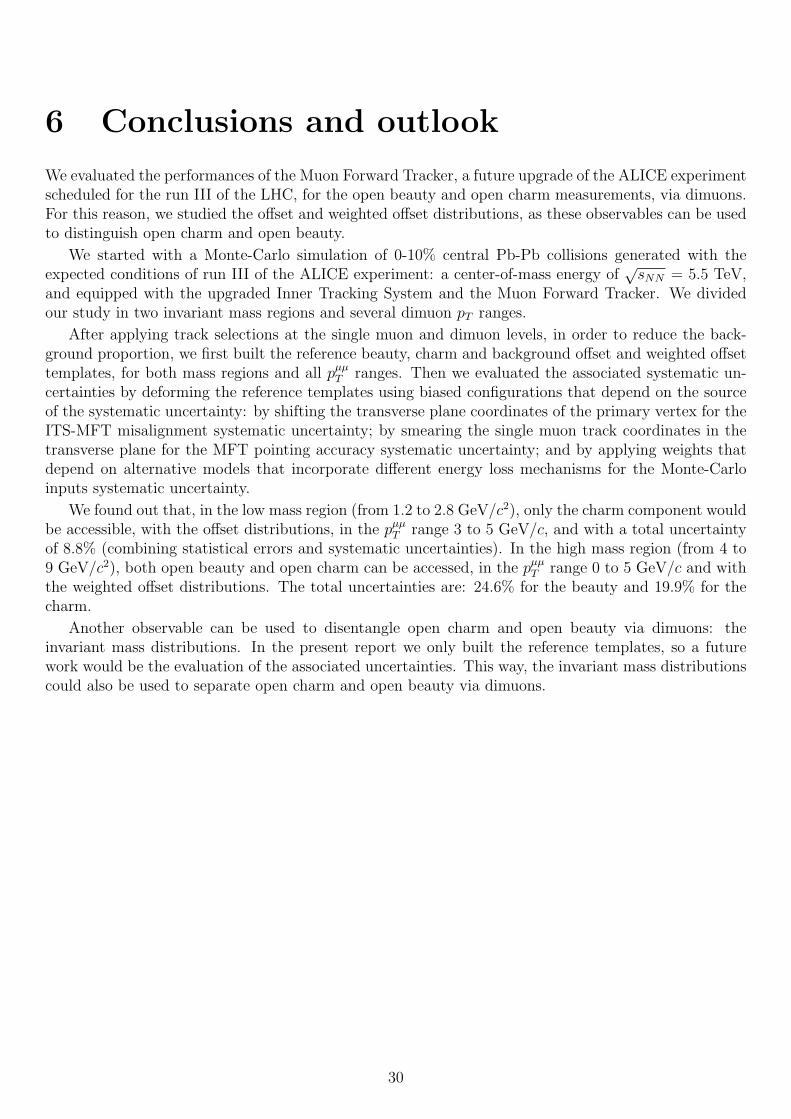
Figure 4.2 shows all the reference offset templates in the low mass region for all four pµµT ranges.

Figure 4.3 shows all the reference weighted offset templates for the low mass region for all four pµµT

ranges.

Figure 4.4 shows the reference offset and weighted offset templates for the high mass region.

19

Low mass region High mass region

pµµT (GeV/c)

statistic (× 103)pµµ

T (GeV/c)statistic (× 103)

beauty charm background beauty charm background0-1 36 1 400 15 800

0-5 606 652 5 4421-2 76 1 940 24 8002-3 124 1 300 19 6003-5 192 593 9 470

Table 4.2: Expected statistics for the three sources, assuming an integrated luminosity of 10 nb−1, forall pµµ

T ranges and both mass regions[9].

Offset (cm)0 0.02 0.04 0.06 0.08 0.1 0.12 0.14 0.16 0.18 0.2

dN

210

310

410

510

610All tracks

beauty← µµ charm← µµ background← µµ

Non-weighted offsets

Quadratic sum of offsets2Low Mass Region : 1.2 to 2.8 GeV/c

range : 0 to 1 GeV/cT

p

Offset (cm)0 0.02 0.04 0.06 0.08 0.1 0.12 0.14 0.16 0.18 0.2

dN

210

310

410

510

610 All tracks beauty← µµ charm← µµ background← µµ




p

Offset (cm)0 0.02 0.04 0.06 0.08 0.1 0.12 0.14 0.16 0.18 0.2

dN

210

310

410

510

610All tracks





p

Offset (cm)0 0.02 0.04 0.06 0.08 0.1 0.12 0.14 0.16 0.18 0.2

dN

310

410

510





p

Figure 4.2: Reference offset templates in the low mass region for each source. The pµµT ranges are: 0

to 1 GeV/c (top left), 1 to 2 GeV/c (top right), 2 to 3 GeV/c (bottom left) and 3 to 5 GeV/c (bottomright). Note that all of these offset distributions are scaled to an integrated luminosity of 10 nb−1.

20

Weighted Offset0 5 10 15 20 25 30

∆dN

/d

10

210

310

410

510

610All tracks


Weighted offsets



p


∆dN

/d

10

210

310

410

510


Weighted offsets



p


∆dN

/d

210

310

410

510

610All tracks


Weighted offsets



p


∆dN

/d

210

310

410

510

610All tracks


Weighted offsets



p

Figure 4.3: Reference weighted offset templates for the low mass region for the pµµT ranges: 0 to 1 GeV/c

(top left), 1 to 2 GeV/c (top right), 2 to 3 GeV/c (bottom left) and 3 to 5 GeV/c (bottom right). Notethat all of these weighted offset distributions are scaled to an integrated luminosity of 10 nb−1.

Offset (cm)0 0.02 0.04 0.06 0.08 0.1 0.12 0.14 0.16 0.18 0.2

dN

310

410

510

All tracks beauty← µµ charm← µµ background← µµ


Quadratic sum of offsets2High Mass Region : 4 to 9 GeV/c


p


∆dN

/d

310

410

510


Weighted offsets

Quadratic sum of offsets2High Mass Region : 4 to 9 GeV/c


p

Figure 4.4: Refrence offset (left) and weighted offset (right) templates for the high mass region for thepµµ

T range 0 to 5 GeV/c. Note that all of these offset and weighted offset distributions are scaled to anintegrated luminosity of 10 nb−1.

21

Invariant mass analysis

In addition to the offset, there exists another observable that can be used to distinguish open beautyand open charm: the invariant mass distributions. We performed the same analysis as described abovefor the offset and weighted offset but for the invariant mass distributions, in both mass regions. Thesteps are the same: we apply the same single muon and dimuon cuts, parametrization, smoothing andscaling to the expected statistic with a 10 nb−1 integrated luminosity. The smoothed invariant masstemplates for both mass regions are shown in figure 4.5.

)2Invariant Mass (GeV/c1.2 1.4 1.6 1.8 2 2.2 2.4 2.6 2.8

dN

310

410

510

610


2Low Mass Region : 1.2 to 2.8 GeV/c


p


dN

410

510

610


2Low Mass Region : 1.2 to 2.8 GeV/c range : 1 to 2 GeV/c

Tp


dN

310

410

510

610

710All tracks


2Low Mass Region : 1.2 to 2.8 GeV/c range : 2 to 3 GeV/c

Tp


dN

410

510

610




p

)2Invariant Mass (GeV/c4 4.5 5 5.5 6 6.5 7 7.5 8 8.5 9

dN

310

410

510


2High Mass Region : 4 to 9 GeV/c


p

Figure 4.5: Reference invariant mass templates in both mass regions for each source. The three topplots and the bottom left plot are for the low mass region, in the pµµ

T ranges: 0 to 1 (top left), 1 to 2 (topmiddle), 2 to 3 (top right) and 3 to 5 GeV/c (bottom left). On the bottom right are the distributions forthe high mass region, in the pµµ

T range 0 to 5 GeV/c. Note that all of these invariant mass distributionsare scaled to an integrated luminosity of 10 nb−1.

4.4 Uncertainties estimation

In order to determine which observable (offset or weighted offset) is the best suited to distinguish openbeauty and open charm, we need to evaluate the uncertainties for each one. This way, we’ll chosethe observable that gives the smallest uncertainties, and so, will be the most accurate for the openbeauty/charm distinction. The total uncertainties in each case are the quadratic sums of the statisticalerrors and all the systematic uncertainties.

4.4.1 Systematic uncertainties

We have three sources of systematic uncertainties:

• A misalignement between the ITS and the MFT;• The limited MFT pointing accuracy;• Different Monte-Carlo inputs;

22

For each of them we’ll re-compute all the single muon offsets and weighted offsets but with a differentconfiguration that depends on the source of the systematic uncertainty. From there we re-compute aset of distorted dimuon offsets and weighted offsets, and then we divide them by the reference ones(Distorted/Reference). Then we parametrize this ratio using polynomial functions, and we use thesefunctions to deform the reference templates. Some of the systematic uncertainties described in thefollowing have ratios in pµµ

T ranges that cover more than one of the pµµT bin from section 4.1.2, in these

cases, the same parametrization function is used across all the reference pµµT bins that are covered. For

example if the ratio is performed for pµµT = 2-5 GeV/c, then the parametrization function obtained will

be multiplied by both “reference” templates for pµµT = 2-3 GeV/c and pµµ

T = 3-5 GeV/c ranges.

In the high mass region, for the ITS-MFT misalignement and MFT pointing accuracy systematicuncertainties, and due to the lack of statistic, we performed the ratios for the sum of the charm and thebackground. However, this is the case only for the ratios: we applied the same fit function to distortseparately the charm and background “reference” templates.

ITS-MFT misalignment

We chose a realistic 10 µm misalignment between the MFT and the ITS. The primary vertex coordinatesare shifted by 10 µm in both x and y directions, and in two cases, either + or - 10 µm:

First case:

{xvertex → xvertex + 10 µm

yvertex → yvertex + 10 µmSecond case:

{xvertex → xvertex − 10 µm

yvertex → yvertex − 10 µm

We performed this analysis in a 0 to 5 GeV/c pµµT range, in both mass regions and for both offset and

weighted offset distributions, as the misalignment does not depend on the pT of the tracks. A fewparametrizations of the ratios Distorted/Reference are shown in figure 4.6.

Offset (cm)0 0.02 0.04 0.06 0.08 0.1 0.12 0.14 0.16 0.18 0.2

Dis

tort

ion

0.975

0.98

0.985

0.99

0.995

1

1.005beauty

charm

background


Dis

tort

ion

0.975

0.98

0.985

0.99

0.995

1

1.005 beauty

charm

background

Offset (cm)0 0.02 0.04 0.06 0.08 0.1 0.12 0.14 0.16 0.18 0.2

Dis

tort

ion

0.93

0.94

0.95

0.96

0.97

0.98

0.99

1

1.01

beauty

charm and background

Figure 4.6: Examples of the parametrizations Distorted/Reference for the ITS-MFT misalignment sys-tematic uncertainty for the three sources, in the pµµ

T range 0 to 5 GeV/c and for a + 10 µm misalign-ment. The left and middle plots are for the low mass region: for the offset (left) and the weightedoffset (middle). The plot on the right is for the offset in the high mass region. In the high mass regionthe parametrization, in order to constraint the fit, corresponds to the sum of charm and backgroundcontributions.

MFT pointing accuracy

The MFT will have a limited pointing accuracy that will depend on the single muons’ pT . The figure 4.7shows the future MFT pointing accuracy resolution, in both x and y directions, as a function of the pµ

T .To reproduce this effect, we smeared the single muons’ coordinates x and y in the transverse plane usinga Gaussian function with a pµ

T dependent width that reflects the MFT pointing accuracy. We take as

23

a width one third of the MFT pointing accuracy in each pµT range, in order to cover the MFT pointing

accuracy within three sigmas, which represents more than 99.7% of the cases. These widths are listedin the table 4.3.

Figure 4.7: The MFT pointing accuracy as a func-tion of the single muon pT (pµ

T ), in both x and ydirections[8].

pµT (GeV/c) σ (µm)0.5 to 1 401 to 1.5 301.5 to 3 20> 3 10

Table 4.3: Gaussian widths for the muontrack smearing chosen in each single muonpT range.

In the low mass region, we performed the ratios for several pµµT ranges, but we need enough statistic in

order to constraint the parametrizations to the ratios Distorted/Reference, so we have chosen these pµµT

ranges:

• beauty: 0-3 and 3-5 GeV/c;• charm and background: 0-1, 1-2 and 2-5 GeV/c;

In the high mass region, the only pµµT range is: 0 to 5 GeV/c. A few parametrizations of the ratios

Distorted/Reference are shown in figure 4.8.

Offset (cm)0 0.02 0.04 0.06 0.08 0.1 0.12 0.14 0.16 0.18 0.2

Dis

tort

ion

0.8

0.85

0.9

0.95

1

1.05

beauty

charm

background


Dis

tort

ion

0.8

0.85

0.9

0.95

1

beauty

charm

background


Dis

tort

ion

0.88

0.9

0.92

0.94

0.96

0.98

1

beauty


Figure 4.8: Examples of the parametrizations Distorted/Reference for the MFT pointing accuracy sys-tematic uncertainty for the three sources. The left and middle plots are for the low mass region in thepµµ

T range 3 to 5 GeV/c: for the offset (left) and the weighted offset (middle). The plot on the right isfor the weighted offset in the high mass region and in the pµµ

T range 0 to 5 GeV/c. In the high massregion, charm and background are added in order to obtain a unique parametrization.

Monte-Carlo inputs

We used as Monte-Carlo generators AliGenCorrHF and HIJING, but there exist other event generatorsfor the same processes. In order to quantify the systematic uncertainties coming from these different

24

Monte-Carlo inputs, we will weight, at the single muon level, the charm and beauty offset and weightedoffset distributions as:

Weight = (FONLL/AliGenCorrHF)×RAA(alternative model)

where FONLL means “Fixed Order Next to Leading Log” and is a pQCD model for heavyquark production, AliGenCorrHF is the generator we use for the open heavy flavors and theRAA(alternative model) is the nuclear modification factor of an alternative model for a given source(open beauty or open charm). The FONLL framework has proven to be successful to predict heavyquark production in proton-proton collisions[10]. The RAA models take into account heavy ion colli-sions’ nuclear effects (radiative and/or collisional energy loss). The RAA plots for each alternative modelsare available in figures A.13, A.14, A.15 and A.16 in the appendix. The list of alternative models thatwe used for beauty and charm are:

• beauty: Uphoff, HeM, HTLTH155;• charm: POWLANG, MCHQEPOS and MCHQEPOSRadLPM;

The “reference” histograms, only for the Monte-Carlo inputs systematic uncertainties and only for thebeauty and the charm, are no longer the ones described in section 4.3, but the ones obtained by applyingthe weight with the following models:

• beauty: LatQCDTH155;• charm: TAMU;

We chose those models because they have the best descriptions of the ALICE data. The LatQCDTH155and TAMU offset and weighted offset distributions have been processed with the same approach asdescribed earlier for the “reference” templates: parametrization, smoothing and scaling to 10 nb−1 inboth mass regions and across all pµµ

T ranges.

For the background, since it is composed of a lot of different kind of particles, there is no globalmodel for it. We used as “reference” histograms for the background the distributions obtained withoutany distortion (section 4.3). To obtain the two “alternative models” for the background, we appliedthese weights at the single muon level:

• First weight: 0.5 + (1/10 · pµT );

• Second weight: 1.5 - (1/10 · pµT );

Finally, the weight at the dimuon level, for the three sources, is the multiplication of the two singlemuon weights that form the pair: (weight µ1) · (weight µ2).

Then we divide the offset and weighted offset distributions obtained with a different model by the“reference” distributions. We select in each case the alternative model that gives the largest deviationfrom unity and parametrize the corresponding ratio with polynomial functions. The models that gavethe largest deviations are:

• For the beauty: Uphoff;• For the charm: POWLANG, except for the offset in the pµµ

T range 1-2 GeV/c and the weightedoffset in pµµ

T range 2-5 GeV/c in which it is for the two cases MCHQEPOSRadLPM;• For the background: 0.5 + (1/10 · pµ

T );

The pµµT range in which we perfomed the ratios are: in the low mass region we chose 0-3 anf 3-5 GeV/c

25

for the beauty and 0-1, 1-2 and 2-5 GeV/c for the charm and the background; in the high mass regionit is 0 to 5 GeV/c in all cases.

Figure 4.9 shows a few parametrizations of the ratios Distorted/Reference.

Offset (cm)0 0.02 0.04 0.06 0.08 0.1 0.12 0.14 0.16 0.18 0.2

Dis

tort

ion

0.85

0.9

0.95

1

1.05

beauty

charm

background


Dis

tort

ion

0.8

0.85

0.9

0.95

1

1.05

1.1beauty

charm

background

Offset (cm)0 0.02 0.04 0.06 0.08 0.1 0.12 0.14 0.16 0.18 0.2

Dis

tort

ion

0.85

0.9

0.95

1

1.05

1.1

beauty

charm

background

Figure 4.9: Examples of the parametrizations Distorted/Reference for the Monte-Carlo input systematicuncertainties for the three sources. The plots on the left and in the middle are for the low mass region,in the pµµ

T range 3 to 5 GeV/c: for the offset (left) and the weighted offset (middle). The plot on theright is for the offset in the high mass region, in the pµµ

T range 0 to 5 GeV/c.

Final step

We obtain the “distorted” templates, for each systematic uncertainty source, mass region and pµµT range,

by mutliplying the parametrized ratios Distorted/Reference by the “reference” templates.

These “distorted” templates are then used to fit the total reference (sum of charm, beauty and back-ground) offset and weighted offset distributions in each pµµ

T range. The fit function is the superpositionof the three expected constributions:

F = C · fcharm + B · fbeauty + D · fbackground (4.1)

where fcharm, fbeauty and fbackground are the “distorted” templates for charm, beauty and backgroundrespectively. In the same way, B, C and D are the free parameters corresponding to the normalizationof the three components.

The systematic uncertainties are then obtained for the beauty and the charm as:

Systematic uncertainty = |1− (Integral of the distorted distribution)

(Integral of the reference distribution)|

In the end the total systematic uncertainty is the quadratic sum of the three systematic uncertainties.

4.4.2 Statistical errors

In addition to the systematic uncertainties we also need to quantify the statistical errors. We’ll usea similar approach as for the systematic uncertainties: we fit the total “reference” distribution usingfunction 4.1 that is now the sum of the three “reference” components and not the “distorted” ones. Weevaluate the statistical errors as:

Statistical error = (Parameter error)/(Integral of the reference distribution)

26

5 Results

We’ll present and discuss the statistical errors, the systematic uncertainties and the total uncertainties,for each source, each pµµ

T range and mass region.

5.1 Statistical errors and systematic uncertainties

Systematic uncertainties

All the systematic uncertainties, for the low mass region, are shown in table 5.1 (offset) and in table 5.2(weighted offset). Table 5.3 contains all the systematic uncertainties for the high mass region.

pµµT (GeV/c)

Systematic uncertainties for the offset in the low mass regionITS-MFT misalignment MFT pointing accuracy Monte-Carlo inputs

beauty charmbeauty charm beauty charm

+10µm -10µm +10µm -10µm0-1 95.5% − 0.5% 8.4% − 65.9% − 7.1%1-2 − − 0.6% 8.6% − 51.4% − 13.7%2-3 − − 3.4% 5.6% − 67.0% − 2.9%3-5 30.5% − 1.9% 2.1% − 7.6% − 2.5%

Table 5.1: Table of the systematic uncertainties in the low mass region for the offset. For each case, thelargest ITS-MFT misalignment uncertainty is in bold. A hyphen indicates that uncertainty could notbe quantified.

pµµT (GeV/c)

Systematic uncertainties for the weighted offset in the low mass regionITS-MFT misalignment MFT pointing accuracy Monte-Carlo inputs

beauty charmbeauty charm beauty charm

+10µm -10µm +10µm -10µm0-1 − − 1.9% 8.5% − 60.6% − 11.0%1-2 − − 3.2% 3.0% − 34.4% − 0.6%2-3 − − 6.1% 8.9% − − − 1.9%3-5 34.6% − 6.7% 7.5% − − − 8.8%

Table 5.2: Table of the systematic uncertainties in the low mass region for the weighted offset. For eachcase, the largest ITS-MFT misalignment uncertainty is in bold. A hyphen indicates that uncertaintycould not be quantified.

27

Observable

Systematic uncertainties in the high mass region (pµµT range: 0-5 GeV/c)

ITS-MFT misalignment MFT pointing accuracy Monte-Carlo inputsbeauty charm

beauty charm beauty charm+10µm -10µm +10µm -10µm

Offset 39.3% 24.4% 20.4% 13.2% − 45.7% 46.3% 27.7%Weighted offset 8.0% 1.8% 7.2% 1.4% 3.6% 11.1% 22.6% 14.6%

Table 5.3: Table of the systematic uncertainties in the high mass region for the offset and weightedoffset. For each case, the largest ITS-MFT misalignment uncertainty is in bold. A hyphen indicatesthat uncertainty could not be quantified.

Statistical errors and total systematic uncertainties

The statistical errors and the total systematic uncertainties for the low mass region are in table 5.4.The proper high mass region results are in table 5.5. For the ITS-MFT misalignment we have two cases:+ 10 µm or - 10 µm. In order to be conservative, we’ll pick, in each situation, the case that gives thelargest systematic uncertainty.

Statistical errors and total systematic uncertainties in the low mass region

pµµT (GeV/c)

Offset Weighted offset

Statistical errorsTotal systematic

Statistical errorsTotal systematic

uncertainties uncertaintiesbeauty charm beauty charm beauty charm beauty charm

0-1 − 0.7% − 66.9% − 1.0% − 62.2%1-2 81.8% 0.5% − 53.9% 92.8% 0.9% − 34.6%2-3 55.7% 1.6% − 67.3% 45.1% 1.8% − −3-5 34.5% 2.8% − 8.3% 23.6% 3.9% − −

Table 5.4: Table of the statistical errors and total systematic uncertainties in the low mass region forthe offset and weighted offset. A hyphen indicates that uncertainty could not be quantified.

Statistical errors and total systematic uncertainties in the high mass region

ObservableStatistical errors Total systematic uncertainties

beauty charm beauty charmOffset 2.7% 1.1% − 57.3%

Weighted offset 3.2% 1.7% 24.3% 19.8%

Table 5.5: Table of the statistical errors and total systematic uncertainties in the high mass region, inthe pµµ

T range 0-5 GeV/c and for the offset and weighted offset. A hyphen indicates that uncertaintycould not be quantified.

Total uncertainties

The total uncertainties (quadratic sums of the statistical errors and total systematic uncertainties) forall cases are in table 5.6.

28

Total uncertainties in the low mass region Total uncertainties in the high mass region

pµµT (GeV/c)

Offset Weighted offsetpµµ

T (GeV/c)Offset Weighted offset

beauty charm beauty charm beauty charm beauty charm0-1 − 67.0% − 62.3%

0-5 − 57.4% 24.6% 19.9%1-2 − 54.0% − 34.7%2-3 − 67.4% − −3-5 − 8.8% − −

Table 5.6: Table of the total uncertainties (statistical and systematic) in both mass regions and for theoffset and weighted offset. A hyphen indicates that uncertainty could not be quantified.

5.2 Discussion

Low mass region

In the low mass region, in most cases the systematic uncertainties could not be determined or are verylarge, even for the ITS-MFT misalignment where the distortions are very small (as visible on the plots infigure 4.6), for both open beauty and open charm. In order to understand why, and given the fact thatthe background is dominating in every pµµ

T range in the low mass region (as visible on the “reference”templates in figures 4.2 and 4.3 in section 4.3), we tried to evaluate its impact on the systematicuncertainties. We performed the same systematic uncertainties evaluation process described earlier forthe ITS-MFT misalignment case, but this time we did not apply any distortion to the background.Table 5.7 shows the uncertainties obtained.

pµµT (GeV/c)

ITS-MFT misalignment uncertainties wihtout background distortionOffset Weighted offset

beauty charm beauty charm+10µm -10µm +10µm -10µm +10µm -10µm +10µm -10µm

0-1 2.6% 48.3% 0.4% 0.6% 28.3% 3.7% 0.4% 0.6%1-2 58.0% − 0.3% 0.5% − − 0.6% 0.7%2-3 32.5% 79.0% 0.9% 1.3% 52.9% 56.0% 1.6% 1.7%3-5 10.8% 37.5% 0.8% 2.0% 13.7% 18.1% 1.9% 2.5%

Table 5.7: Table of the ITS-MFT misalignment systematic uncertainties in the low mass region for theoffset and weighted offset distributions, without any distortion applied to the background. In each case,the largest uncertainty is in bold. A hyphen indicates that uncertainty could not be quantified. Theuncertainties obtained here are smaller and are available in more cases.

The ITS-MFT misalignment systematic uncertainties obtained without distorting the background inthe low mass region are smaller in all cases. We have results for all pµµ

T ranges for the charm and almostall of them for the beauty. Moreover, the charm systematic uncertainties have dropped considerably,down to 2.5% at maximum. We concluded that, in the low mass region, the background is so large thatit avoids measuring both open beauty and open charm via dimuons in most cases.

The global MFT performance for open heavy flavor measurements via dimuons

In the end, the open beauty via dimuons will not be accessible in the low mass region, only open charmwill be measurable, in the pµµ

T range 3 to 5 GeV/c, using the offset distributions, and with a totaluncertainty of ∼8.8%.

In the high mass region, both open beauty and open charm will be accessible via dimuons, in thepµµ

T range 0 to 5 GeV/c, with the weighted offset distributions and with total uncertainties of ∼24.6%and ∼19.9% respectively.

29

6 Conclusions and outlook

We evaluated the performances of the Muon Forward Tracker, a future upgrade of the ALICE experimentscheduled for the run III of the LHC, for the open beauty and open charm measurements, via dimuons.For this reason, we studied the offset and weighted offset distributions, as these observables can be usedto distinguish open charm and open beauty.

We started with a Monte-Carlo simulation of 0-10% central Pb-Pb collisions generated with theexpected conditions of run III of the ALICE experiment: a center-of-mass energy of

√sNN = 5.5 TeV,

and equipped with the upgraded Inner Tracking System and the Muon Forward Tracker. We dividedour study in two invariant mass regions and several dimuon pT ranges.

After applying track selections at the single muon and dimuon levels, in order to reduce the back-ground proportion, we first built the reference beauty, charm and background offset and weighted offsettemplates, for both mass regions and all pµµ

T ranges. Then we evaluated the associated systematic un-certainties by deforming the reference templates using biased configurations that depend on the sourceof the systematic uncertainty: by shifting the transverse plane coordinates of the primary vertex for theITS-MFT misalignment systematic uncertainty; by smearing the single muon track coordinates in thetransverse plane for the MFT pointing accuracy systematic uncertainty; and by applying weights thatdepend on alternative models that incorporate different energy loss mechanisms for the Monte-Carloinputs systematic uncertainty.

We found out that, in the low mass region (from 1.2 to 2.8 GeV/c2), only the charm component wouldbe accessible, with the offset distributions, in the pµµ

T range 3 to 5 GeV/c, and with a total uncertaintyof 8.8% (combining statistical errors and systematic uncertainties). In the high mass region (from 4 to9 GeV/c2), both open beauty and open charm can be accessed, in the pµµ

T range 0 to 5 GeV/c and withthe weighted offset distributions. The total uncertainties are: 24.6% for the beauty and 19.9% for thecharm.

Another observable can be used to disentangle open charm and open beauty via dimuons: theinvariant mass distributions. In the present report we only built the reference templates, so a futurework would be the evaluation of the associated uncertainties. This way, the invariant mass distributionscould also be used to separate open charm and open beauty via dimuons.

30

Bibliography

[1] Francis Halzen and Alan D. Martin. Quarks and leptons: An Introductory Course in ModernParticle Physics. Wiley; 1st edition (January 20, 1984), 1984.

[2] J. Beringer et al (Particle Data Group). Review of particle physics. Phys. Rev., D86:010001, 2012.

[3] Lizardo Valencia Palomo. Inclusive J/psi production measurement in Pb-Pb collisions at√sNN =

2.76 TeV with the ALICE Muon Spectrometer. Theses, Universite Paris Sud - Paris XI, September2013.

[4] Loic Manceau. Mesure de la section efficace de production des hadrons lourds avec le spectrometrea muons d’ALICE au LHC. PhD thesis, 2010. These de doctorat dirigee par Crochet, PhilippePhysique Corpusculaire Clermont-Ferrand 2 2010.

[5] X. Zhang. Study of Heavy Flavours from Muons Measured with the ALICE Detector in Proton-Proton and Heavy-Ion Collisions at the CERN-LHC. Theses, Universite Blaise Pascal - Clermont-Ferrand II, May 2012. N d’ordre: DU 2240 EDSF : 714.

[6] The ALICE Collaboration. The alice experiment at the cern lhc. Journal of Instrumentation,3(08):S08002, 2008.

[7] B Abelev et al and The ALICE Collaboration. Technical design report for the upgrade of the aliceinner tracking system. Journal of Physics G: Nuclear and Particle Physics, 41(8):087002, 2014.

[8] Technical Design Report for the Muon Forward Tracker. Technical Report CERN-LHCC-2015-001.ALICE-TDR-018, CERN, Geneva, Jan 2015.

[9] Addendum of the Letter Of Intent for the Upgrade of the ALICE Experiment : The Muon ForwardTracker. Technical Report CERN-LHCC-2013-014. LHCC-I-022-ADD-1, CERN, Geneva, Aug 2013.

[10] Matteo Cacciari, Stefano Frixione, Nicolas Houdeau, Michelangelo L. Mangano, Paolo Nason, et al.Theoretical predictions for charm and bottom production at the LHC. JHEP, 1210:137, 2012.

31

A Appendix

Offset and weighted offset parametrizations

/ ndf 2χ 70.79 / 68norm 3.9± 102.3 mean 0.00263± 0.02468

L0σ 0.00572± 0.01669 L

1σ 0.1924± -0.3612 R

0σ 0.00531± 0.02702 R

1σ 0.0907± 0.2086 R

2σ 0.42347± -0.06541

Offset (cm)0 0.02 0.04 0.06 0.08 0.1 0.12 0.14 0.16 0.18 0.2

dN

0

20

40

60

80

100

120

140 / ndf 2χ 70.79 / 68

norm 3.9± 102.3 mean 0.00263± 0.02468

L0σ 0.00572± 0.01669 L

1σ 0.1924± -0.3612 R

0σ 0.00531± 0.02702 R

1σ 0.0907± 0.2086 R

2σ 0.42347± -0.06541

from beautyµµ


Quadratic sum of offsets


range : 0 to 1 GeV/cµµT

p

/ ndf 2χ 87.59 / 67norm 7.1± 321.6 mean 0.00153± 0.02219

L0σ 0.0031± 0.0119 L

1σ 0.1307± -0.2372 R

0σ 0.00301± -0.02674 R

1σ 0.0512± -0.2196 R

2σ 0.2369± 0.1117

Offset (cm)0 0.02 0.04 0.06 0.08 0.1 0.12 0.14 0.16 0.18 0.2

dN

0

50

100

150

200

250

300

350

/ ndf 2χ 87.59 / 67norm 7.1± 321.6 mean 0.00153± 0.02219

L0σ 0.0031± 0.0119 L

1σ 0.1307± -0.2372 R

0σ 0.00301± -0.02674 R

1σ 0.0512± -0.2196 R

2σ 0.2369± 0.1117

from beautyµµ





p

/ ndf 2χ 78.98 / 69norm 6.6± 325.5 mean 0.00174± 0.02441

L0σ 0.00495± 0.02062 L

1σ 0.1658± -0.5651 R

0σ 0.0013± 0.0226 R

1σ 0.009± 0.247

Offset (cm)0 0.02 0.04 0.06 0.08 0.1 0.12 0.14 0.16 0.18 0.2

dN

0

50

100

150

200

250

300

350

/ ndf 2χ 78.98 / 69norm 6.6± 325.5 mean 0.00174± 0.02441

L0σ 0.00495± 0.02062 L

1σ 0.1658± -0.5651 R

0σ 0.0013± 0.0226 R

1σ 0.009± 0.247

from beautyµµ





p

/ ndf 2χ 49.02 / 43norm 10.8± 553.3 mean 0.00189± 0.02021

L0σ 0.00479± 0.01664 L

1σ 0.1787± -0.5596 R

0σ 0.00258± -0.02294 R

1σ 0.041± -0.233 R

2σ 0.18139± 0.01758

Offset (cm)0 0.02 0.04 0.06 0.08 0.1 0.12 0.14 0.16 0.18 0.2

dN

0

100

200

300

400

500

600 / ndf 2χ 49.02 / 43

norm 10.8± 553.3 mean 0.00189± 0.02021

L0σ 0.00479± 0.01664 L

1σ 0.1787± -0.5596 R

0σ 0.00258± -0.02294 R

1σ 0.041± -0.233 R

2σ 0.18139± 0.01758

from beautyµµ





p

Figure A.1: Offset parametrizations for the beauty, in the low mass region, in pµµT ranges: 0 to 1 GeV/c

(top left), 1 to 2 GeV/c (top right), 2 to 3 GeV/c (bottom left) and 3 to 5 GeV/c (bottom right). Notethat all of these offset distributions are not scaled to an integrated luminosity of 10 nb−1.

32

/ ndf 2χ 128 / 68norm 10.0± 445.2 mean 0.00107± 0.01741

L0σ 0.001981± -0.009004 L

1σ 0.0997± 0.2463 R

0σ 0.00163± -0.01622 R

1σ 0.0334± -0.2364 R

2σ 0.183± 0.165

Offset (cm)0 0.02 0.04 0.06 0.08 0.1 0.12 0.14 0.16 0.18 0.2

dN

0

100

200

300

400

500

/ ndf 2χ 128 / 68norm 10.0± 445.2 mean 0.00107± 0.01741

L0σ 0.001981± -0.009004 L

1σ 0.0997± 0.2463 R

0σ 0.00163± -0.01622 R

1σ 0.0334± -0.2364 R

2σ 0.183± 0.165

from charmµµ





p

/ ndf 2χ 101.7 / 68norm 13.9± 774 mean 0.00061± 0.01647

L0σ 0.001137± 0.008163 L

1σ 0.0607± -0.2069 R

0σ 0.00081± -0.01276 R

1σ 0.018± -0.283 R

2σ 0.1041± 0.3367

Offset (cm)0 0.02 0.04 0.06 0.08 0.1 0.12 0.14 0.16 0.18 0.2

dN

0

100

200

300

400

500

600

700

800

/ ndf 2χ 101.7 / 68norm 13.9± 774 mean 0.00061± 0.01647

L0σ 0.001137± 0.008163 L

1σ 0.0607± -0.2069 R

0σ 0.00081± -0.01276 R

1σ 0.018± -0.283 R

2σ 0.1041± 0.3367

from charmµµ





p

/ ndf 2χ 62.91 / 64norm 10.9± 341.2 mean 0.00079± 0.01368

L0σ 0.001285± 0.005877 L

1σ 0.0854± -0.1319 R

0σ 0.00114± 0.01083 R

1σ 0.0289± 0.2874 R

2σ 0.1912± -0.3837

Offset (cm)0 0.02 0.04 0.06 0.08 0.1 0.12 0.14 0.16 0.18 0.2

dN

0

50

100

150

200

250

300

350

400 / ndf 2χ 62.91 / 64

norm 10.9± 341.2 mean 0.00079± 0.01368

L0σ 0.001285± 0.005877 L

1σ 0.0854± -0.1319 R

0σ 0.00114± 0.01083 R

1σ 0.0289± 0.2874 R

2σ 0.1912± -0.3837

from charmµµ





p

/ ndf 2χ 16.85 / 31norm 11.5± 243.2 mean 0.00149± 0.01189

L0σ 0.002638± 0.005955 L

1σ 0.1890± -0.1945 R

0σ 0.002307± 0.009341 R

1σ 0.0908± 0.2982 R

2σ 1.2414± -0.7329 R

3σ 5.041± 2.411

Offset (cm)0 0.02 0.04 0.06 0.08 0.1 0.12 0.14 0.16 0.18 0.2

dN

0

50

100

150

200

250

/ ndf 2χ 16.85 / 31norm 11.5± 243.2 mean 0.00149± 0.01189

L0σ 0.002638± 0.005955 L

1σ 0.1890± -0.1945 R

0σ 0.002307± 0.009341 R

1σ 0.0908± 0.2982 R

2σ 1.2414± -0.7329 R

3σ 5.041± 2.411

from charmµµ





p

Figure A.2: Offset parametrizations for the charm, in the low mass region, in pµµT ranges: 0 to 1 GeV/c

(top left), 1 to 2 GeV/c (top right), 2 to 3 GeV/c (bottom left) and 3 to 5 GeV/c (bottom right). Notethat all of these offset distributions are not scaled to an integrated luminosity of 10 nb−1.

/ ndf 2χ 93.7 / 67norm 14.2± 1181 mean 0.00113± 0.02441

L0σ 0.00249± 0.01772 L

1σ 0.076± -0.475 R

0σ 0.00292± 0.02397 R

1σ 0.0804± 0.2723 R

2σ 0.8055± -0.7424 R

3σ 2.601± 3.301

Offset (cm)0 0.02 0.04 0.06 0.08 0.1 0.12 0.14 0.16 0.18 0.2

dN

0

200

400

600

800

1000

1200

/ ndf 2χ 93.7 / 67norm 14.2± 1181 mean 0.00113± 0.02441

L0σ 0.00249± 0.01772 L

1σ 0.076± -0.475 R

0σ 0.00292± 0.02397 R

1σ 0.0804± 0.2723 R

2σ 0.8055± -0.7424 R

3σ 2.601± 3.301

from backgroundµµ





p

/ ndf 2χ 71.09 / 67norm 14.7± 1176 mean 0.0010± 0.0214

L0σ 0.00210± 0.01451 L

1σ 0.0758± -0.4137 R

0σ 0.00236± -0.02173 R

1σ 0.066± -0.416 R

2σ 0.676± 2.341 R

3σ 2.213± -8.444

Offset (cm)0 0.02 0.04 0.06 0.08 0.1 0.12 0.14 0.16 0.18 0.2

dN

0

200

400

600

800

1000

1200

/ ndf 2χ 71.09 / 67norm 14.7± 1176 mean 0.0010± 0.0214

L0σ 0.00210± 0.01451 L

1σ 0.0758± -0.4137 R

0σ 0.00236± -0.02173 R

1σ 0.066± -0.416 R

2σ 0.676± 2.341 R

3σ 2.213± -8.444

from backgroundµµ





p

/ ndf 2χ 59.48 / 67norm 9.4± 382.6 mean 0.00164± 0.01939

L0σ 0.00417± 0.01623 L

1σ 0.160± -0.578 R

0σ 0.00291± -0.01413 R

1σ 0.0866± -0.4754 R

2σ 0.94± 2.09 R

3σ 3.179± -5.621

Offset (cm)0 0.02 0.04 0.06 0.08 0.1 0.12 0.14 0.16 0.18 0.2

dN

0

50

100

150

200

250

300

350

400

/ ndf 2χ 59.48 / 67norm 9.4± 382.6 mean 0.00164± 0.01939

L0σ 0.00417± 0.01623 L

1σ 0.160± -0.578 R

0σ 0.00291± -0.01413 R

1σ 0.0866± -0.4754 R

2σ 0.94± 2.09 R

3σ 3.179± -5.621

from backgroundµµ





p

/ ndf 2χ 70.48 / 43norm 8.2± 243 mean 0.00168± 0.01296

L0σ 0.003057± -0.006876 L

1σ 0.1946± 0.2445 R

0σ 0.00322± 0.02401 R

1σ 0.0556± 0.2125 R

2σ 0.2606± 0.0322

Offset (cm)0 0.02 0.04 0.06 0.08 0.1 0.12 0.14 0.16 0.18 0.2

dN

0

50

100

150

200

250

/ ndf 2χ 70.48 / 43norm 8.2± 243 mean 0.00168± 0.01296

L0σ 0.003057± -0.006876 L

1σ 0.1946± 0.2445 R

0σ 0.00322± 0.02401 R

1σ 0.0556± 0.2125 R

2σ 0.2606± 0.0322

from backgroundµµ





p

Figure A.3: Offset parametrizations for the background, in the low mass region, in pµµT ranges: 0 to 1

GeV/c (top left), 1 to 2 GeV/c (top right), 2 to 3 GeV/c (bottom left) and 3 to 5 GeV/c (bottom right).Note that all of these offset distributions are not scaled to an integrated luminosity of 10 nb−1.

33

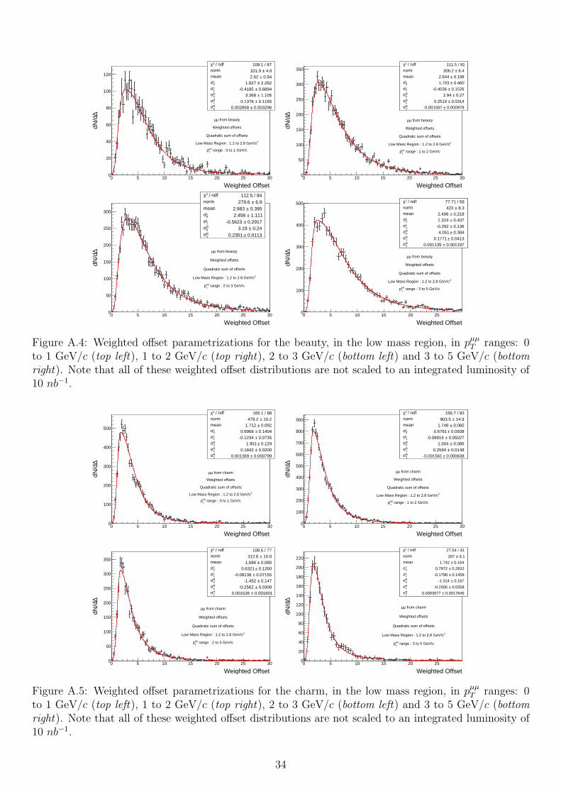
/ ndf 2χ 109.1 / 87norm 4.0± 101.9 mean 0.94± 2.62

L0σ 2.262± 1.827 L

1σ 0.6894± -0.4185 R

0σ 1.105± 3.368 R

1σ 0.1165± 0.1378 R

2σ 0.003296± 0.002858


∆dN

/d

0

20

40

60

80

100

120

/ ndf 2χ 109.1 / 87norm 4.0± 101.9 mean 0.94± 2.62

L0σ 2.262± 1.827 L

1σ 0.6894± -0.4185 R

0σ 1.105± 3.368 R

1σ 0.1165± 0.1378 R

2σ 0.003296± 0.002858

from beautyµµ

Weighted offsets




p

/ ndf 2χ 111.5 / 91norm 6.4± 306.2 mean 0.198± 2.644

L0σ 0.460± 1.703 L

1σ 0.1526± -0.4036 R

0σ 0.27± 2.94 R

1σ 0.0314± 0.2519 R

2σ 0.000978± -0.001567


∆dN

/d

0

50

100

150

200

250

300

350 / ndf 2χ 111.5 / 91

norm 6.4± 306.2 mean 0.198± 2.644

L0σ 0.460± 1.703 L

1σ 0.1526± -0.4036 R

0σ 0.27± 2.94 R

1σ 0.0314± 0.2519 R

2σ 0.000978± -0.001567

from beautyµµ

Weighted offsets




p

/ ndf 2χ 112.5 / 94norm 6.9± 279.6 mean 0.395± 2.983

L0σ 1.111± 2.458 L

1σ 0.2917± -0.5623 R

0σ 0.24± 3.19 R

1σ 0.0113± 0.2301


∆dN

/d

0

50

100

150

200

250

300

/ ndf 2χ 112.5 / 94norm 6.9± 279.6 mean 0.395± 2.983

L0σ 1.111± 2.458 L

1σ 0.2917± -0.5623 R

0σ 0.24± 3.19 R

1σ 0.0113± 0.2301

from beautyµµ

Weighted offsets




p

/ ndf 2χ 77.71 / 59norm 8.3± 423 mean 0.218± 2.406

L0σ 0.407± 1.324 L

1σ 0.136± -0.292 R

0σ 0.384± 4.051 R

1σ 0.0413± 0.1771 R

2σ 0.001197± 0.001135

Weighted Offset0 5 10 15 20 25

∆dN

/d

0

100

200

300

400

500 / ndf 2χ 77.71 / 59norm 8.3± 423 mean 0.218± 2.406

L0σ 0.407± 1.324 L

1σ 0.136± -0.292 R

0σ 0.384± 4.051 R

1σ 0.0413± 0.1771 R

2σ 0.001197± 0.001135

from beautyµµ

Weighted offsets




p

Figure A.4: Weighted offset parametrizations for the beauty, in the low mass region, in pµµT ranges: 0

to 1 GeV/c (top left), 1 to 2 GeV/c (top right), 2 to 3 GeV/c (bottom left) and 3 to 5 GeV/c (bottomright). Note that all of these weighted offset distributions are not scaled to an integrated luminosity of10 nb−1.

/ ndf 2χ 165.1 / 88norm 10.2± 479.2 mean 0.092± 1.712

L0σ 0.1404± 0.6968 L

1σ 0.0735± -0.1234 R

0σ 0.129± 1.951 R

1σ 0.0200± 0.1842 R

2σ 0.000799± 0.001369


∆dN

/d

0

100

200

300

400

500

/ ndf 2χ 165.1 / 88norm 10.2± 479.2 mean 0.092± 1.712

L0σ 0.1404± 0.6968 L

1σ 0.0735± -0.1234 R

0σ 0.129± 1.951 R

1σ 0.0200± 0.1842 R

2σ 0.000799± 0.001369

from charmµµ

Weighted offsets



p

/ ndf 2χ 156.7 / 92norm 14.9± 803.5 mean 0.060± 1.748

L0σ 0.0938± 0.6761 L

1σ 0.05027± -0.08916 R

0σ 0.086± 1.504 R

1σ 0.0148± 0.2594 R

2σ 0.000638± -0.001561


∆dN

/d

0

100

200

300

400

500

600

700

800

900

/ ndf 2χ 156.7 / 92norm 14.9± 803.5 mean 0.060± 1.748

L0σ 0.0938± 0.6761 L

1σ 0.05027± -0.08916 R

0σ 0.086± 1.504 R

1σ 0.0148± 0.2594 R

2σ 0.000638± -0.001561

from charmµµ

Weighted offsets




p

/ ndf 2χ 106.5 / 77norm 10.0± 312.6 mean 0.080± 1.686

L0σ 0.1260± 0.6321 L

1σ 0.07155± -0.08138 R

0σ 0.147± -1.452 R

1σ 0.0308± -0.2562 R

2σ 0.001601± 0.001526


∆dN

/d

0

50

100

150

200

250

300

350

/ ndf 2χ 106.5 / 77norm 10.0± 312.6 mean 0.080± 1.686

L0σ 0.1260± 0.6321 L

1σ 0.07155± -0.08138 R

0σ 0.147± -1.452 R

1σ 0.0308± -0.2562 R

2σ 0.001601± 0.001526

from charmµµ

Weighted offsets




p

/ ndf 2χ 27.54 / 43

norm 9.1± 207 mean 0.164± 1.742

L0σ 0.2832± 0.7972 L

1σ 0.1458± -0.1798 R

0σ 0.187± -1.314 R

1σ 0.0358± -0.2505 R

2σ 0.0017646± 0.0003077


∆dN

/d

0

20

40

60

80

100

120

140

160

180

200

220

/ ndf 2χ 27.54 / 43

norm 9.1± 207 mean 0.164± 1.742

L0σ 0.2832± 0.7972 L

1σ 0.1458± -0.1798 R

0σ 0.187± -1.314 R

1σ 0.0358± -0.2505 R

2σ 0.0017646± 0.0003077

from charmµµ

Weighted offsets




p

Figure A.5: Weighted offset parametrizations for the charm, in the low mass region, in pµµT ranges: 0

to 1 GeV/c (top left), 1 to 2 GeV/c (top right), 2 to 3 GeV/c (bottom left) and 3 to 5 GeV/c (bottomright). Note that all of these weighted offset distributions are not scaled to an integrated luminosity of10 nb−1.

34

/ ndf 2χ 114 / 93norm 13.2± 1324 mean 0.074± 2.188

L0σ 0.157± 1.393 L

1σ 0.0565± -0.3991 R

0σ 0.113± -3.253 R

1σ 0.0137± -0.1013 R

2σ 0.000430± -0.005109


∆dN

/d

0

200

400

600

800

1000

1200

1400

/ ndf 2χ 114 / 93norm 13.2± 1324 mean 0.074± 2.188

L0σ 0.157± 1.393 L

1σ 0.0565± -0.3991 R

0σ 0.113± -3.253 R

1σ 0.0137± -0.1013 R

2σ 0.000430± -0.005109

from backgroundµµ

Weighted offsets




p

/ ndf 2χ 140.5 / 92norm 14.8± 1204 mean 0.074± 2.027

L0σ 0.14± 1.13 L

1σ 0.0564± -0.3003 R

0σ 0.234± -3.048 R

1σ 0.0468± -0.3008 R

2σ 0.00321± 0.01129 R

3σ 0.0000688± -0.0003486


∆dN

/d

0

200

400

600

800

1000

1200

/ ndf 2χ 140.5 / 92norm 14.8± 1204 mean 0.074± 2.027

L0σ 0.14± 1.13 L

1σ 0.0564± -0.3003 R

0σ 0.234± -3.048 R

1σ 0.0468± -0.3008 R

2σ 0.00321± 0.01129 R

3σ 0.0000688± -0.0003486

from backgroundµµ

Weighted offsets




p

/ ndf 2χ 124.3 / 93

norm 7.4± 346.8

mean 0.116± 1.748

L0σ 0.2058± 0.8231

L1σ 0.1037± -0.1941

R0σ 0.225± 3.068

R1σ 0.0276± 0.2114

R2σ 0.0008736± 0.0008193


∆dN

/d

0

50

100

150

200

250

300

350

400

/ ndf 2χ 124.3 / 93

norm 7.4± 346.8

mean 0.116± 1.748

L0σ 0.2058± 0.8231

L1σ 0.1037± -0.1941

R0σ 0.225± 3.068

R1σ 0.0276± 0.2114

R2σ 0.0008736± 0.0008193

from backgroundµµ

Weighted offsets




p

/ ndf 2χ 88.74 / 58norm 8.0± 227.3 mean 0.209± 1.884

L0σ 0.40± 1.04 L

1σ 0.1793± -0.2878 R

0σ 0.270± -2.118 R

1σ 0.0336± -0.3343 R

2σ 0.001136± 0.003074


∆dN

/d

0

50

100

150

200

250 / ndf 2χ 88.74 / 58

norm 8.0± 227.3 mean 0.209± 1.884

L0σ 0.40± 1.04 L

1σ 0.1793± -0.2878 R

0σ 0.270± -2.118 R

1σ 0.0336± -0.3343 R

2σ 0.001136± 0.003074

from backgroundµµ

Weighted offsets




p

Figure A.6: Weighted offset parametrizations for the background, in the low mass region, in pµµT ranges:

0 to 1 GeV/c (top left), 1 to 2 GeV/c (top right), 2 to 3 GeV/c (bottom left) and 3 to 5 GeV/c (bottomright). Note that all of these weighted offset distributions are not scaled to an integrated luminosity of10 nb−1.

/ ndf 2χ 36.41 / 42norm 22.0± 1536 mean 0.00072± 0.01445

L0σ 0.001593± -0.009792 L

1σ 0.0885± 0.3725 R

0σ 0.00159± -0.01916 R

1σ 0.0447± -0.3304 R

2σ 0.4626± 0.8131 R

3σ 1.529± -1.388

Offset (cm)0 0.02 0.04 0.06 0.08 0.1 0.12 0.14 0.16 0.18 0.2

dN

0

200

400

600

800

1000

1200

1400

1600

/ ndf 2χ 36.41 / 42norm 22.0± 1536 mean 0.00072± 0.01445

L0σ 0.001593± -0.009792 L

1σ 0.0885± 0.3725 R

0σ 0.00159± -0.01916 R

1σ 0.0447± -0.3304 R

2σ 0.4626± 0.8131 R

3σ 1.529± -1.388

from beautyµµ





p

/NDOF = 0.8668212χ Rebinning 3 by 3

/ ndf 2χ 30.14 / 28

norm 11.0± 176.2

mean 0.00202± 0.01074

L0σ 0.004890± 0.006264

L1σ 0.4026± -0.2919

R0σ 0.001122± -0.008531

R1σ 0.0158± -0.2421

Offset (cm)0 0.02 0.04 0.06 0.08 0.1 0.12 0.14 0.16 0.18 0.2

dN

0

20

40

60

80

100

120

140

160

180

200 / ndf 2χ 30.14 / 28

norm 11.0± 176.2

mean 0.00202± 0.01074

L0σ 0.004890± 0.006264

L1σ 0.4026± -0.2919

R0σ 0.001122± -0.008531

R1σ 0.0158± -0.2421

from charmµµ





p /NDOF = 1.076332χ

Rebinning 3 by 3

/ ndf 2χ 40.21 / 40norm 5.75± 58.74 mean 0.00492± 0.01259

L0σ 0.02087± 0.01338 L

1σ 1.4155± -0.8781 R

0σ 0.00243± 0.01477 R

1σ 0.0214± 0.2792

Offset (cm)0 0.02 0.04 0.06 0.08 0.1 0.12 0.14 0.16 0.18 0.2

dN

0

10

20

30

40

50

60

70

80

90 / ndf 2χ 40.21 / 40norm 5.75± 58.74 mean 0.00492± 0.01259

L0σ 0.02087± 0.01338 L

1σ 1.4155± -0.8781 R

0σ 0.00243± 0.01477 R

1σ 0.0214± 0.2792

from backgroundµµ





p

/NDOF = 1.005162χ

Rebinning 3 by 3

Figure A.7: Offset parametrizations in the high mass region, in pµµT range 0 to 5 GeV/c, for the beauty

(left), charm (middle) and background (right). Note that all of these offset distributions are not scaledto an integrated luminosity of 10 nb−1.

/ ndf 2χ 87.25 / 59norm 13.1± 969.6 mean 0.136± 2.385

L0σ 0.273± 1.452 L

1σ 0.0916± -0.3161 R

0σ 0.261± -3.954 R

1σ 0.0284± -0.2529 R

2σ 0.000844± 0.001225


∆dN

/d

0

200

400

600

800

1000

/ ndf 2χ 87.25 / 59norm 13.1± 969.6 mean 0.136± 2.385

L0σ 0.273± 1.452 L

1σ 0.0916± -0.3161 R

0σ 0.261± -3.954 R

1σ 0.0284± -0.2529 R

2σ 0.000844± 0.001225

from beautyµµ

Weighted offsets




p

/ ndf 2χ 34.92 / 39norm 7.0± 128.1 mean 0.175± 1.659

L0σ 0.2902± 0.6338 L

1σ 0.16723± -0.08795 R

0σ 0.142± -1.382 R

1σ 0.0130± -0.2426


∆dN

/d

0

20

40

60

80

100

120

140

/ ndf 2χ 34.92 / 39norm 7.0± 128.1 mean 0.175± 1.659

L0σ 0.2902± 0.6338 L

1σ 0.16723± -0.08795 R

0σ 0.142± -1.382 R

1σ 0.0130± -0.2426

from charmµµ

Weighted offsets




p

/ ndf 2χ 41.51 / 50norm 3.4± 43.2 mean 0.516± 2.003

L0σ 1.417± 1.134 L

1σ 0.7856± -0.2288 R

0σ 0.360± 2.421 R

1σ 0.0219± 0.2717


∆dN

/d

0

10

20

30

40

50

/ ndf 2χ 41.51 / 50norm 3.4± 43.2 mean 0.516± 2.003

L0σ 1.417± 1.134 L

1σ 0.7856± -0.2288 R

0σ 0.360± 2.421 R

1σ 0.0219± 0.2717

from backgroundµµ

Weighted offsets




p

Figure A.8: Weighted offset parametrizations in the high mass region, in pµµT range 0 to 5 GeV/c, for the

beauty (left), charm (middle) and background (right). Note that all of these weighted offset distributionsare not scaled to an integrated luminosity of 10 nb−1.

35

Invariant mass parametrizations

/ ndf 2χ 16.06 / 12norm 6.5± 220.2 Par1 0.035± 2.172 Par2 0.0502± 0.6497 Par3 0.1548± 0.2366


dN

50

100

150

200

250



from beautyµµ


p

/ ndf 2χ 16.13 / 13norm 32.2± 667.8 Par1 0.22± 2.99 Par2 0.154± 1.365


dN

300

400

500

600

700

/ ndf 2χ 16.13 / 13norm 32.2± 667.8 Par1 0.22± 2.99 Par2 0.154± 1.365


from beautyµµ


p

/ ndf 2χ 19.71 / 13norm 30.2± 537.1 Par1 1.312± 3.168 Par2 2.132± 3.943


dN

450

500

550

600

650 / ndf 2χ 19.71 / 13

norm 30.2± 537.1 Par1 1.312± 3.168 Par2 2.132± 3.943 2Low Mass Region : 1.2 to 2.8 GeV/c

from beautyµµ


p

/ ndf 2χ 19.43 / 13norm 30.6± 620 Par1 0.131± 1.154 Par2 0.2213± 0.7062


dN

400

450

500

550

600

650

/ ndf 2χ 19.43 / 13norm 30.6± 620 Par1 0.131± 1.154 Par2 0.2213± 0.7062


from beautyµµ


p

Figure A.9: Invariant mass parametrizations for the beauty, in the low mass region, in pµµT ranges: 0

to 1 GeV/c (top left), 1 to 2 GeV/c (top right), 2 to 3 GeV/c (bottom left) and 3 to 5 GeV/c (bottomright). Note that all of these invariant mass distributions are not scaled to an integrated luminosity of10 nb−1.

/ ndf 2χ 18.17 / 9norm 16.7± 698.5 mean 0.031± 1.592

L1σ 0.1052± -0.1754 R

0σ 0.835± -1.622 R

1σ 2.868± 4.303 R

2σ 3.292± -5.792 R

3σ 1.23± 2.42


dN

100

200

300

400

500

600

700

800 / ndf 2χ 18.17 / 9

norm 16.7± 698.5 mean 0.031± 1.592

L1σ 0.1052± -0.1754 R

0σ 0.835± -1.622 R

1σ 2.868± 4.303 R

2σ 3.292± -5.792 R

3σ 1.23± 2.42


from charmµµ range : 0 to 1 GeV/c

Tp

/ ndf 2χ 20.36 / 12norm 23.8± 956.4 Par1 0.209± 1.242 Par2 0.433± 1.327 Par3 0.1948± -0.2311


dN

300

400

500

600

700

800

900

1000

/ ndf 2χ 20.36 / 12norm 23.8± 956.4 Par1 0.209± 1.242 Par2 0.433± 1.327 Par3 0.1948± -0.2311


from charmµµ


p

/ ndf 2χ 18.71 / 12norm 1797.3± 9077 Par1 0.0045± 0.1394 Par2 0.0125± 0.1354 Par3 0.00137± 0.04136


dN

150

200

250

300

350

400

450

500

550

/ ndf 2χ 18.71 / 12norm 1797.3± 9077 Par1 0.0045± 0.1394 Par2 0.0125± 0.1354 Par3 0.00137± 0.04136


from charmµµ


p

/ ndf 2χ 17.97 / 12

norm 126.7± 445.9

Par1 0.006586± 0.002349

Par2 0.2776± 0.8578

Par3 0.0009695± 0.0003417


dN

40

60

80

100

120

140

160

180

200

220

/ ndf 2χ 17.97 / 12

norm 126.7± 445.9

Par1 0.006586± 0.002349

Par2 0.2776± 0.8578

Par3 0.0009695± 0.0003417


from charmµµ


p

Figure A.10: Invariant mass parametrizations for the charm, in the low mass region, in pµµT ranges: 0

to 1 GeV/c (top left), 1 to 2 GeV/c (top right), 2 to 3 GeV/c (bottom left) and 3 to 5 GeV/c (bottomright). Note that all of these invariant mass distributions are not scaled to an integrated luminosity of10 nb−1.

36

/ ndf 2χ 24.53 / 11norm 303.3± 5720 mean 0.148± 1.114

R0σ 0.2544± 0.6279 R

1σ 0.2664± -0.2374 R

2σ 0.0771± 0.1371


dN

1000

2000

3000

4000

5000

/ ndf 2χ 24.53 / 11norm 303.3± 5720 mean 0.148± 1.114

R0σ 0.2544± 0.6279 R

1σ 0.2664± -0.2374 R

2σ 0.0771± 0.1371


from backgroundµµ


p

/ ndf 2χ 7.922 / 11norm 10671.4± 8306 mean 0.2236± 0.8827

R0σ 0.3138± -0.1218 R

1σ 0.0510± -0.6552 R

2σ 0.0499± 0.1705


dN

500

1000

1500

2000

2500

3000

3500

4000

4500

/ ndf 2χ 7.922 / 11norm 10671.4± 8306 mean 0.2236± 0.8827

R0σ 0.3138± -0.1218 R

1σ 0.0510± -0.6552 R

2σ 0.0499± 0.1705


from backgroundµµ


p

/ ndf 2χ 20.55 / 12

norm 1532.8± 3648

Par1 7.160e-05± 6.675e-05

Par2 0.1452± 0.4123

Par3 2.111e-05± 1.991e-05


dN

300

400

500

600

700

800

900

1000

1100 / ndf 2χ 20.55 / 12

norm 1532.8± 3648

Par1 7.160e-05± 6.675e-05

Par2 0.1452± 0.4123

Par3 2.111e-05± 1.991e-05


from backgroundµµ


p

/ ndf 2χ 12.26 / 10

norm 2.030e+04± 1.092e+05

mean 0.30± -14.48 R

0σ 0.074± -4.998 R

1σ 0.00446± 0.08081 R

2σ 0.000258± -0.000519 R

3σ 0.0000141± -0.0001964


dN

150

200

250

300

350

/ ndf 2χ 12.26 / 10

norm 2.030e+04± 1.092e+05

mean 0.30± -14.48 R

0σ 0.074± -4.998 R

1σ 0.00446± 0.08081 R

2σ 0.000258± -0.000519 R

3σ 0.0000141± -0.0001964


from backgroundµµ


p

Figure A.11: Invariant mass parametrizations for the background, in the low mass region, in pµµT ranges:

0 to 1 GeV/c (top left), 1 to 2 GeV/c (top right), 2 to 3 GeV/c (bottom left) and 3 to 5 GeV/c (bottomright). Note that all of these invariant mass distributions are not scaled to an integrated luminosity of10 nb−1.

/ ndf 2χ 64.11 / 46

norm 329.7± 3983

Par1 0.0061± -0.1035

Par2 0.139± 2.347

Par3 0.000857± -0.008717


dN

0

200

400

600

800

1000

1200

/ ndf 2χ 64.11 / 46

norm 329.7± 3983

Par1 0.0061± -0.1035

Par2 0.139± 2.347

Par3 0.000857± -0.008717


from beautyµµ


p



dN

0

20

40

60

80

100

120

140 / ndf 2χ 38.02 / 42norm 38.8± 129.7 Par1 0.375± 3.768 Par2 0.1068± 0.5362 Par3 0.1836± 0.7835


from charmµµ


p



dN

0

20

40

60

80

100



from backgroundµµ


p

Figure A.12: Invariant mass parametrizations in the high mass region, in pµµT range 0 to 5 GeV/c, for

the beauty (top left), charm (top right) and background (bottom). Note that all of these invariant massdistributions are not scaled to an integrated luminosity of 10 nb−1.

37

Monte-Carlo inputs: RAA plots for the alternative models

(GeV/c)T

p0 2 4 6 8 10 12 14 16 18 20

AA

R

0

0.2

0.4

0.6

0.8

1

1.2

1.4

1.6

1.8

= 2.76 TeVNNsPbPb at

Centrality: 0-20%

ALICE D mesons (|y|<0.5)TAMUPOWLANG (HTL) vac.frag.POWLANG (HTL)MC@sHQ+EPOSBAMPS el.UrQMD

Figure A.13: RAA distributions for the alternative models used for the Monte-Carlo inputs systematicuncertainties for the charm. The models include collisional energy loss.

(GeV/c)T

p0 2 4 6 8 10 12 14 16 18 20

AA

R

0

0.2

0.4

0.6

0.8

1

1.2

1.4

1.6

1.8

= 2.76 TeVNNsPbPb at

Centrality: 0-20%

ALICE D mesons (|y|<0.5)

POWLANG (l-QCD) vac.frag

POWLANG (l-QCD)

AdS/CFT

Figure A.14: RAA distributions for the alternative models used for the Monte-Carlo inputs systematicuncertainties for the charm. The models include radiative energy loss.

38

Figure A.15: RAA distributions for the alternative models used for the Monte-Carlo inputs systematicuncertainties for the charm. The models include collisional and radiative energy loss.

Figure A.16: RAA distributions for the alternative models used for the Monte-Carlo inputs systematicuncertainties for the beauty. Models include radiative/collisional/radiative and collisional energy loss.

39

Distortion parametrizations for the systematic uncertainties

ITS-MFT misalignment

Offset (cm)0 0.02 0.04 0.06 0.08 0.1 0.12 0.14 0.16 0.18 0.2

Dis

tort

ion

0.975

0.98

0.985

0.99

0.995

1

1.005beauty

charm

background


Dis

tort

ion

0.975

0.98

0.985

0.99

0.995

1

1.005 beauty

charm

background

Offset (cm)0 0.02 0.04 0.06 0.08 0.1 0.12 0.14 0.16 0.18 0.2

Dis

tort

ion

0.93

0.94

0.95

0.96

0.97

0.98

0.99

1

1.01

beauty



Dis

tort

ion

0.96

0.97

0.98

0.99

1

1.01

beauty


Figure A.17: Distortions for the ITS-MFT misalignment, for a + 10 µm misalignment systematic un-certainties, in the pµµ

T range 0 to 5 GeV/c, for the low mass region: for the offset (top left) and weightedoffset (top right); for the high mass region: for the offset (bottom left) and weighted offset (bottom right).

Offset (cm)0 0.02 0.04 0.06 0.08 0.1 0.12 0.14 0.16 0.18 0.2

Dis

tort

ion

0.98

0.985

0.99

0.995

1

1.005

1.01beauty

charm

background


Dis

tort

ion

0.975

0.98

0.985

0.99

0.995

1

1.005 beauty

charm

background

Offset (cm)0 0.02 0.04 0.06 0.08 0.1 0.12 0.14 0.16 0.18 0.2

Dis

tort

ion

0.94

0.95

0.96

0.97

0.98

0.99

1

1.01

beauty



Dis

tort

ion

0.96

0.97

0.98

0.99

1

beauty


Figure A.18: Distortions for the ITS-MFT misalignment, for a - 10 µm misalignment systematic uncer-tainties, in the pµµ

T range 0 to 5 GeV/c, for the low mass region: for the offset (top left) and weightedoffset (top right); for the high mass region: for the offset (bottom left) and weighted offset (bottom right).

40

MFT pointing accuracy

Offset (cm)0 0.02 0.04 0.06 0.08 0.1 0.12 0.14 0.16 0.18 0.2

Dis

tort

ion

0.7

0.75

0.8

0.85

0.9

0.95

1

1.05

beauty

charm

background

Offset (cm)0 0.02 0.04 0.06 0.08 0.1 0.12 0.14 0.16 0.18 0.2

Dis

tort

ion

0.75

0.8

0.85

0.9

0.95

1

1.05

beauty

charm

background

Offset (cm)0 0.02 0.04 0.06 0.08 0.1 0.12 0.14 0.16 0.18 0.2

Dis

tort

ion

0.8

0.85

0.9

0.95

1

1.05beauty

charm

background

Offset (cm)0 0.02 0.04 0.06 0.08 0.1 0.12 0.14 0.16 0.18 0.2

Dis

tort

ion

0.8

0.85

0.9

0.95

1

1.05

beauty

charm

background

Figure A.19: Distortions for the MFT pointing accuracy systematic uncertainties in the low mass region,for the offset, in pµµ

T ranges: 0 to 1 GeV/c (top left), 1 to 2 GeV/c (top right), 2 to 3 GeV/c (bottomleft) and 3 to 5 GeV/c (bottom right).


Dis

tort

ion

0.85

0.9

0.95

1

1.05

beauty

charm

background


Dis

tort

ion

0.65

0.7

0.75

0.8

0.85

0.9

0.95

1

1.05

beauty

charm

background


Dis

tort

ion

0.82

0.84

0.86

0.88

0.9

0.92

0.94

0.96

0.98

1

1.02

beauty

charm

background


Dis

tort

ion

0.8

0.85

0.9

0.95

1

beauty

charm

background

Figure A.20: Distortions for the MFT pointing accuracy systematic uncertainties in the low mass region,for the weighted offset, in pµµ

T ranges: 0 to 1 GeV/c (top left), 1 to 2 GeV/c (top right), 2 to 3 GeV/c(bottom left) and 3 to 5 GeV/c (bottom right).

41

Offset (cm)0 0.02 0.04 0.06 0.08 0.1 0.12 0.14 0.16 0.18 0.2

Dis

tort

ion

0.8

0.85

0.9

0.95

1

beauty



Dis

tort

ion

0.88

0.9

0.92

0.94

0.96

0.98

1

beauty


Figure A.21: Distortions for the MFT pointing accuracy systematic uncertainties in the high massregion, in the pµµ

T range 0 to 5 GeV/c, for the offset (bottom left) and weighted offset (bottom right).

Monte-Carlo inputs

Offset (cm)0 0.02 0.04 0.06 0.08 0.1 0.12 0.14 0.16 0.18 0.2

Dis

tort

ion

0.85

0.9

0.95

1

1.05

1.1

beauty

charm

background

Offset (cm)0 0.02 0.04 0.06 0.08 0.1 0.12 0.14 0.16 0.18 0.2

Dis

tort

ion

0.85

0.9

0.95

1

1.05

beauty

charm

background

Offset (cm)0 0.02 0.04 0.06 0.08 0.1 0.12 0.14 0.16 0.18 0.2

Dis

tort

ion

0.85

0.9

0.95

1

1.05

beauty

charm

background

Offset (cm)0 0.02 0.04 0.06 0.08 0.1 0.12 0.14 0.16 0.18 0.2

Dis

tort

ion

0.85

0.9

0.95

1

1.05

beauty

charm

background

Figure A.22: Distortions for the Monte-Carlo inputs systematic uncertainties in the low mass region,for the offset, in pµµ

T ranges: 0 to 1 GeV/c (top left), 1 to 2 GeV/c (top right), 2 to 3 GeV/c (bottomleft) and 3 to 5 GeV/c (bottom right).

42


Dis

tort

ion

0.75

0.8

0.85

0.9

0.95

1

1.05

beauty

charm

background


Dis

tort

ion

0.8

0.85

0.9

0.95

1

1.05

1.1 beauty

charm

background


Dis

tort

ion

0.75

0.8

0.85

0.9

0.95

1

1.05

1.1 beauty

charm

background


Dis

tort

ion

0.8

0.85

0.9

0.95

1

1.05

1.1beauty

charm

background

Figure A.23: Distortions for the Monte-Carlo inputs systematic uncertainties in the low mass region,for the weighted offset, in pµµ

T ranges: 0 to 1 GeV/c (top left), 1 to 2 GeV/c (top right), 2 to 3 GeV/c(bottom left) and 3 to 5 GeV/c (bottom right).

Offset (cm)0 0.02 0.04 0.06 0.08 0.1 0.12 0.14 0.16 0.18 0.2

Dis

tort

ion

0.85

0.9

0.95

1

1.05

1.1

beauty

charm

background


Dis

tort

ion

0.8

0.85

0.9

0.95

1

1.05

1.1

beauty

charm

background

Figure A.24: Distortions for the Monte-Carlo inputs systematic uncertainties in the high mass region,in the pµµ

T range 0 to 5 GeV/c, for the offset (bottom left) and weighted offset (bottom right).

43

Abstract

The ALICE (A Large Ion Collider Experiment) experiment is one the four main experiments at the LHC(Large Hadron Collider), and it has been designed to study high energy heavy ion collisions. The heavyion collisions recreate, in the laboratory, a state of matter called the Quark Gluon Plasma (QGP), wherequarks and gluons are deconfined. Due to its extremely short life-time, the QGP can not be studieddirectly. In this sense, heavy quarks are of particular interest as they are produced in the initial hardscatterings of the collisions so they experience the complete evolution of the system. We will studythe open charm and open beauty hadrons through their semimuonic (µ) decay channels, detected bythe ALICE muon spectrometer. A current muon spectrometer’s setup limitation is the impossibility todistinguish beauty and charm open heavy flavors through their semimuonic decays. One of the ALICEupgrades scheduled for the run III of the LHC (that will start in 2019) is the Muon Forward Tracker(MFT). This detector will be used in conjunction with the muon spectrometer at forward rapiditiesand the upgraded Inner Tracking System detectors, in the central barrel, and should improve severalmeasurements. In particular, it will allow to disentangle muons from open charm and open beauty. Sucha distinction would allow us to verify several theoretical predictions, and moreover, it will give us moreinsight on the QGP. In this study, we evaluate the future MFT perfomances in Pb-Pb collisions for theopen charm and open beauty measurements, using the offset distributions, via dimuons. We startedfrom a Monte-Carlo simulation with the expected conditions of run III of the ALICE experiment. Weextracted the dimuon offset distributions, and evaluated the uncertainties for the open beauty and opencharm extraction, in two invariant mass regions and several dimuon transverse momentum (pµµ

T ) ranges.

Resume

L’experience ALICE (A Large Ion Collider Experiment) est l’une des quatres principales experiencesau sein du LHC (Large Hadron Collider), et a ete cree pour l’etude des collisions d’ions lourds. Lescollisions d’ions lourds permettent de recreer en laboratoire un etat de la matiere appele Quark GluonPlasma (QGP), ou quarks et gluons sont deconfines. En raison de la duree de vie extremement courte duQGP, nous ne pouvons l’etudier directement. En ce sens, les quarks lourds sont d’un interet particuliercar ils sont produits au cours des processus durs, au debut de la collision, et donc interagissent avecle QGP tout au long de son evolution. Nous etudions les hadrons charmes et beaux a travers leurscanaux de desintegrations semi-muoniques (µ), detectes par le spectrometre a muon d’ALICE. Une deslimitations actuelles du spectrometre a muon est l’impossibilite de separer les muons provenant dessaveurs lourdes charmees et belles. L’un des upgrades d’ALICE prevus pour le run III du LHC (quidebutera en 2019) est le Muon Forward Tracker (MFT). Ce detecteur sera utilise en conjonction avecle spectrometre a muon et les futures detecteurs de l’Inner Tracking System, dans le tonneau central,et permettra d’ameliorer plusieurs mesures. En particulier, il rendra possible la separation des saveurslourdes charmees et belles, via leur canaux de desintegration semi-muoniques. Une telle separationpermetterait de verifier plusieurs predicitions theoriques, et plus generalement, cela nous donnerais plusde details sur le QGP. Dans cette etude, nous evaluons les futures performances du MFT en collisionsPb-Pb pour la mesure des saveurs lourdes charmees et belles, en utilisant les distributions d’offset,en dimuon. Nous partons d’une simulation Monte-Carlo realisee dans des conditions similaires a cellesprevues pour le run III d’ALICE. Nous en extrayons les distributions d’offset en dimuon, et evaluons lesincertitudes associees a l’extraction des saveurs lourdes charmees et belles, dans deux regions en masseinvariantes et plusieurs intervalles en impulsion transverses dimuoniques (pµµ

T ).

prospects for open heavy flavor measurements via dimuons

Documents