prospects for grb science with the fermi large … · no. 2, 2009 prospects for grb science with...

The Astrophysical Journal, 701:1673–1694, 2009 August 20 doi:10.1088/0004-637X/701/2/1673C© 2009. The American Astronomical Society. All rights reserved. Printed in the U.S.A.

PROSPECTS FOR GRB SCIENCE WITH THE FERMI LARGE AREA TELESCOPE

D. L. Band1,2

, M. Axelsson3, L. Baldini

4, G. Barbiellini

5,6, M. G. Baring

7, D. Bastieri

8,9, M. Battelino

10,

R. Bellazzini4, E. Bissaldi

11, G. Bogaert

12, J. Bonnell

2, J. Chiang

13, J. Cohen-Tanugi

14, V. Connaughton

15,

S. Cutini16

, F. de Palma17,18

, B. L. Dingus19

, E. do Couto e Silva13

, G. Fishman20

, A. Galli21

, N. Gehrels2,22

,

N. Giglietto17,18

, J. Granot23

, S. Guiriec14,15

, R. E. Hughes24

, T. Kamae13

, N. Komin14,25

, F. Kuehn24

, M. Kuss4,

F. Longo5,6

, P. Lubrano26

, R. M. Kippen19

, M. N. Mazziotta18

, J. E. McEnery2, S. McGlynn

10, E. Moretti

5,6,

T. Nakamori27

, J. P. Norris28

, M. Ohno29

, M. Olivo5, N. Omodei

4, V. Pelassa

14, F. Piron

14, R. Preece

15, M. Razzano

4,

J. J. Russell13

, F. Ryde10

, P. M. Saz Parkinson30

, J. D. Scargle31

, C. Sgro4, T. Shimokawabe

27, P. D. Smith

24, G. Spandre

4,

P. Spinelli17,18

, M. Stamatikos2, B. L. Winer

24, and R. Yamazaki

321 Center for Research and Exploration in Space Science and Technology (CRESST), NASA Goddard Space Flight Center, Greenbelt, MD 20771, USA

2 NASA Goddard Space Flight Center, Greenbelt, MD 20771, USA3 Stockholm Observatory, Albanova, SE-106 91 Stockholm, Sweden

4 Istituto Nazionale di Fisica Nucleare, Sezione di Pisa, I-56127 Pisa, Italy; [email protected] Istituto Nazionale di Fisica Nucleare, Sezione di Trieste, I-34127 Trieste, Italy; [email protected]

6 Dipartimento di Fisica, Universita di Trieste, I-34127 Trieste, Italy7 Rice University, Department of Physics and Astronomy, MS-108, P.O. Box 1892, Houston, TX 77251, USA

8 Istituto Nazionale di Fisica Nucleare, Sezione di Padova, I-35131 Padova, Italy9 Dipartimento di Fisica “G. Galilei,” Universita di Padova, I-35131 Padova, Italy

10 Department of Physics, Royal Institute of Technology (KTH), AlbaNova, SE-106 91 Stockholm, Sweden11 Max-Planck Institut fur extraterrestrische Physik, Giessenbachstraße, 85748 Garching, Germany

12 Laboratoire Leprince-Ringuet, Ecole polytechnique, CNRS/IN2P3, Palaiseau, France13 W. W. Hansen Experimental Physics Laboratory, Kavli Institute for Particle Astrophysics and Cosmology, Department of Physics and Stanford Linear Accelerator

Center, Stanford University, Stanford, CA 94305, USA; [email protected] Laboratoire de Physique Theorique et Astroparticules, Universite Montpellier 2, CNRS/IN2P3, Montpellier, France

15 University of Alabama in Huntsville, Huntsville, AL 35899, USA16 Agenzia Spaziale Italiana (ASI) Science Data Center, I-00044 Frascati (Roma), Italy

17 Dipartimento di Fisica “M. Merlin” dell’Universita e del Politecnico di Bari, I-70126 Bari, Italy18 Istituto Nazionale di Fisica Nucleare, Sezione di Bari, 70126 Bari, Italy

19 Los Alamos National Laboratory, Los Alamos, NM 87545, USA20 NASA Marshall Space Flight Center, Huntsville, AL 35805, USA

21 INAF-Istituto di Astrofisica Spaziale e Fisica Cosmica, I-00133 Roma, Italy22 University of Maryland, College Park, MD 20742, USA

23 Centre for Astrophysics Research, University of Hertfordshire, College Lane, Hatfield AL10 9AB, UK24 Department of Physics, Center for Cosmology and Astro-Particle Physics, The Ohio State University, Columbus, OH 43210, USA

25 Laboratoire AIM, CEA-IRFU/CNRS/Universite Paris Diderot, Service d’Astrophysique, CEA Saclay, 91191 Gif sur Yvette, France26 Istituto Nazionale di Fisica Nucleare, Sezione di Perugia, I-06123 Perugia, Italy

27 Department of Physics, Tokyo Institute of Technology, Meguro City, Tokyo 152-8551, Japan28 Department of Physics and Astronomy, University of Denver, Denver, CO 80208, USA

29 Institute of Space and Astronautical Science, JAXA, 3-1-1 Yoshinodai, Sagamihara, Kanagawa 229-8510, Japan30 Santa Cruz Institute for Particle Physics, Department of Physics and Department of Astronomy and Astrophysics, University of California at Santa Cruz, Santa

Cruz, CA 95064, USA31 Space Sciences Division, NASA Ames Research Center, Moffett Field, CA 94035-1000, USA

32 Department of Physical Science and Hiroshima Astrophysical Science Center, Hiroshima University, Higashi-Hiroshima 739-8526, JapanReceived 2009 January 29; accepted 2009 June 1; published 2009 August 4

ABSTRACT

The Large Area Telescope (LAT) instrument on the Fermi mission will reveal the rich spectral and temporalgamma-ray burst (GRB) phenomena in the >100 MeV band. The synergy with Fermi’s Gamma-ray Burst Monitordetectors will link these observations to those in the well explored 10–1000 keV range; the addition of the>100 MeV band observations will resolve theoretical uncertainties about burst emission in both the prompt andafterglow phases. Trigger algorithms will be applied to the LAT data both onboard the spacecraft and on theground. The sensitivity of these triggers will differ because of the available computing resources onboard andon the ground. Here we present the LAT’s burst detection methodologies and the instrument’s GRB capabilities.

Key words: gamma rays: bursts

1. INTRODUCTION

The Large Area Telescope (LAT) on the Fermi Gamma-ray Space Telescope (formerly GLAST—Gamma-ray LargeArea Space Telescope) will turn the study of the 20 MeV tomore than 300 GeV spectral and temporal behavior of gamma-ray bursts (GRBs) from speculation based on a few sugges-tive observations to a decisive diagnostic of the emission pro-cesses. The burst observations of the Energetic Gamma-Ray

Experiment Telescope (EGRET) on the Compton Gamma-RayObservatory (CGRO) suggested three types of high-energyemission: an extrapolation of the 10–1000 keV spectral com-ponent to the >100 MeV band; an additional spectral compo-nent during the <1 MeV “prompt” emission; and high-energyemission that lingers long after the prompt emission has fadedaway. The LAT’s observations, in conjunction with the Gamma-ray Burst Monitor (GBM—8 keV to 30 MeV), will provideunprecedented spectral-temporal coverage for a large number

1673

http://dx.doi.org/10.1088/0004-637X/701/2/1673

mailto:[email protected]



1674 BAND ET AL. Vol. 701

MeV

-210 -110 1 10210

310 410

510

s)]

2N

(E)

[Me

V/(

cm

2E

-410

-310

-210

-110

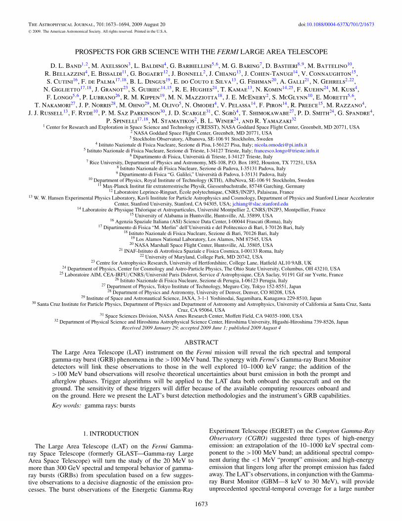
Figure 1. Simulated GRB spectra, showing the broad energy range covered byFermi: (from left to right) the GBM Na i (blue band: 8–2000 keV), the GBMBGO (green: 150 keV–30 MeV) and the LAT (red: 20 MeV to >300 GeV)detectors. The dashed curves are simple extrapolations of the typical GRB 10–1000 keV spectra into the GeV band, while the solid curves add an exponentialcutoff that might result from absorption internal or external to the burst. The twodifferent high-energy photon indices β = −2.25 (black curves) and β = −2.5(gray curves) demonstrate the dependence of the expected LAT flux on thisphoton index. There may be additional high-energy components that are notknown yet and are not shown in the figure.

of bursts. The spectra from these two instruments will coverseven and a half energy decades (<10 keV to >300 GeV; seeFigure 1, which shows different theoretically predicted spec-tra). Thus the LAT will explore the rich phenomena suggestedby the EGRET observations, probing the physical processes inthe extreme radiating regions.

In this paper we provide the scientific community interested inGRBs with an overview of the LAT’s operations and capabilitiesin this research area. Our development of detection and analysistools has been guided by the previous observations and thetheoretical expectations for emission in the >100 MeV band(Section 2). The LAT is described in depth in an instrument paper(Atwood et al. 2009), and therefore here we only provide a briefsummary of the Fermi mission and the LAT, focusing on issuesrelevant to burst detection and analysis (Section 3). Simulationsare the basis of our analysis of the mission’s burst sensitivity,and are largely based on CGRO observations (Section 4). Weuse our simulation methodology to estimate the ultimate burstsensitivity and the resulting burst flux distribution (Section 5).Both the LAT and the GBM will apply burst detection algorithmsonboard and on the ground, and the efficiency of these methodswill determine which bursts the LAT will detect, and with whatlatency (Section 6). Once a burst has been detected, spectraland temporal analysis of LAT (and GBM) data will be possible(Section 7). The burst observations by ground-based telescopesand other space missions, particularly Swift, will complementthe Fermi observations (Section 8). While basic methods are inplace for detecting and analyzing burst data, in-flight experiencewill guide future work (Section 9).

2. BURST PHYSICS ABOVE 100 MeV

2.1. Previous Observations

The detectors of the CGRO provided time-resolved spectra fora statistically well defined burst population. These observations

are the foundation of our expectations for Fermi’s discoveries,which have guided the development of analysis tools beforelaunch.

The Burst And Transient Source Experiment (BATSE) on theCGRO observed a large sample of bursts in the ∼25–2000 keVband with well understood population statistics (Paciesas et al.1999). Spectroscopy by the BATSE detectors found that theemission in this energy band could be described by the empiricalfour-parameter “Band” function (Band et al. 1993)

NBand(E|N0, Ep, α, β) =

× N0

{Eα exp[−E(2 + α)/Ep], E � α−β

2+αEp

Eβ[

α−β

2+αEp

](α−β)exp[β − α],E >

α−β

2+αEp,

(1)

where α and β are the low- and high-energy photon indices,respectively, and Ep is the “peak energy” which corresponds tothe maximum of E2N (E) ∝ νfν for the low-energy component.Typically α ∼ −0.5 to −1 and β is less than −2 (Bandet al. 1993; Preece et al. 2000; Kaneko et al. 2006); the totalenergy would be infinite if β � −2 unless the spectrum hasa high-energy cutoff. The observations of 37 bursts by theCompton Telescope (COMPTEL) on the CGRO (0.75–30 MeV)are consistent with the BATSE observations of this spectralcomponent (Hoover et al. 2005). Because of the relativelypoor spectral resolution of the BATSE detectors (Briggs 1999),this functional form usually is a good description of spectraaccumulated over both short time periods and entire bursts,even though bursts show strong spectral evolution (Ford et al.1995). It is this 10–1000 keV “prompt” component that is wellcharacterized and therefore provides a basis for quantitativepredictions. A detailed duration-integrated spectral analysis (in30 keV-200 MeV) of the prompt emission for 15 bright BATSEGRB performed by Kaneko et al. (2008) confirmed that only infew cases there is a significant high-energy excess with respectto low-energy spectral extrapolations.

The burst observations by the EGRET on the CGRO (20 MeVto 30 GeV) provide the best prediction of the LAT observations.The EGRET observed different types of high-energy burstphenomena. Four bursts had simultaneous emission in both theEGRET and BATSE energy bands, suggesting that the spectrumobserved by the BATSE extrapolates to the EGRET energy band(Dingus 2003). However, the correlation with the prompt phasepulses was hampered by the severe EGRET spark chamberdead time (∼100 ms/event) that was comparable or longerthan the pulse timescales. The EGRET observations of thesebursts suggest that the ∼1 GeV emission often lasts longerthan the lower energy emission, and thus results in part from adifferent physical origin. A similar behavior is present also inGRB 080514B detected by AGILE (Giuliani et al. 2008).

Whether high-energy emission is present in both long andshort bursts is unknown. The four bursts with high-energyemission detected by the EGRET were all long bursts, althoughGRB 930131 is an interesting case. It was detected by theBATSE (Kouveliotou et al. 1994) with duration of T90 =14 s33 and found to have high-energy (>30 MeV) photonsaccompanying the prompt phase and possibly extending beyond(Sommer et al. 1994). The BATSE light curve is dominated bya hard initial emission lasting 1 s and followed by a smoothextended emission. This burst may, therefore, have been one ofthose long bursts possibly associated with a merger and not acollapsar origin, commonly understood as the most probable

33 T90 is the time over which 90% of the emission occurs in a specific energyband.

No. 2, 2009 PROSPECTS FOR GRB SCIENCE WITH THE FERMI LARGE AREA TELESCOPE 1675

origin for short and long burst respectively (Zhang 2007).Several events have now been identified that could fit intothis category (Norris & Bonnell 2006) and their origin is stilluncertain. The LAT will make an important contribution indetermining the nature of the high-energy emission from similarevents and a larger sample of bursts with detected high-energyemission will determine whether the absence of high-energyemission differentiates short from long bursts.

A high-energy temporally resolved spectral component inaddition to the Band function is clearly present in GRB 941017(Gonzalez et al. 2003); this component is harder than the low-energy prompt component, and continues after the low-energycomponent fades into the background. The time integratedspectra of both GRB 941017 and GRB 980923 show thisadditional spectral component (Kaneko et al. 2008).

Finally, the >1 GeV emission lingered for 90 minutes afterthe prompt low-energy emission for GRB 940217, including an18 GeV photon 1.5 hr after the burst trigger (Hurley et al. 1994).Whether this emission is physically associated with the lowerenergy afterglows is unknown.

These three empirical types of high-energy emission—anextrapolation of the low-energy spectra, an additional spectralcomponent during the low-energy prompt emission, and anafterglow—guide us in evaluating Fermi’s burst observationcapabilities.

Because the prompt low-energy component was characterizedquantitatively by the BATSE observations while the EGRET ob-servations merely demonstrated that different components werepresent, our simulations are based primarily on extrapolationsof the prompt low-energy component from the BATSE band tothe >100 MeV band. We recognize that the LAT will probablydetect additional spectral and temporal components, or spectralcutoffs, that are not treated in this extrapolation.

During the first few months of the Fermi mission, theLAT detected already emission from three GRBs: 080825C(Bouvier et al. 2008), 080916C (Tajima et al. 2008) and081024B (Omodei 2008). The rich phenomenology of high-energy emission is confirmed in these three events, wherespectral measurements over various orders of magnitude werepossible together with the detection of extended emission andspectral lags. In particular, GRB 080916C was bright enoughto afford unprecedented broadband spectral coverage in fourdistinct time intervals (Abdo et al. 2009), thereby offering newinsights into the character of energetic bursts.

2.2. Theoretical Expectations

In the current standard scenario, the burst emission arisesin a highly relativistic, unsteady outflow. Several differentprogenitor types could create this outflow, but the initial highoptical depth within the outflow obscures the progenitor type.As this outflow gradually becomes optically thin, dissipationprocesses within the outflow, as well as interactions with thesurrounding medium, cause particles to be accelerated to highenergies and loose some of their energy into radiation. Magneticfields at the emission site can be strong and may be causedby a frozen-in component carried out by the outflow from theprogenitor, or may be built up by turbulence or collisionlessshocks. The emitted spectral distribution then depends on thedetails of the radiation mechanism, particle acceleration, andthe dynamics of the explosion itself.

“Internal shocks” result when a faster region catches up witha slower region within the outflow. “External shocks” occur atthe interface between the outflow and the ambient medium, and

include a long-lived forward shock that is driven into the externalmedium and a short-lived reverse shock (RS) that decelerates theoutflow. Thus the simple model of a one-dimensional relativisticoutflow leads to a multiplicity of shock fronts, and many possibleinteracting emission regions.

As a result of the limited energy ranges of past and currentexperiments, most theories have not been clearly and unam-biguously tested. Fermi’s GBM and LAT will provide an energyrange broad enough to distinguish between different origins ofthe emission; in particular, the unprecedented high-energy spec-tral coverage will constrain the total energy budget and radiativeefficiency, as potentially most of the energy may be radiated inthe LAT range. The relations between the high- and low-energyspectral components can probe both the emission mechanismand the physical conditions in the emission region. The shapeof the high-energy spectral energy distribution will be crucial todiscriminate between hadronic cascades and leptonic emission.The spectral breaks at high energy will constrain the Lorentzfactor of the emitting region. Previously undetected emissioncomponents might be present in the light curves such as thermalemission. Finally, temporal analysis of the high-energy delayedcomponent will clarify the nature of the flares seen in the X-rayafterglows.

2.2.1. Leptonic Versus Hadronic Emission Models

It is very probable that particles are accelerated to very highenergies close to the emission site in GRBs. This could eitherbe in shock fronts, where the Fermi mechanism or other plasmainstabilities can act, or in magnetic reconnection sites. Twomajor classes of models—synchrotron and inverse Comptonemission by relativistic electrons and protons, and hadroniccascades—have been proposed for the conversion of particleenergy into observed photon radiation.

In the leptonic models, synchrotron emission by relativisticelectrons can explain the 10 keV–1 MeV spectrum in ∼2/3 ofbursts (e.g., see Preece et al. 1998), and inverse Compton (IC)scattering of low-energy seed photons generally results in GeVband emission. These processes could operate in both internaland external shock regions (see, e.g., Zhang & Meszaros 2001),with the relativistic electrons in one region scattering the “soft”photons from another region (Fragile et al. 2004; Fan et al.2005; Meszaros et al. 1994; Waxman 1997; Panaitescu et al.1998). Correlated high- and low-energy emission is expected ifthe same electrons radiate synchrotron photons and IC scattersoft photons. In synchrotron self-Compton (SSC) models theelectrons’ synchrotron photons are the soft photons and thusthe high- and low-energy components should have correlatedvariability (Guetta & Granot 2003; Galli & Guetta 2008).However, SSC models tend to generate a broad νFν peak inthe MeV band, and for bursts observed by CGRO this breadthhas difficulty accommodating the observed spectra (Baring &Braby 2004). Fermi, with its broad spectral coverage enabledby the GBM and the LAT, is ideally suited for probing this issuefurther.

Alternatively, photospheric thermal emission might dominatethe soft keV–MeV range during the early part of the promptphase (Rees & Meszaros 2005; Ryde 2004, 2005). Such acomponent is expected when the outflow becomes opticallythin, and would explain low energy spectra that are too hardfor conventional synchrotron models (Crider et al. 1997; Preeceet al. 1998, 2002). An additional power-law component mightunderlie this thermal component and extend to high energy; thiscomponent might be synchrotron emission or IC scattering of


the thermal photons by relativistic electrons. Fits of the sumof thermal and power-law models to BATSE spectra have beensuccessful (Ryde 2004, 2005), but joint fits of spectra from thetwo types of GBM detectors and the LAT should resolve whethera thermal component is present (Battelino et al. 2007a, 2007b).

In hadronic models relativistic protons scatter inelasticallyoff the ∼100 keV burst photons (pγ interactions) producing(among other possible products) high-energy, neutral pions (π0)that decay, resulting in gamma rays and electrons that then radi-ate additional gamma rays. Similarly, if neutrons in the outflowdecouple from protons, inelastic collisions between neutronsand protons can produce pions and subsequent high-energyemission (Derishev et al. 2000; Bahcall & Meszaros 2000).High-energy neutrinos that may be observable are also emittedin these interactions (Waxman & Bahcall 1997). Many vari-ants of hadronic cascade models have been proposed: high-energy emission from proton–neutron inelastic collisions earlyin the evolution of the fireball (Bahcall & Meszaros 2000);proton-synchrotron and photo-meson cascade emission in inter-nal shocks (e.g., Totani 1998; Zhang & Meszaros 2001; Fragileet al. 2004; Gupta & Zhang 2007); and proton synchrotron emis-sion in external shocks (Bottcher & Dermer 1998). A hadronicmodel has been invoked to explain the additional spectral com-ponent observed in GRB 941017 (Dermer & Atoyan 2004).The emission in these models is predicted to peak in the MeVto GeV band (Bottcher & Dermer 1998; Gupta & Zhang 2007),and thus would produce a clear signal in the LAT’s energy band.However, photon–meson interactions would result from a ra-diatively inefficient fireball (Gupta & Zhang 2007), which isin contrast with the high radiative efficiency that is suggestedby Swift observations (Nousek et al. 2006; Granot et al. 2006).Thus, the hadronic mechanisms for gamma-ray production aremany, but the Fermi measurements of the temporal evolution ofthe highest energy photons will provide strong constraints onthese models, and moreover discern the existence or otherwiseof distinct GeV-band components.

2.2.2. High-energy Absorption

At high energies the outflow itself can become opticallythick to photon–photon pair production, causing a break inthe spectrum. Signatures of internal absorption will constrainthe bulk Lorentz factor and adiabatic/radiative behavior of theGRB blast wave as a function of time (Baring & Harding 1997;Lithwick & Sari 2001; Guetta & Granot 2003; Baring 2006;Granot et al. 2008). Since the outflow might not be steady andmay evolve during a burst, the breaks should be time variable,a distinctive property of internal attenuation. Moreover, if theattenuated photons and their hard X-ray/soft gamma-ray targetphotons originate from proximate regions in the bursts, theturnovers will approximate broken power laws. Interestingly,the LAT has already provided palpable new advances in termsof constraining bulk motion in bursts. For GRB 080916C,the absence of observable attenuation turnovers up to around13 GeV suggests that the bulk Lorentz factor may be well inexcess of 500–800 (Abdo et al. 2009).

Spectral cutoffs produced by internal absorption must be dis-tinguished observationally from cutoffs caused by interactionswith the extragalactic background. The optical depth of the uni-verse to high-energy gamma rays resulting from pair produc-tion on infrared and optical diffuse extragalactic backgroundradiation can be considerable, thereby preventing the radiationfrom reaching us. These intervening background fields necessar-ily generate quasi-exponential turnovers familiar to TeV blazar

studies, which may well be discernible from those resultingfrom internal absorption. Furthermore, their turnover energiesshould not vary with time throughout the burst, another distinc-tion between the two origins for pair attenuation. In addition,the turnover energy for external absorption is expected above afew tens of GeV while for internal absorption it may be as lowas � 1 GeV (Granot et al. 2008). Although the external absorp-tion may complicate the study of internal absorption, studies ofthe cutoff as a function of redshift can measure the universe’soptical energy emission out to the Population III epoch (withredshift > 7; de Jager & Stecker 2002; Coppi & Aharonian1997; Kashlinsky 2005; Bromm & Loeb 2006).

2.2.3. Delayed GeV Emission

The observations of GRB 940217 (Hurley et al. 1994) demon-strated the existence of GeV-band emission long after the∼100 keV “prompt” phase in at least some bursts. With themultiplicity of shock fronts and with synchrotron and IC com-ponents emitted at each front, many models for this linger-ing high-energy emission are possible. In combination with theprompt emission observations and afterglow observations bySwift and ground-based telescopes, the LAT observations maydetect spectral and temporal signatures to distinguish betweenthe different models.

These models include: SSC emission in late internal shocks(LIS; Zhang & Meszaros 2002; Wang et al. 2006; Fan et al.2008; Galli & Guetta 2008); external IC (EIC) scattering of LISphotons by the forward shock electrons that radiate the afterglow(Wang et al. 2006); IC emission in the external RS (Wang et al.2001; Granot & Guetta 2003; Kobayashi et al. 2007); and SSCemission in forward external shocks (Meszaros & Rees 1994;Dermer et al. 2000; Zhang & Meszaros 2001; Dermer 2008;Galli & Piro 2007).

A high-energy IC component may be delayed and havebroader time structures relative to lower energy components be-cause the scattering may occur in a different region from wherethe soft photons are emitted (Wang et al. 2006). The correlationof GeV emission with X-ray afterglow flares observed by Swiftwould be a diagnostic for different models (Wang et al. 2006;Galli & Piro 2007; Galli & Guetta 2008).

2.3. Timing Analysis

The LAT’s low deadtime and large effective area will permita detailed study of the high-energy GRB light curve, which wasimpossible with the EGRET data as a result of the large deadtimethat was comparable to typical widths of the peaks in the lightcurve. These measures are clearly important for determiningthe emission region size and the Lorentz factor in the emittingfireball.

The light curves of GRBs are frequently complex and diverse.Individual pulses display a hard-to-soft evolution, with Epdecreasing exponentially with the burst flux. One method ofclassifying bursts is to examine the spectral lag, which relates tothe delay in the arrival of high-energy and low-energy photons(e.g., Norris et al. 2000; Foley et al. 2008). A positive lag valueindicates hard-to-soft evolution (Kocevski & Liang 2003; Hafizi& Mochkovitch 2007), i.e., high-energy emission arrives earlierthan low-energy emission. This lag is a direct consequenceof the spectral evolution of the burst as Ep decays with time.The distributions of spectral lags of short and long GRBs arenoticeably different, with the lags of short GRBs concentratedin the range ± 30 ms (e.g., Norris & Bonnell 2006; Yi et al.2006), while long GRBs have lags covering a wide range with


a typical value of 100 ms (e.g., Hakkila et al. 2007). Stamatikoset al. (2008b) study the spectral lags in the Swift data.

An anti-correlation has been discovered between the lag andthe peak luminosity of the GRB at energies ∼ 100 keV (Norriset al. 2000), using six BATSE bursts with definitive redshift.Brighter long GRBs tend to have a high-peak luminosity andshort lag, while weaker GRBs tend to have lower luminositiesand longer lags. This “lag–luminosity relation” has been con-firmed by using a number of Swift GRBs with known redshift(e.g., GRB 060218, with a lag greater than 100 s; Liang et al.2006). Fermi will be able to determine if this relation extendsto MeV-GeV energies.

A subpopulation of local, faint, long lag GRBs has beenproposed by Norris (2002) from a study of BATSE bursts, whichimplies that events with low-peak fluxes (FP (50–300 keV) ∼0.25 ph cm−2 s−1) should be predominantly long lag GRBs.Norris (2002) successfully tested a prediction that these long lagevents are relatively nearby and show some spatial anisotropy,and found a concentration towards the local supergalacticplane. This has been confirmed with the GRBs observed byINTEGRAL (Foley et al. 2008) where it was found that > 90%of the weak GRBs with a lag > 0.75 s were concentrated in thesupergalactic plane.34 Fermi measures of long lag GRBs willconfirm this hypothesis. An underluminous abundant populationis inferred from observations of nearby bursts associated withsupernovae (Soderberg et al. 2006).

Moreover, some quantum gravity (QG) theories predict anenergy-dependent speed of light (see, e.g., Mattingly 2005),which is often parameterized as

v = c(1 − (

E(z)/Eqg

))(2)

where E(z) is the photon energy at a given redshift, E(z) =Eobs(1 + z), and Eqg is the QG scale, which may be of order∼ 1019 GeV. This energy dependence can be measured fromthe difference in the arrival times of different-energy photonsthat were emitted at the same time; measurements thus far giveEqg greater than a few times 1017 GeV. Such photons might beemitted in sharp burst pulses (Amelino-Camelia et al. 1998);measurements have been attempted (Schaefer 1999; Boggset al. 2004). The most difficult roadblock to reliable quantumgravity detections or upper limits results from the difficulty indiscriminating against time delays inherent in the emission atthe site of the GRB itself, and known to exist from previousobservations. This problem can be addressed by studying asample of bursts at different redshifts, or otherwise calibratingthis effect (Ellis et al. 2006, 2008).

With the energy difference between the GBM’s low-energyend and the LAT’s high-energy end, the good event timing byboth the GBM and the LAT, and the LAT’s sensitivity to high-energy photons, the Fermi mission will place interesting limitson Eqg.

3. DESCRIPTION OF THE FERMI MISSION

3.1. Mission Overview

Fermi was launched on 2008 June 11 into a 96.5 min circularorbit 565 km above the Earth with an inclination of 25.◦6to the Earth’s equator. During the South Atlantic Anomalypassages (approximately 17% of the time, on average) theFermi detectors do not take scientific data. In Fermi’s default

34 A possible counterargument has been recently claimed by Xiao & Schaefer(2009).

observing mode the LAT’s pointing is offset 35◦ from the zenithdirection perpendicular to the orbital plane; the pointing willbe rocked from one side of the orbital plane to the other onceper orbit. This observing pattern results in fairly uniform LATsky exposure over two orbits; the uniformity is increased by the54 d precession of the orbital plane.

The mission’s telemetry is downlinked 6–8 times per dayon the Ku band through the Tracking and Data Relay SatelliteSystem (TDRSS).35 The time between these downlinks, thetransmission time through TDRSS, and the processing at theLAT Instrument Science and Operations Center (LISOC) resultin a latency of 6 hr between an observation and the availabilityof the resulting LAT data for astrophysical analysis. In addition,when burst detection software for either detector triggers,messages are sent to the ground through TDRSS with a ∼15 slatency. The mission’s burst operations are described in greaterdetail below.

3.2. The Large Area Telescope

A product of an international collaboration between NASA,DOE, and many scientific institutions across France, Italy,Japan, and Sweden, the LAT is a pair conversion telescopedesigned to cover the energy band from 20 MeV to greater than300 GeV. The LAT is described in greater depth in Atwoodet al. (2009) and here we summarize salient features usefulfor understanding the detector’s burst capabilities. The LATconsists of an array of 4 × 4 modules, each including a tracker-converter based on silicon strip detector (SSD) technology anda 8.5 radiation lengths Cs i hodoscopic calorimeter. High-energy incoming gamma rays convert into electron–positronpairs in one of the tungsten layers that are interleaved withthe SSD planes; the pairs are then tracked to point back tothe original photons’ direction and their energy is measured bythe calorimeter. A segmented anti-coincident shield surroundingthe whole detector ensures the necessary background rejectionpower against charged particles, whose flux outnumbers that ofgamma rays by several orders of magnitude, and reduce the datavolume to fit in the telemetry bandwidth.

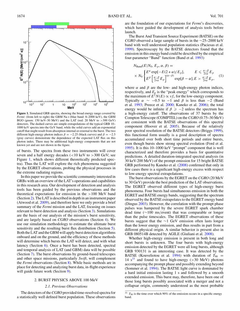
The key points of the LAT design are: wide field of view(FOV—more than 2 sr), large effective area and excellent point-spread function (PSF—see Figure 2), short dead time (∼ 25 μsper event), and good energy resolution (of the order of 10% inthe central region of the active energy range). As a result, theLAT is the most sensitive high-energy gamma-ray detector everflown. The study of GRBs will take particular advantage of theimprovement in angular resolution—we estimate that two orthree photons above 1 GeV will localize a bursts to ∼ 5 arcmin.The reduced dead time will allow the study of the substructure ofthe GRB pulses, typically of the order of milliseconds (Walkeret al. 2000), with a time resolution that has never before beenaccessible at GeV energies.

The data telemetered to the ground consist of the signalsfrom different parts of the LAT; from these signals the groundsoftware must “reconstruct” the events and filter out eventsthat are unlikely to be gamma rays. Therefore, the InstrumentResponse Functions (IRFs) depend not only on the hardware butalso on the reconstruction and event selection software. For thesame set of reconstructed events trade-offs in the event selectionbetween retaining gamma rays and rejecting background resultin different event classes. There are currently three standard

35 See http://msl.jpl.nasa.gov/Programs/tdrss.html.

http://msl.jpl.nasa.gov/Programs/tdrss.html


Energy [MeV]

210

310

410

510

68

%C

on

tain

men

tan

gle

[deg

]

-110

1

10

Energy [MeV]

210

310

410

510

]2

Eff

ecti

ve

Are

a[c

m

2000

4000

6000

8000

10000

12000

Figure 2. Left: comparison of the estimated PSF for the onboard and on-ground event reconstruction and selection. The black solid curve is the 68% containment angleon-axis for the transient event class, while the dashed curve represents the performance of the onboard reconstruction. Right: comparison of the estimated onboard(dashed) and on-ground (solid black curve) on-axis effective areas. These estimates of the instrument response are based on simulations of the LAT.

event classes—the transient, source and diffuse event classes—that are appropriate for different scientific analyses (as theirnames suggest). Less severe cuts increase the photon signal(and hence the effective area) at the expense of an increase inthe non-photon background and a degradation of the PSF andthe energy resolution.

The least restrictive class, the transient event class, is designedfor bright, transitory sources that are not background limited.We expect that the on-ground event rate over the whole FOVabove 100 MeV will be 2 Hz for the transient class and0.4 Hz for the source class. In both cases we expect about onenon-burst event per minute within the area of the PSF aroundthe burst position. Consequently, there should be essentially nobackground during the prompt emission (with a typical durationof less than a minute) so that the transient class is the mostappropriate–and in fact is the one used for producing all theresults presented in this paper. On the other hand, the analysisof afterglows, which may linger for a few hours, will needto account for the non-burst background, at least in the lowregion of the energy spectrum, where the PSF is larger (seeFigure 2).

The onboard flight software also performs event reconstruc-tions for the burst trigger. Because of the available computerresources, the onboard event selection is not as discriminatingas the on-ground event selection, and therefore the onboard bursttrigger is not as sensitive because the astrophysical photons arediluted by a larger background flux. Similarly, larger localiza-tion uncertainties result from the larger onboard PSF, as shownby the left-hand panel of Figure 2.

3.3. Fermi Gamma-ray Burst Monitor

The GBM detects and localizes bursts, and extends Fermi’sburst spectral sensitivity to the energy range between 8 keV and30 MeV or more. It consists of 12 Na i(Tl) (8–1000 keV) and2 BGO (0.15–> 30 MeV) crystals read by photomultipliers,arrayed with different orientations around the spacecraft. TheGBM monitors more than 8 sr of the sky, including the LAT’sFOV, and localizes bursts with an accuracy of < 15◦ (1σ )onboard, (< 3◦ on ground), by comparing the rates in differentdetectors. The GBM is described in greater detail in Meeganet al. (2009).

3.4. Fermi’s Burst Operations

Both the GBM and the LAT have burst triggers. When eitherinstrument triggers, a notice is sent to the ground through theTDRSS within ∼ 15 s after the burst was detected and thendisseminated by the Gamma-ray burst Coordinates Network(GCN)36 to observatories around the world. This initial noticeis followed by messages with localizations calculated by theflight software of each detector. Additional data (e.g., burst andbackground rates) are also sent down by the GBM throughTDRSS for an improved rapid localization on the ground by adedicated processor.

Updated positions are calculated from the full data sets fromeach detector that are downlinked with a latency of a few hours.Scientists from both instrument teams analyze these data, andif warranted by the results, confer. Conclusions from theseanalyses are disseminated through GCN Circulars, free-formattext that is e-mailed to scientists who have subscribed to thisservice. Both Notices and Circulars are posted on the GCNwebsite.

If the observed burst fluxes in either detector exceed pre-setthresholds (which are higher for bursts detected by the GBMoutside the LAT’s FOV), the FSW sends a request that thespacecraft slew to point the LAT at the burst location for afollow-up pointed observation; currently a 5 hr observation isplanned.

In addition to the search for GRB onboard the LAT andmanual follow-up analysis by duty scientists, there is alsoautomated processing of the full science data. This processingperforms an independent search for transient events in the LATdata, to greater sensitivity than is possible onboard, and alsoperforms a counterpart search for all GRB detected within theLAT FoV. This is described in greater detail in Section 6.3.

4. BURST SIMULATIONS

We test the Fermi burst detection and analysis softwarewith simulated data. These simulated data are based on ourexpectations for burst emission in the LAT and GBM spec-tral bands (see Section 2), and on models of the instrumentresponse of these two detectors. Since bursts undoubtedly

36 See http://gcn.gsfc.nasa.gov/.

http://gcn.gsfc.nasa.gov/


Time-Trigger0 10 20 30 40 50 60

GB

MR

ate

[Hz]

0

200

400

600

800

1000

1200

1400

1600

1800

2000

2200

LA

TC

ou

nts

0

1

2

3

4

5

6

71BGO

5NaI

6NaI

LAT

Figure 3. Simulated count rate light curve for a BGO detector, two Na i detectors, and the LAT for one simulated burst. In this model of the burst spectral evolution,the LAT detects counts at the beginning of each pulse; the correlation of the LAT and GBM light curves will be a powerful diagnostic of the emission processes. Thesimulation predicts that the LAT would detect a total of 42 gamma rays above 30 MeV in this moderately bright burst of 1 s peak flux of 63.37 ph cm−2 s−1 between30 and 500 keV.

differ from our theoretical expectations, our calculations aremore reliable in showing the mission’s sensitivity to specificbursts than in estimating the number of bursts that will bedetected.

We have two “GRB simulators” that model the burst flux inci-dent on each detector (Battelino et al. 2007a). The primary is thephenomenological simulator—described in greater detail belowin Section 4.1—that draws burst parameters from observed dis-tributions. We have also created a physical simulator (Omodei2005; Omodei & Norris 2007; Omodei et al. 2007) that calcu-lates the synchrotron emission from the collision of shells in arelativistic outflow (the internal shock model; Piran 1999). Fora given analysis we assemble an ensemble of simulated burstsusing one of these GRB simulators. To simulate a LAT observa-tion of each burst in this ensemble we create a realization of thephoton flux, resulting in a list of simulated photons incident onthe LAT. The LAT’s response to this photon flux is processed inone of two software paths. The first uses “GLEAM,” which per-forms a Monte Carlo simulation of the propagation of the photonand its resulting particle shower in the LAT (using the GEANT4toolkit; Agostinelli et al. 2003) and the detection of particlesin the different LAT components (Atwood et al. 2004; Baldiniet al. 2006). The photon is then “reconstructed” from this sim-ulated instrument response by the same software that processesreal data. Thus GLEAM maps the incident photons into ob-served events. Our second, faster, processing pathway uses theinstrument response functions to map the photons into events di-rectly. We note that both approaches use the same input–a list ofincident photons—and result in the same output—a list of “ob-served” events in one of the event classes. In both approachesGRBs can be combined with other source types (such as station-ary and flaring active galactic nuclei, solar flares, supernova rem-nants, pulsars) to build a very complex model of the gamma-raysky.

The GRB simulators also provide the input to the GBMsimulation software. In this case the GRB simulators produce atime series of spectral parameters (usually the parameters for the“Band” function (Band 2003) discussed above in Section 2.1).The GBM simulation software samples the burst spectrum tocreate a list of incident photons and then uses a model of theGBM response to determine whether each photon is “detected,”and if so, in which energy channel (simulating the GBM’sfinite spectral resolution). Based on a model from the BATSEobservations, background counts are added to the burst counts.

The GBM simulation software outputs count lists, responsematrices, and background spectra in the standard FITS formatsused by software such as XSPEC.37

Because the GRB simulators provide input to both LATand GBM simulations, simulated LAT and GBM data can beproduced for the same bursts, allowing joint analyses. The Fermimission developed the “standard analysis environment” (SAE)to analyze both LAT and GBM data. Data can be binned intime, resulting in light curves (see, for example, Figure 3), or inspectra that can be analyzed using a tool such as XSPEC. As willbe described in Section 7, joint fits of GBM and LAT data maycover an energy band larger than seven orders of magnitude(see Figure 1). Consequently, Fermi will be a very powerfultool for understanding the correlation between low-energy andhigh-energy GRB spectra.

4.1. Phenomenological Burst Model

The phenomenological GRB simulator that is used for mostof our simulations draws from observed spectral and temporaldistributions to construct model GRBs. This modeling assumesthat bursts consist of a series of pulses that can be described bya universal family of functions (Norris et al. 1996)

I (t) = A

{exp[−(|t − t0|/σr )ν], t � t0

exp[−(|t − t0|/σd )ν], t > t0

(3)

where σr and σd parameterize the rise and decay timescale, andν provides the “peakiness” of the pulse. Although empiricallyσr ∼ 0.33σ 0.86

d , we approximate this relation as σr ∼ σd/3. Thepulse full width at half maximum (FWHM) is

W = (σr + σd ) ln(2)1/ν . (4)

Pulses are observed to narrow at higher energy in the BATSEenergy band (Davis et al. 1994; Norris et al. 1996; Fenimoreet al. 1995). Although the statistics in the EGRET data wereinsufficient to determine whether this narrowing continues inthe >100 MeV band, our phenomenological model assumesthat it does. We assume that the FWHM energy dependence isW (E) ∝ E−ξ where ξ is ∼0.4 (Fenimore et al. 1995; Norris

37 See http://heasarc.nasa.gov/xanadu/xspec/.

http://heasarc.nasa.gov/xanadu/xspec/


et al. 1996). Thus, we give the pulse shape in Equation (3) anenergy dependence by setting⎧⎨

⎩σd (E) = 0.75 × ln(2)−1/νW0(E/20 keV)−ξ

σr (E) = 0.25 × ln(2)−1/νW0(E/20 keV)−ξ ,

(5)

where W0 is the FWHM at 20 keV. Burst spectra in the 10–1000 keV band are well described by the “Band” function (Bandet al. 1993) parameterized in Equation (1). Empirically the Bandfunction is an adequate description of burst spectra accumulatedon short timescales (e.g., shorter than a pulse width) and overan entire burst. This may be due in part to the poor spectralresolution of scintillation detectors (such as BATSE and theGBM), but we will treat this as a physical characteristic ofGRBs. In the resulting model, the flux f(t, E) is a product of aBand function with spectral indices α′ and β ′ and the energy-dependent pulse shape I(t, E) (Equation (3) with Equation (5))

f (t, E) = I (t, E)NBand(E|N0, Ep, α′, β ′)ph cm−2 s−1 keV−1.(6)

Note that this spectrum is not strictly a Band function becausethe pulse shape function does not have a power-law energydependence.

The spectrum integrated over the entire burst is a Band func-tion that is proportional to the product W (E)NBand(E|N0, Ep, α′,β ′). Because W (E) is a power law with spectral index −ξ , thespectral indices α and β for the integrated spectrum are differentfrom the indices for the instantaneous flux (Equation (6))∫ ∞

−∞f (t, E)dt = NBand(E|N0, Ep, α, β)T

= A0NBand(E|N0, Ep, α′, β ′)W (E)

= A0W0NBand(E|N0, Ep, α′ − ξ, β ′ − ξ ) (7)

where T is the burst duration and all the normalizing factorsresulting from the integration are incorporated in A0. Thus theflux for a single GRB is the sum of many pulses of the form

f (t, E) = I (t, E)NBand(E|N0, Ep, α + ξ, β + ξ ). (8)

Drawn from observed burst distributions, the same spectralparameters Ep, α, and β are used for a given simulatedburst. The number of pulses and parameters of each pulse(amplitude, width, and peakedness) are also sampled fromobserved distributions (Norris et al. 1996).

Alternative spectral models have also been simulated; forexample, Battelino et al. (2007a) describe simulations with astrong thermal photospheric component.

5. SEMIANALYTICAL SENSITIVITY ESTIMATES

The design of the LAT detector provides an ultimate burstsensitivity, regardless of whether the detection and analysissoftware achieves this ultimate limit. Thus in this section weestimate the LAT’s burst detection and localization capabili-ties, and the expected flux distribution. The following sectiondescribes the current burst detection algorithms.

5.1. Semianalytical Estimation of the Burst DetectionSensitivity

In this subsection we compute the LAT’s burst detection sen-sitivity using a semianalytical approach based on the likelihood

ratio test (LRT) introduced by Neyman & Pearson (1928). Thistest is applied extensively to photon-counting experiments (Cash1979) and has been used to analyze the gamma-ray data fromCOS-B (Pollock et al. 1981, 1985) and EGRET (Mattox et al.1996). The statistic for this test is the likelihood for the null hy-pothesis for the data divided by the likelihood for the alternativehypothesis, here that burst flux is present. This methodology isthe basis of the likelihood tool that will be used to analyze LATobservations; here we perform a semianalytic calculation for thesimple case of a point source on a uniform background.

In photon-counting experiments, the natural logarithm of thelikelihood for a given model can be written as

ln(L) =∑

photons

ln(Mi) − Npred + constant (9)

where Mi is the predicted photon density at the position and timeof ith observed count, and Npred is the predicted total number ofcounts. We compare the log likelihood for the null hypothesisthat only background counts are present versus the hypothesisthat both burst and background counts are present.

The expected number of counts from a burst flux S(E) is

NS = Tobs

∫ΔΩ

∫ E2

E1

Aeff(E)S(E)F (E, Ω) dEdΩ (10)

while the expected number of counts from a background fluxB(E) (assumed to be uniformly distributed over the sky) is

NB = Tobs

∫ E2

E1

Aeff(E)B(E)dEΔΩ (11)

where Aeff is the effective area and F (E, Ω) is the normalizedPSF (which therefore does not show up in Equation (11)). Notethat B(E) varies significantly over the sky, but our assumptionis that it is constant over ΔΩ.

The logarithm of the likelihood of the null hypothesis is

ln(L0) = Tobs

∫ΔΩ

∫ E2

E1

Aeff(E)[S(E)F (E, Ω) + B(E)]

× ln(Aeff(E)B(E))dEdΩ − NB. (12)

The actual count rate is assumed to result from both backgroundand burst flux while the predicted count rates (the Mi inEquation (9) and the total number of counts Npred) are calculatedonly for the background flux (the null hypothesis).

Similarly, the logarithm of the likelihood of the hypothesisthat a burst is present is

ln(L1) =[Tobs

∫ΔΩ

∫ E2

E1

Aeff(E)[S(E)F (E, Ω) + B(E)]

× ln(Aeff(E)[S(E)F (E, Ω) + B(E)])dEdΩ] − (NS + NB).

(13)

Here both the actual and predicted count rates are calculated forboth burst and background fluxes.

Wilks’ theorem (Wilks 1938) defines the Test Statistic asTS = −2(ln(L0) − ln(L1)), and states that TS is distributed(asymptotically) as a χ2 distribution of m degrees of freedom,where m is the number of burst parameters. From Equations (12)and (13) TS is

TS = 2Tobs

∫ΔΩ

∫ E2

E1

Aeff(E)B(E)[(1 + G(E, Ω))

× ln(1 + G(E, Ω)) − G(E, Ω)]dEdΩ (14)


where we have defined a signal-to-noise ratio G(E, Ω) =S(E)F (E, Ω)/B(E).

The significance of a source detection in standard deviationunits is calculated as Nσ = √

TS in the case m = 1 (χ2 with 1dof). Here we assume that Wilks’ theorem holds, which mightbe not absolutely true in a low-count regime (see, in particular,the discussion in Section 6.5). However, we will see that thismethod gives a robust estimate of the LAT sensitivity to GRBs.We can use this method to estimate the LAT sensitivity to GRB.

In our modeling we assume the burst has a “Band” functionspectrum (see Equation (1)) and that the flux is constant over aduration TGRB. Since we seek the optimal detection sensitivity,we calculate TS for Tobs = TGRB. We assume a spatially uniformbackground with a power-law spectrum

B(E) = B0

(E

100 MeV

)γ

ph cm−2 MeV−1 s−1 sr−1 (15)

where the value of the normalization constant B0 is set to mimicthe expected background rate. For modeling the onboard triggerthe background rate above 100 MeV is set to 120 Hz, while,for the on-ground trigger the background is set to 2 Hz, as willbe discussed below. The spectral index is set to be γ = −2.1.The results depend on the value of the spectral index; a detailedstudy of the dependence of the results as a function of the shapeof the residual background is outside the illustrative goal of thissection, thus we omit such discussion. We require TS � 25 andat least 10 source counts in the LAT detector, correspondingto a threshold significance of 5σ and a minimum number ofGRB counts to see a clear excess in the LAT data even in thecase of very few background events. We use the “transient”event class described in Section 3.2, and compute the minimum50–300 keV fluence of bursts at this detection threshold. Theburst fluxes in the LAT band depend only on the high-energypower-law component of the “Band” spectrum; assumed valuesof the low-energy power-law spectral index α = −1 andEp = 500 keV are used to express the spectrum’s normalizationin familiar fluence units. Results are shown in Figure 4; at shortdurations the threshold is determined by the finite number ofburst photons, while the background determines the thresholdfor longer durations. This figure predicts that unless other high-energy spectral components are present, the bursts detected bythe LAT will be “hard” with photon indices β near −2 (Band2007).

These estimates consider the detectability of individual bursts.We can compute the sensitivity of the LAT detector to GRBconsidering as input the observed distribution of GRB withknown spectral parameters. We use the catalog of bright bursts(Kaneko et al. 2006) to quantify the characteristics of GRBs.This catalog contains 350 bright GRBs over the entire lifeof the BATSE experiment selected for their energy fluence(requiring that the fluence in the 20–2000 keV band is greaterthan 2×10−5 erg cm−2) or on their peak photon flux (over256 ms, in the 50–300 keV, greater than 10 ph cm−2 s−1).This subset of burst of the whole BATSE catalog representsthe most comprehensive study of spectral properties of GRBprompt emission to date and is available electronically from theHigh-Energy Astrophysics Science Archive Research Center(HEASARC).38 We restrict our sample of GRB to the ones witha well reconstructed Epeak; furthermore, we exclude the burstsdescribed by the Comptonized model (COMP) for which an

38 http://heasarc.gsfc.nasa.gov/.

GRB Duration (s)

-210 -110 1 10210

310

)2

Flu

en

ce

[50-3

00

keV

](e

rg/c

m

-910

-810

-710

-610

-510

-410

-310

-210

=-1.0αEp=300,

=-2.00β=-2.25β=-2.50β=-2.75β

Figure 4. Threshold fluence as a function of the GRB duration, for on-grounddetection and for on-axis incidence. Threshold fluence increases by factor of ∼2 for z-axis angles of 50 degrees. Different lines are related to different spectralindex. Also plotted are the observed bursts from the BATSE catalog.

emission at LAT energy is very unlikely; we also reject burstswith spectra described by a single power law with undeterminedEpeak (probably outside the BATSE energy range).

Considering the field of view of the BATSE experiment andthese selection criteria, we estimate a rate of 50 GRB per year(full sky). For each burst we simulate, the duration, the energyfluence, and the spectral parameters are in agreement with oneof the bursts in the Bright BATSE catalog. Its direction israndomly chosen in the sky, and for each burst we computethe LAT response functions for that particular direction. Finally,we compute Ts using Equation (14). The resulting distributionsare given by Figure 5.

The onboard analysis’ larger effective area (Figure 2) resultsin a larger cumulative burst rate, but not a larger detected ratebecause of the larger background rate. Events that are processedonboard by the GRB search algorithm are downloaded, and alooser set of cuts can be chosen on-ground in order to optimizethe signal/noise ratio. We emphasize that this calculation makesa number of simplifying assumptions. The LAT spectrum isassumed to be a simple extrapolation of the spectrum observedby BATSE. Spectral evolution within a burst is not considered.The BATSE burst population was biased by that instrument’sdetection characteristics. Nonetheless we estimate that the LATcan detect around 1 burst per month, with a few bursts per yearhaving more than 100 counts. These few bright bursts are likelyto have a large impact on burst science since detailed spectralanalysis will be possible.

In the framework described in this section, we can alsoestimate the localization accuracy for the burst sample, for bothonboard and on-ground triggers. If σi is the 68% containmentradius for the single photon PSF, then the localization iscomputed as

σ−1GRB =

√∑i

1

σ 2i

(16)

http://heasarc.gsfc.nasa.gov/


Number of LAT counts

1 10210

310 410

Nu

mb

er

of

GR

B/y

r

-110

1

10

Number of LAT counts

1 10210

310 410

Nu

mb

er

of

GR

B/y

r

-110

1

10

Figure 5. Integrated number of GRBs per year as a function of the number of LAT counts. The solid curve shows all bursts in the sample, while the dashed curve givesthe detected bursts. Left panel: on-ground analysis (“transient” class, 2 Hz background rate above 100 MeV). Right panel: onboard analysis (120 Hz background rate).

(A color version of this figure is available in the online journal.)

error radius (degrees)σ1-

-310 -210 -110 1 10

Nu

mb

er

of

LA

Tco

un

ts

1

10

210

310

410

510

error radius (degrees)σ1-

-310 -210 -110 1 10

Nu

mb

er

of

LA

Tco

un

ts

1

10

210

310

410

510

Figure 6. Number of LAT counts vs. localization accuracy. In each panel the red triangles denote detected bursts and the open blue circles show undetected bursts.The left and right panels are for the on-ground and onboard localizations. Thus the on-ground analysis results in a slightly larger burst detection rate and a betterlocalizations. The superior track reconstruction and background reduction outweighs the smaller effective area in increasing the on-ground detection rate.


that, in terms of the previously defined quantities, is

σ−1GRB =

√TGRB

3

∫ E2

E1

Aeff(E)S(E)

σ68%(E)2dE. (17)

The factor of 3 takes into account the non-gaussianity of thePSF, and was estimated by Burnett (2007). We compute thelocalization accuracy for each burst in our sample. Figure 6shows the results. In each plot the detected burst are representedby red triangles, while the blue empty circles are the bursts withLAT counts that did not pass our detection condition.

These results show that the LAT can localize bursts withsubdegree accuracy, both onboard and on-ground. The GRByield is greater and bursts are better-localized on-ground thanonboard. The on-ground analysis is available only after the fulldata set is downlinked and processed. This process can lastsfew hours, depending on the position of the downlink contact.Onboard localization is delivered quasi-real time with onboardalerts. For those bursts, multiwavelength follow-ups will befeasible for bursts localized within a few tens of arcminutes.

For example, the FOV of Swift’s XRT is about 0.◦4 and isof the same order as the FOV of the typical mid-size opticalor near-IR (NIR) telescope. Afterglow searches in the opticaland NIR are very successful–∼60% of the Swift bursts havebeen associated with optical and NIR afterglows. Figure 6shows that a sizeable fraction of Fermi GRB detections willbe localized within these requirements, and relatively largeFOV ground-based observatories (∼30 arcmin) with optical/NIR filters (I, z, J,H,K) should produce a fairly high detectionrate for the afterglows of LAT-detected GRBs.

5.2. Estimated LAT Flux Distribution

We now consider the full GRB model described in Section 4for estimating the expected LAT flux distribution. This is, ofcourse, very dependent on the assumptions of the GRB model,and the final result should be considered only as a prediction ofthe flux distribution.

We use the bright BATSE catalog (Kaneko et al. 2006) forthe burst population, as described in the previous section. In


Duration [s]

-110 1 10

210

Nu

mb

er

of

Sim

ula

ted

Mo

de

l

1

10

Fluence 50-300 keV [erg/cm^2]

-810

-710

-610

-510

-410

Nu

mb

er

of

Sim

ula

ted

Mo

de

l

1

10

210

50-300 keV [1/cm^2/s]256 ms

PeakFlux1 10

210

310

Nu

mb

er

of

Sim

ula

ted

Mo

de

l

1

10

)αLow Energy Spectral Index (

-2 -1.5 -1 -0.5 0 0.5N

um

be

ro

fS

imu

late

dM

od

el

1

10

)p

N(e) Spectrum (E2

Peak of the e

210

310

Nu

mb

er

of

Sim

ula

ted

Mo

de

l

1

10

)βHigh Energy Spectral Index (

-7 -6 -5 -4 -3 -2 -1

Nu

mb

er

of

Sim

ula

ted

Mo

de

l

1

10

210

Figure 7. Parameter distributions for the simulated bursts of the bright burst BATSE catalog (dashed lines). Filled dark histograms represent the GRBs with morethan 1 predicted count above 100 MeV in the LAT detector, while for the light filled histograms we have also required that the high-energy spectral index beta ismore negative than −2. The distributions show the logarithm of the duration, the fluence, the peak flux distribution, the low and high-energy spectral indexes, and thelogarithm of the energy of the peak of the νFν spectrum.

addition, we also select a subsample of bursts for which betais more negative than −2. This is motivated by the fact that apower-law index greater than −2 implies a divergence in thereleased content of energy, thus those value are unphysical anda cutoff should take place. The measurements yielding betagreater than −2 are questionable and suggest either an ill-determined quantity for a true spectrum that is in reality softer,or an additional spectral break above the energies measured withthe BATSE. Given the duration, the number of pulses is fixed bythe total burst duration. Pulses are combined together in orderto obtain a final T90 duration. Correlations between duration,intensity, and spectral parameters are automatically taken intoaccount as each of these bursts corresponds to an entry in theKaneko et al. catalog. The emission is extended up to highenergy with the model described in Section 4.

We emphasize again that this model ignores possible in-trinsic cutoffs (resulting from the high end of the particledistribution or internal opacity; Section 2.2.2), and additionalhigh-energy components suggested by the EGRET observations(Section 2.1). High-energy emission (>10 GeV) is also sensi-

tive to cosmological attenuation due to pair production betweenthe GRB radiation and the extragalactic background light (EBL;Section 2.2.2). The uncertain EBL spectral energy distributionresulting from the absence of high-redshift data provides a va-riety of theoretical models for such diffuse radiation. Thus theobservation of the high-energy cutoff as a function of the GRBdistance can, in principle, constrain the background light. In oursimulation we include this effect, adopting the EBL model inKneiske et al. (2004). Short bursts are thought to be the result ofthe merging of compact objects in binary systems, so we adoptthe short burst redshift distribution from Guetta & Piran (2005),while long bursts are related to the explosive end of massivestars, whose distributions are well traced by the star formationhistory (Porciani & Madau 2001).

In Figure 7 the sampled distributions are shown. The dashedline histogram is obtained from the full bright burst BATSEcatalog. In order to increase the number of burst in the field ofview of the LAT detector we over-sampled the original catalogby a factor 1.4. The dark filled histograms show the distributionof GRB with at least 1 count in the LAT detector, and the


Number Of Photons Detected1 10

2103

10

Nu

mb

er

Of

GR

B/y

r

1

10

>1 GeV

>10 GeV

>100 MeV

>1 GeV

>10 GeV

All selected Burst

Only bursts with Beta<-2

Figure 8. Model-dependent LAT GRB sensitivity. The GRB spectrum isextrapolated from BATSE to LAT energies. The all-sky burst rate is assumedto be 50 GRB yr−1 full sky (above the peak flux in 256 ms of 10 ph s−1 cm−2

in the 50–300 keV or with an energy flux in the 20–2000 keV band greaterthan 2× 10−5 erg cm−2), based on BATSE catalog of bright bursts. The effectof the EBL absorption is included. Different curves refer to different energythresholds. Dashed curves are the result of the analysis excluding very hardbursts, with a beta greater than −2.

light filled histograms are the subsample of detected GRB withbeta < −2.

We simulate approximately 10 years of observations inscanning mode. The orbit of the Fermi satellite, the SouthAtlantic Anomaly (SAA) passages and Earth occultations areall considered. In Figure 8 we plot the number of expectedbursts per year as a function of the number of photons per burstdetected by the LAT. The different couples of lines refer todifferent energy thresholds (100 MeV, 1 GeV, and 10 GeV).Dashed lines are the same computation but using only thesubsample of GRBs with beta more negative than −2 (the lightfilled distribution in Figure 7). The EBL attenuation affects onlythe high-energy curve, as expected from the theory, leaving thesensitivities almost unchanged below 10 GeV. Assuming thatthe emission component observed in the 10–1000 MeV bandcontinues unbroken into the LAT energy band, we estimate thatthe LAT will independently detect approximately 10 bursts peryear, depending on the sensitivity of the detection algorithm;approximately one burst every three months will have morethan a hundred counts in the LAT detector above 100 MeV:these are the bursts for which a detailed spectral or even timeresolved spectral analysis will be possible. If we restrict ouranalysis to the subsample of bursts with beta more negative than−2, these numbers decrease. Nevertheless, even if we adoptthis conservative approach, the LAT should be able to detectindependently approximately 1 burst every two months, andwill be able to detect radiation up to tens of GeV.

With the assumed high-energy emission model a few burstsper year will show high-energy prompt emission, with photonsabove 10 GeV. These rates are in agreement with the number ofbursts detected in the LAT data after few months (GRB080825C(Bouvier et al. 2008), GRB080916C (Tajima et al. 2008),GRB081024B (Omodei 2008)), but the statistics is still lowfor any strong constraint on the burst population.

6. GAMMA-RAY BURST DETECTION

The rapid detection and localization of bursts is a major goalof the Fermi mission. Both Fermi instruments will search for

bursts both onboard and on-ground. These searches will detectbursts on different timescales and with different sensitivities.Here we focus on LAT burst detection, but for completeness wedescribe briefly GBM burst detection.

6.1. GBM Burst Detection

Onboard the Fermi observatory the GBM will use rate triggersthat monitor the count rate from each detector for a statisticallysignificant increase. Similar to the BATSE detectors, the GBMas a whole will trigger when two or more detectors trigger. A ratetrigger compares the number of counts in an energy band ΔEover a time bin Δt to the expected number of background countsin this ΔE–Δt bin; the background is estimated from the ratebefore the time bin being tested. The GBM trigger uses the 12Na i detectors with various energy bands, including ΔE = 50–300 keV, and time bins from 16 ms to 16.384 s. Note thatthe BATSE trigger had one energy band—usually ΔE = 50–300 keV–and the three time bins Δt =0.064, 0.256, and 1.024s. The GBM burst detection algorithms are described in greaterdetail in Meegan et al. (2009).

When the GBM triggers it sends a series of burst alert packetsthrough the spacecraft and TDRSS to the Earth. Some of theseburst packets, including the burst location calculated onboard,will also be sent to the LAT to assist in the LAT’s onboardburst detection. Burst locations are calculated by comparing therates in the different detectors; each the detectors’ effective areavaries across the FOV. In addition, the GBM will send a signalover a dedicated cable to the LAT; this signal will only informthe LAT that the GBM has triggered.

The continuous GBM data that are routinely telemetered tothe ground can also be searched for bursts that did not trigger theGBM onboard. These data will provide rates for all the GBMdetectors in eight energy channels with 0.256 s resolution andin 128 energy channels with 4.096 s resolution. In particular, ifa burst triggers the LAT but not the GBM, these rates will atthe very least provide upper limits on the burst flux in the GBMenergy band.

6.2. Onboard LAT Detection

The LAT flight software will detect bursts, localize them,and report their positions to the ground through the burst alerttelemetry. The rapid notification of ground-based telescopesthrough GCN will result in multi-wavelength afterglow observa-tions of GRBs with known high-energy emission. The onboardburst trigger is described in Kuehn et al. (2007).

The onboard processing that results in the detection of a GRBcan be subdivided into three steps: initial event filtering; eventtrack reconstruction; and finally burst detection and localization.In the first step all events—photons and charged particles—thattrigger the LAT hardware are filtered to remove events thatare of no further scientific interest. The events that survivethis first filtering constitute the science data stream that isdownlinked to the ground for further processing. These eventsare also fed into the second step of the onboard burst processingpathway.

The second step of the burst pathway attempts to reconstructtracks for all the events in the science data stream using the “hits”in the tracker’s silicon strip detectors that indicate the passage ofa charged particle. The burst trigger algorithm uses both spatialand temporal information, and therefore a three-dimensionaltrack that points back to a photon’s origin is required. Tracks canbe calculated for only about a third the events that are input to this


step, although surprisingly the onboard track-finding efficiencyis 80%–90% of the more sophisticated ground calculation.However, the onboard reconstruction is less accurate, resultingin a larger PSF onboard than on-ground, as is shown by Figure 2.A larger fraction of the incident photons survive the onboardfiltering than survive the on-ground processing at the expense ofa much higher non-photon background onboard than on-ground;consequently the onboard effective area is actually larger thanthe on-ground effective area, as Figure 2 shows.

The rate of events that pass the onboard gamma filter(currently the same event set that is downlinked and thusavailable on-ground) is ∼400 Hz. The rate that events are sentto the onboard burst trigger, which requires three-dimensionaltracks, is ∼120 Hz. The on-ground processing creates a transientevent class with a rate of ∼2 Hz. Thus onboard the burst triggermust find a burst signal against a background of ∼120 non-burstevents, while on-ground this background is only ∼2 Hz. Thisdifference in non-burst background rate sets fundamental limitson the onboard and on ground burst detection sensitivities.

The third step in the burst processing is burst detection, whichconsiders the events that have passed all the filters of the firsttwo steps, and thus have arrival times, energies and originson the sky. When a detector such as the GBM provides onlyevent rates, the burst trigger can only be based on a statisticallysignificant increase in these rates. However, when a detectorsuch as the LAT provides both spatial and temporal informationfor each event, an efficient burst trigger will search for temporaland spatial event clustering. Most searches for transients binthe events in time and space (if relevant), but the LAT uses anunbinned method.

The LAT burst trigger searches for statistically significantclusters in time and space. The trigger has two tiers. The firsttier identifies potentially interesting event clusters for furtherinvestigation by the second tier; the threshold for the first tierallows many false tier 1 triggers that are then rejected by thesecond tier. The first tier operates continuously, except while thesecond tier code is running. A GBM trigger is equivalent to afirst tier trigger in that the GBM’s trigger time and position arepassed directly to the second tier.

Tier 1 operates on sets of N events that survived the first twosteps, where currently N is in the range of 40–200. The effectivetime window that is searched is N divided by the event rate; foran event rate of 120 Hz and these values of N, the time windowis 1/3–5/3 s. Each of these N events is considered as the seed fora cluster consisting of all events that are within θ0 of the seed;currently θ0 = 17◦, approximately the 68% containment radiusof the onboard three-dimensional tracks at low event energies. Aclustering statistic, described below, is then calculated for eachcluster. A tier 1 trigger results when a clustering statistic for anycluster exceeds a threshold value. A candidate burst location isthen calculated from the events of the cluster that resulted in thetier 1 trigger.

The onboard burst localization algorithm uses a weightedaverage of the positions of the cluster’s events. The weightingis the inverse of the angular distance of an event from the burstposition. Since the purpose of the algorithm is to find the burstposition, the averaging must be iterated, with the weightingused in one step calculated from the position from the previousstep. The initial location is the unweighted average of the eventspositions. The convergence criterion is a change of 1 arcminbetween iterations (with a maximum of 10 iterations). Theposition uncertainty depends on the number and energies ofevents, but the goal is an uncertainty less that 1◦. Using Monte

Carlo simulations, this methodology was found to be superiorto others that were tried.

The tier 1 trigger time and localization (or if the GBM trig-gered, its trigger time and burst position) are then passed tothe second tier. Because the second tier is run relatively infre-quently, it can consider a much larger set of events than the firsttier. Currently 500 events are considered, which corresponds toa time window of ∼4.2 s. A cluster is then formed from allevents in this set that are within θ2 (∼10◦) of the tier 1 burstlocation. A clustering statistic is then calculated for this cluster,and if its value exceeds a threshold, a tier 2 trigger results and thecluster events are run through the localization algorithm. Theresulting trigger time, burst location and number of counts infour energy bands are then sent to the ground through the burstalert telemetry. The second tier is run repeatedly after a tier 1trigger in case the burst brightens resulting in a larger clustercentered on the tier 1 position, and consequently a tier 2 trigger(if one has not yet occurred) and a better burst localization (if atier 2 trigger does occur).

The clustering statistic is based on the probabilities that thecluster’s events have the observed distances from the clusterseed position and the arrival time separations, under the nullhypothesis that a burst is not occurring. Assuming events arethrown uniformly onto a sphere (the null hypothesis), theprobability ps of finding an event within θ degrees of the clusterseed position is

ps = 1 − cos(θ )

1 − cos(θm)(18)

where it is assumed that there are no events at more thanθm = 115◦ (the performance is not sensitive to this parameter).Thus for a cluster of M events the spatial contribution to theclustering statistic is

PS =M∑i=1

|log10(psi)| =

M∑i=1

∣∣∣∣∣log10

(1 − cos(θi)

1 − cos(θm)

)∣∣∣∣∣ . (19)

The temporal part of the cluster probability assumes thatthe event arrival time follows a Poisson distribution (again thenull hypothesis). The probability that the arrival times of twosubsequent events differ by ΔT is

pt = 1 − exp[−rtΔT ], (20)

where rt is the rate at which events occur within the area ofthe cluster. The temporal contribution of each cluster to theclustering statistic is

PT =M∑i=1

|log10(pti )| =M∑i=1

∣∣∣∣log10(1 − e−rt ΔTi )

∣∣∣∣ . (21)

The trigger criterion is

ξPT + PS > Θ (22)

where ξ is an adjustable parameter that assigns relative weightsto the spatial and temporal clustering, and Θ is the threshold.The two tiers may use different values of both ξ and Θ. Theoverall false trigger rate depends on the tier 2 value of Θ.

The parameters used by the onboard burst detection andlocalization software are sensitive to the actual event rates, andwill ultimately be set based on flight experience. Currently thethresholds are set high enough to preclude any triggers, and


log-probability

Entr

ies

/bin

-120 -80 -40 010

0

101

102

103

104

105

Figure 9. Distribution of log-probability values under the null hypothesisobtained from applying the ground-based version of the GRB search algorithmto sets of 20 counts. The shaded region indicates the range over which a Gaussianfunction, shown in red, was fit to these data. The resulting 5σ threshold at anoverall log-probability value of −117 is plotted as the vertical dashed line. Burstcandidates are required to have log-probabilities below this threshold.


diagnostic data is being downlinked and studied. The thresholdswill eventually be lowered, keeping the false trigger rate at anacceptable level.

Based on preliminary calculations using a burst populationbased on the BATSE, we estimate ∼1 bursts every two monthswill be detected and localized to 1◦ (see Figure 5 and Figure 6).

6.3. LAT Ground-Based Blind Search

A burst detection algorithm will be applied on the ground toall LAT counts after the events are reconstructed and classified todetect bursts that were not detected by the onboard algorithm,the GBM, or other missions and telescopes. Thus this “blindsearch” is similar to the first tier of the onboard burst detectionalgorithm. The ground-based search will be performed aftereach satellite downlink; to capture bursts that straddle thedownlink boundaries, some counts from the previous downlinkare buffered and used in searching for bursts in the data froma given downlink. The ground-based blind search algorithmis very similar to the onboard algorithm described in theprevious section, but will benefit from the full ground-basedevent reconstruction and background rejection techniques thatare applied to produce the LAT counts used for astrophysicalanalysis. For these data, the particle background rates willbe lower than the onboard rates by at least two orders-of-magnitude. Furthermore, the reconstructed photon directionsand energies will be more accurate than the onboard quantities.Figure 2 compares the 68% containment angle as a function ofthe photon energy for the onboard and on-ground LAT countdata sets.

In addition to differing in the reconstruction and backgroundfiltering, the ground-based analysis treats the input data slightlydifferently. The first stage of the ground-based algorithm isapplied to consecutive sets of 20 to 100 counts. As withthe onboard algorithm, the number of counts analyzed isconfigurable and will be adjusted with the growth of ourknowledge of GRB prompt emission in the LAT band and

log_prob_spatial

log

_p

rob

_te

mp

ora

l

Entries/bin

-300 -200 -100 0

-200

-150

-100

-50

0

100

101

102

103

104

Figure 10. Two-dimensional histogram of the spatial and temporal log-probability components. The dashed line indicates the 5σ threshold (an overalllog-probability value of −117) derived from the null distribution (Figure 9).Burst candidates are required to lie below this line.


of the residual instrumental background. However, in contrastto the onboard algorithm, the data sets do not overlap. Thisensures that each segment is statistically independent andgenerally better separates the log-probability distributions ofthe null case (i.e., where there is no burst) from the distributionscomputed when burst photons are present. Figure 9 shows thereference distribution for the null case derived from simulatedbackground data. We modeled the low end (large negativevalues) of the distribution with a Gaussian, and set the burstdetection threshold at 5σ from the fitted peak. Since thisdistribution is derived from pre-launch Monte Carlo simulationswith assumed incident particle distributions and other expectedon-orbit conditions, the thresholds are being re-calibrated withreal flight data. Since we perform an empirical thresholdcalibration, we can neglect the constant normalization factorsin the denominators of the single event probabilities shown inEquations (18) and (20).

The overall log-probability is the sum of spatial and temporalcomponents (see Equation (22)), which we weight equally(ξ = 1). Figure 10 shows the two-dimensional distributionsfor the temporal and spatial components. The dashed line inFigure 10 corresponds to the 5σ threshold with this weighting.Figure 11 shows the time history of the log-probabilities asapplied to the GRB grid data. The excursions across thethreshold line indicate the burst candidates.

While the onboard burst trigger performs two passes throughthe data with the temporal-spatial clustering likelihood algo-rithm, the ground-based detection analysis performs only onesuch pass. If a candidate burst is found in the ground-basedanalysis, counts from a time range bracketing the trigger timeundergoes further processing to determine the significance of theburst. If the burst is sufficiently significant, it is localized andits spectrum is analyzed. These analyses use the unbinned max-imum likelihood method that is applied to LAT point sources.

6.4. GRB Candidate Follow-up Processing

When a candidate burst location and trigger time is providedby the ground-based blind search, a LAT or GBM onboardtrigger, or another burst detector such as Swift—we will call this


Figure 11. Time history of the ground-based log-probability. The horizontaldashed line shows the 5σ threshold derived from the Gaussian function fit tothe log-probabilities distribution under the null hypothesis (Figure 9). Burstcandidates are required to lie below this line.

a first stage detection—a LAT ISOC data processing pipelinewill analyze the LAT counts to determine the significance ofa possible LAT detection. This step in deciding whether theLAT has detected a burst is similar to the tier two analysis ofthe onboard algorithm. If the LAT has detected a burst, thepipeline will localize the burst and determine its temporal startand stop. All of the analyses described in this section will beperformed using the “transient” class. These data selections havea larger effective area at a cost of somewhat higher instrumentalbackground, particularly in the 50–200 MeV range. For brighttransients, such as are expected for GRBs, this trade-off isadvantageous given the short time scales.

The first step in the follow-up processing is determining thetime interval straddling the candidate burst during which theLAT count rate is greater than the expected background rate.The counts are selected from a 15◦ acceptance cone centeredon the candidate burst position and from a 200 s time windowcentered on the candidate burst trigger time. This time windowis designed to capture possible precursor emission that maybe present in the LAT band. Both the acceptance cone radiusand the time window size are configurable parameters in theprocessing pipeline. With this acceptance cone radius, the totalevent rate from non-GRB sources is expected to be < 0.1 to0.5 Hz for normal scanning observations, depending on how farthe candidate position is from the brightest parts of the Galacticplane emission. The event arrival times are analyzed using aBayesian blocks algorithm (Jackson et al. 2003; Scargle 1998)that aggregates arrival times in blocks of constant rate and identi-fies “change points” between blocks with statistically significantchanges in event rate. The burst start and stop time are identifiedas the first and last change points from the resulting light curve.An example of the results of this analysis is shown in Figure 12.

If no change points are found within the 200 s bracketingtime window, then the counts from the first stage time windowand burst position will be used in calculating upper limits.In these cases, the position refinement step will be skippedand background model components will be included in thesignificance and upper limits analysis.

MET - 258063539 (s)

En

trie

s/b

in

-100 -50 0 50 1000

10

20

30

40

Figure 12. LAT counts light curve for a simulated burst (solid histogram) anda piece-wise constant light curve derived using the Bayesian blocks analysis ofthe event arrival times (dashed histogram).

If application of the Bayesian block algorithm to the LATarrival times finds a statistically significant increase in the countrate above background, i.e., if at least two change points werefound, then further analysis uses only the counts between thefirst and last change points to exclude background. The positionis refined with the standard LAT maximum likelihood softwarethat folds a parameterized input source model through theinstrument response functions to obtain a predicted distributionof observed counts. The parameters of the source model areadjusted to maximize the log-likelihood of the data given themodel. For these data, the background counts are sufficientlysmall that a model with the different background componentsusually used in point source analysis is not needed, and a modelwith a single point source should suffice to localize the burst.The burst spectral parameters and burst coordinates are adjustedwithin the extraction region to maximize the log-likelihood,and the best-fit position is thereby obtained. Error contours arederived by mapping the likelihood surface in position space,with 90% confidence limit (CL) uncertainties given by thecontour corresponding to a change in the log-likelihood of 2.305.This value is equal to Δχ2/2 for 2 degrees-of-freedom (dof).Figure 13 shows an example counts map with the 90% CLcontour overlaid.

For spectral analysis and the definitive burst significancecalculation we use the counts within the first and last changepoints and at the center of a 15◦ radius acceptance cone aroundthe maximum likelihood position. Again we use maximumlikelihood to derive the basic burst parameters from the LAT dataalone. Since this is an automated procedure, a simple power-lawmodel is chosen as the default. For brighter bursts, backgroundmodel components are not needed. For fainter bursts, such asthose burst candidates for which we only have a first stagedetection, including the background is essential to determinethe significance of a faint burst in the LAT data and for derivingupper limits.

6.5. Quantifying Significance and Upper Limits

As discussed in Section 5.1, the LRT is a natural frame-work for hypothesis testing, and we will use this method forquantifying the significance of a candidate burst. The back-


Figure 13. LAT counts map for the simulated burst in Figure 12 using only thecounts between the first and last change points. The best-fit position and 90%error contour derived from the maximum likelihood analysis are overlaid. Thecolor scale on the right shows the counts per pixel.


ground models used for the null hypothesis (i.e., that a burst isnot present) can be simplified considering the expected numberof counts from each background component over the short GRBtime scales (< O(102) s). For determining the significance of asource, we compute the test statistic defined in Equation (14).We are fairly conservative and require a Ts > 25, correspondingto 5σ for 1 dof, in order to claim a detection.

Upper limits may be computed in several different ways.A method that has been used in the past for GRBs and othertransient astronomical sources is a variant of the classical “onsource-off source” measurement. In this method, one definesan appropriate background interval prior to the time of thecandidate burst, and using the inferred background levels, onederives an upper limit for the source flux given the countsthat are observed during the interval containing the candidate

burst. Application of this procedure requires that the observingconditions (instrument response, intrinsic background rates,etc.) during the background interval be sufficiently similar tothose for the interval containing the putative signal. For theshort time spans appropriate for GRBs (�100 s), simulationshave shown that the instrumental background rates are fairlyconstant; in survey mode, at fixed rocking angle, the LATFOV scans across the sky at a few degrees per minute, so theinstrument response to a given source location will be roughlyconstant as well. A major benefit of this procedure is that it ismodel independent. However, being model independent, it isalso fairly conservative; and in general, it will not give the mostconstraining upper limit.

A more stringent upper limit may be computed with the “pro-file likelihood” method. In this method the normalization of thesource flux (or a parameter that determines this normalization)is varied while fitting all the other model parameters, resultingin the variation of the log-likelihood (the fitting statistic) as afunction of the source normalization. For a two-sided interval,under Wilks’ theorem the 90% confidence region correspondsto a change in the log-likelihood from the extremum of 2.71/2,i.e., = Δχ2/2 for 1 dof. For a one-sided interval, as in the caseof an upper limit, this corresponds to a 95% CL.

To illustrate the method, we apply this analysis to simulateddata. Figure 14 shows a LAT counts map and light curve for thetime and location of a simulated burst that was detected in theGBM, but is not evident in the LAT data. The best-fit flux anderror estimate for a point source is 3.2±4.5×10−6 ph cm−2 s−1

for energies E > 100 MeV. The test statistic for the point sourceis Ts = 0.67, consistent with the flux measurement’s large errorbars and the lack of a burst detection. Figure 15 shows the fittedcounts spectrum and residuals from this fit. Figure 16 shows thechange in log-likelihood as a function of scanned flux value. Fora 95% CL upper limit, we find a value of 1.3 × 10−5 ph cm−2 s−1.

To check the method’s validity, we ran Monte Carlo simula-tions under the same observing conditions and using the sourcemodel and best-fit parameters from the likelihood analysis asinputs, and we analyzed each simulation to find the best-fit flux.The left panel of Figure 17 shows the distribution of fitted fluxesfor these simulations, and the right panel shows the normalizedcumulative distribution for these data and the cumulative distri-

MET - 258234242 (s)

En

trie

s/b

in

0 20 40 600

2

4

6

Figure 14. Left: LAT counts map for a 60 s time window containing the GBM trigger time of a simulated burst. The GBM location and 4.◦5 error circle are plotted.The dashed line indicates the location of the Galactic plane. The color scale on the right shows the counts per pixel. Right: counts light curve for these data. The GBMtrigger time is indicated by the vertical dashed line.



Figure 15. Fitted counts spectrum and residuals for the data shown in Figure 14.The contributions of the three model components are plotted as the long dashedcurves, and from top to bottom, are the Galactic diffuse, extragalactic diffuse,and point source. The solid curve is the sum of the three components.

bution inferred by computing the corresponding χ2 probabilityfrom the profile likelihood curve shown in Figure 16.

7. SPECTRAL ANALYSIS

To demonstrate the spectral analysis that will be possible withthe Fermi data, we present two sample analyses: the first the jointfit of GBM and LAT count spectra, and the second the search fora cutoff in the LAT energy band. In both cases we use transientclass LAT counts. In general, bursts are short but bright, and thuswe can tolerate the higher background rate of the transient classto increase the number of burst counts. While we focus hereon LAT-GBM joint fits, such fits will also be possible betweenthe Fermi detectors and those of other missions, such as Swift(Stamatikos et al. 2008a; Band 2008).

7.1. GBM and LAT Combined Analysis

In this example, we assume that a simulated burst wasdetected and localized by the GBM. Analysis of the LATdata found 160 transient event class photons in a 20◦ re-gion surrounding the GBM position during the 3 s prompt

Flux (ph/cm^2/s)

De

lta

log

-lik

elih

oo

d

0.4 0.6 0.8 1.0 1.2 1.4

x10-5

0.0

0.5

1.0

1.5

Figure 16. Change in the log-likelihood as a function of GRB flux forE > 100 MeV. The horizontal dashed line indicate the 95% CL correspondingto an upper limit of 1.3 × 10−5 ph cm−2 s−1.

phase observed by the GBM; the automated science processing(ASP) that will be run after the LAT events are reconstructed(Section 3.2) localized the burst with an uncertainty radius of0.◦05. Figure 18 shows the GBM and LAT light curves.

The simulated GBM and LAT data, both event lists, wereaccumulated over the burst’s prompt phase, and the LAT eventswere binned into 10 energy bins. Two Na i and one BGO de-tector provided count spectra. The GBM background spectraused to simulate the counts were used as the background for theGBM count spectra, while the LAT data were assumed not to becontaminated by background events. We performed a joint fit tothe four count spectra (from 2 Na i, one BGO, and the LAT de-tectors) with the standard X-ray analysis tool XPSEC using theCash statistic (Cash 1979). The “Band” spectrum (Equation (1))was used to create the simulated data and for the joint fit.Figure 19 shows the simulated data (with error bars) and best-fitmodel (histogram). The fit yielded α = −0.97 ± 0.05 (inputvalue of −1.09) and β = −1.80 ± 0.01 (input value of −1.90).

Thus Fermi will measure the energy spectrum of bursts over7 orders of magnitude in energy through its combination ofdetectors. The energy bands of the Na i and BGO detectorsoverlap in the energy region of the peak energy, and the BGOand the LAT energy bands also overlap.

Flux (ph/cm^2/s)

En

trie

s/b

in

0.0 0.5 1.0 1.5 2.0

x10-5

0.5

1

2

5

10

20

50

100

Flux (ph/cm^2/s)

cu

mu

lative

fra

ctio

n

0.0 0.5 1.0 1.5 2.0

x10-5

0.0

0.2

0.4

0.6

0.8

1.0

Figure 17. Left: distribution of fitted fluxes for the point source representing the GRB derived from 766 LAT simulations using the best-fit model obtained fromthe original data set. Right: the solid curve is the normalized cumulative distribution determined from the fitted flux distribution. The dotted curve is the cumulativefraction that would be predicted by the likelihood profile shown in Figure 16.


Time (s)0 2 4 6 8 10

CO

UN

TS

/0.1

SE

C

0

100

200

300

400

500

GBM N6 lightcurve

Time (s)0 2 4 6 8 10

CO

UN

TS

/0.0

1S

EC

0

2

4

6

8

10

12

14

LAT lightcurve

Figure 18. GBM Na i (left) and LAT (right) light curves of the prompt emission from the simulated burst.

Figure 19. Photon spectrum of the simulated burst: in the top panel, crosses show the data of the different subdetectors (two Na i detectors in black and red, one BGOin green, and the LAT in blue) and the histogram denotes the best fit of a Band function. The bottom panel shows the ratio of the simulated data to the fit model.

7.2. Study of GRB High-energy Properties with the LAT

Whether the burst spectrum is a simple power law in the LATenergy band, or has a cutoff spectrum is of great theoreticalinterest (see Section 2.2.2). Therefore, we simulated and thenfit spectra with such cutoffs to determine if they would bedetectable.

We used the simulation software described in Section 4.1 tosimulate five years of Fermi observations. In this simulation,the temporal and spectral properties of GRBs were based ona phenomenological or physical model, including not onlysynchrotron emission but also inverse Compton emission fora few bursts. The simulated spectra did not have any intrinsiccutoffs, but included gamma-ray absorption by the ExtragalacticBackground Light (EBL) between the burst and the Earth,following the model of Kneiske et al. (2004). This extrinsiccutoff only appears at the highest energies (at least 10 GeV),depending on the distance of the bursts.

The search for high-energy cutoffs was performed using onlysimulated LAT data. First we selected those bursts that have no

inverse Compton component, and more than 20 LAT counts.Each count spectrum was fit both by a simple power law andby a power law with an exponential cutoff with characteristicenergy Ec.

The likelihoods of the resulting fits were examined to evaluatethe improvement of the fit by adding the cutoff (one additionalparameter). The difference of the likelihoods follows a χ2-distribution with one degree of freedom, with the null hypothesisprobability distribution shown in Figure 20. Two bursts exhibita very small probability of being consistent with no cutoff, andthus we consider these bursts to have a statistically significanthigh-energy cutoff. While both bursts have average redshifts(1.71 and 3.35) compared to the full sample, they are verybright, with more than 1000 photons detected.

For these two bursts we performed a second fit using theparameterization of the EBL cutoff proposed by Reyes (2007)where the cutoff is exp(−τ ), with τ = 1 + (E − E1)/P forE > E1 − P , and 0 otherwise; E1 is the redshift-dependentenergy where the optical depth is unity, and P is a redshift-dependent energy scaling factor. The two fitted values of E1


Figure 20. χ2-probability of the difference of the likelihoods of fits of a powerlaw with and without an exponential cutoff: a probability of < 5.7 × 10−7

corresponds to a 5σ detection of a cutoff.


(51.5+6.7−3.6 GeV and 43.5+31.0

−10.0 GeV), are in good agreement withthe true values (46.6 GeV and 30.7 GeV) of the model used forthe simulation. Thus the LAT will be sensitive to cutoffs in thebrightest bursts, with good spectral reconstruction.

8. COORDINATION WITH OTHER BURST MISSIONS

8.1. Coordination with Swift

The Fermi detectors will provide few localizations accurate toless than 10 arcmin that are necessary for the optical follow-upsthat can determine redshifts. On the other hand, the Swift instru-ments (Gehrels et al. 2004)—the Burst Alert Telescope (BAT),the X-Ray Telescope (XRT), and the Ultraviolet-Optical Tele-scope (UVOT)—provide progressively better burst localizationsthat are rapidly disseminated by the GRB Coordinate Network(GCN), resulting in multiwavelength follow-up observationsand frequently burst redshifts. However, the BAT’s 15–150 keVenergy band is often insufficient to determine the spectrum ofthe prompt burst emission, particularly Ep, the “peak energy”where most of the burst energy is radiated (see Section 4.1); Epis important not only for burst energetics but also for reportedrelationships between intrinsic burst parameters (Amati 2006;Ghirlanda et al. 2004; Firmani et al. 2006) that may turn burstsinto standard candles. And for those bursts where the BAT candetermine Ep, Swift cannot determine whether there is a secondemission component above the 15–150 keV band (as discussedin Section 2.2). In addition, Swift’s burst afterglow observations“only” extend to the X-ray band (E < 10 keV); as discussed inSection 2.1, the EGRET detected GeV-band prompt and after-glow emissions (Hurley et al. 1994; Dingus 2003). Thus Fermiand Swift capabilities complement each other (Stamatikos et al.2008a); between the UVOT, XRT, BAT, GBM, and LAT, the twomission’s observations span 11 energy decades.

The Fermi and Swift missions are working to increase thenumber of bursts that are observed simultaneously by the BATand the LAT; this will increase the number of bursts withlocalizations, redshifts, spectra, and optical through gamma-ray afterglows. Simultaneous burst observations by Fermi andother burst missions (e.g., AGILE, INTEGRAL, Konus-Wind,RHESSI, Suzaku-WAM) will also complement each other andpermit cross-calibration, but Swift’s pointing is the most flexible(Band 2008).

Fermi’s and Swift’s low earth orbits (altitudes of ∼565 and∼590 km, respectively) are inclined to the Earth’s equator by

25.◦6 and 20.◦6, respectively. The two orbits will beat with aperiod of ∼13 days, that is, the two missions will be on thesame side, or opposite sides, of the Earth with a nearly two weekperiod. Because of the uniformity of the LAT’s sky-exposure andthe large FOVs of the BAT and the LAT, the relative inclinationof the two orbits (which can be as small as 5◦ or as large as46◦) has little effect on the overlap of the FOVs. The relativeinclination varies with a period of approximately 6.5 years.

In general, Fermi will survey the sky, pointing the LAT 35◦above or below the orbital plane (as described in Section 3).On the other hand, every orbit Swift points the Narrow-FieldInstruments (NFIs–the XRT and UVOT) at a number of targetsthat satisfy the mission’s observational constraints: the NFIscannot be pointed near the Sun, moon, horizon or ram direction;anti-Sun observations are preferred to increase the detection ofbursts during Earth’s night. Since Fermi’s observing mode willnot change, but Swift’s timeline is by design extremely flexible,increasing the overlap between the mission’s FOVs, and thusincreasing the number of simultaneous burst detections, willbe done through Swift’s targeting. Between following-up burststhe Swift NFIs are used for other observation programs (andwill observe Fermi sources). By choosing NFI targets at timesthat will increase the LAT-BAT overlap, we estimate that thisoverlap can be improved by a factor of ∼2 without sacrificingSwift’s science objectives. Note that increasing the BAT-LAToverlap will by necessity increase the overlap between the BATand GBM.

Swift detects ∼100 bursts per year, and approximately oneLAT detection per month is anticipated, although this predictionof the LAT’s detection rate is based on extrapolations fromlower energy (see Section 5.2). Given the differences in thedetectability of typical bursts, we assume that Swift’s BAT willdetect all the bursts that the LAT will detect when the burstis in both their FOVs The LAT’s larger FOV compensates forthe BAT’s greater ability to detect typical bursts, resulting incomparable detection rates. Based on a number of modelingassumptions, and assuming that Swift’s targeting can increasethe overlap of the BAT and LAT FOVs by ×2, we estimate ∼10BAT bursts per year with LAT detections or upper limits, and∼4 LAT bursts per year with BAT detections. We emphasizethat our estimates of the LAT detection rate assumes that the10–1000 keV component observed by the BATSE, BAT, andnow the GBM extrapolates unbroken into the LAT’s energyband.

8.2. TeV Observations

The synergy between Fermi and ground-based telescopesoperating above a few tens of GeV will expand the study ofthe still-unknown spectral and temporal properties of GRBsabove a few GeV. Extending the analysis of burst temporaland spectral properties to even higher energies would havea large impact on the knowledge of the particle accelerationand emission processes occurring in the burst environment.High-energy spectra would probe the distant universe, revealingthe universe’s transparency to high-energy gamma rays andmeasuring EBL. The requirements for a good coordination ofFermi with TeV observatories are quite simple, and we examinethe potential of such simultaneous observations in terms ofexpected rates of alerts and sensitivity.

Major TeV observatories operate above ∼100 GeV (orsomewhat lower for the next generation of instruments), andImaging Atmospheric Cherenkov Telescopes (IACTs) have asensitivity of 10−11 to 10−9 erg cm−2 to the latter part of the


prompt phase and early afterglow emission of GRBs (i.e., from∼10 s to a few hours after the trigger time). The observatories’duty cycle, FOV and sky coverage will determine their responseto Fermi alerts. With a high duty cycle (∼100%) and a good skycoverage (∼20%), ground arrays like MILAGRO and ARGOwill be able to react to any alert provided by the GBM or theLAT. In contrast, IACTs like CANGAROO, HESS, MAGIC,VERITAS, or STACEE have a low duty cycle (∼10%) becausethey observe only during clear and moonless nights, but they canslew to any location within a few minutes and access ∼20% ofthe sky. Because of their small FOV (∼5◦), IACTs will require aGRB position accuracy of ±1◦ and thus will respond effectivelyto LAT alerts only.

Using a phenomenological model to describe GRB propertiesin the LAT range, we combine the estimated GRB detection rate(1 GRB per month) with the above duty cycle and sky coverageto compute the possible joint observations by Fermi and TeVexperiments. Fermi should provide ∼40 alerts (including 2 to5 LAT alerts) per year during the prompt burst phase, that groundarrays will be able to follow up. Few of them will be followedup by IACTs due to localization accuracy and to observing timeconstraints.The LAT detected bursts per year suitable for TeVfollow-up should be considered as the highest priority targetsin TeV telescope plans. A few afterglows per year may be alsofollowed up by IACTs, while ground arrays will probably bemuch less sensitive to afterglows.

8.3. Neutrino Observations

A major step forward in understanding of the microphysicsof the GRB central engines might be achieved via the detectionof non-electromagnetic emission such as gravitational waves(Abbott et al. 2005) and neutrinos. Because they are weakly-interacting, neutrinos are unique (albeit elusive) cosmic messen-gers because they are not absorbed nor deflected on their way tothe observer. The viability of high-energy neutrino astronomy(Gaisser et al. 1995) opens a new observing channel that com-plements the high-energy electromagnetic spectrum that will beprobed directly by the LAT.

Hadronic fireball models (Section 2.2.1), predict a taxonomyof correlated MeV to EeV neutrinos of varying flavor andarrival times. Ideal for detection are ∼TeV–PeV muon neutrinos(Waxman & Bahcall 1997) produced as the leptonic decayproducts of photomeson interactions (p+γ → Δ+ →π++[n] →μ+ + νμ → e+ + νe + νμ + νμ) within the internal shocks of therelativistic fireball. Since the prompt gamma rays act as theambient photon target field, the burst neutrinos are expectedto be spatially and temporally coincident with the gamma-rayemission. Therefore Antarctic Cherenkov telescopes such asthe Antarctic Muon and Neutrino Detector Array (AMANDA;Ahrens et al. 2002) and IceCube (Ahrens et al. 2004) canperform a nearly background-free search for burst neutrinoscorrelated with the prompt gamma-ray emission (Stamatikoset al. 2005; Stamatikos & Band 2006). Neutrino telescopes haveFOVs determined by their position on the Earth, and accumulateand preserve their data, and therefore need not to respond tobursts in realtime. Instead, the neutrino data archived is searchedperiodically for neutrinos correlated with the time and positionof prompt burst emission. Analysis of AMANDA data hasresulted in the most stringent upper limits upon correlated multi-flavored neutrino emission from GRBs (Achterberg et al. 2007,2008). AMANDA’s km-scale successor, IceCube, is currentlyunder construction with anticipated completion by ∼2010, andthus will operate during the Fermi era.

9. CONCLUSIONS AND FUTURE WORK

In this paper we provided an overview of the LAT’s capabil-ities to reveal the rich burst phenomenology in the >100 MeVband at which the EGRET observations merely hinted, andwhich theoretical scenarios predict. These capabilities can berealized only through efficient analysis techniques and software.In this final section we discuss the future analysis developmentthat we anticipate during the early part of the Fermi mission.

Burst triggers are applied to the LAT data both onboard andon-ground. The onboard trigger contends with a higher non-burst background rate, but can provide burst notifications andlocalizations within tens of seconds after the burst, while theon-ground trigger is more sensitive because the background canbe reduced, but the burst notification and localizations have a∼3 hr latency. The thresholds for both triggers depend on theactual instrument response and background rates that are onlynow being evaluated. Thus during the mission’s early phase wewill tune the detection algorithms to minimize false triggers andmaximize the detection sensitivity.

In particular, we are investigating various “cuts” of the re-constructed events used by the on-ground detection algorithms.These cuts do not merely increase or decreased the effective areaand the background rate, but also change their energy depen-dence. Relative changes in the effective area and backgroundrate affect the detectability of bursts of different durations, sincethe background is less important for detecting short bursts.

The GBM and LAT spectra will be analyzed jointly, givingspectral fits from ∼8 keV to over 300 GeV, a bandpass of up to7.5 energy decades. Typically the spectral analysis will fit theparameters of functional forms such as the “Band” function.

However, given the theoretical uncertainties in the underlyingGRB spectrum in the LAT band (e.g., the unknown high-energyattenuation by the EBL and intrinsic photon fields), we willexplore model-independent spectral reconstruction. Deconvo-lution of instrument response effects in the Poisson statisticsregime is notoriously difficult, but there have been advances inrecent years. For example, Nowak & Kolaczyk (2000) deriveda Bayesian multiscale framework that is inspired by waveletmethods, but adapted for Poisson statistics; using these meth-ods, they reconstructed a solar flare emission line spectrumobserved by CGRO’s COMPTEL. D’Agostini (1995) derivedanother Bayesian iterative method for deconvolving spectra;uncertainties on the unfolded distribution can be estimated froma covariance matrix.

Thus we anticipate an exciting mission exploring new burstphenomena and developing the techniques to extract the maxi-mum information from the LAT.

We dedicate this paper to the memory of our colleague DavidBand, who died on 2009 March 16. His contributions to thefield of GRB spectroscopy cannot be overestimated. He playeda large role in the fruition of GRB science goals promised in thispaper, and realized following the launch of Fermi. His presenceon the Fermi team is already greatly missed.

We thank the members of the LAT instrument team, GBMinstrument team and the Fermi Project for their exceptionalefforts in developing the Fermi observatory. M. Stamatikos issupported by an NPP Fellowship at NASA-GSFC administeredby ORAU.

The Fermi LAT Collaboration acknowledges support froma number of agencies and institutes for both the developmentand the operation of the LAT as well as scientific data analysis.


These include the National Aeronautics and Space Administra-tion and the Department of Energy in the United States, the Com-missariat a l’Energie Atomique and the Centre National de laRecherche Scientifique/Institut National de Physique Nucleaireet de Physique des Particules in France, the Agenzia SpazialeItaliana and the Istituto Nazionale di Fisica Nucleare in Italy,the Ministry of Education, Culture, Sports, Science and Tech-nology (MEXT), High Energy Accelerator Research Organiza-tion (KEK) and Japan Aerospace Exploration Agency (JAXA)in Japan, and the K. A. Wallenberg Foundation, the SwedishResearch Council and the Swedish National Space Board inSweden. Additional support from the Istituto Nazionale di As-trofisica in Italy for science analysis during the operations phaseis also gratefully acknowledged.

REFERENCES

Abbott, B., et al. 2005, Phys. Rev. D, 72, 042002Abdo, A., et al. 2009, Science, 323, 1688Achterberg, A., et al. 2007, ApJ, 664, 397Achterberg, A., et al. 2008, ApJ, 674, 357Agostinelli, S., et al. 2003, Nucl. Instrum. Methods Phys. Res. A, 506, 250Ahrens, J., et al. 2002, Phys. Rev. D, 66, 012005Ahrens, J., et al. 2004, Astropart. Phys., 20, 507Amati, L. 2006, MNRAS, 372, 233Amelino-Camelia, G., Ellis, J., Mavromatos, N. E., Nanopoulos, D. V., & Sarkar,

S. 1998, Nature, 395, 525Atwood, W., et al. 2004, in Calorimetry in Particle Physics, ed. C. Cecchi, P.

Cenci, P. Lubrano, & M. Pepe (Hackensack, NJ: World Scientific), 329Atwood, W., et al. 2009, ApJ, 697, 1071Bahcall, J. N., & Meszaros, P. 2000, Phys. Rev. Lett., 85, 1362Baldini, L., et al. 2006, Nucl. Phys. Proc. Suppl., 150, 62Band, D. 2003, ApJ, 588, 945Band, D., et al. 1993, ApJ, 413, 281Band, D. L. 2007, in AIP Conf. Ser. 921, The First GLAST Symposium, ed. S.

Ritz, P. Michelson, & C. A. Meegan (Melville, NY: AIP), 446Band, D. L. 2008, in AIP Conf. Ser. 1000, Gamma-ray Bursts 2007: Proceeding

of the Santa Fe Conference (Melville, NY: AIP), 121Baring, M. G. 2006, ApJ, 650, 1004Baring, M. G., & Braby, M. L. 2004, ApJ, 613, 460Baring, M. G., & Harding, A. K. 1997, ApJ, 481, L85Battelino, M., Ryde, F., Omodei, N., & Band, D. L. 2007a, in AIP Conf. Ser. 921,

The First GLAST Symposium, ed. S. Ritz, P. Michelson, & C. A. Meegan(Melville, NY: AIP), 478

Battelino, M., Ryde, F., Omodei, N., & Longo, F. 2007b, in AIP Conf. Ser.906, Gamma-ray Bursts: Prospects for GLAST, ed. M. Axelsson & F. Ryde(Melville, NY: AIP), 28

Boggs, S. E., Wunderer, C. B., Hurley, K., & Coburn, W. 2004, ApJ, 611, L77Bottcher, M., & Dermer, C. D. 1998, ApJ, 499, L131Bouvier, A., et al. 2008, GRB Coordinates Network, 8183, 1Briggs, M. S. 1999, in ASP Conf. Ser. 190, Gamma-Ray Bursts: The First Three

Minutes, ed. J. Poutanen & R. Svensson (San Francisco, CA: ASP), 133Bromm, V., & Loeb, A. 2006, ApJ, 642, 382Burnett, T. H. 2007, in AIP Conf. Ser. 921, The First GLAST Symposium, ed.

S. Ritz, P. Michelson, & C. A. Meegan, 530Cash, W. 1979, ApJ, 228, 939Coppi, P. S., & Aharonian, F. A. 1997, ApJ, 487, L9Crider, A., et al. 1997, ApJ, 479, L39D’Agostini, G. 1995, Nucl. Instrum. Methods Phys. Res. A, 362, 487Davis, S. P., Norris, J. P., Kouveliotou, C., Fishman, G. J., Meegan, C. A., &

Paciesas, W. S. 1994, in AIP Conf. Ser. 307, Gamma-Ray Bursts, ed. G. J.Fishman (Melville, NY: AIP), 182

de Jager, O. C., & Stecker, F. W. 2002, ApJ, 566, 738Derishev, E. V., Kocharovsky, V. V., & Kocharovsky, v. V. 2000, in AIP Conf.

Ser. 526, Gamma-ray Bursts, 5th Huntsville Symposium, ed. R. M. Kippen,R. S. Mallozzi, & G. J. Fishman (Melville, NY: AIP), 460

Dermer, C. D. 2008, ApJ, 684, 430Dermer, C. D., & Atoyan, A. 2004, A&A, 418, L5Dermer, C. D., Chiang, J., & Mitman, K. E. 2000, ApJ, 537, 785Dingus, B. L. 2003, in AIP Conf. Ser. 662, Gamma-Ray Burst and Afterglow

Astronomy 2001: A Workshop Celebrating the First Year of the HETEMission, ed. G. R. Ricker & R. K. Vanderspek (Melville, NY: AIP), 240

Ellis, J., Mavromatos, N. E., Nanopoulous, D. V., Sakharov, A. S., & Sarkisyan,E. K. G. 2006, APh, 25, 402

Ellis, J., Mavromatos, N. E., Nanopoulous, D. V., Sakharov, A. S., & Sarkisyan,E. K. G. 2008, APh, 29, 158

Fan, Y.-Z., Piran, T., Narayan, R., & Wei, D.-M. 2008, MNRAS, 384, 1483Fan, Y. Z., Zhang, B., & Wei, D. M. 2005, ApJ, 629, 334Fenimore, E. E., in ’t Zand, J. J. M., Norris, J. P., Bonnell, J. T., & Nemiroff, R.

J. 1995, ApJ, 448, L101Firmani, C., Ghisellini, G., andAvila-Reese, V., & Ghirlanda, G. 2006, MNRAS,

370, 185Foley, S., McGlynn, S., Hanlon, L., McBreen, S., & McBreen, B. 2008, A&A,

484, 143Ford, L. A., et al. 1995, ApJ, 439, 307Fragile, P. C., Mathews, G. J., Poirier, J., & Totani, T. 2004, Astropart. Phys.,

20, 591Gaisser, T. K., Halzen, F., & Stanev, T. 1995, Phys. Rep., 258, 173Galli, A., & Guetta, D. 2008, A&A, 480, 5Galli, A., & Piro, L. 2007, A&A, 475, 421Gehrels, N., et al. 2004, ApJ, 611, 1005Ghirlanda, G., Ghisellini, G., & Lazzati, D. 2004, ApJ, 616, 331Giuliani, A., et al. 2008, A&A, 491, L25Gonzalez, M. M., Dingus, B. L., Kaneko, Y., Preece, R. D., Dermer, C. D., &

Briggs, M. S. 2003, Nature, 424, 749Granot, J., Cohen-Tanugi, J., & do Couto e Silva, E. 2008, ApJ, 677, 92Granot, J., & Guetta, D. 2003, ApJ, 598, L11Granot, J., Konigl, A., & Piran, T. 2006, MNRAS, 370, 1946Guetta, D., & Granot, J. 2003, ApJ, 585, 885Guetta, D., & Piran, T. 2005, A&A, 435, 421Gupta, N., & Zhang, B. 2007, MNRAS, 380, 78Hafizi, M., & Mochkovitch, R. 2007, A&A, 465, 67Hakkila, J., et al. 2007, ApJS, 169, 62Hoover, A. S., Kippen, R. M., & McConnell, M. L. 2005, Nuovo Cimento C,

28, 825Hurley, K., et al. 1994, Nature, 372, 652Jackson, B., et al. 2003, arXiv:astro-ph/0309285Kaneko, Y., Gonzalez, M. M., Preece, R. D., Dingus, B. L., & Briggs, M. S.

2008, ApJ, 677, 1168Kaneko, Y., Preece, R. D., Briggs, M. S., Paciesas, W. S., Meegan, C. A., &

Band, D. L. 2006, ApJS, 166, 298Kashlinsky, A. 2005, ApJ, 633, L5Kneiske, T. M., Bretz, T., Mannheim, K., & Hartmann, D. H. 2004, A&A, 413,

807Kobayashi, S., Zhang, B., Meszaros, P., & Burrows, D. 2007, ApJ, 655, 391Kocevski, D., & Liang, E. 2003, ApJ, 594, 385Kouveliotou, C., et al. 1994, ApJ, 422, L59Kuehn, F., Bonnell, J., Hughes, R., Norris, J., Ritz, S., Russell, J., Smith, P., &

Winer, B. 2007, in AIP Conf. Ser. 921, The First GLAST Symposium, ed.S. Ritz, P. Michelson, & C. A. Meegan, 556

Liang, E.-W., Zhang, B.-B., Stamatikos, M., Zhang, B., Norris, J., Gehrels, N.,Zhang, J., & Dai, Z. G. 2006, ApJ, 653, L81

Lithwick, Y., & Sari, R. 2001, ApJ, 555, 540Mattingly, D. 2005, Living Rev. Rel., 8, 5Mattox, J. R., et al. 1996, ApJ, 461, 396Meegan, C., et al. 2009, ApJ, submittedMeszaros, P., & Rees, M. J. 1994, MNRAS, 269, L41Meszaros, P., Rees, M. J., & Papathanassiou, H. 1994, ApJ, 432, 181Neyman, J., & Pearson, E. S. 1928, On the Use and Interpretation of Certain

Test Criteria for Purposes of Statistical Inference, Part I, Biometrika, 20A,175

Norris, J. P. 2002, ApJ, 579, 386Norris, J. P., & Bonnell, J. T. 2006, ApJ, 643, 266Norris, J. P., Marani, G. F., & Bonnell, J. T. 2000, ApJ, 534, 248Norris, J. P., Nemiroff, R. J., Bonnell, J. T., Scargle, J. D., Kouveliotou, C.,

Paciesas, W. S., Meegan, C. A., & Fishman, G. J. 1996, ApJ, 459, 393Nousek, J. A., et al. 2006, ApJ, 642, 389Nowak, R. D., & Kolaczyk, E. D. 2000, IEEE Trans. Inform. Theory, 46, 1811Omodei, N. 2005, in High Energy Gamma-ray Experiments, ed. A. De Angelis

& O. Mansutti (Hackensack, NJ: World Scientific), 189Omodei, N. 2008, GRB Coordinates Network, 8407, 1Omodei, N., & Norris, J. 2007, in AIP Conf. Ser. 921, The First GLAST

Symposium, ed. S. Ritz, P. Michelson, & C. A. Meegan (Melville, NY: AIP),472

Omodei, N., et al. 2007, AIP Conf. Proc., 906, 1Paciesas, W. S., et al. 1999, ApJS, 122, 465Panaitescu, A., Meszaros, P., & Rees, M. J. 1998, ApJ, 503, 314Piran, T. 1999, Phys. Rep., 314, 575Pollock, A. M. T., Masnou, J. L., Bignami, G. F., Hermsen, W., Swanenburg, B.

N., Kanbach, G., Lichti, G. G., & Wills, R. D. 1981, A&A, 94, 116Pollock, A. M. T., et al. 1985, A&A, 146, 352

http://dx.doi.org/10.1103/PhysRevD.72.042002

http://adsabs.harvard.edu/cgi-bin/bib_query?2005PhRvD..72d2002A

http://adsabs.harvard.edu/cgi-bin/bib_query?2005PhRvD..72d2002A

http://dx.doi.org/10.1126/science.1169101

http://adsabs.harvard.edu/cgi-bin/bib_query?2009Sci...323.1688A

http://adsabs.harvard.edu/cgi-bin/bib_query?2009Sci...323.1688A

http://dx.doi.org/10.1086/518596

http://adsabs.harvard.edu/cgi-bin/bib_query?2007ApJ...664..397A


http://dx.doi.org/10.1086/524920



http://dx.doi.org/10.1016/S0168-9002(03)01368-8

http://adsabs.harvard.edu/cgi-bin/bib_query?2003NIMPA.506..250G

http://adsabs.harvard.edu/cgi-bin/bib_query?2003NIMPA.506..250G

http://dx.doi.org/10.1103/PhysRevD.66.012005

http://adsabs.harvard.edu/cgi-bin/bib_query?2002PhRvD..66a2005A

http://adsabs.harvard.edu/cgi-bin/bib_query?2002PhRvD..66a2005A

http://dx.doi.org/10.1016/j.astropartphys.2003.09.003

http://adsabs.harvard.edu/cgi-bin/bib_query?2004APh....20..507A

http://adsabs.harvard.edu/cgi-bin/bib_query?2004APh....20..507A

http://dx.doi.org/10.1111/j.1365-2966.2006.10840.x

http://adsabs.harvard.edu/cgi-bin/bib_query?2006MNRAS.372..233A

http://adsabs.harvard.edu/cgi-bin/bib_query?2006MNRAS.372..233A

http://dx.doi.org/10.1038/26793

http://adsabs.harvard.edu/cgi-bin/bib_query?1998Natur.395..525A

http://adsabs.harvard.edu/cgi-bin/bib_query?1998Natur.395..525A

http://dx.doi.org/10.1088/0004-637X/697/2/1071

http://adsabs.harvard.edu/cgi-bin/bib_query?2009ApJ...697.1071A

http://adsabs.harvard.edu/cgi-bin/bib_query?2009ApJ...697.1071A

http://dx.doi.org/10.1103/PhysRevLett.85.1362

http://adsabs.harvard.edu/cgi-bin/bib_query?2000PhRvL..85.1362B

http://adsabs.harvard.edu/cgi-bin/bib_query?2000PhRvL..85.1362B

http://dx.doi.org/10.1016/j.nuclphysbps.2005.04.062

http://adsabs.harvard.edu/cgi-bin/bib_query?2006NuPhS.150...62B

http://adsabs.harvard.edu/cgi-bin/bib_query?2006NuPhS.150...62B

http://dx.doi.org/10.1086/374242

http://adsabs.harvard.edu/cgi-bin/bib_query?2003ApJ...588..945B


http://dx.doi.org/10.1086/172995



http://adsabs.harvard.edu/cgi-bin/bib_query?2007AIPC..921..446B

http://adsabs.harvard.edu/cgi-bin/bib_query?2008AIPC.1000..121B

http://dx.doi.org/10.1086/506960

http://adsabs.harvard.edu/cgi-bin/bib_query?2006ApJ...650.1004B

http://adsabs.harvard.edu/cgi-bin/bib_query?2006ApJ...650.1004B

http://dx.doi.org/10.1086/422867



http://dx.doi.org/10.1086/310665

http://adsabs.harvard.edu/cgi-bin/bib_query?1997ApJ...481L..85B



http://adsabs.harvard.edu/cgi-bin/bib_query?2007AIPC..906...28B

http://dx.doi.org/10.1086/423933



http://dx.doi.org/10.1086/311366

http://adsabs.harvard.edu/cgi-bin/bib_query?1998ApJ...499L.131B

http://adsabs.harvard.edu/cgi-bin/bib_query?1998ApJ...499L.131B

http://adsabs.harvard.edu/cgi-bin/bib_query?2008GCN..8183....1B

http://adsabs.harvard.edu/cgi-bin/bib_query?2008GCN..8183....1B

http://adsabs.harvard.edu/cgi-bin/bib_query?1999ASPC..190..133B

http://dx.doi.org/10.1086/500799




http://dx.doi.org/10.1086/156922

http://adsabs.harvard.edu/cgi-bin/bib_query?1979ApJ...228..939C

http://adsabs.harvard.edu/cgi-bin/bib_query?1979ApJ...228..939C

http://dx.doi.org/10.1086/310883

http://adsabs.harvard.edu/cgi-bin/bib_query?1997ApJ...487L...9C

http://adsabs.harvard.edu/cgi-bin/bib_query?1997ApJ...487L...9C

http://dx.doi.org/10.1086/310574

http://adsabs.harvard.edu/cgi-bin/bib_query?1997ApJ...479L..39C

http://adsabs.harvard.edu/cgi-bin/bib_query?1997ApJ...479L..39C

http://dx.doi.org/10.1016/0168-9002(95)00274-X

http://adsabs.harvard.edu/cgi-bin/bib_query?1994AIPC..307..182D

http://dx.doi.org/10.1086/338275

http://adsabs.harvard.edu/cgi-bin/bib_query?2002ApJ...566..738D



http://dx.doi.org/10.1086/589730



http://dx.doi.org/10.1051/0004-6361:20040108

http://adsabs.harvard.edu/cgi-bin/bib_query?2004A&A...418L...5D

http://adsabs.harvard.edu/cgi-bin/bib_query?2004A&A...418L...5D

http://dx.doi.org/10.1086/309061




http://adsabs.harvard.edu/cgi-bin/bib_query?2006APh....25..402E




http://dx.doi.org/10.1111/j.1365-2966.2007.12765.x

http://adsabs.harvard.edu/cgi-bin/bib_query?2008MNRAS.384.1483F

http://adsabs.harvard.edu/cgi-bin/bib_query?2008MNRAS.384.1483F

http://dx.doi.org/10.1086/431473

http://adsabs.harvard.edu/cgi-bin/bib_query?2005ApJ...629..334F


http://dx.doi.org/10.1086/309603

http://adsabs.harvard.edu/cgi-bin/bib_query?1995ApJ...448L.101F

http://adsabs.harvard.edu/cgi-bin/bib_query?1995ApJ...448L.101F

http://adsabs.harvard.edu/cgi-bin/bib_query?2006MNRAS.370..185F

http://adsabs.harvard.edu/cgi-bin/bib_query?2006MNRAS.370..185F

http://dx.doi.org/10.1051/0004-6361:20078399

http://adsabs.harvard.edu/cgi-bin/bib_query?2008A&A...484..143F

http://adsabs.harvard.edu/cgi-bin/bib_query?2008A&A...484..143F

http://dx.doi.org/10.1086/175174



http://dx.doi.org/10.1016/j.astropartphys.2003.08.005

http://adsabs.harvard.edu/cgi-bin/bib_query?2004APh....20..591F

http://adsabs.harvard.edu/cgi-bin/bib_query?2004APh....20..591F

http://dx.doi.org/10.1016/0370-1573(95)00003-Y

http://adsabs.harvard.edu/cgi-bin/bib_query?1995PhR...258..173G

http://adsabs.harvard.edu/cgi-bin/bib_query?1995PhR...258..173G

http://dx.doi.org/10.1051/0004-6361:20078518

http://adsabs.harvard.edu/cgi-bin/bib_query?2008A&A...480....5G

http://adsabs.harvard.edu/cgi-bin/bib_query?2008A&A...480....5G

http://dx.doi.org/10.1051/0004-6361:20077954

http://adsabs.harvard.edu/cgi-bin/bib_query?2007A&A...475..421G


http://dx.doi.org/10.1086/422091

http://adsabs.harvard.edu/cgi-bin/bib_query?2004ApJ...611.1005G

http://adsabs.harvard.edu/cgi-bin/bib_query?2004ApJ...611.1005G

http://dx.doi.org/10.1086/424913

http://adsabs.harvard.edu/cgi-bin/bib_query?2004ApJ...616..331G


http://dx.doi.org/10.1051/0004-6361:200810737

http://adsabs.harvard.edu/cgi-bin/bib_query?2008A&A...491L..25G

http://adsabs.harvard.edu/cgi-bin/bib_query?2008A&A...491L..25G

http://dx.doi.org/10.1038/nature01869

http://adsabs.harvard.edu/cgi-bin/bib_query?2003Natur.424..749G

http://adsabs.harvard.edu/cgi-bin/bib_query?2003Natur.424..749G

http://dx.doi.org/10.1086/526414

http://adsabs.harvard.edu/cgi-bin/bib_query?2008ApJ...677...92G

http://adsabs.harvard.edu/cgi-bin/bib_query?2008ApJ...677...92G

http://dx.doi.org/10.1086/380499

http://adsabs.harvard.edu/cgi-bin/bib_query?2003ApJ...598L..11G

http://adsabs.harvard.edu/cgi-bin/bib_query?2003ApJ...598L..11G

http://adsabs.harvard.edu/cgi-bin/bib_query?2006MNRAS.370.1946G

http://adsabs.harvard.edu/cgi-bin/bib_query?2006MNRAS.370.1946G

http://dx.doi.org/10.1086/346221



http://dx.doi.org/10.1051/0004-6361:20041702



http://dx.doi.org/10.1111/j.1365-2966.2007.12051.x

http://adsabs.harvard.edu/cgi-bin/bib_query?2007MNRAS.380...78G

http://adsabs.harvard.edu/cgi-bin/bib_query?2007MNRAS.380...78G

http://dx.doi.org/10.1051/0004-6361:20053790

http://adsabs.harvard.edu/cgi-bin/bib_query?2007A&A...465...67H

http://adsabs.harvard.edu/cgi-bin/bib_query?2007A&A...465...67H

http://dx.doi.org/10.1086/511306

http://adsabs.harvard.edu/cgi-bin/bib_query?2007ApJS..169...62H

http://adsabs.harvard.edu/cgi-bin/bib_query?2007ApJS..169...62H

http://adsabs.harvard.edu/cgi-bin/bib_query?2005NCimC..28..825H

http://adsabs.harvard.edu/cgi-bin/bib_query?2005NCimC..28..825H

http://dx.doi.org/10.1038/372652a0

http://adsabs.harvard.edu/cgi-bin/bib_query?1994Natur.372..652H

http://adsabs.harvard.edu/cgi-bin/bib_query?1994Natur.372..652H

http://www.arxiv.org/abs/astro-ph/0309285

http://dx.doi.org/10.1086/529486

http://adsabs.harvard.edu/cgi-bin/bib_query?2008ApJ...677.1168K

http://adsabs.harvard.edu/cgi-bin/bib_query?2008ApJ...677.1168K

http://dx.doi.org/10.1086/505911

http://adsabs.harvard.edu/cgi-bin/bib_query?2006ApJS..166..298K

http://adsabs.harvard.edu/cgi-bin/bib_query?2006ApJS..166..298K

http://dx.doi.org/10.1086/498243

http://adsabs.harvard.edu/cgi-bin/bib_query?2005ApJ...633L...5K

http://adsabs.harvard.edu/cgi-bin/bib_query?2005ApJ...633L...5K

http://dx.doi.org/10.1051/0004-6361:20031542

http://adsabs.harvard.edu/cgi-bin/bib_query?2004A&A...413..807K

http://adsabs.harvard.edu/cgi-bin/bib_query?2004A&A...413..807K

http://dx.doi.org/10.1086/510198

http://adsabs.harvard.edu/cgi-bin/bib_query?2007ApJ...655..391K


http://dx.doi.org/10.1086/376868



http://dx.doi.org/10.1086/187212

http://adsabs.harvard.edu/cgi-bin/bib_query?1994ApJ...422L..59K

http://adsabs.harvard.edu/cgi-bin/bib_query?1994ApJ...422L..59K

http://dx.doi.org/10.1086/510516

http://adsabs.harvard.edu/cgi-bin/bib_query?2006ApJ...653L..81L

http://adsabs.harvard.edu/cgi-bin/bib_query?2006ApJ...653L..81L

http://dx.doi.org/10.1086/321455

http://adsabs.harvard.edu/cgi-bin/bib_query?2001ApJ...555..540L

http://adsabs.harvard.edu/cgi-bin/bib_query?2001ApJ...555..540L

http://dx.doi.org/10.1086/177068

http://adsabs.harvard.edu/cgi-bin/bib_query?1996ApJ...461..396M


http://dx.doi.org/10.1086/174559



http://dx.doi.org/10.1086/342747

http://adsabs.harvard.edu/cgi-bin/bib_query?2002ApJ...579..386N


http://dx.doi.org/10.1086/502796



http://dx.doi.org/10.1086/308725



http://dx.doi.org/10.1086/176902



http://dx.doi.org/10.1086/500724



http://dx.doi.org/10.1109/18.857793

http://adsabs.harvard.edu/cgi-bin/bib_query?2008GCN..8407....1O

http://adsabs.harvard.edu/cgi-bin/bib_query?2008GCN..8407....1O

http://dx.doi.org/10.1063/1.2737401

http://adsabs.harvard.edu/cgi-bin/bib_query?2007AIPC..906....1O

http://adsabs.harvard.edu/cgi-bin/bib_query?2007AIPC..906....1O

http://dx.doi.org/10.1086/313224

http://adsabs.harvard.edu/cgi-bin/bib_query?1999ApJS..122..465P

http://adsabs.harvard.edu/cgi-bin/bib_query?1999ApJS..122..465P

http://dx.doi.org/10.1086/305995

http://adsabs.harvard.edu/cgi-bin/bib_query?1998ApJ...503..314P


http://dx.doi.org/10.1016/S0370-1573(98)00127-6

http://adsabs.harvard.edu/cgi-bin/bib_query?1999PhR...314..575P

http://adsabs.harvard.edu/cgi-bin/bib_query?1999PhR...314..575P

http://adsabs.harvard.edu/cgi-bin/bib_query?1981A&A....94..116P

http://adsabs.harvard.edu/cgi-bin/bib_query?1981A&A....94..116P

http://adsabs.harvard.edu/cgi-bin/bib_query?1985A&A...146..352P

http://adsabs.harvard.edu/cgi-bin/bib_query?1985A&A...146..352P


Porciani, C., & Madau, P. 2001, ApJ, 548, 522Preece, R. D., Briggs, M. S., Giblin, T. W., Mallozzi, R. S., Pendleton, G. N.,

Paciesas, W. S., & Band, D. L. 2002, ApJ, 581, 1248Preece, R. D., Briggs, M. S., Mallozzi, R. S., Pendleton, G. N., Paciesas, W. S.,

& Band, D. L. 1998, ApJ, 506, L23Preece, R. D., Briggs, M. S., Mallozzi, R. S., Pendleton, G. N., Paciesas, W. S.,

& Band, D. L. 2000, ApJS, 126, 19Rees, M. J., & Meszaros, P. 2005, ApJ, 628, 847Reyes, L. C. 2007, in AIP Conf. Ser. 921, The First GLAST Symposium, ed. S.

Ritz, P. Michelson, & C. A. Meegan (Melville, NY: AIP), 359Ryde, F. 2004, ApJ, 614, 827Ryde, F. 2005, ApJ, 625, L95Scargle, J. D. 1998, ApJ, 504, 405Schaefer, B. E. 1999, Phys. Rev. Lett., 82, 4964Soderberg, A. M., et al. 2006, Nature, 442, 1014Sommer, M., et al. 1994, ApJ, 422, L63Stamatikos, M., & Band, D. L. 2006, in AIP Conf. Ser. 836, Gamma-Ray Bursts

in the Swift Era, ed. S. S. Holt, N. Gehrels, & J. A. Nousek (Melville, NY:AIP), 599

Stamatikos, M., Sakamoto, T., & Band, D. L. 2008a, in AIP Conf. Ser. 1000,Gamma-ray Bursts 2007 Proc. of the Santa Fe Conf. (Melville, NY: AIP),133

Stamatikos, M., Ukwatta, T. N., Sakamoto, T., Barthelmy, S. D., Norris, J. P.,Gehrels, N., & Dhuga, K. S. 2008b, in AIP Conf. Ser. 1000, Gamma-rayBursts 2007 Proc. of the Santa Fe Conf. (Melville, NY: AIP), 137

Stamatikos, M., et al. 2005, in Proc. of the 29th International Cosmic Ray Conf.Vol. 4, Probing for Leptonic Signatures from GRB030329 with AMANDA-II, ed. B. Sripathi et al. (India: Tata Institute of Fundamental Research),47

Tajima, H., Bregeon, J., Chiang, J., & Thayer, G. 2008, GRB CoordinatesNetwork, 8246, 1

Totani, T. 1998, ApJ, 509, L81Walker, K. C., Schaefer, B. E., & Fenimore, E. E. 2000, ApJ, 537,

264Wang, X. Y., Dai, Z. G., & Lu, T. 2001, ApJ, 546, L33Wang, X.-Y., Li, Z., & Meszaros, P. 2006, ApJ, 641, L89Waxman, E. 1997, ApJ, 485, L5Waxman, E., & Bahcall, J. 1997, Phys. Rev. Lett., 78, 2292Wilks, S. S. 1938, Ann. Math. Stat., 9, 60Xiao, L., & Schaefer, B. E. 2009, arXiv:0904.2566Yi, T., Liang, E., Qin, Y., & Lu, R. 2006, MNRAS, 367, 1751Zhang, B. 2007, Chin. J. Astron. Astrophys., 7, 1Zhang, B., & Meszaros, P. 2001, ApJ, 559, 110Zhang, B., & Meszaros, P. 2002, ApJ, 581, 1236

http://dx.doi.org/10.1086/319027



http://dx.doi.org/10.1086/344252

http://adsabs.harvard.edu/cgi-bin/bib_query?2002ApJ...581.1248P

http://adsabs.harvard.edu/cgi-bin/bib_query?2002ApJ...581.1248P

http://dx.doi.org/10.1086/311644

http://adsabs.harvard.edu/cgi-bin/bib_query?1998ApJ...506L..23P

http://adsabs.harvard.edu/cgi-bin/bib_query?1998ApJ...506L..23P

http://dx.doi.org/10.1086/313289

http://adsabs.harvard.edu/cgi-bin/bib_query?2000ApJS..126...19P

http://adsabs.harvard.edu/cgi-bin/bib_query?2000ApJS..126...19P

http://dx.doi.org/10.1086/430818

http://adsabs.harvard.edu/cgi-bin/bib_query?2005ApJ...628..847R


http://adsabs.harvard.edu/cgi-bin/bib_query?2007AIPC..921..359R

http://dx.doi.org/10.1086/423782



http://dx.doi.org/10.1086/431239

http://adsabs.harvard.edu/cgi-bin/bib_query?2005ApJ...625L..95R

http://adsabs.harvard.edu/cgi-bin/bib_query?2005ApJ...625L..95R

http://dx.doi.org/10.1086/306064

http://adsabs.harvard.edu/cgi-bin/bib_query?1998ApJ...504..405S

http://adsabs.harvard.edu/cgi-bin/bib_query?1998ApJ...504..405S


http://adsabs.harvard.edu/cgi-bin/bib_query?1999PhRvL..82.4964S

http://adsabs.harvard.edu/cgi-bin/bib_query?1999PhRvL..82.4964S

http://dx.doi.org/10.1038/nature05087

http://adsabs.harvard.edu/cgi-bin/bib_query?2006Natur.442.1014S

http://adsabs.harvard.edu/cgi-bin/bib_query?2006Natur.442.1014S

http://dx.doi.org/10.1086/187213

http://adsabs.harvard.edu/cgi-bin/bib_query?1994ApJ...422L..63S

http://adsabs.harvard.edu/cgi-bin/bib_query?1994ApJ...422L..63S

http://adsabs.harvard.edu/cgi-bin/bib_query?2006AIPC..836..599S

http://adsabs.harvard.edu/cgi-bin/bib_query?2008AIPC.1000..133S

http://adsabs.harvard.edu/cgi-bin/bib_query?2008AIPC.1000..137S

http://adsabs.harvard.edu/cgi-bin/bib_query?2008GCN..8246....1T

http://adsabs.harvard.edu/cgi-bin/bib_query?2008GCN..8246....1T

http://dx.doi.org/10.1086/311772

http://adsabs.harvard.edu/cgi-bin/bib_query?1998ApJ...509L..81T

http://adsabs.harvard.edu/cgi-bin/bib_query?1998ApJ...509L..81T

http://dx.doi.org/10.1086/308995

http://adsabs.harvard.edu/cgi-bin/bib_query?2000ApJ...537..264W

http://adsabs.harvard.edu/cgi-bin/bib_query?2000ApJ...537..264W

http://dx.doi.org/10.1086/318064

http://adsabs.harvard.edu/cgi-bin/bib_query?2001ApJ...546L..33W


http://dx.doi.org/10.1086/504151



http://dx.doi.org/10.1086/310809

http://adsabs.harvard.edu/cgi-bin/bib_query?1997ApJ...485L...5W

http://adsabs.harvard.edu/cgi-bin/bib_query?1997ApJ...485L...5W


http://adsabs.harvard.edu/cgi-bin/bib_query?1997PhRvL..78.2292W

http://adsabs.harvard.edu/cgi-bin/bib_query?1997PhRvL..78.2292W

http://dx.doi.org/10.1214/aoms/1177732360

http://www.arxiv.org/abs/0904.2566

http://dx.doi.org/10.1111/j.1365-2966.2006.10083.x

http://adsabs.harvard.edu/cgi-bin/bib_query?2006MNRAS.367.1751Y

http://adsabs.harvard.edu/cgi-bin/bib_query?2006MNRAS.367.1751Y

http://dx.doi.org/10.1088/1009-9271/7/1/01

http://adsabs.harvard.edu/cgi-bin/bib_query?2007ChJAA...7....1Z

http://adsabs.harvard.edu/cgi-bin/bib_query?2007ChJAA...7....1Z

http://dx.doi.org/10.1086/322400

http://adsabs.harvard.edu/cgi-bin/bib_query?2001ApJ...559..110Z

http://adsabs.harvard.edu/cgi-bin/bib_query?2001ApJ...559..110Z

http://dx.doi.org/10.1086/344338

http://adsabs.harvard.edu/cgi-bin/bib_query?2002ApJ...581.1236Z

http://adsabs.harvard.edu/cgi-bin/bib_query?2002ApJ...581.1236Z

prospects for grb science with the fermi large … · no. 2, 2009 prospects for grb science with...

Documents