Mach Learn (2006) 62: 33–63DOI 10.1007/s10994-006-5834-0

Propositionalization-based relational subgroup discoverywith RSD

Filip Zelezny · Nada Lavrac

Received: 24 February 2003 / Revised: 1 December 2004 / Accepted: 27 July 2005 /Published online: 27 January 2006C© Springer Science + Business Media, Inc. 2006

Abstract Relational rule learning algorithms are typically designed to construct classifi-cation and prediction rules. However, relational rule learning can be adapted also to sub-group discovery. This paper proposes a propositionalization approach to relational subgroupdiscovery, achieved through appropriately adapting rule learning and first-order featureconstruction. The proposed approach was successfully applied to standard ILP problems(East-West trains, King-Rook-King chess endgame and mutagenicity prediction) and tworeal-life problems (analysis of telephone calls and traffic accident analysis).

Keywords Relational data mining . Propositionalization . Feature construction . Subgroupdiscovery

1. Introduction

Classical rule learning algorithms are designed to construct classification and predictionrules (Michie et al., 1994; Clark & Niblett, 1989; Cohen, 1995). The goal of these predictiveinduction algorithms is to induce classification/prediction models consisting of a set of rules.On the other hand, opposed to model induction, descriptive induction algorithms (De Raedt &Dehaspe, 1997; Wrobel & Dzeroski, 1995) aim to discover patterns described in the formof individual rules. Descriptive induction algorithms include association rule learners (e.g.,APRIORI (Agrawal et al., 1996)), clausal discovery systems (e.g., CLAUDIEN (De Raedt& Dehaspe, 1997; De Raedt et al., 2001)), and subgroup discovery systems (e.g., MIDOS

Editors: Hendrik Blockeel, David Jensen and Stefan Kramer

F. Zelezny (�)Czech Technical University, Prague, Czech Republice-mail: zelezny@fel.cvut.cz

N. LavracInstitute Jozef Stefan, Ljubljana, Slovenia, and Nova Gorica Polytechnic, Nova Gorica, Sloveniae-mail: nada.lavrac@ijs.si

Springer

34 Mach Learn (2006) 62: 33–63

(Wrobel, 1997; Wrobel, 2001), EXPLORA (Kloesgen, 1996) and SubgroupMiner (Kloesgen& May, 2002)).

This paper investigates relational subgroup discovery. As in the MIDOS relational sub-group discovery system, a subgroup discovery task is defined as follows: Given a populationof individuals and a property of individuals we are interested in, find population subgroupsthat are statistically ‘most interesting’, e.g., are as large as possible and have the mostunusual statistical (distributional) characteristics with respect to the property of interest.

Notice an important aspect of the above definition: there is a predefined property ofinterest, meaning that a subgroup discovery task aims at characterizing population subgroupsof a given target class. This property indicates that standard classification rule learningalgorithms could be used for solving the task. However, while the goal of classificationrule learning is to generate models (sets of rules), inducing class descriptions in terms ofproperties occurring in the descriptions of training examples, in contrast, subgroup discoveryaims at discovering individual patterns of interest (individual rules describing the targetclass).

This paper proposes to adapt classification rule learning to relational subgroup discov-ery, based on principles that employ the following main ingredients: propositionalizationthrough first-order feature construction, feature filtering, incorporation of example weightsinto the weighted relative accuracy search heuristic, and implementation of the weightedcovering algorithm. Most of the above-listed elements conform to the subgroup discov-ery methodology proposed by Lavrac et al. (2004); for completeness, these elements aredescribed in Section 3. The main contributions of this paper concern the transfer of thismethodology to the multi-relational learning setting. The contributions include substan-tial improvements of the propositionalization step (compared to the propositionalizationproposed by Flach and Lachiche (1999) and Lavrac and Flach (2001)) and an effectiveimplementation of relational subgroup discovery algorithm RSD, employing language andevaluation constraints. Further contributions concern the analysis of the RSD subgroup dis-covery algorithm in the ROC space, and the successful application of RSD to standardILP problems (East-West trains, King-Rook-King chess endgame and mutagenicity predic-tion) and two real-life problem domains (analysis of telephone calls and analysis of trafficaccidents).

RSD is available at http : //labe.felk.cvut.cz/ ∼ zelezny/rsd/. This web pagegives access to the RSD system, the user’s manual, the data sets (Trains, KRK, Mutagenesis,Telecom)1 and the related parameter setting declarations, which enable the reproduction ofthe experimental results of this paper.

The paper is organized as follows. Section 2 specifies the relational subgroup discoverytask, illustrating first-order feature construction and results of rule induction on the well-known East-West challenge learning problem. It also defines criteria for evaluating the resultsof subgroup discovery algorithms. In Section 3, the background of this work is explained,including pointers to the related work. Sections 4 and 5 present the main ingredients ofthe RSD subgroup discovery algorithm: propositionalization through efficient first-orderfeature construction and constraint-based induction of subgroup descriptions, respectively.Section 6 describes the experimental domains. The results of experiments are presented inSections 7 and 8. Section 9 concludes by summarizing the results and presenting plans forfurther work.

1 The Traffic dataset is not available due to non-disclosure restrictions.

Springer

Mach Learn (2006) 62: 33–63 35

Table 1 A subgroup description induced in the Trains domain and the list of definitions of features appearingas literals in the conjunctive antecedent of the rule. Definitions of features are described in the Prolog format

East(A) ← f16(A) ∧ ¬ f69(A) ∧ ¬ f93(A) [10,1]f16(A) :- hasCar(A,B), carShape(B,rectangle), carLength(B,short),hasSides(B,notDouble)f69(A) :- hasCar(A,B), carShape(B,bucket), hasLoad(B,C),loadShape(C,circle)f93(A) :- hasCar(A,B), carShape(B,rectangle), hasLoad(B,C),loadShape(C,circle),loadNum(C,3)

Subgroup Trains1 for target class East consists of East-bound trains which have a short rectangle carwithout double-sides, do not have a bucket-shape car with a circle load, and do not have a rectangle carwith three circle loads.

2. Relational subgroup discovery: Problem definition

In contrast with predictive induction algorithms which induce models in a rule set form,subgroup discovery aims at finding patterns in the data, described in the form of individualrules. This fact is reflected in the subgroup discovery task definition outlined below.

The input to the RSD relational subgroup discovery algorithm consists of a relationaldatabase (possibly deductive, further called the input data) containing (a) one main relationdefined by a set of ground facts (training examples), each corresponding to a unique individualand having one argument specifying the class, (b) background knowledge in the form of aProlog program (possibly including functions and recursive predicate definitions), and (c)syntactic and semantic constraints, defined for the purpose of first-order feature constructionand constraint-based subgroup discovery.

The output of RSD is a set of individual rules, each describing a subgroup of individualswhose class distribution differs substantially from the class distribution in the input dataset. The rule antecedents (bodies) are conjunctions of symbols of pre-generated first-orderfeatures.

The task of relational subgroup discovery is illustrated by a simple East-West trainslearning problem, where the subgroup discovery task is to discover patterns in the form ofProlog clauses defining subgroups biased towards one of the two classes: East and West. Theoriginal learning task (Michie et al., 1994) was defined as a classification problem and notas a subgroup discovery problem.

Table 1 shows an example subgroup induced from a dataset consisting of 20 trains (10East-bound and 10 West-bound), where subgroup Trains1 is described in rule form H← B [TP, FP]; rule head H denotes the target class, B is the rule body consisting of aconjunction of first-order features, and TP and FP denote the number of true positives(positive examples covered by the rule, correctly predicted as positives) and the number offalse positives (negative example covered, incorrectly predicted as positives), respectively.Note that individual feature definitions contain a key variable corresponding to the givenindividual (the individual ‘train’). In evaluation, the truth value of a feature is determinedwith respect to the individual which instantiates the key variable.

RSD aims at discovering subgroups that are ‘most interesting’ according to predefinedcriteria used to measure the interestingness of a subgroup. We consider a subgroup to beinteresting if it has a sufficiently large coverage and if it is sufficiently significant (i.e., if ithas a sufficiently unusual class distribution compared to the entire training set). In addition,we define quality criteria on sets of subgroups. These are the averages of the coverage and

Springer

36 Mach Learn (2006) 62: 33–63

significance of the rule set, the rule set complexity and the area under the ROC convex hullformed by the best subgroups. Below we define the quality criteria for individual rules andrule sets.

Coverage. Coverage of a single rule Ri is defined as

Cov(Ri ) = Cov(H ← Bi ) = p(Bi ) = n(Bi )

N

where N is the number of all examples and n(Bi) is the number of examples for which theconditions in body Bi hold.

Average rule coverage measures the percentage of examples covered on average byone rule of the induced rule set. It is computed as

COV = 1

nR

nR∑

i=1

Cov(Ri )

where nR is the number of induced rules.Complexity. Average rule complexity is measured by a pair of values R:F, where R stands

for the average number of rules/subgroups per class, and F stands for the average numberof features per rule.

Significance. This quantity measures how significantly different the class distribution in asubgroup is from the prior class distribution in the entire example set. We adopt herethe significance measure used in the CN2 algorithm (Clark & Niblett, 1989), where thesignificance of rule Ri is measured in terms of the likelihood ratio statistic of the rule asfollows:

Sig(Ri ) = 2 ·∑

j

n(Hj · Bi ) · logn(Hj · Bi )

n(Hj ) · p(Bi ). (1)

where for each class Hj, n(Hj · Bi) denotes the number of instances of Hj in the set whererule body Bi holds, n(Hj) is the number of Hj instances, and p(Bi) (i.e., rule coveragecomputed as n(Bi )

N plays the role of a normalizing factor. Note that although for eachgenerated subgroup description one class is selected as the target class, the significancecriterion measures the distributional unusualness unbiased to any particular class; as such,it measures the significance of the rule condition only.Average rule significance, in a rule set consisting of nR rules, is computed as

SI G = 1

nR

nR∑

i=1

Sig(Ri ).

Area under the ROC curve. Each rule (subgroup) is represented by its true positive rate(TPr) and false positve rate (FPr)2 as a point in the ROC space, where the X-axiscorresponds to FPr and the Y-axis to TPr. Plotting rules in the ROC space allows us to

2 The sensitivity or true positive rate of rule H ← B is computed as TPr = T PPos = n(H ·B)

n(H ) , and FPr = F PNeg =

n(H ·B)n(H )

is its false alarm or false positive rate.

Springer

Mach Learn (2006) 62: 33–63 37

compare the quality of individual rules and select the set of best rules, located on theROC convex hull. To evaluate a set of induced subgroup descriptions, the area under theROC convex hull (the AUC value) of a set of best subgroup descriptions is computed.Subgroup evaluation in the ROC space is explained in detail in Section 3.6.

3. Background and related work

This section provides pointers to related work and presents the background of the proposedapproach to relational subgroup discovery.

3.1. Related subgroup discovery approaches

Well-known systems in the field of subgroup discovery are EXPLORA (Kloesgen, 1996),MIDOS (Wrobel, 1997, 2001) and SubgroupMiner (Kloesgen & May, 2002). EXPLORAtreats the learning task as a single relation problem, i.e., all the data are assumed to be availablein one table (relation), while MIDOS and SubgroupMiner perform subgroup discovery frommultiple relational tables. The most important features of these systems, related to thispaper, concern the definition of the learning task and the use of heuristics for subgroupdiscovery. The distinguishing feature of RSD compared to MIDOS and SubgroupMiner isthat the latter two systems assume as input the tabular representation of training data andbackground relations. On the other hand, RSD input data has the form of ground Prologfacts and background knowledge is either in the form of facts or intensional rules, includingfunctions and recursive predicate definitions.

Exception rule learning (Suzuki, 2004) also deals with finding interesting populationsubgroups. Recent approaches to subgroup discovery, SD (Gamberger and Lavrac, 2002)and CN2-SD (Lavrac et al., 2004), aim at overcoming the problem of inappropriate bias of thestandard covering algorithm. Like the RSD algorithm, they use a weighted covering algorithmand modify the search heuristic by example weights. SD and CN2-SD are propositional, whileRSD is a relational subgroup discovery algorithm. The subgroup discovery component ofRSD shares common basic principles with CN2-SD: the fundamental search strategy and theheuristic function employed therein (the weighted relative accuracy heuristic function is justslightly modified). RSD’s subgroup discovery component however implements additionalfeatures, such as constraint-based pruning (by detecting when the heuristic function cannotbe improved via refinement of the currently explored search node) and various stoppingcriteria for rule search, employing user-specified constraints.

3.2. Related propositionalization approaches

Using relational background knowledge in the process of hypothesis construction is a dis-tinctive feature of relational data mining (Dzeroski & Lavrac, 2001) and inductive logicprogramming (ILP) (Muggleton, 1992; Lavrac & Dzeroski, 1994).

In propositional learning the idea of augmenting an existing set of attributes with new onesis known as constructive induction. The problem of feature construction has been studiedextensively (Pagallo & Haussler, 1990; Cohen & Singer, 1991; Oliveira & Sangiovanni-Vincentelli, 1992, Koller & Sahami, 1996; Geibel & Wysotzki, 1996). A first-order counter-part of constructive induction is predicate invention (see e.g., Stahl, 1996 for an overview ofpredicate invention in ILP).

Springer

38 Mach Learn (2006) 62: 33–63

Propositionalization (Lavrac & Dzeroski, 1994; Kramer et al., 2001) is a special caseof predicate invention enabling the representation change from a relational representationto a propositional one. It involves the construction of features from relational backgroundknowledge and structural properties of individuals. The features have the form of Prologqueries, consisting of structural predicates, which refer to parts (substructures) of individualsand introduce new existential variables, and of utility predicates as in LINUS (Lavrac &Dzeroski, 1994), called properties in Flach and Lachiche (1999), that ‘consume’ all thevariables by assigning properties to individuals or their parts, represented by variablesintroduced so far. Utility predicates do not introduce new variables. As shown in Section7.2, the RSD feature construction approach, described in Section 4, effectively upgrades thepropositionalization through first-order feature construction proposed by Flach and Lachiche(1999) and Lavrac and Flach (2001).

Related approaches include feature construction in RL-ICET (Turney, 1996), stochasticpredicate invention (Kramer et al., 1998) and predicate invention achieved by using a vari-ety of predictive learning techniques to learn background knowledge predicate definitions(Srinivasan & King, 1996). Earlier approaches, that are closely related to our propositional-ization approach, are those used in LINUS (Lavrac & Dzeroski, 1994), and those reportedby Zucker and Ganascia (1996, 1998) and Sebag and Rouveirol (1997).

The RSD approach to first-order feature construction can be applied in the so-calledindividual-centered domains (Flach & Lachiche, 1999; Lavrac & Flach, 2001; Krameret al., 2001), where there is a clear notion of individual, and learning occurs at the level ofindividuals only. For example, individual-centered domains include classification problemsin molecular biology where the individuals are molecules. A simple individual-centereddomain is the East-West challenge in Section 2, where trains are individuals.

Individual-centered representations have the advantage of a strong language bias, becauselocal variables in the bodies of rules either refer to the individual or to its parts. However,not all domains are amenable to the approach presented in this paper. In particular, evenif in RSD we can use recursion in background knowledge predicate definitions, we cannotinduce recursive clauses, and we cannot deal with domains in which there is no clear notionof individuals (e.g., the approach can not be used to learn family relationships and to dealwith program synthesis problems).

3.3. Rule induction using the weighted relative accuracy heuristic

Rule learning typically involves two main procedures: the search procedure that performssearch to find a single rule (described in this section) and the control procedure (the coveringalgorithm) that repeatedly executes the search in order to induce a set of rules (described inSections 3.4 and 3.5).

Let us consider a standard propositional rule learner CN2 (Clark & Niblett, 1987; Clark& Niblett, 1989). Its search procedure used in learning a single rule performs beam searchusing classification accuracy of a rule as a heuristic function. The accuracy3 of an inducedrule of the form H ← B (where H is the rule head—the target class, and B is the rule bodyformed of a conjunction of attribute value features) is equal to the conditional probability ofhead H, given that body B is satisfied: p(H | B).

3 In some contexts, this quantity is called precision.

Springer

Mach Learn (2006) 62: 33–63 39

The accuracy heuristic Acc(H ← B) = p(H | B) can be replaced by the weighted relativeaccuracy heuristic. Weighted relative accuracy is a reformulation of one of the heuristicsused in MIDOS (Wrobel, 1997) aimed at balancing the size of a group with its distributionalunusualness (Kloesgen, 1996).

The weighted relative accuracy heuristic is defined as follows:

WRAcc(H ← B) = p(B) · (p(H |B) − p(H )). (2)

Weighted relative accuracy consists of two components: generality p(B), and relative accuracyp(H|B) − p(H). The second term, relative accuracy, is the accuracy gain relative to fixed ruleH ← true. The latter rule predicts all instances to satisfy H; a rule is only interesting if itimproves upon this ‘default’ accuracy. Another way of viewing relative accuracy is that itmeasures the utility of connecting rule body B with rule head H. Note that it is easy to obtainhigh relative accuracy with very specific rules, i.e., rules with low generality p(B). To thisend, generality is used as a ‘weight’ which trades off generality of the rule (rule coveragep(B)) and relative accuracy (p(H|B) − p(H)).

In the computation of Acc and WRAcc all probabilities are estimated by relative frequen-cies4 as follows:

Acc(H ← B) = p(H |B) = p(H B)

p(B)= n(H B)

n(B)(3)

WRAcc(H ← B) = n(B)

N

(n(H B)

n(B)− n(H )

N

)(4)

where N is the number of all the examples, n(B) is the number of examples covered by ruleH ← B, n(H) is the number of examples of class H, and n(HB) is the number of examples ofclass H correctly classified by the rule (true positives).

3.4. Rule set induction using the covering algorithm

Two different control procedures for inducing a set of rules are used in CN2: one for inducingan ordered list of rules5 and the other for the unordered case. This paper considers only theunordered case in which rules are induced separately for each target class in turn.

For a given class in the rule head, the rule with the best value of the heuristic function(e.g., Acc described in the previous section) is constructed. The covering algorithm theninvokes a new rule learning iteration on the training set from which all the covered examples

4 Alternatively, the Laplace estimate (Clark & Boswell, 1991) and the m-estimate (Cestnik, 1990; Dzeroskiet al., 1993) could also be used.

5 When inducing an ordered list of rules (a decision list (Rivest, 1987)), the heuristic search procedure findsthe best rule body for the current set of training examples, assigning the rule head to the most frequent class ofthe set of examples covered by the rule. Before starting another search iteration, all examples covered by theinduced rule are removed from the training set. The control procedure then invokes search for the next bestrule. Induced rules are interpreted as a decision list: when classifying a new example, the rules are sequentiallytried and the first rule that covers the example is used for prediction.

Springer

40 Mach Learn (2006) 62: 33–63

of the given target class have been removed, while all the negative examples (i.e., examplesthat belong to other classes) remain in the training set.

3.5. Weighted covering algorithm

In the classical covering algorithm, only the first few induced rules may be of interest assubgroup descriptors with sufficient coverage, since subsequently induced rules are inducedfrom biased example subsets, i.e., subsets including only positive examples not covered bypreviously induced rules. This bias constrains the population of individuals in a way thatis unnatural for the subgroup discovery process, which is aimed at discovering interestingproperties of subgroups of the entire population. In contrast, subsequent rules induced by theweighted covering algorithms used in recent subgroup discovery systems SD (Gamberger &Lavrac 2002) and CN2-SD (Lavrac et al., 2004) allow for discovering interesting subgroupproperties in the entire population.

The weighted covering algorithm modifies the classical covering algorithm in such a waythat covered positive examples are not deleted from the set of examples which is used toconstruct the next rule. Instead, in each run of the covering loop, the algorithm stores witheach example a count that indicates how many times (with how many induced rules) theexample has been covered so far.

Initial weights of all positive examples ej equal 1. In the first iteration of the weightedcovering algorithm all target class examples have the same weight, while in the followingiterations the contributions of examples are inverse proportional to their coverage by previ-ously constructed rules; weights of covered positive examples thus decrease according to theformula 1

i+1 , where i is the number of constructed rules that cover example ej. In this waythe target class examples whose weights have not been decreased will have a greater chanceto be covered in the following iterations of the weighted covering algorithm.6

3.6. Subgroup evaluation and WRAcc interpretation in the ROC space

Each subgroup describing rule corresponds to a point in the ROC space7 (Provost & Fawcett,1998), which is used to show classifier performance in terms of false positive rate FPr (theX-axis) and true positive rate TPr (the Y-axis). In the ROC space, rules/subgroups whoseTPr/FPr tradeoff is close to the diagonal can be discarded as insignificant. Conversely, sig-nificant rules/subgroups are those sufficiently distant from the diagonal. The most significantrules define the points in the ROC space from which the ROC convex hull is constructed.

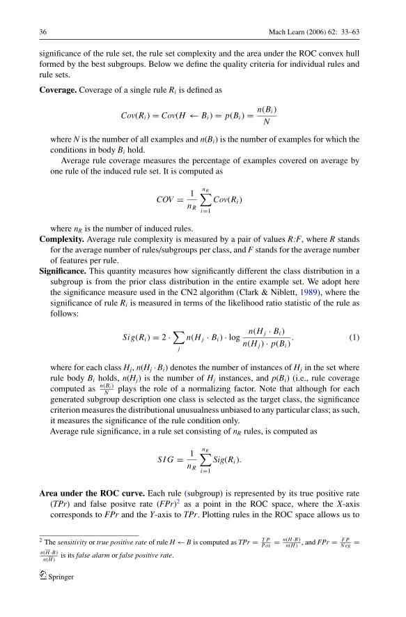
Figure 1 shows examples of ROC diagrams for the Trains domain, plotting the resultsobtained by the weighted covering and standard covering algorithms, respectively. In thisillustrative example we evaluate the induced subgroups on the training set to determine thecoordinates of points in the ROC diagram, and not a separate test set, as is normally the case.

6 Whereas this approach is referred to as additive in Lavrac et al. (2004), another option is the multiplicativeapproach, where for a given parameter γ < 1, weights of positive examples covered by i rules decreaseaccording to γ i. Both approaches have been implemented in CN2-SD and RSD, but additive weights lead tobetter results.

7 Abbreviation ROC denotes Receiver Operating Characteristic.

Springer

Mach Learn (2006) 62: 33–63 41

Fig. 1 ROC diagrams for the Trains domain. The left-hand side diagrams show subgroups discovered whenWest is the target class, and the right-hand side diagrams show subgroups for target class East. The shownsubgroups were constructed by the weighted covering algorithm (upper diagrams) and standard coveringalgorithm (lower diagrams), using the WRAcc and Acc heuristics. Note that subgroups induced using the Accheuristic are very specific and that they all lie on the Y-axis

Weighted relative accuracy of a rule is proportional to the vertical distance of point(TPr,FPr) to the diagonal in the ROC space. To see that this holds, note first that ruleaccuracy p(H | B) is proportional to the angle between the X-axis and the line connecting theorigin (0,0) with the point (TPr,FPr) depicting the rule in terms of its TPr/FPr tradeoff inROC space. So, for instance, all points on the X-axis have rule accuracy equal 0, all pointson the Y-axis have rule accuracy equal 1, and the diagonal represents subgroups with ruleaccuracy p(H), i.e., the prior probability of the positive class. Consequently, all point on thediagonal represent insignificant subgroups.

Using relative accuracy, p(H | B) − p(H), the above values are re-normalized such thatall points on the diagonal have relative accuracy 0, all points on the Y-axis have relativeaccuracy 1 − p(H ) = p(H ) (the prior probability of the negative class), and all points onthe X-axis have relative accuracy −p(H). Notice that all points on the diagonal also haveWRAcc = 0. In terms of subgroup discovery, the diagonal thus represents all (insignificant)subgroups with the same target class distribution as present in the whole population; onlythe generality of these ‘average’ subgroups increases when moving from left to right alongthe diagonal.8

The area under the ROC curve (AUC) can be used as a quality measure for subgroup dis-covery. To compare individual subgroup descriptions, a rule/subgroup description is plotted

8 This interpretation is slightly different in classifier learning, where the diagonal represents random classifiersthat can be constructed without any training.

Springer

42 Mach Learn (2006) 62: 33–63

in the ROC space with its true and false positive rates, and the AUC is calculated. On the otherhand, to compare sets of subgroup descriptions induced by different algorithms, we can formthe convex hull of the set of points with optimal TPr/FPr tradeoff values. The area underthis ROC convex hull indicates the combined quality of the optimal subgroup descriptions,in the sense that it evaluates whether a particular subgroup description has anything to addin the context of all the other subgroup descriptions. This evaluation method has been usedin the experiments in this paper.9

3.7. Constraint-based data mining framework for subgroup discovery

Inductive databases (Imielinsky & Mannila, 1996) provide a database framework for knowl-edge discovery in which the definition of a data mining task (Mannila & Toivonen, 1997)involves the specification of a language of patterns and a set of constraints that a pattern hasto satisfy with respect to a given database. In constraint-based data mining (Bayardo, 2002)the constraints that a pattern has to satisfy consist of language constraints and evaluationconstraints. The first concern the pattern itself, while the second concern the validity of thepattern with respect to a database. The use of constraints enables more efficient induction aswell as focussing the search for patterns on patterns likely to be of interest to the user.

While many different types of patterns have been considered in data mining, constraintshave been mostly considered in mining frequent itemsets and association rules, as well assome related tasks, such as mining frequent episodes, Datalog queries, molecular fragments,etc. Few approaches exist that use constraints for other types of patterns/models, such as sizeand accuracy constraints in decision trees (Garofalakis & Rastogi, 2000), rule induction withconstraints in relational domains including propositionalization (Aronis & Provost, 1994;Aronis et al., 1996), and using rule sets to maximize the ROC performance (Fawcett, 2001).

In RSD, we use a constraint-based framework to handle the curse of dimensionalitypresent in both procedural phases of RSD: first-order feature construction and subgroupdiscovery. We apply language constraints to define the language of possible subgroup de-scriptions, and apply evaluation constraints during rule induction to select the (most) inter-esting rules/subgroups. RSD makes heavy use of both syntactic and semantic constraintsexploited by search space pruning mechanisms. On the one hand, some of the constraints(such as feature undecomposability) are deliberately enforced by the system and pruningbased on these constraints is guaranteed not to cause the omission of any solution. On theother hand, additional constraints (e.g., maximum variable depth) may be tuned by the user.These constraints are designed with the intention to most naturally reflect possible user’sheuristic expectations or minimum requirements on quantitative evaluations of search results.The combination of the above mentioned strategies controlled by constraints is an originalapproach to relational subgroup discovery.

4. RSD propositionalization

In RSD, propositionalization is performed in three steps:

9 This method does not take account of any overlap between subgroups, and subgroups not on the convexhull are simply ignored. An alternative method, employing the combined probabilistic classifications of allsubgroups (Lavrac et al., 2004), is beyond the scope of this paper.

Springer

Mach Learn (2006) 62: 33–63 43

– Identifying all expressions that by definition form a first-order feature (Flach & Lachiche,1999) and at the same time comply to user-defined mode-language constraints. Suchfeatures do not contain any constants and the task can be completed independently of theinput data.

– Employing constants. Certain features are copied several times with some variablesgrounded to constants detected by inspecting the input data. This step includes a sim-plified version of a feature filtering method proposed in Lavrac et al. (1999).

– Generating propositionalized representation of the input data using the generated featureset, i.e., a relational table consisting of truth values of first-order features, computed foreach individual.

4.1. First-order feature construction

RSD accepts feature language declarations similar to those used in Progol (Muggleton,1995). A declaration lists the predicates that can appear in a feature, and to each argumentof a predicate a type and a mode are assigned. In a correct feature, if two arguments havedifferent types, they may not hold the same variable. A mode is either input or output; everyvariable in an input argument of a literal must appear in an output argument of some precedingliteral in the same feature. (Flach & Lachiche, 1999) further dictate the opposite constraint:every output variable of a literal must appear as an input variable of some subsequent literal.Furthermore, the maximum length of a feature (number of contained literals) is declared,along with optional constraints such as the maximum variable depth (Muggleton, 1995),maximum number of occurrences of a given predicate symbol in a feature, etc.

RSD generates an exhaustive set of features satisfying the language declarations as wellas the connectivity requirement, which stipulates that no feature may be decomposable intoa conjunction of two or more features. For example, the following expression does not forman admissible feature

hasCar(A, B), hasCar(A, C), long(B), long(C) (5)

since it can be decomposed into two separate features. We do not construct such decom-posable expressions, as these are redundant for the purpose of subsequent search for ruleswith conjunctive antecedents. Furthermore, as we will show in the experimental part of thepaper, the concept of undecomposability allows for powerful search space pruning. Noticealso that the expression above may be extended into an admissible undecomposable featureif a binary property predicate is added:

hasCar(A, B), hasCar(B, C), long(B), long(C), notSame(B, C) (6)

The construction of features is implemented as depth-first, general-to-specific searchwhere refinement corresponds to adding a literal to the currently examined expression.During the search, each search node found to be a correct feature is listed in the output.

Let us determine the crucial complexity factors in the search for features. Let Mi bethe maximum number of input arguments found in any declared predicate and Mo be theanalogous maximum for output arguments. A currently explored expression f with literals l1,l2, . . . , ln, n < L (where L is the prescribed maximum feature size) can be refined by adding aliteral ln+1, which can be one of D different declared predicates. Each input argument of ln +1

can hold one of the variables occurring as output variables in f or the key variable linking to an

Springer

44 Mach Learn (2006) 62: 33–63

Fig. 2 Left: The number of features as a function of the maximum allowed feature length in the Trainsdomain where all declared predicates have at most one input argument. Right: The same dependence plottedfor the same declaration extended by binary-input property predicate notSame/2

individual (such as A in the examples above). There is at most 1 + n ·Mo such variables andln+1 has at most Mi input arguments. Therefore for each predicate chosen for ln+1, there is atmost (1 + n · Mo)Mi choices of argument variables (output arguments acquire new distinctvariables), that is, the literal ln+1 can be chosen in at most D · (1 + n · Mo)Mi different ways.The search space thus contains at most �L

n=1 D · (1 + n · Mo)Mi ≤ DL · (1 + L · Mo)Mi ·L

search nodes. Two exponential factors are present in this worst-case estimate: Mi — themaximum input arity, and L — the maximum feature length. Out of the two, the formeris of less interest to us, since it is typically set to a small constant in common applicationdomains. For example, in the empirical evaluation (Krogel et al., 2003) conducted on sixbenchmark problems, Mi had the value 1 in four domains and 2 in two domains, in all casesleading to a useful feature set (with respect to the predictive accuracy of the subsequentlyinduced model of data built on the provided features). The latter parameter L is thus a crucialcomplexity factor of the algorithm—therefore it is used as the independent variable in mostof the performance diagrams shown in this paper.

The above worst-case estimate ignores the moding and typing constraints. They mayhowever significantly improve upon the estimate, which we illustrate empirically. The leftpanel of Figure 2 shows the actual number of features as a function of the maximum alloweddefinition length in the Trains domain where Mi = 1 (no predicates with more than oneinput argument are declared). Despite the estimated exponential-in-L growth, the functionactually becomes constant at L = 16. This is no longer the case when binary-input predicatenotSame/2 is further declared (allowing to construct features such as (6) above). Here Mi

= 2 and the number of features grows exponentially with L.RSD implements several pruning techniques to reduce the number of examined expres-

sions, while preserving the exhaustiveness of the resulting feature set.First, suppose that the currently explored expression f of length n contains o output

variables not appearing also as input variables in f. Let the maximum number of inputarguments of a predicate among all available background predicates be Mi and L be themaximum length of a feature. Then

Rule 1. Once L − n ≤ oMi

, prune all descendants of f reached by adding a structuralliteral to it.

In other words, if the inequality holds, the algorithm will no longer consider to addstructural predicates when refining f. By doing so it would introduce one or more new outputvariables; a simple calculation yields that there would not be enough literal positions left tomake all output variables appear also as inputs.

Springer

Mach Learn (2006) 62: 33–63 45

The following two pruning rules exploit the constraint of feature undecomposability. Theconstraint is verified by maintaining a set ϑeq(f) of equivalence classes of non-key variablesin each explored expression f. Two non-key variables X, Y fall in the same equivalence classiff they are connected, i.e., if they both appear as arguments in one literal of the expression,or there is a non-key variable Z such that X, Z are connected and Z, Y are connected.Expression f is a feature only if |ϑeq( f )| = 1. Note that a feature may be reached by refininga decomposable node. The following two pruning rules cut off the search subspaces whichsurely contain only decomposable nodes. Let us call a literal primary if all its input argumentshold the key variable.

Rule 2. If expression f is a non-empty conjunction, prune all its descendants reached byadding a primary property literal to it.

Rule 2 expresses the simple insight that adding a primary property literal to a featuredefinition will yield a decomposable feature.

Rule 3. Let expression f contain a primary literal lp.

1. If lp is a property literal, prune all descendants of f.2. If lp is a structural literal and Mi = 1, prune all descendants reached by adding a

primary structural literal to f.

The first item of pruning Rule 3 again avoids combining a primary property literal with anyother literals. Now consider the case when the maximum input arity of available predicatesis equal to 1 (the second item of Rule 3). This is natural in frequent cases when eachstructural predicate serves for addressing a part or a substructure of a single structure andproperty predicates do not relate two or more objects. For example, the earlier addressedTrains domain is a typical representant of the situation if the declared language excludes thebinary predicate notSame/2 relating two cars. The second item of Rule 3 then capturesthe following idea. To reach a contradiction, let us assume that we can in fact arrive to anadmissible feature definition that contains two primary structural literals l1 and l2. Let oi besome output variable of li (i = 1, 2). Since the maximum input arity is 1, o1 and o2 cannotbe connected and the feature would be decomposable, that is, inadmissible.

Finally, it can be shown that Rules 2 and 3 cut off all decomposable nodes in the searchtree when amax = 1 and therefore we can skip decomposability checks as Rule 4 dictates.

Rule 4. If Mi = 1, skip all decomposability checks.

Figure 3 illustrates the impact of the described pruning techniques on the efficiency ofthe feature construction algorithm.

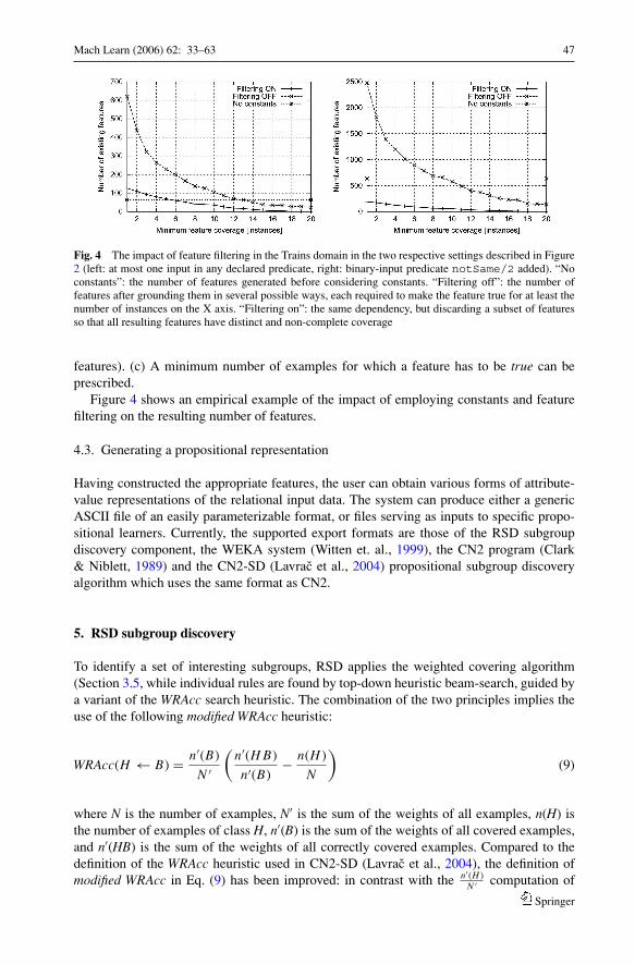
4.2. Employing constants and feature filtering

After constructing a constant-free feature set, RSD proceeds to ground selected variablesin the features with constants extracted from the input data in the following manner. Theuser may declare a special property predicate instantiate/1, just like other propertypredicates. An occurrence of this predicate in a feature with some variable V as its argumentspecifies that all occurrences of V in the feature should be eventually substituted with aconstant. The instantiate/1 literal may appear several times with different variables

Springer

46 Mach Learn (2006) 62: 33–63

Fig. 3 Empirical example of the impact of search space pruning during syntactic feature construction in theTrains domain. The diagrams on the left show the number of admissible features in the two settings describedin Figure 2 (top: at most one input in any declared predicate, bottom: additional binary-input predicate) withthe growing maximum feature length: we redisplay these dependencies for ease of comparison. To the rightof each of them, we plot the time taken by the algorithm to complete the feature construction in the respectivesetting with pruning off and on. In the case of only-unary-properties (top), the number of features eventuallystops growing, and so does the construction time taken by the pruning-enhanced algorithm as it correctlyeliminates the growing search subspaces containing no correct feature. On the contrary, the non-pruningalgorithm maintains its exponential time complexity. In the case of additional binary property notSame/2(bottom), the time dependencies exhibit a similar shape, however, the efficiency gain of the pruning versionis still essential

in a single feature. A number of different features are then generated, each corresponding toa possible grounding of the combination of the indicated variables. We consider only thosegroundings which make the feature true for at least a pre-specified number of individuals.

For example, after consulting the input data, the constant-free expression

hasCar(A, B), hasLoad(B, C), hasShape(C, D), instantiate(D) (7)

is replaced by a set of features, in each of which the instantiate/1 literal is removedand the D variable is substituted by a constant making the conjunction true for at least oneindividual, for example

hasCar(A, B), hasLoad(B, C), hasShape(C, rectangle) (8)

Feature filtering takes place within the described step of employing constants and con-forms to the following constraints. (a) No feature should have the same Boolean value for allthe examples. (b) No two features should have the same Boolean values for all the examples(in this case, a single feature is chosen to represent the class of semantically equivalent

Springer

Mach Learn (2006) 62: 33–63 47

Fig. 4 The impact of feature filtering in the Trains domain in the two respective settings described in Figure2 (left: at most one input in any declared predicate, right: binary-input predicate notSame/2 added). “Noconstants”: the number of features generated before considering constants. “Filtering off”: the number offeatures after grounding them in several possible ways, each required to make the feature true for at least thenumber of instances on the X axis. “Filtering on”: the same dependency, but discarding a subset of featuresso that all resulting features have distinct and non-complete coverage

features). (c) A minimum number of examples for which a feature has to be true can beprescribed.

Figure 4 shows an empirical example of the impact of employing constants and featurefiltering on the resulting number of features.

4.3. Generating a propositional representation

Having constructed the appropriate features, the user can obtain various forms of attribute-value representations of the relational input data. The system can produce either a genericASCII file of an easily parameterizable format, or files serving as inputs to specific propo-sitional learners. Currently, the supported export formats are those of the RSD subgroupdiscovery component, the WEKA system (Witten et. al., 1999), the CN2 program (Clark& Niblett, 1989) and the CN2-SD (Lavrac et al., 2004) propositional subgroup discoveryalgorithm which uses the same format as CN2.

5. RSD subgroup discovery

To identify a set of interesting subgroups, RSD applies the weighted covering algorithm(Section 3.5, while individual rules are found by top-down heuristic beam-search, guided bya variant of the WRAcc search heuristic. The combination of the two principles implies theuse of the following modified WRAcc heuristic:

WRAcc(H ← B) = n′(B)

N ′

(n′(H B)

n′(B)− n(H )

N

)(9)

where N is the number of examples, N′ is the sum of the weights of all examples, n(H) isthe number of examples of class H, n′(B) is the sum of the weights of all covered examples,and n′(HB) is the sum of the weights of all correctly covered examples. Compared to thedefinition of the WRAcc heuristic used in CN2-SD (Lavrac et al., 2004), the definition ofmodified WRAcc in Eq. (9) has been improved: in contrast with the n′(H )

N ′ computation of

Springer

48 Mach Learn (2006) 62: 33–63

the prior probability in CN2-SD which changes with changed example weights, in RSD theprior probability computation n(H )

N remains unchanged.To add a rule to the generated rule set, the rule with the maximum modified WRAcc value

is chosen from the set of searched rules not yet present in the rule set generated so far.The constraints employed in the subgroup search include the language constraint of

the maximal number of features considered in the subgroup description as well as severalevaluation constraints. These include the minimal value of the significance formula (Clark& Niblett, 1989) for each subgroup, as well as a minimal value threshold for the modifiedWRAcc function, which is exploited for sake of pruning.

Two pruning rules are used in the beam-search. According to the first, all refinements ofa node will be pruned, if that node stands for a rule covering only instances of the targetclass, as such a rule cannot be improved by a refinement. Furthermore, if minimal value t isprescribed for WRAcc, we prune all refinements of rule H ← B if the inequality

n′(B)

N ′

(1 − n(H )

N

)< t (10)

holds, as clearly no refinement thereof can yield a WRAcc value higher than the left-handside of the inequality (weighted coverage will not grow when specializing, while weightedaccuracy cannot exceed 1). Constraint (10) thus ensures that no rule is induced whosecoverage n′(B)

N ′ is so small that even if the rule had perfect accuracy p(H | B) = 1, its coveragevs. relative accuracy tradeoff computed by WRAcc would have been below t.

6. Experimental domains

In addition to three popular ILP data sets, the East-West trains (Trains), the King-Rook-King illegal chess endgame positions (KRK) and mutagenicity prediction (Mutagenesis), wehave performed the experimental evaluation of RSD also on two other domains: a real-lifetelecommunications problem (Telecom) and the analysis of traffic accidents (Traffic). TheTrains problem was used in earlier sections for explanatory purposes only.

6.1. Three ILP domains

We performed experiments on three popular ILP data sets: Trains, KRK and Mutagenesis.

Trains. We chose the 20 trains East-West challenge (Michie et al., 1994) as an illustratingexample earlier in this paper. For these trains, information is given about their cars andthe loads of these cars. The original classification task was to discover (low-complexity)models that classify trains as heading East or West. The subgroup discovery task addressedin this paper is to discover subgroups that are sufficiently large and biased towards oneof the two classes: East and West.

KRK. In the chess endgame domain White King and Rook versus Black King, takenfrom (Quinlan, 1990) (first described in Muggleton et al. (1989)), the target relationillegal(A, B, C, D, E, F) states whether a position where the White Kingis at file and rank (A, B), the White Rook at (C, D) and the Black King at (E, F)is an illegal White-to-move position. For example, illegal (g,6,c,7,c,8) is apositive example, i.e., an illegal position. Two background predicates are available: lt/2expressing the less than relation on a pair of ranks/files, andadj/2 denoting the adjacency

Springer

Mach Learn (2006) 62: 33–63 49

relation on such pairs. The data set consists of 1000 instances. The original predictiveKRK task aimed at best distinguishing between illegal and legal chess endgame positions,whereas the subgroup discovery task aims at detecting groups of chessboard positions,distinguishable by means of the background relations, which contain an unusually largeproportion of illegal/legal positions. In the KRK domain we do not expand features byinstantiating variables to constants (as described in Section 4.2). This problem is thus‘purely relational’.

Mutagenesis. The Mutagenesis problem defined in Srinivasan et al. (1996) is a variant of theoriginal data named NS+S2 (also known as B4) that contains information about drugs:their chemical properties, the drugs’ atoms and the bonds between the atoms. The originalMutagenesis learning task was to predict whether a drug is mutagenic or not. The sepa-ration of data into ‘regression-friendly’ (188 instances) and ‘regression-unfriendly’ (42instances) subsets as described by Srinivasan et al. (1996) is followed in our experiments.Our experiments concentrate on subgroup discovery from the ‘regression-friendly’ subsetconsisting of 188 instances.

6.2. The Telecom domain

We have applied RSD to a real-life problem in telecommunications. An extensive descriptionof the nature of the data as well as tasks and problems that appear in this domain can befound in Zelezny et al. (2000, 2002).

The data represent incoming calls (1995 items thereof) to an enterprise. Each call isanswered by a human operator and in the usual case further transferred to an attendantdistinguished by his/her line number. Further call transfers may also occur. Each sequence ofsuch transfers is tracked by a computerized exchange and related data are stored in a log file.By a suitable transformation thereof, one can form a relation incoming/5, represented byground facts of the formincoming (date, time, caller, operator, result). The argument resulteither takes a constant value or is a recursively defined function, so that result ∈ {talk,unavailable, transfer ([ln1, ln2, . . . , lnn], result)}, where ln1 ... lnn denote linenumbers to which transfer attempts were made (in the first n − 1 cases unsuccessfully andin the n-th case with outcome result). For example, the following fact

incoming(date(10,18),time(13,37,29),[0,6,4,8,2,5,6,8,4,9],32,transfer([16,12],transfer([26],talk)))

describes a call from phone number 0648256849 at 13:37:29 on 10/18 received by theoperator on line 32. The operator first tried to transfer the caller to line 16 without success,and then transferred him/her successfully to line 12. The person on line 12 further redirectedthe caller to line 26. After a talk with line 26, the call was terminated.

We divided all instances of incoming transferred calls into 25 classes determined by theline to which the operator tried to transfer the caller first. The arguments of the traininginstances thus consist of the first four arguments of incoming/5, and the class label ln1.The goal of subgroup discovery is to find subgroups biased to specific classes (destinationsof first call transfer) which may be used to support operators’ decision making.

Let us now comment on two of the available background relations. The predicate pre-fix(Number,Prefix) is true whenever the second (output) argument is the prefix (ofany length) of the first (input) argument. For instance, regarding the example given above,prefix([0,6,4,8,2,5,6,8,4,9],[0,6,4]) is true. This background predicateproved useful in previously published results, since it is able to bind callers from the samearea, city, company, office etc.

Springer

50 Mach Learn (2006) 62: 33–63

Table 2 The meaning and the distribution of class values in the UK Trafficchallenge data set

Code Meaning of class values Distribution %Class0 No skidding, jack-knifing or overturning 64.26

Class1 Skidded 22.07Class2 Skidded and overturned 7.27Class3 Jack-knifed 0.20Class4 Jack-knifed and overturned 0.19Class5 Overturned 6.01

Another background predicate (prev\ attempt/6) reflects the fact that a line desiredby the caller may often be determined by looking at the caller’s recent attempts to reach aperson, i.e., by inspecting past records (w.r.t. the time-label of the current example) in theincoming/5 relation. For example, the goalprev attempt(date(10,18),time(13,37,29),[0,6,4,8,2,5,6,8,4,9],Line, When, Result)

will succeed with the result

Line = 10, When = today, Result = unavailable

provided the caller 0648256849 failed to reach line 10 on 10/18 before 13:37:29. Note thatthe prev attempt/6 may yield multiple outputs for a given instantiation of the inputarguments.

6.3. The UK Traffic Accidents Domain

The UK Traffic data set includes the records of all the accidents that happened on theroads of Great Britain between years 1979 and 1999 (Flach et al., 2003). It is a relationaldata set consisting of 3 related data tables: the ACCIDENT data, the VEHICLE data and theCASUALTY data. The ACCIDENT data consists of the records of all accidents that happenedin the given time period; VEHICLE data includes data about all the vehicles involved inthese accidents; CASUALTY data includes the data about all the casualties involved in theaccidents. Consider the following example: ‘Two vehicles crashed in a traffic accident andthree people were seriously injured in the crash’. In terms of the TRAFFIC data set this isrecorded as one record in the ACCIDENT data table, two records in the VEHICLE data tableand three records in the CASUALTY data table. Every data table is described by around 20attributes and consists of more than 5 million records.

The UK Traffic challenge data set is formed of a subset of records of the above dataset. The task of the challenge was to generate classification models to predict skidding andoverturning. As the class attribute Skidding and Overturning appears in the VEHICLE datatable, data tables ACCIDENT and VEHICLE were merged in order to make this a non-relational learning problem. Furthermore, a randomly sampled subset of 5940 records fromthis merged data table was selected for learning and another sample of 1585 records wasselected for testing. The class attribute Skidding and Overturning has six possible values.The meaning of these values and the distribution of class values in the training and test setsare shown in Table 2.

Springer

Mach Learn (2006) 62: 33–63 51

Table 3 Examples of generated features

KRK f6(A):-king1 rank(A,B),rook rank(A,C),adj(C,B).Meaning First king’s rank adjacent to rook’s rank.

Mutagenesis f12(A):-atm(A,B),atm chr(B,C),lteq c(C,0.142).Meaning A compound contains an atom with charge less or equal to 0.142.

Mutagenesis f31(A):-benzene(A,B),benzene(A,C),connected(C,B).Meaning Presence of two connected benzene rings in the compound.

Telecom f99(A):-ext number(A,B),prefix(B,[0,4,0,7]).Meaning Caller’s number starts with 0407.

Telecom f115(A):-call date(A,B),call time(A,C),ext number(A,D),prev attempt(B,C,D,[3,1],today,unavailable).

Meaning The caller of the current call has today tried to reach line 31, which was unavailable.

While the original task of the challenge was to generate classification models to predictskidding and overturning, in our case, the task is to find subgroup descriptions representinginteresting skidding and overturning patterns appearing in the Traffic challenge data set.

7. RSD propositionalization: Experimental evaluation

This section presents the experimental results. Experiments with feature construction andfiltering are illustrated in three domains: KRK, Telecom and Mutagenesis. An experimentalcomparison of the RSD propositionalization procedure with the original first-order featureconstruction procedure (Flach & Lachiche, 1999; Lavrac & Flach 2001; Kramer et al.,2001) as implemented in SINUS (Krogel et al., 2003) is performed in KRK, Trains andMutagenesis.

7.1. Evaluation of feature construction and filtering

To generate features for KRK and Telecom, we use the background predicates described inthe domains descriptions. For the KRK domain, we also allow to generate features in theform of a negation of a complete literal conjunction.

Figure 5 reflects the quantitative characteristics of RSD syntactic feature construction andthe effect of pruning in the three domains, from the viewpoint we took in the Trains domainin Figure 3. The efficiency gain by the earlier described search space pruning techniques isnot very significant in the KRK domain, but becomes essential with growing feature lengthin Telecom and Mutagenesis.

Table 3 shows examples of features generated in the KRK, Mutagenesis and Telecomdomains.

7.2. Experimental comparison with SINUS

This section compares the RSD propositionalization procedure with the first-order featureconstruction procedure (Flach & Lachiche, 1999; Lavrac & Flach, 2001; Kramer et al.,2001) implemented in SINUS (Krogel et al., 2003).

SINUS was first implemented as an extension to the original LINUS transformational ILPlearner (Lavrac & Dzeroski, 1994). LINUS performs the transformation to a propositionalrepresentation by considering only possible applications of background predicates on the

Springer

52 Mach Learn (2006) 62: 33–63

Fig. 5 Number of features (left) and impact of pruning in RSD syntactic feature construction on efficiency(right) in KRK, Telecom and Mutagenesis, shown in dependence to the maximum allowed length of a feature.This viewpoint corresponds to Figure 3 for the example domain of Trains

arguments of the target relation, taking into account the types of arguments. The clauses itlearns are constrained. The development of DINUS (Lavrac & Dzeroski, 1994) relaxed thisbias so that non-constrained clauses can be constructed provided that the clauses involvedare determinate. SINUS was later extended to perform propositionalization by extendedfirst-order feature construction described in Flach and Lachiche (1999), Lavrac and Flach(2001) and Kramer et al., (2001).10

The RSD propositionalization has the following advantages compared to SINUS. It pro-vides a declaration language similar to Progol for fine-tuning syntactic constraints on features,it verifies the undecomposability of features and offers improvements (pruning techniques inthe feature search, coverage-based feature filtering). These improvements lead to improvedefficiency of propositionalization as shown in the experiments of this section.

10 Detailed information about SINUS is available from the SINUS website athttp://www.cs.bris.ac.uk/home/rawles/sinus/ .

Springer

Mach Learn (2006) 62: 33–63 53

Table 4 Indicators of running times (different platforms, cf. text) andsystems providing the feature set for the best-accuracy result in eachdomain

Problem Running times J48 Accuracy

RSD SINUS RSD SINUS

Trains <1 sec 2 to 10 min 65.0% 70.0%KRK <1 sec 2 to 6 min 96.3% 95.0%Mutagenesis 5 min 6 to 15 min 92.55% 84.6%

As RSD and SINUS are implemented in different languages (interpreters) and operateon different hardware platforms, exact comparison of runtime efficiency is not possible. Asin Krogel et al. (2003), for each domain and system we report the approximate runningtimes, averaged over multiple feature construction runs, varying in the language constraintsand producing feature sets of different sizes. RSD ran under the Yap Prolog on a Celeron800 MHz computer with 256 MB of RAM. SINUS ran under SICStus Prolog11 on a SunUltra 10 computer. Table 4 shows running times of the propositionalization systems on thelearning tasks (with best results indicated in bold). The table also provides 10-fold stratifiedcross-validation accuracy results of applying the J48 propositional learner (a reimplemen-tation of C4.5 (Quinlan, 1993) available in WEKA (Witten & Frank, 1999)), supplied withpropositionalized data based on feature sets of varying size obtained from the two proposi-tionalization systems. To test the performance of the two systems, producing the accuracyresults in Table 4, RSD and SINUS were used to construct features by different parametersettings; the results of 10-fold stratified cross-validation for the best setting are shown.

Different performance of RSD and SINUS are due to their different ways of constrain-ing the language bias. RSD wins in the KRK domain and Mutagenesis. While the gap onKRK seems little significant, the result obtained on Mutagenesis with RSD’s 25 features12 iscompetitive to the best results reported in the ILP literature. Whether the apparent efficiencysuperiority of RSD w.r.t SINUS is due to the RSD’s pruning mechanisms, or the implemen-tation in the faster Yap Prolog, or a combined effect thereof has to be investigated in moredepth in future work.

8. RSD subgroup discovery: Experimental evaluation

For the experimental domains Trains, KRK, Mutagenicity and Telecom, parts of the experi-mental settings overlap, and parts are unique for each of the domains. The common parts ofthe experimental procedures are outlined below. A separate evaluation procedure is used inthe Traffic challenge domain as the goal is to compare RSD with SubgroupMiner in termsof the AUC performance.

The RSD algorithm was run as follows.

11 It should be noted that SICStus Prolog is generally considered to be several times slower than Yap prolog.

12 The longest have 5 literals in their bodies. Prior to irrelevant-feature filtering conducted by RSD, the featureset had 533 features.

Springer

54 Mach Learn (2006) 62: 33–63

– For each dataset we first ran the RSD propositionalization procedure. We generated a setof features and—when applicable—expanded the set with features containing variableinstantiations. We then used the feature sets to produce a propositional representation ofeach of the data sets. The results of this evaluation were presented in Section 7.1.

– We then ran the RSD subgroup discovery procedure to construct interesting subgroupsfrom the propositional data. In this procedure we have subsequently exchanged the RSD’sWRAcc heuristic with the standard accuracy (Acc) heuristic, and the RSD’s weighted cov-ering algorithm with the standard covering algorithm, thereby testing four configurationsof the method. Results of each are compared in terms of subgroup interestingness criteria.See the list of subgroup evaluation criteria in Section 2 and the results of the evaluation inSection 8.1.

The generation of stratified cross-validation splits and subsequent assessment of resultingrules is done automatically by the RSD system. The experiments are repeatable, as the RSDpackage available at http : //labe.felk.cvut.cz/ ∼ zelezny/rsd contains scripts neededto conduct the experimental procedures automatically to achieve the results presented below.

8.1. Subgroup discovery evaluation results

In the experiments we used different variants of the RSD rule learning algorithm by alteringthe covering strategy and the heuristic function used to construct sets of subgroup-describingrules.

Achieved results and characteristics of discovered rules are shown in Table 5, whereAlgo refers to the combination of the search heuristic (A – accuracy, W – weighted relativeaccuracy) and the covering algorithm (C – covering, W – weighted covering using additiveweights). Results are evaluated in terms of the following interestingness criteria: SIG –significance, COV - coverage, AUC – area under the ROC curve, R : F – average numberof rules per class : average number of features per rule, R′ : F′ – the same as above, butconsidering only the rules on the ROC convex hull. The reported results are averages obtainedin 10-fold stratified cross-validation, along with the corresponding standard deviations.

Rule generation for a given class was terminated if the search space was completely ex-plored or the maximal number of subgroup rules was generated (10 subgroup rules generatedfor KRK and Telecom, and 5 for Mutagenesis).

The most important observation about the results in Table 5 is that, in terms of allthe quality criteria, the RSD’s WRAcc heuristic very significantly improves the performancecompared to the standard accuracy heuristic. Overall, the combination of the WRAcc heuristicwith the strategy of example weighting used in the weighted covering algorithm yields the bestresults. This agrees with the findings in (Lavrac et al., 2004), where a more extensive empiricalevaluation was conducted on a collection of (non-relational) subgroup discovery problems,comparing the CN2 algorithm with CN2 incorporating a variant of the WRAcc heuristic, andfurther with the CN2-SD system (which incorporates a variant of the WRAcc heuristic andthe weighted covering algorithm). These three algorithms roughly correspond to the methodswe denote above (in Table 5) as AC, WC, and WW, respectively. The combination of theaccuracy heuristic with example weighting AW performs worse in the domains considered.

8.2. Expert analysis of induced subgroups

We now present selected subgroups, discovered by RSD in the KRK and Telecom domains,to illustrate the character of induced rules. We also present their pie-chart visualization.

Springer

Mach Learn (2006) 62: 33–63 55

Table 5 Results of ten-fold cross-validation obtained by the RSD algorithm in the KRK, Mutagenesis andTelecom domains (with standard deviations in parentheses)

Performance ComplexityAlgo SIG COV AUC R : F R′ : F′

KRKAC 2.29 1.82% 0.54 10.00 : 2.19 10.00 : 2.19

(0.59) (0.37) (0.01) (0.00 : 0.04) (0.00 : 0.04)AW 2.59 1.80% 0.54 10.00 : 2.57 10.00 : 2.57

(0.84) (0.48) (0.01) (0.00 : 0.05) (0.00 : 0.05)WC 9.12 7.92% 0.72 7.50 : 2.80 6.50 : 2.78

(1.28) (0.44) (0.02) (0.00 : 0.06) (0.44 : 0.06)WW 11.14 10.64% 0.72 10.00 : 2.77 6.00 : 2.64

(2.05) (0.64) (0.02) (0.00 : 0.04) (0.52 : 0.06)MutagenesisAC 1.99 11.33% 0.69 10.00 : 2.16 10.00 : 2.16

(0.92) (3.74) (0.07) (0.00 : 0.07) (0.00 : 0.07)AW 1.33 7.62% 0.58 10.00 : 2.50 10.00 : 2.50

(1.05) (4.88) (0.06) (0.00 : 0.11) (0.00 : 0.11)WC 4.22 35.81% 0.86 3.70 : 1.73 2.30 : 1.62

(1.22) (6.44) (0.06) (0.82 : 0.33) (0.48 : 0.22)WW 7.48 40.58% 0.90 10.00 : 2.63 6.50 : 2.43

(1.28) (4.74) (0.04) (0.00 : 0.07) (0.97 : 0.11)TelecomAC 2.90 0.37% 0.55 7.36 : 2.39 6.88 : 2.47

(0.38) (0.05) (0.02) (0.12 : 0.04) (0.19 : 0.04)AW 2.56 0.26% 0.55 9.96 : 2.56 9.60 : 2.61

(0.52) (0.04) (0.02) (0.07 : 0.03) (0.07 : 0.03)WC 11.29 4.98% 0.67 6.12 : 2.17 5.20 : 2.28

(1.71) (0.54) (0.02) (0.16 : 0.04) (0.16 : 0.04)WW 12.00 4.07% 0.70 9.64 : 2.06 6.68 : 2.29

(1.05) (0.41) (0.01) (0.12 : 0.01) (0.20 : 0.03)

Table 6 A subgroup description induced in the KRK domain in the form H ← B [TP,FP], its interpretationand definitions of features appearing as literals in the conjunctive antecedent of a rule describing the subgroup

Subgroup KRK1 for target class: legallegal(A) ← f139(A) ∧ f145(A) ∧ f133(A) [279,4]f139(A):-not(rook rank(A,B),king2 rank(A,C),adj(C,C),adj(C,B)).f145(A):-not(rook file(A,B),king2 file(A,C),adj(C,C),adj(C,B)).f133(A):-not(king1 file(A,B),king2 file(A,C),adj(C,C),adj(C,B)).Configurations where rook’s rank is not adjacent to second king’s rank and rook’s file not adjacent to

second king’s file and first king’s file not adjacent to second king’s file (note that adj(C,C) is alwaystrue, i.e. redundant).

Table 6 presents a subgroup, induced in the KRK domain, and lists the Prolog notation ofthe features used as antecedent literals in the rule that describes the subgroup. The graphicalpresentation of the class distribution and coverage of the subgroup, illustrated at the right-hand side of Figure 6, is complemented in Table 6 by a verbal description of the subgroup,together with the number of true positive (TP) and false positive (FP) examples covered.

Springer

56 Mach Learn (2006) 62: 33–63

Fig. 6 Left: Subgroup Trains1 described in Table 1 of Section 2. Right: Subgroup KRK1 described inTable 6 of this section

Fig. 7 Left: Prior distribution of classes in the Telecom domain. Right: Subgroup Tele1 described in Table7 of this section

Fig. 8 Left: Subgroup Tele2, Right: Subgroup Tele4, both described in Table7 of this section

Figures 6–8 show pie-chart representations of the distributional characteristics of inducedsubgroups. In the outer pie, each area representing a class is proportional to the frequency ofthat class in the data set. Similarly, areas in the inner pie are proportional to the frequenciesof corresponding classes in the subgroup. The ratio of the overall area of the inner pie to thearea of the whole pie is the ratio between the number of instances included in the subgroupin and the number of all the instances in the respective data set.

In the Telecom domain, although exactly one class is the target, it often follows from theillustrated posterior distribution that the rule consequent can naturally be interpreted as a

Springer

Mach Learn (2006) 62: 33–63 57

Table 7 Telecom subgroup descriptions in the form H ← B [TP,FP], definitions of used features, andsubgroup interpretation including expert’s comments

Tele1: line21(A) ← f40(A) [56,268]f40(A):-call date(A,B), dow(B,fri).Calls received on Fridays.Expert’s evaluation: Not a novel information.

Tele2: line11(A)← f132(A) [32,0]f132(A):-ext number(A,B), prefix(B,[8,5,1,3,1,1,1,1]).Calls received from number 85131111.Expert’s explanation: The caller is the secretary’s husband. She does not have a direct-access line, thus this

call is transferred by an operator.Expert’s evaluation: Novel information.Remark. Although the last literal formally identifies a prefix of the calling number, it is in fact the complete

number of the caller.

Tele3: line21(A) ← f54(A) [81,254]f54(A):-ext number(A,B), prefix(B,[0,4]).Calls received from a number that starts with 04.Expert’s explanation: Prefix 04 is too general (code covers a large area) to find an explanation.Expert’s evaluation: Novel information. Uncertain.

Tele4: line28(A) ← f7(A) [22,11]f7(A):-call date(A,B), call time(A,C),ext number(A,D), prev attempt(B,C,D,[2,1],last hour,unavailable).

Calls received from a caller who has in the last hour attempted to directly (not through an operator) reachline 28, which was unavailable.

Expert’s explanation: It is plausible that people try line 28 as the second attempt when line 21 isunavailable. Subgroup probably mostly covers people with technical difficulties with a product sold byperson on line 21.

Expert’s evaluation: Novel information.

disjunction of classes. This applies in cases when a subgroup contains instances of only afew classes, as opposed to the prior distribution of 25 classes.13

We now present the descriptions of some of the discovered subgroups in Telecom, withcomments from the domain expert on the descriptions in Table 7 and the distributionalcharacteristics of the subgroups in terms of the number of true positives (TP) and falsepositives (FP).

Expert analysis of the induced rules shows that some of them identify novel and interestinginformation. Especially revealing are the comments related to the changes of class frequencyassociated with the rules, as illustrated in the pie-charts. In the overall distribution, callsto line 21 are the most common. The expert commented that this reflects his expectations,as the person at line 21 is a marketer, and people interested in products call this linemost frequently. In subgroup Tele1, there is (a) an increase in line 21 frequency: clientsnot receiving an ordered package often wait until Friday and then complain with line 21;and (b) a decrease in line 13 frequency: the person at line 13 mostly collaborates withdealers who have less business on Fridays. For subgroup Tele4 there is (a) an increasein line 28 frequency: repeated attempts to reach line 28, and (b) an increase in line 21

13 Note that only 15 classes are visible in the outer pies in the Telecom domain, as instances of the remaining10 classes are rare and thus below the graphics resolution.

Springer

58 Mach Learn (2006) 62: 33–63

Table 8 Performance comparison of Aleph and the AC and WW variants of theRSD algorithm in terms of average significance (SIG), coverage (COV) and areaunder the ROC curve (AUC)

Domain Algo SIG COV AUC

KRK Aleph 2.30 1.18% 0.56AC 2.29 1.82% 0.54WW 11.14 10.64% 0.72

Muta Aleph 1.40 10.39% 0.72AC 1.99 11.33% 0.69WW 7.48 40.58% 0.90

Telecom Aleph 5.24 0.27% 0.75AC 2.90 0.37% 0.55WW 12.00 4.07% 0.70

frequency: the person at line 28 works as technical support for products sold by person online 21.

8.3. Experimental comparison with Aleph

Having compared the four discovery strategy variants within the single RSD system inSection 8.1, we now compare RSD with the relational classification rule learner Aleph,using again the KRK, Telecom and Mutagenesis datasets. Aleph is a system for relational ruleinduction implementing the basic principles described in Muggleton (1995). Unlike RSD,Aleph directly conducts search in a set of first-order rules without prior propositionalizationof the learning data. As a classificatory induction system, Aleph uses the standard (non-weighted) example covering strategy for constructing a rule set, and function f(R) = n+(R) −n−(R) is used as the search heuristic, where n+(R) and n−(R) are the numbers of positive andnegative examples covered by rule R, respectively.

Table 8 compares the qualities of subgroups corresponding to rules discovered by Alephwith those produced by the AC and WW variants of RSD (the last two are repeated fromTable 5). The results were obtained by the same measurement procedure as in Section8.1. As Aleph is a binary-class learner, the 25 class Telecom problem was split into 25tasks, each time with one class representing the positive examples and all other classesrepresenting the negative examples. The final results are averaged over all the 25 learningtasks.

The basic trend observed in the results is that subgroups corresponding to rules foundby Aleph exhibit qualities much closer to those discovered by the AC, rather than the WWvariant of RSD. The main difference between Aleph and the AC variant of RSD is the initialpropositionalization of data performed by the latter algorithm. The results thus suggestthat propositionalizing the learning data does not incur, at least in the tested domains, adetrimental effect on the resulting subgroup qualities.

8.4. Experimental comparison with SubgroupMiner

We further compared RSD to the relational subgroup discovery system SubgroupMiner(Kloesgen & May, 2002). While RSD accepts intensional definitions of background relations,SupgroupMiner requires the input to be in the form of relational tables (ground facts).

Springer

Mach Learn (2006) 62: 33–63 59

This requirement on data form is met in the Traffic challenge problem, which alreadyserved for a mutual comparison of subgroup discovery algorithms in Kavsek and Lavrac(2004).

The task addressed is to find subgroup descriptions representing interesting skid-ding and overturning patterns appearing in the Traffic challenge data set consist-ing of 5940 randomly sampled records from the original ACCIDENT and VEHI-CLE tables. Recall that the class attribute Skidding and Overturning has six possi-ble values: Class0: No skidding, jack-knifing or overturning; Class1: Skidded; Class2:Skidded and overturned; Class3: Jack-knifed; Class4: Jack-knifed and overturned; andClass5: Overturned.

We here adhere to the experimental setting of Kavsek and Lavrac (2004), followingthe same results presentation and comparison of the ROC convex hulls obtained frombest subgroup descriptions induced by each of the two compared subgroup discoverysystems.

The TPr and FPr characteristics of subgroup descriptions induced by the two respec-tive systems for three selected values of the target attribute (Class0: No skidding, jack-knifing or overturning; Class1: Skidded; and Class5: Overturned) are plotted in Figure 9.In these experiments, RSD was run in the WW setting of Table 5, using the weighted cov-ering algorithm and the modified weighted relative accuracy heuristic. The two systemsidentify best subgroups on the ROC convex hull of roughly similar quality. However, Sub-groupMiner induces a much larger set of subgroups, some lying much below the ROCcurve.

9. Conclusions and further work

This paper presents an approach to relational subgroup discovery, whose origins are basedon the recent developments in subgroup discovery (Wrobel, 2001; Lavrac et al., 2004)and propositionalization through first-order feature construction (Flach & Lachiche, 1999;Lavrac & Flach, 2001; Kramer et al., 2001). It presents constraint-based relational subgroupdiscovery algorithm RSD which transforms a relational subgroup discovery problem to apropositional one, through efficient first-order feature construction. Efficiency is boostedmainly through exploiting language and evaluation constraints for pruning.

Concerning propositionalization, our empirical results demonstrate that the strategy im-plemented in RSD represents an advance over the original first-order feature constructionprocedure (Flach & Lachiche, 1999; Lavrac & Flach, 2001) in terms of runtime efficiency.Although the efficiency gain is rather negligible in the KRK domain, it is significant in boththe Telecom and Mutagenesis domains. Furthermore, additional experiments with classifi-catory induction using the generated propositional form indicate that RSD produces featuresleading to high classification accuracy. Lastly, absolute-runtime comparisons with SINUSwhich implements the propositionalization procedure described in Flach and Lachiche (1999)and Lavrac and Flach (2001) indicate the superiority of RSD, although these figures arenot conclusive due to the inherently different software and hardware used by RSD andSINUS.

Following the data propositionalization step, four variants of the core subgroup discoveryRSD algorithm were tested, by combining the standard accuracy and the weighted accuracysearch heuristic used in the construction of individual rules, with the standard covering andweighted covering algorithm used in the construction of a set of rules. The WRAcc heuristiccombined with the weighted covering algorithm is the preferred combination (due to an

Springer

60 Mach Learn (2006) 62: 33–63

Fig. 9 The traffic challenge:The ROC points corresponding tosubgroup descriptions generatedby RSD and SubgroupMiner forthree classes of the targetattribute. For visual clarity, theconvex hull is interpolated onlyfor the RSD subgroups

appropriate tradeoff between rule significance, coverage and complexity). It is the defaultmode in the RSD implementation.

We have successfully applied the RSD algorithm to the Trains, KRK and Mutagenesisbenchmark problems. RSD was successfully applied also to the Telecom domain, a real-lifedata set from a telecommunications company, where the results were evaluated as mean-

Springer

Mach Learn (2006) 62: 33–63 61

ingful by the domain expert. An experimental comparison with state-of-the-art subgroupdiscovery system SubgroupMiner was successfully performed in the Traffic problem do-main. The results of the experimental comparison with SubgroupMiner indicate that the twosystems identify best subgroups on the ROC convex hull of roughly similar quality, but thatSubgroupMiner induces a much larger set of subgroups, some lying much below the ROCcurve. It is also worth noticing that unlike SubgroupMiner which requires tabular data rep-resentation, RSD is readily applicable to Prolog data representations including intensionalbackground predicate definitions.

In further work we will investigate an exhaustive, rather than a heuristic, approach torelational subgroup discovery. Moreover, the idea of incrementally extending the feature setdepending on the quality of the discovered subgroups, seems also worth investigating infurther work.

Acknowledgments We are grateful to Peter Flach for the collaboration in the genesis phase of the RSDalgorithm. The efficient first-order feature construction procedure of RSD is an extension of the featureconstruction procedure of the 1BC algorithm by Peter Flach and Nicolas Lachiche. The comparison withSINUS was done in collaboration with Simon Rawles. The constraint-based subgroup discovery frameworkwas elaborated in collaboration with Saso Dzeroski. We are grateful to Jirı Zıdek, Atlantis Telecom s.r.o. forthe comments on the Telecom subgroups discovered, and to Dietrich Wettschereck for making a procedurefor subgroup plotting available for the experiments in the Telecom domain. Nada Lavrac acknowledges thesupport of the Slovenian Ministry of Higher Education, Science and Technology. Filip Zelezny was supportedby the Czech ministry of education grant 1K04108 Research and Implementation of Efficient DatabasePropositionalization Methods. The described research was developed in part within the framework of theSlovenian-Czech bilateral project Knowledge Management in Medicine and Health Care (2004–2005).

References

Agrawal, R., Mannila, H., Srikant, R., Toivonen, H., & Verkamo, A.I. (1996). Fast discovery of associationrules. In Advances in knowledge discovery and data mining (pp. 307–328).

Aronis, J., & Provost, J. F. (1994). Efficiently constructing relational features from background knowl-edge for inductive machine learning. In AAAI-94 Workshop on Knowledge Discovery in Databases.(pp. 347–358).

Aronis, J. M., Provost, F. J., & Buchanan, B. G. (1996). Exploiting background knowledge in automateddiscovery. In Knowledge discovery and data mining (pp. 355–358).

Bayardo, R. (2002). Editorial: The many roles of constraints in data mining. SIGKDD Explorations, 4(1), i–ii.Cestnik, B. (1990). Estimating probabilities: A crucial task in machine learning. In Proceedings of the 9th

European Conference on Artificial Intelligence (pp. 147–149) Pitman.Clark, P., & Boswell, R. (1991). Rule induction with CN2: Some recent improvements. In Proceedings Fifth

European Working Session on Learning (pp. 151–163). Berlin, Springer.Clark, P., & Niblett, T. (1987). Induction in noisy domains. In Progress in Machine Learning (Proceedings of

the 2nd European Working Session on Learning) (pp. 11–30). Sigma Press.Clark, P., & Niblett, T. (1989). The CN2 induction algorithm. Machine Learning, 3, 261–283.Cohen, W. W. (1995). Fast effective rule induction. In A. Prieditis & S. Russell (Eds.), Proceedings of the

12th International Conference on Machine Learning. Tahoe City, CA (pp. 115–123). Morgan Kaufmann.Cohen, W. W. & Singer, Y. (1991). Hypothesis-driven constructive induction in AQ17: A method and ex-

periments. In Proceedings of the IJCAI-91 Workshop on Evaluating and Changing Representations inMachine Learning (pp. 13–22).

De Raedt, L., Blockeel, H., Dehaspe, L., & Van Laer, W. (2001). Three companions for data mining in firstorder logic. In: S. Dzeroski and N. Lavrac (Eds.), Relational Data Mining (pp. 105–139). Springer-Verlag.

De Raedt, L., & Dehaspe, L. (1997). Clausal discovery. Machine Learning, 26, 99–146.Dzeroski, S., Cestnik, B., & Petrovski, I. (1993). Using the m-estimate in rule induction. Journal of Computing

and Information Technology, 1:1, 37–46.Dzeroski, S., & Lavrac N. (Eds.) (2001). Relational Data Mining. Berlin: Springer-Verlag.Fawcett, T. (2001). Using Rule Sets to Maximize ROC Performance. In Proceedings of the International

Conference on Data Mining (pp. 131–138).

Springer

62 Mach Learn (2006) 62: 33–63

Flach, P., & Lachiche, N. (1999). 1BC: A First-Order Bayesian Classifier. In S. Dzeroski & P. Flach (Eds.),Proceedings of the 9th International Workshop on Inductive Logic Programming (pp. 92–103). Springer-Verlag.

Flach, P., Mladenic, D. Moyle, Raeymaekers S., Rauch J., Rawles S., Ribeiro R., Sclep G., Struyf J., TodorovskiL., Torgo H. B. L., Wettschereck D., Wu S., Gartner T., Grobelnik M., Kavsek B., Kejkula M., KrzywaniaD., Lavrac N., & Ljubic P. (2003). On the road to knowledge: Mining 21 years of UK Tra∗∗c AccedentsReports. In: D. Mladenic, N. Lavrac, M. Bohanec, & S. Moyle (Eds.), Data Mining and Decision Support:Integration and Collaboration (pp.143–156). Kluwer.

Gamberger, D., & Lavrac, N. (2002). Expert guided subgroup discovery: Methodology and application.Journal of Artificial Intelligence Research, 17, 501–527.

Garofalakis, M., & Rastogi, R. (2000). Scalable data mining with model constraints. SIKDD Explorations2:2, 39–48.

Geibel, P., & Wysotzki, F. (1996). Learning relational concepts with decision trees. In L. Saitta (Ed.), Pro-ceedings of the 13th International Conference on Machine Learning (pp. 166–174). Morgan Kaufmann.

Imielinsky, T., & Mannila, H. (1996). A database perspective on knowledge discovery. Communications ofthe ACM, 39:11, 58–64.

Kavsek, B., & Lavrac (2004). Analysis of example weighting in subgroup discoveryby comparison of threealgorithms on a real-life data set. In J. Fuernkranz (Ed.), Proceedings of the ECML/PKDD Workshop onAdvances in Inductive Rule Learning (pp. 64–76).

Kloesgen, W. (1996). EXPLORA: A multipattern and multistrategy discovery assistant. In Advances inKnowledge Discovery and Data Mining. (pp. 249–271). Menlo Park, CA: AAAI Press.

Kloesgen, W., & May, M. (2002). Census Data Mining—An Application. In Procs. 6th European Conferenceon Principles and Practice of Knowlede Discovery in Databases.

Koller, D., & Sahami, M. (1996). Toward optimal feature selection. In Proceedings of the InternationalConference on Machine Learning (pp. 284–292).

Kramer, S., Lavrac, N., & Flach, P. (2001). Propositionalization Approaches to Relational Data Mining. In S.Dzeroski & N. Lavrac (Eds.), Relational Data Mining (pp. 262–291). Springer-Verlag.

Kramer, S., Pfahringer, B., & Helma, C. (1998). Stochastic Propositionalizationof Non-determinate Back-ground Knowledge. In D. Page (Ed.), Proceedings of the 8th International Conference on Inductive LogicProgramming, Vol. 1446 of Lecture Notes in Artificial Intelligence (pp. 80–94). Springer-Verlag.

Krogel, M.-A., Rawles, S., & Zelezny, F., Flach, P. A., Lavrac, N., & Wrobel, S. (2003). Comparativeevaluation of approaches to propositionalization. In Proceedings of the 13th International Conference onInductive Logic Programming. Springer-Verlag.

Lavrac, N., & Dzeroski, S. (1994). Inductive Logic Programming: Techniques and Applications. EllisHorwood.

Lavrac, N. & Flach, P. A. (2001). An extended transformation approach to inductivelogic programming. ACMTransactions on Computational Logic, 2:4, 458–494.

Lavrac, N., Gamberger, D., & Jovanoski, V. (1999). A study of relevance for learningin deductive databases.Journal of Logic Programming, 40:2/3, 215–249.

Lavrac, N., Kavsek, B., Flach, P., & Todorovski, L. (2004). Subgroup Discovery with CN2-SD. Journal ofMachine Learning Research, 5, 153–188.

Mannila, H., & Toivonen, H. (1997). Levelwise search and borders of theories in knowledge discovery. DataMining and Knowledge Discovery, 1:3, 241–258.

Michie, D., Muggleton, S., Page, D., & Srinivasan, A. (1994). To the international computing community: Anew East-West challenge. Technical report, Oxford University Computing Laboratory, Oxford, UK.

Muggleton, S. (1992). Inductive Logic Programming. Academic Press.Muggleton, S. (1995). Inverse Entailment and Progol. New Generation Computing, Special issue on Inductive

Logic Programming 13:3–4, 245–286.Muggleton, S., Bain, M., Hayes-Michie, J., & Michie, D. (1989). An experimentalcomparison of human and

machine learning formalism. In Proceedings of the 6th International Workshop on Machine Learning.(pp. 113–118).

Oliveira, A., & Sangiovanni-Vincentelli, A. (1992). Constructive induction using a non-greedy strategy forfeature selection. In Proceedings of the 9th InternationalWorkshop on Machine Learning.

Pagallo, G., & Haussler, D. (1990). Boolean feature discovery in empirical learning. Machine Learning, 5:1,71–99.

Provost, F. J., & Fawcett, T. (1998). Robust classification systems for imprecise environments. In Proceedingsof the 15th Conference on Artificial Intelligence (pp. 706–713).

Quinlan, J. (1990). Learning logical definitions from Relations. Machine Learning, 5, 239–266.Quinlan, J. R. (1993). C4.5: Programs for Machine Learning. Morgan Kaufmann.Rivest, R. L. (1987). Learning decision lists. Machine Learning 2:3, 229–246.

Springer

Mach Learn (2006) 62: 33–63 63

Sebag, M., & Rouveirol, C. (1997). Tractable induction and classification in first-order logic via stochasticmatching. In Proceedings of the 15th InternationalJoint Conference on Artificial Intelligence (pp. 888–893). Morgan Kaufmann.

Srinivasan, A., & King, R. (1996). Feature construction with Inductive Logic Programming: A study ofquantitative predictions of biological activity aided bystructural attributes. In Proceedings of the 6thInternational Workshop on Inductive Logic Programming. (pp. 89–104). Springer-Verlag.

Srinivasan, A., Muggleton, S. H., Sternberg, M. J. E., & King, R. D. (1996). Theories for mutagenicity: Astudy in first-order and feature-based induction. Artificial Intelligence, 84, 277–299.

Stahl, I. (1996). Predicate invention in inductive logic programming. In L. De Raedt (Ed.), Advances inInductive Logic Programming. IOS Press (pp. 34–47).

Suzuki, E. (2004). Discovering interesting exception rules with rule pair. In J. Fuernkranz (Ed.), Proceedingsof the ECML/PKDD Workshop on Advances in Inductive Rule Learning (pp. 163–178).

Turney, P. (1996). Low size-complexity inductive logic programming: the east-west challenge considered as aproblem in cost-sensitive classification. In L. De Raedt (Ed.), Advances in Inductive Logic Programming.IOS Press (pp. 308–321).

Witten, I. H., & Frank, E. (1999). Data Mining: Practical Machine Learning Toolsand Techniques with JavaImplementations. Morgan Kaufmann.

Witten, I. H., Frank, E., Trigg, L., Hall, M., Holmes, G., & Cunningxham, S. J. (1999). Weka: PracticalMachine Learning Tools and Techniques with Java Implementations.

Wrobel, S. (1997). An algorithm for multi-relational discovery of subgroups. In J.Komorowski & J. Zytkow(Eds.), Proceedings of the First European Symposion on Principles of Data Mining and KnowledgeDiscovery (PKDD-97) (pp. 78–87). Berlin, Springer Verlag.

Wrobel, S. (2001). Inductive logic programming for knowledge discovery indatabases. In S. Dzeroski & N.Lavrac (Eds.), Relational Data Mining. (pp. 74–101) Springer-Verlag.

Wrobel, S., & Dzeroski, S. (1995). The ILP description learning problem: Towardsa general model-leveldefinition of data mining in ILP. In K. Morik & J. Herrmann (Eds.), Proceedings of the FachgruppentreffenMaschinelles Lernen(FGML-95). 44221 Dortmund, Univ. Dortmund.

Zelezny, F., Miksovsky, P., Stepankova, O., & Zıdek, J. (2000). ILP for automated telephony. In J. Cussens& A. Frisch (Eds.), Proceedings of the Work-in-Progress Track at the 10th International Conference onInductive Logic Programming (pp. 276–286).

Zelezny, F., Zıdek, J., & Stepankova, O. (2002). A learning system for decision support in telecommunications.In Proceedings of the 1st International Conference on Computing in an Imperfect World, Belfast 4/2002.Springer-Verlag.

Zucker, J.-D., & Ganascia, J.-G. (1996). Representation changes for efficient learning in structural domains.In L. Saitta (Ed.), Proceedings of the 13th International Conference on Machine Learning (pp. 543–551).Morgan Kaufmann,

Zucker, J.-D., & Ganascia, J.-G. (1998). Learning structurally indeterminate clauses. In D. Page (Ed.), Pro-ceedings of the 8th International Conference on Inductive Logic Programming (pp. 235–244). Springer-Verlag.

Springer