properties of tropical cyclones in atmospheric general

The International research Institute for Climate predictionL i n k i n g S c i e n c e t o S o c i e t y

The earth institutec o l u m b i a u n i v e r s i t y i n t h e c i t y o f n e w y o r k

IRI Technical REport No. 04-002

Properties of Tropical Cyclones in Atmospheric General Circulation Models

February 2004

Image Credit: The satellite image on the front cover shows Tropical CycloneImbudo located over the Pacific Ocean on 7/23/03. Image courtesy of NOAA.

The IRI was established as a cooperative agreement betweenU.S. NOAA Office of Global Programs and Columbia University.

Properties of Tropical Cyclones in Atmospheric GeneralCirculation Models

SUZANA J. CAMARGO1, ANTHONY G. BARNSTON, AND STEPHENE. ZEBIAK

International Research Institute for Climate Prediction,

The Earth Institute of Columbia University

Lamont Campus, PO Box 1000, Palisades, NY 10964-8000

February 9, 2004.

1email:[email protected]

Abstract

The properties of tropical cyclones in three atmospheric general circulation models (AGCMs) with low-resolution arediscussed. The models are analysed for a period of 40 years. Characteristics of the tropical cyclones in the models areanalysed and compared with those of observations, such as genesis position, number of cyclones, accumulated cycloneactivity, number of storm days, tracks, and others. The three AGCMs have different levels of skill in simulating thedifferent aspects of tropical cyclone activity in different regions. Some of the weak and strong features in simulatingtropical cyclone activity variables are common for the three models, others are unique for each model and basin. Therelation between model tropical cyclones and ENSO is analyzed in a paper currently in preparation.

Contents

1. Introduction . . . . . . . . . . . . . . . . . . . . . . . . . . . . . . . . . . . . . . . . . . . . . . . . 22. Methodology . . . . . . . . . . . . . . . . . . . . . . . . . . . . . . . . . . . . . . . . . . . . . . . 23. Geographical distribution of model tropical cyclones genesis . . . . . . . . . . . . . . . . . . . . . . 34. Tropical cyclone frequency . . . . . . . . . . . . . . . . . . . . . . . . . . . . . . . . . . . . . . . . 7

a. Spatial and temporal distribution of tropical cyclone frequency . . . . . . . . . . . . . . . . . 7b. Interannual variability of tropical cyclone frequency . . . . . . . . . . . . . . . . . . . . . . 12

5. Tropical Cyclone Tracks . . . . . . . . . . . . . . . . . . . . . . . . . . . . . . . . . . . . . . . . . 226. Modified Accumulated Cyclone Energy - MACE . . . . . . . . . . . . . . . . . . . . . . . . . . . . 24

a. Spatial and temporal distribution of MACE . . . . . . . . . . . . . . . . . . . . . . . . . . . 27b. MACE interannual variability . . . . . . . . . . . . . . . . . . . . . . . . . . . . . . . . . . 31

7. Number of Days with Tropical Cyclone Activity . . . . . . . . . . . . . . . . . . . . . . . . . . . . . 378. Life Span . . . . . . . . . . . . . . . . . . . . . . . . . . . . . . . . . . . . . . . . . . . . . . . . . 429. Model tropical cyclone categories . . . . . . . . . . . . . . . . . . . . . . . . . . . . . . . . . . . . 4910. Tracks Centroid . . . . . . . . . . . . . . . . . . . . . . . . . . . . . . . . . . . . . . . . . . . . . . 5411. Season Peak . . . . . . . . . . . . . . . . . . . . . . . . . . . . . . . . . . . . . . . . . . . . . . . . 6512. Conclusions . . . . . . . . . . . . . . . . . . . . . . . . . . . . . . . . . . . . . . . . . . . . . . . . 6713. Appendix - Definition Intra-ensemble, External and Total Variances . . . . . . . . . . . . . . . . . . 69

1

1. Introduction

The possibility of using dynamical climate models to forecast seasonal tropical cyclone activity has been exploredby various authors (e.g. Bengtsson et al. (1982); Vitart et al. (1997)). Though it is well known that low-resolution(2o − 3o) climate models are not adequate for forecasts of individual cyclones, they can have skill in forecastingseasonal tropical cyclone activity (Bengtsson 2001). Presently, experimental operational dynamical forecasts are pro-duced by the International Research Institute for Climate Prediction (IRI) (IRI 2004) and the European Centre forMedium-Range Weather Forecasts (ECMWF) (Vitart and Stockdale 2001). The effectiveness of climate dynamicalmodels for forecasting tropical cyclone landfall over Mozambique has also been analysed (Vitart et al. 2003). Routineseasonal forecasts of tropical storm frequency in the Atlantic sector are produced using statistical methods by differ-ent institutions (Gray et al. 1993, 1994; CPC 2004; TSR 2004). Statistical seasonal forecasts are also issued for theWestern North Pacific, Eastern North Pacific and Australian sectors (Chan et al. 1998; Liu and Chan 2003; CPC 2004;TSR 2004).

A better understanding of the performance of different low-resolution atmospheric general circulation models(AGCMs) under ideal circumstances (observed sea surface temperatures (SSTs)) is essential for these dynamical fore-casts skill analysis. In this report, the main characteristics of model tropical cyclones are studied in 40 year sim-ulations from three low-resolution atmospheric global circulation models. Previous studies of tropical cyclones inlow-resolution AGCMs focused on single integrations (Bengtsson et al. 1995) or ensembles of a single model (e.g.Vitart et al. (1997)) in a restricted time period (9 years in Vitart et al. (1997) and Vitart and Stockdale (2001)). Themain focus of this study is a comparison of the performance of these three models forced by observed SSTs during alarger period (40 years) in relation to tropical cyclone activity. For one of the models (Echam4), we also have a largernumber of ensemble members (24 as opposed to the common use of about 10).

For many years, tropical cyclones in low-resolution AGCMs have been studied and have been found to have similarcharacteristics to observed tropical cyclones (e.g. Manabe et al. (1970)). Due to the low-resolution, the intensity ofthese model cyclones is much lower, and their spatial scale much larger, than observed tropical cyclones (Bengtssonet al. 1995; Vitart et al. 1997). In different studies, the climatology, structure and interannual variability of modeltropical cyclones have been analyzed (Bengtsson et al. 1982, 1995; Vitart et al. 1997), as well as their relation to largescale circulation (Vitart et al. 1999) and SST variability (Vitart and Stockdale 2001). The general characteristics ofthe formation of model tropical cyclones over the western North Pacific have also been studied (Camargo and Sobel2004). It is important to note that the spatial and temporal distributions of model tropical cyclones are often similarto those of observed tropical cyclones (Bengtsson et al. 1995; Vitart et al. 1997; Camargo and Zebiak 2002; Camargoand Sobel 2004).

There are mainly two ways of using AGCMs to forecast tropical cyclone activity. One approach is to analyse thelarge-scale variables known to affect tropical cyclone activity (Ryan et al. 1992; Watterson et al. 1995; Thorncroft andPytharoulis 2001). Another approach, and the one used here, is to detect and track cyclone-like structures in AGCMsand coupled atmospheric-ocean models (Manabe et al. 1970; Bengtsson et al. 1982; Krishnamurti 1988; Krishnamurtiet al. 1989; Broccoli and Manabe 1990; Wu and Lau 1992; Haarsma et al. 1993; Bengtsson et al. 1995; Tsutsui andKasahara 1996; Vitart et al. 1997; Vitart and Stockdale 2001; Camargo and Zebiak 2002). The last approach has alsobeen used in many studies of possible changes in tropical cyclone intensity due to global warming both using AGCMs(e.g Bengtsson et al. (1996); Sugi et al. (2002)) and regional climate models (e.g. Walsh and Ryan (2000)).

To obtain accurate frequency values in these models, objective algorithms for detection and tracking of individualmodel tropical cyclones were developed (Camargo and Zebiak 2002), based substantially on prior studies (Vitart et al.1997; Bengtsson et al. 1995). Making the tropical cyclone detection algorithm basin and model dependent leads tobetter simulation of the seasonal cycle and interannual variability (Camargo and Zebiak 2002). The detection andtracking algorithms detailed in that study have been applied to the AGCMs described in this report, as well as toregional climate models and to reanalysis data (Landman et al. 2002; Camargo et al. 2002).

The relation between the different model tropical cyclone activity variables and El Nino-Southern Oscillation(ENSO) is analyzed in a paper currently in preparation (Camargo et al. 2004). In this report, we focus on the clima-tology and the seasonal skill of the model tropical cyclone activity in comparison with observations.

2. Methodology

The AGCMs used in this study are Echam3, Echam4.5 (here called Echam4), and NSIPP-1 (here called NSIPP).The first two models were developed at the Max-Planck Institute for Meteorology, Hamburg, Germany (Model User

2

Model Echam4 Echam3 NSIPPPeriod 1961-2000 1961-2000 1961-2000

Ensemble Size 24 10 09Output Type 6H 6H DResolution T42 T42 2.5o × 2o

Table 1: Notation: daily snaphots (D), six-hourly snapshots (6H).

0E 50E 100E 150E 160W 110W 60W 10W−60S−40S−20S

0 20N 40N 60N

NI WNP ENP ATL

SI AUS SP

Basin Domains

Figure 1: Definition of the ocean basins domains used in this study.

Support Group 1992; Roeckner et al. 1996) and the third one was developed at NASA Goddard at Maryland (NASASeasonal to Interannual Prediction Project); (Suarez and Takacs 1995). The model integrations used in this studywere performed using observed sea surface temperature with the number of ensemble members, period and outputfrequency as given in Table 1. The resolution of both Echam models is T42 (2.8125o), while the NSIPP model hasresolution of2.5o× 2o. These resolutions are used in IRI operational seasonal forecasts Mason et al. (1999); Goddardet al. (2001, 2003); Barnston et al. (2003). The model integrations of both Echam models were performed at IRI, whilethe NSIPP integrations were performed at NASA Goddard and kindly made accessible to us.

Although a longer period of integrations for the Echam models was available, here we restrict the analysis to thecommon period of 1961-2000. The observational data used are from the best track datasets for the different basins.The Southern Hemisphere, Indian Ocean and western North Pacific data are from the Joint Typhoon Warning Center(JTWC 2004), while the eastern North Pacific and Atlantic data are from the National Hurricane Center (NHC 2004).From the observed dataset, only tropical cyclones with tropical storm intensity or higher were considered for the modelcomparison, i.e. tropical depressions (not named) are not included.

The output of the three models was analysed for detection and tracking of tropical cyclone-like structures in themodels. The basin and model dependent thresholds used in these algorithms, and additional details, are given inCamargo and Zebiak (2002) and are based on the model and basin statistics.

The definitions of the basins used in this study for the formation regions of the tropical cyclones are given in Fig. 1,where the following abreviations are used: SI (South Indian), AUS (Australian), SP (South Pacific), NI (North Indian),WNP (western North Pacific), ENP (eastern North Pacific), and ATL (Atlantic). In variables in which the whole lifecycle of the cyclones is considered, the latitude boundaries are not restricted as shown in Fig. 1; rather, all latitudeswithin the given longitudinal limits of the given hemisphere are included.

In the following sections (3. - 11.), the analyses of different aspects of tropical cyclone activity are presented. InSection 12., the conclusions are given.

3. Geographical distribution of model tropical cyclones genesis

In this section, the distribution of the model tropical cyclones formation positions is shown and compared with that ofobservations. It is fundamental to know if the models are generating tropical cyclones in the regions where they occurin the observations.

3

Echam3 Echam4 NSIPPGL 0.32 0.47 0.53NH 0.27 0.43 0.48SH 0.48 0.63 0.70

Table 2: Correlations between tropical cyclones first position density of models and observations: globe (GL), North-ern Hemisphere (NH) and Southern Hemisphere (SH). All correlation values have significance at the95% confidencelevel.

In Fig. 2 the locations of the tropical cyclone formation in one of the ensemble members of each model in theperiod 1961-2000 are shown, as well as the observed first positions in the same period. Though only one of theensemble members is shown, many characteristics of each of the models can already be noted. All models clearlyhave fewer tropical cyclones globally than observed; this will be further discussed later. All models, especially thetwo versions of the Echam (Fig. 2(a) and (b)), form model tropical cyclones nearer the equator than in observations;this may be a result of the low-resolution of the models. Another feature is that the models form tropical cyclonesover land, as for example Echam3 over western Africa. Our interpretation is that these land formations are Echam3easterly waves, which are mixed with (and indistinguishable from) the model’s low intensity tropical cyclones.

The three models have differing biases in the locations and/or amounts of formation of tropical cyclones. Allmodels are deficient in creating tropical cyclones in the Atlantic basin and perform a better job in the Southern thanthe Northern Hemisphere.

In order to use the ensemble of realizations of the models, instead of a single ensemble member, the distributionof tropical cyclone first position was calculated. The number of tropical cyclones (NTC) first position in each4o × 4o

latitude and longitude box is calculated and then normalized by the number of years (40 years) and the number ofensemble members for each model. Some aspects that could be seen in the single ensemble first positions are moreclearly seen in Fig. 3.

Both Echam3 and Echam4 have an eastward bias in the North Pacific, with the tropical cyclone formation occurringcloser to the center of the basin (nearer the date line) than in observations. This is not the case in the NSIPP model,whose maximum is correctly located near the Phillipines. Echam4 is the model having the highest, and most nearlyrealistic, number of tropical cyclones in the western North Pacific. The formation of tropical cyclones in both Echam4and Echam3 models is largely continuous from the western to the eastern North Pacific, with only a hint of a minimumnear the central North Pacific as occurs in observations. In the NSIPP model, on the other hand, tropical cycloneformation occurs separately in the eastern and western North Pacific, with no tropical cyclone formation near the dateline. While Echam3 has a realistically high density of tropical cyclone formation in the North Indian Ocean, thisoccurs near the equator rather than in two separate latitude bands straddling the equator. The NSIPP model has anappropriately high concentration of tropical cyclone formation near the Maritime continent and Australia, and also arealistic formation between Madagascar and Africa, which is relatively lacking in the Echam4 and Echam3 models. Itis interesting to note that none of the three models has tropical cyclone formation over the South Atlantic, which didoccur in numerous previous studies (Broccoli and Manabe 1990; Wu and Lau 1992; Haarsma et al. 1993; Tsutsui andKasahara 1996; Vitart et al. 1997).

The spatial correlations between the formation density of the models and observations are given in Table 2. Themodel having the highest global correlation is the NSIPP model. All three models have a higher correlation in theSouthern Hemisphere than in the Northern Hemisphere, due to their ability to roughly reproduce the activity in theSouthern Indian and western Pacific oceans. Table 3 shows the mean square error between the density of first positionin the models and the observations. The model with the lowest mean square error is the Echam4 model, with allmodels having lower mean square error in the Southern Hemisphere than the Northern Hemisphere. A similar resultis observed using the Kolmogorov-Smirnov test comparing two distributions (not shown).

Figs. 4 and 5 show the average number of tropical cyclones per4o latitude band and longitude band, respectively.The deficit in the mean number of formed tropical cyclones in all the models is clear in both figures. In Fig. 4, allmodels form tropical cyclones too near the equator, with a maximum between8o and12o from the equator and then arapid fall at higher latitudes. In the observations, the maximum also occurs at12o, but there is more tropical cycloneformation in higher latitudes than in the models. The formation of tropical cyclones in higher latitudes, which is notreproduced in the models, occurs in the Northern Hemisphere, in particular in the Atlantic, as seen in Fig. 3. The

4

Figure 2: Location of model tropical cyclone formation in one of the ensemble members of the (a) Echam3, (b)Echam4 and (c) NSIPP models. In (d) the location of observed named tropical cyclone formation is shown. Modeland observational data cover the period 1961-2000.

×10−3 Echam3 Echam4 NSIPPGL 1.4 1.3 1.4NH 2.6 2.4 2.5SH 1.2 1.1 1.2

Table 3: Mean square error of tropical cyclones first position density of models versus observations: globe (GL),Northern Hemisphere (NH) and Southern Hemisphere (SH).

5

Figure 3: Formation distribution of tropical cyclones in (a) Echam3, (b) Echam4 and (c) NSIPP models, and (d)observations in the period 1961-2000. The distribution unit is in number of tropical cyclones per year and per ensemblemember (in the case of models).

6

Globe Northern Hemisphere Southern HemisphereModel Mean SD Mean SD Perc. Mean SD Perc.

Echam3 48.6 8.2 29.6 5.9 60.9% 19.0 4.4 39.1%Echam4 48.3 3.3 32.6 3.6 67.5% 15.7 1.8 32.5%NSIPP 15.7 2.6 8.6 2.1 54.8% 7.1 2.0 45.2%OBS. 91.0 10.3 61.8 8.4 67.9% 29.2 5.8 32.1%

Table 4: Number of tropical cyclones (NTC) mean and standard deviation (SD) in the globe, Northern Hemisphere andSouthern Hemisphere, with their respective percentage (Perc.) contribution to the global in models and observationsin the period 1961-2000

excess of tropical cyclones near the equator in the models occurs mainly in the Indian Ocean and Central Pacific forthe Echam3 and Echam4 models, and in the Maritime Continent for the NSIPP model. In Fig. 5, the eastward biasof both Echam3 and Echam4 in the Western Pacific is very clear, in contrast with the NSIPP model which does nothave this bias. Other aspects that are shown in Fig. 5 are the formation of tropical cyclones over western Africa in theEcham3 model and the extremely low number of tropical cyclones formed over the Eastern Pacific and Atlantic in allthree models.

4. Tropical cyclone frequency

a. Spatial and temporal distribution of tropical cyclone frequency

In this section we analyze the number of tropical cyclones in the models and compare with the observed numbers.From the previous section, it was clear that the three models produce fewer tropical cyclones than observed. Wenow examine the realism of the distribution among the Hemispheres and basins, the annual cycle and the interannualvariability in the number of tropical cylones.

The mean and standard deviation of the number of tropical cyclones per year are shown in table 4 for the globeand both hemispheres in the models and observations. The mean number of observed named tropical cyclones peryear in the period 1961-2000 was91.0. The Echam3 and Echam4 models ensemble mean is approximately half ofthis value, while the NSIPP model percentage is only about17%. The standard deviation of the observed number oftropical cyclones (NTC) for the globe is11% of the mean observed NTC. The variability of the models globally issuch that the standard deviations of the Echam3 and NSIPP models are around17% of their respective means, whilefor Echam4 it is7%.

In observations, there are on average68% of the total NTC in the Northern Hemisphere and32% in the SouthernHemishpere. All models produce more tropical cyclones in the Northern than Southern Hemisphere, with ratios inthe Echam4 very close to the observed ones, but in the Echam3 and NSIPP models a larger percentage of NTC in theSouthern Hemisphere than in the observations (39% and45%).

Tables 5 and 6 show the mean and standard deviation NTC per basin, and the percentage of the global total inthe Northern and Southern Hemispheres, respectively. In observations, the basin with the highest percentage of theglobal number of tropical cyclones is the western North Pacific, with an average of27.4 tropical cyclones per yearcorresponding to30% of the globe. All models produce most of the tropical cyclones in the western North Pacific,but the contribution to the global total is higher, varying from36.6% (Echam3) to49.5% (Echam4). In observations,the basin having the second highest number of tropical cyclone per year is the eastern North Pacific with16.8%; allthree models produce very few tropical cyclones in that basin, with their percentages varying from1.9% (NSIPP) to9.3% (Echam4). We believe that one of the reasons for the poor model performance in this basin is the low resolution,as the eastern Pacific tropical cyclone formation is near the Central America mountainous region, which is poorlyrepresented in the low-resolution AGCMs, as already noted by Vitart et al. (1997) in the GFDL AGCM. Consequently,easterly waves coming from the Atlantic will not be appropriately described while crossing Central America in themodels, and a large percentage of the eastern Pacific tropical cyclones are formed in this way (see e.g. Avila et al.(2003); Franklin et al. (2003)).

The Atlantic is another basin with very few tropical cyclones in the Echam4 and NSIPP models. The Echam3model is reasonably active in the Atlantic with13% of the global NTC, compared with11% in the observations.However, as noted in the previous section, some of Atlantic tropical cyclones are formed over land in western Africa

7

Figure 4: Average number of named tropical cyclones per4o latitude per year and per ensemble member: (a) Echam3,(b) Echam4 and (c) NSIPP models, and (d) observations, in the period 1961-2000.

8

Figure 5: Average number of named tropical cyclones per4o longitude per year and per ensemble member: (a)Echam3, (b) Echam4 and (c) NSIPP models, and (d) observations, in the period 1961-2000.

9

North Indian Western North Pacific Eastern North Pacific North AtlanticModel Mean SD Perc. Mean SD Perc. Mean SD Perc. Mean SD Perc.

Echam3 1.3 0.5 2.7% 17.8 5.1 36.6% 4.2 2.1 8.6% 6.3 1.6 13.0%Echam4 2.0 0.6 4.1% 23.9 3.1 49.5% 4.5 1.7 9.3% 2.2 0.6 4.6%NSIPP 0.3 0.2 1.9% 7.4 2.1 47.2% 0.3 0.2 1.9% 0.6 0.4 3.8%OBS. 9.1 5.7 10.0% 27.4 4.9 30.1% 15.3 5.0 16.8% 10.0 3.4 11.0%

Table 5: NTC mean and standard deviation (SD) in the Northern Hemisphere basins, with their respective percentage(Perc.) contribution to the global in models and observations in the period 1961-2000

South Indian Australian South PacificModel Mean SD Perc. Mean SD Perc. Mean SD Perc.

Echam3 11.1 2.6 22.8% 2.8 1.1 5.8% 5.1 3.3 10.5%Echam4 6.7 1.4 13.9% 3.1 0.7 6.4% 5.9 1.6 12.2%NSIPP 3.8 1.6 24.2% 2.2 0.9 14.0% 1.1 0.8 7.0%OBS. 12.9 3.9 14.2% 10.5 4.0 11.5% 5.8 3.2 6.3%

Table 6: NTC mean and standard deviation (SD) in the Southern Hemisphere basins, with their respective percentage(Perc.) contribution to the global in models and observations in the period 1961-2000

(see Fig.3). In contrast, in Echam4 and NSIPP, most Atlantic tropical cyclones are formed in the Caribbean region.In the Southern Hemisphere (Table 6) the region with most observed tropical cyclones is the South Indian Ocean,

followed by the Australian region and then the South Pacific. The only model that produces NTC in the SouthernHemisphere in this order is the NSIPP model; in Echam3 and Echam4 the contribution of NTC in the South Pacific ishigher than that of the Australian region. This is similar to the noted bias of these models in forming tropical cyclonestoo far east in the western North Pacific. In the Southern Hemisphere this bias is somewhat less severe. The Echam3also has a bias in the South Indian Ocean with a disproportionate fraction of tropical cyclones forming between 70Eand 100E. The three models do not produce enough tropical cyclones around Australia, with a marked minimum inNTC formation in the Southern Hemisphere from 100E to 150E, in comparison with the observations.

Figs. 6 and 7 show the average number of tropical cyclones per month in each basin of the Northern Hemisphereand Southern Hemisphere, respectively, in the three models and observations.

The observed annual cycle in North Indian basin (Fig. 6(a)) has two peaks, one in May-June and a larger one inSeptember to December. The minimum in July and August occurs due to the Indian summer monsoon. The Echam3model reproduces such a bimodal distribution with a secondary peak in September. In contrast, the peak number oftropical cyclones in the Echam4 model occurs during the months of August - October (maximum in September), failingto recognize the decline due to the Indian monsoon. The NSIPP model produces extremely few tropical cyclones inthe North Indian ocean, with a single peak occuring the months of May - July (maximum in June).

The Indian monsoon climatology and its interannual variability is reasonably well simulated by both Echam3 (Lalet al. 1997; Arpe et al. 1998) and Echam4 (May 2003; Cherchi and Navarra 2003), though some of these studiesshow sensitivity to different factors, such as horizontal resolution, soil moisture and SST. The relation of model NorthIndian Ocean tropical cyclones to the Indian monsoon was not explored in any of these studies. The reason why twoof the three models fail to reproduce the basic annual characteristics in the North Indian Ocean, and one reproduced itsomewhat poorly, should be further explored.

The western North Pacific (WNP) mean NTC per month is shown in Fig.6(b). The observed annual cycle showsa maximum in the months of July to October, with tropical cyclones possible in all twelve months. The Echam4 andEcham3 average NTC is too small during the peak season (JASO) and too large in the early (MAMJ) and late seasons(NDJF). Echam3 NTC peak occurs slightly later (September) than in observations (August). The NSIPP model doesnot produce enough TCs in the western North Pacific year round and has a late peak in NTC (October).

In the eastern North Pacific (ENP), the peak of the tropical cyclone activity occurs in the months of July to Septem-ber (JAS) (Fig. 6(c)), with very few TC occurring before June and after October. The three models have problems inproducing enough TCs in the estern North Pacific, the most active models being Echam4 and Echam3 . The peak of

10

Figure 6: Average number of tropical cyclones per month in the models and observations in the period 1961-2000in the Northern Hemisphere: (a) North Indian, (b) western North Pacific, (c) eastern North Pacific, and (d) NorthAtlantic.

11

NTC in the Echam4 model occurs slightly late, and Echam3 and NSIPP have even later peaks with the NSIPP modelhaving extremely few TCs.

The Atlantic TC peak season is August to October, with a maximum in September (Fig. 6(d)). The model havingthe highest mean NTC in the Atlantic is the Echam3, with a peak in July to September (maximum in August). TheEcham4 has a peak number of TCs in the months of August to October, with a maximum in September, as in obser-vations. One of the possible reasons for the Echam4 to have fewer TCs than in Echam3 is the fact that the verticalwind shear in the tropical Atlantic in the ASO season is much greater in the Echam4 than in Echam3. We are currentlyinvestigating further this difference between the two Echam versions and considering possible correction schemes.

Most of the TCs in the South Indian Ocean (SI) occur in the months of December to March (see Fig.7(a)). TheEcham3 model has a poorly defined annual cycle, with TCs present throughout the year, with a maximum in July toSeptember, the season with least TCs in the observations. The Echam4 and NSIPP models have a more reasonableannual cycle in the South Indian Ocean, but as in other basins, too few TCs in the peak season.

The Australian (AUS) basin tropical cyclone peak season is during the austral summer (January to March) with amaximum in the month of February (see Fig.7(b)). All models have very low numbers of TCs in the Australian region.Both Echam3 and Echam4 reproduce the peak in the correct season, with the Echam3 again having more TCs in theoff season than in observations. The NSIPP Australian TCs are very few.

Both Echam3 and Echam4 have mean numbers of TCs in the South Pacific (SP) Ocean very similar to that ob-served. The peak of the observed TCs season happens in the months of December to March and both models have apeak in the same months, but phased slightly later. The NSIPP model has very few TCs in the South Pacific, althoughthey occur realistically in the months of January and February.

b. Interannual variability of tropical cyclone frequency

The interannual variability of the number of TCs in a few basins in models and observations is shown in Fig. 8. Forthe models, the ensemble means are shown. In Fig. 8(a) the South Pacific basin is shown, with the number of TCsin the Southern Hemisphere season from July to June of the next calendar year. The peaks in the South Pacific basinare well reproduced in the models and are strongly related to ENSO, as discussed in Camargo et al. (2004). Thenumber of tropical cyclones per year in the western North Pacific, eastern North Pacific and Atlantic basins are givenin Fig. 8(b),(c) and (d). In comparing the different basins and models, one notices that in some basins the interannualvariability is better reproduced in the models, as is the case for the South Pacific and the Atlantic, while in othersthe models simulate the interannual variability less effectively. The correlations between the models and observationsNTC, shown in Fig. 8 are given in Tables 8 and 9, in association with a discussion of the models’ NTC skills.

The inter-ensemble spread in the number of tropical cyclones in the different models, compared with the single re-alization of the observations in the western North Pacific is shown in Fig. 9. The only model in which the observationsare almost every year within the interensemble distribution is the Echam4 model Fig. 9(b). The inter-ensemble spreadin Echam3 and NSIPP is smaller than in the Echam4 model, partially because these two models have fewer ensemblemembers. However, even if the same plot is done with all models having the same number of ensemble members (notshown), the spread in the Echam4 is larger than in the other two models.

To correct the models biases, first the observed number of tropical cyclones per year distribution in each basin inthe 40 years period was obtained. Then, the model distributions, using all ensemble members were calculated. Thenext step was to match values corresponding to each 10th percentile of both distributions. Finally, the values that werein between these percentiles in the models were linearly interpolated between the percentiles and extrapolated in theextremes. The resulting corrected model distributions, shown in Fig. 10, have not only means and standard deviationsvery similar to those of the observed distribution, but their higher moments are also very similar. The interannualvariability of the model is not appreciably affected by this bias correction, as can be seen in Fig. 10.

Another point of interest is the relative contributions of the internal, or inter-ensemble member variability, andthe external, SST-related interannual variability, to the total number of tropical cyclone variability. This is exam-ined by calculating the standard deviation of each of these contributions, following standard definitions, as given inAppendix 13., following Li (1999). These are given in Table 7 and Fig. 11.

The observed interannual standard deviation is larger than the total model standard deviation of the three modelsin the Australian, North Indian, eastern North Pacific and Atlantic basins. In the South Indian, South Pacific and andwestern North Pacific the total standard deviation of Echam3 is larger than the observed standard deviation in thosebasins. The Echam4 model has a total standard deviation very similar to the observed one in the South Pacific andwestern North Pacific basins. The NSIPP model total standard deviation is smaller than that observed in all basins.

12

Figure 7: Average number of tropical cyclones per month in the models and observations in the Southern Hemispherein the period July 1961 - June 2000: (a) South Indian, (b) Australian region, (c) South Pacific.

13

Figure 8: Interannual variability of the number of tropical cyclones in the models and observations for (a) SouthPacific, (b) western North Pacific, (c) eastern North Pacific (d) North Atlantic. In Southern Hemisphere the season isdefined as July-June and the base period is 1960/1961 - 1999/2000; in Northern Hemisphere the season is defined asJanuary-December and the base period is 1960 - 2000.

14

Figure 9: Interannual variability of the number of tropical cyclones in the western North Pacific in observations andmodels: (a) Echam3, (b) Echam4, and (c) NSIPP. The models are shown in the boxplots and crosses (×, +), whilethe observations are shown in asterisks (∗). The boxplots span the 25th to 75th percentiles, and the crosses+ are theensemble members outside that range. The curve connecting the crosses (×) shows the ensemble mean in each year.

15

Figure 10: Interannual variability of the bias corrected number of tropical cyclones in the western North Pacific inobservations and models: (a) Echam3, (b) Echam4, and (c) NSIPP. The models are shown in the boxplots and crosses(×, +), while the observations are shown in asterisks (∗). The boxplots span the 25th to 75th percentiles, and thecrosses+ are the ensemble members outside that range. The curve connecting the crosses (×) shows the ensemblemean in each year.

16

Echam3 Echam4 NSIPP OBS.

Basin σe σi σtot σe σi σtot σe σi σtot σtot

SI 2.4 2.9 3.8 1.3 2.4 2.7 1.5 1.8 2.3 3.3AUS 1.2 1.7 2.1 0.6 1.6 1.7 0.9 1.4 1.7 4.4SP 4.7 2.2 5.2 2.1 2.2 3.0 1.0 1.1 1.5 3.3NI 0.5 1.2 1.3 0.6 1.4 1.5 0.2 0.5 0.5 5.7

WNP 5.0 3.6 6.2 3.1 4.0 5.1 2.1 2.5 3.3 4.9ENP 2.1 2.3 3.1 1.7 2.4 2.9 0.3 0.8 0.9 5.0ATL 1.5 1.9 2.4 0.4 1.0 1.2 0.3 0.6 0.7 3.4

Table 7: Internal (inter-ensemble), external (interannual), and total standard deviation of the models and observations(total only) in each basin: South Indian (SI), Australian (AUS), South Pacific (SP), North Indian (NI), western NorthPacific (WNP), eastern North Pacific (ENP), and Atlantic (ATL).

Basin Model MJJ JJA JAS ASO SON OND JJASON Jan-Dec

NI Echam3 -0.28 -0.25 -0.32 -0.12 -0.33 0.1 -0.34 -0.28NI Echam4 0.03 0.20 0.27 0.27 -0.02 -0.14 0.19 0.12NI NSIPP -0.06 -0.14 -0.19 -0.10 0.11 0.15 -0.05 0.07

WNP Echam3 0.37 0.29 0.24 0.33 0.20 0.10 0.36 0.40WNP Echam4 0.31 0.25 0.27 0.46 0.30 0.13 0.26 0.50WNP NSIPP 0.24 0.15 0.09 0.08 -0.04 -0.23 0.18 0.19ENP Echam3 0.09 0.16 0.26 0.24 0.32 0.29 0.27 0.30ENP Echam4 0.47 0.42 0.33 0.39 0.29 0.10 0.42 0.40ENP NSIPP 0.03 -0.12 -0.31 -0.25 -0.22 0.15 -0.32 -0.19ATL Echam3 -0.04 0.39 0.56 0.33 0.12 0.02 0.53 0.55ATL Echam4 -0.10 0.28 0.43 0.42 0.29 0.20 0.52 0.52ATL NSIPP 0.22 0.52 0.38 0.31 0.06 0.14 0.38 0.45

Table 8: Correlations of the number of tropical cyclones in the models versus observations in the Northern Hemi-sphere basins (NI - North Indian, WNP - western North Pacific), ENP - eastern North Pacific and ATL - Atlantic) indifferent seasons in the period 1971-2000. Bold entries indicate correlation values which have significance at the95%confidence level.

The Echam4 and NSIPP models have a larger contribution from the internal variability in all basins. The Echam3model has a larger contribution from the external than the internal variability in the South Pacific and the westernNorth Pacific, two basins where this model has a total variability that is too large. It is therefore possible that in thesetwo basins the Echam3 model responds too strongly to changes in the forcing SSTs.

Tables 8 and 9 show the correlations between model simulations and observations of the number of tropical cy-clones in different basins per season in the Northern and Southern Hemisphere, respectively. It is noted that skill in thenumber of tropical cyclone in these models is dependent on the basin and season. Model skill was also examined usingthe Spearman rank correlation, Sommer’s Delta and Kendall’s Tau (Sheskin 2000). These are presented for some ofthe basins in Figs. 12,13, 14. Here we show the results using the models’ number of tropical cyclones without biascorrections. The results using the bias corrected number of tropical cyclones are essentially the same, and thereforeare not shown here.

The three models have no skill for number of tropical cyclones in the North Indian Ocean (Table 8). Echam4has significant skill for number of tropical cyclones in the South Indian Ocean, but only later than the peak tropicalcyclone season of December - March. Both Echam3 and Echam4 models have significant skill for number of tropicalcyclones in the western North Pacific some of the seasons, as seen in Fig. 12. The two basins with the highest valuesof skill for number of tropical cyclones are the Atlantic and the South Pacific, as shown in Tables 8, 9 and Figs. 13,14.Echam3 and Echam4 also have some periods of significant skill for number of tropical cyclones in the eastern NorthPacific and Australian basins.

17

Figure 11: (a) External (interannual) standard deviation (SD), (b) internal (inter-ensemble) standard deviation, (c) totalstandard deviation in models and observations (only total standard deviation) in the different basins: South Indian (SI),Australian (AUS), South Pacific (SP), North Indian (NI), western North Pacific (WNP), eastern North Pacific (ENP),and Atlantic (ATL).

18

Figure 12: Simulation skill of the number of tropical cyclones in the western North Pacific over the period 1971-2000for the models: (a) Echam3, (b) Echam4, and (c) NSIPP. Significant skill in any of the measures is marked with a redasterisk (∗). The circle (◦) is the correlation (Corr.), the diamond (3) is the rank correlation (R.C.), the triangle (4) isSommer’s Delta and the square (2) is Kendall’s Tau.

19

Figure 13: Simulation skill of the number of tropical cyclones in the Atlantic over the period 1971-2000 for themodels: (a) Echam3, (b) Echam4, and (c) NSIPP. Significant skill in any of the measures is marked with a red asteriskred asterisk (∗). The circle (◦) is the correlation (Corr.), the diamond (3) is the rank correlation (R.C.), the triangle(4) is Sommer’s Delta and the square (2) is Kendall’s Tau.

20

Figure 14: Simulation skill of the number of tropical cyclones in the South Pacific over the period 1971-2000 or1971/1972-1999/2000 (July to June) for the models: (a) Echam3, (b) Echam4, and (c) NSIPP. Significant skill in anyof the measures is marked with a red asterisk (∗). The circle (◦) is the correlation (Corr.), the diamond (3) is the rankcorrelation (R.C.), the triangle (4) is Sommer’s Delta and the square (2) is Kendall’s Tau.

21

Basin Model NDJ DJF JFM FMA MAM AMJ NDJFMA Jul-Jun

SI Echam3 0.24 0.05 -0.02 0.09 0.17 0.04 0.21 0.28SI Echam4 0.00 0.05 0.05 0.31 0.39 0.38 0.21 0.14SI NSIPP 0.04 -0.11 -0.02 0.03 0.22 -0.02 0.03 -0.08

AUS Echam3 -0.31 -0.39 -0.22 -0.17 -0.05 -0.01 -0.33 -0.23AUS Echam4 0.02 0.34 0.43 0.51 0.35 0.24 0.41 0.38AUS NSIPP 0.08 0.02 0.21 0.28 0.23 0.26 0.17 0.09SP Echam3 0.64 0.49 0.44 0.52 0.50 0.39 0.72 0.73SP Echam4 0.53 0.42 0.31 0.39 0.31 0.24 0.52 0.60SP NSIPP 0.36 0.34 0.38 0.51 0.38 0.00 0.62 0.68

Table 9: Correlations of the number of tropical cyclones in the models versus observations in the Southern Hemispherebasins (SI - South Indian, AUS - Australian, SP - South Pacific) in different seasons in the period 1971-2000 or1971/1972-1999/2000 (July to June). Bold entries indicate correlation values which have significance at the95%confidence level.

5. Tropical Cyclone Tracks

Fig. 15 shows all the tropical cyclone tracks in one of the ensemble members of each of the models and in observationsfor the years 1993-1995. The tracks vary from ensemble member to ensemble member as each member has its uniqueset of tropical cyclones. However, by looking at one randomly selected ensemble member we can get a good idea ofthe typical properties of the tracks.

In Vitart et al. (1997), the tropical cyclone tracks in the GFDL GCM tended to be located more poleward, andwere shorter, than the observed tracks. A poleward tendency is not evident in the AGCMs analysed here (see Fig. 15),but that could be due to the differing tracking algorithms used here than that used in Vitart et al. (1997). In Vitartet al. (2003), this algorithm was slightly modified and applied to a different AGCM and this modification improved therealism of the tropical cyclone tracks. Therefore, it is hard to evaluate if the different characteristics of these AGCMs’tracks are due to model differences and/or to the tracking algorithms.

Due to the low resolution, the tropical cyclone tracks are not as smooth as the observed ones, as the defined centerof the tropical cyclone has to “jump” from one grid point to another and the incremental distance is usually largecompared to that observed. This problem is improved when higher resolution models are used, e.g. in Landman et al.(2002).

In observations, the tropical cyclone tracks in the Southern Hemisphere are concentrated in a belt between10oSand40oS. Only in the Atlantic and the western North Pacific are latitudes of more than40o from the equator usuallyreached (see Fig. 15). However, in both Echam3 and Echam4, in the Southern Hemisphere, many tropical cyclonesreach latitudes of up to 50S. The tracks in the NSIPP model are shorter than those observed (see Fig. 15(c)), in contrastwith the two other models which tend to have tracks that are too long.

The density of tracks per4o latitude and longitude per year is shown in Fig. 16. The track density is normalizedby number of ensemble members for the models. The difference of the track density in the models and observations isgiven in Fig. 17.

The lack of enough tropical cyclones globally in the models can be clearly seen in Figs. 16 and 17. The NSIPPmodel has the track density located in a much smaller region than the observations (see Fig. 16) and the other twomodels have a disproportional percentage of track density near the south Asian coast, Australia and the South IndianOcean. The lack of tropical cyclone activity in most of the Pacific Ocean in the NSIPP model is in contrast with theobserved and Echam3 and Echam4 models.

The track density of the Echam3 model has a realistic pattern over the Atlantic (Fig. 16(a)), although there are toomany tropical cyclones over western Africa and near the African coast, and too few cyclones in the Gulf of Mexicoand along the eastern USA coast. The track density in the Atlantic is very different from the observations in boththe Echam4 and the NSIPP models, with very low values in the Caribbean in both models and some activity near theAfrican coast in the Echam4 model. Previous AGCM tropical cyclone studies show tropical cyclone activity in theSouth Atlantic (see e.g. Vitart et al. (1997)), which is not seen in any of the models analyzed here.

In the observations (see Fig. 16(d)), the track density has two regions of maximum in the Northern Hemisphere:

22

Figure 15: Tracks of tropical cyclones for the years 1993-1995 for the one of the ensemble members in the models:(a) Echam3, (b) Echam4 and (c) NSIPP and in the observations (d).

23


Table 10: Correlations of track density per year (Fig. 16) in models and observations: globe (GL), Northern Hemi-sphere (NH) and Southern Hemisphere (SH). Bold entries indicate correlation values which have significance at the95% confidence level.

×10−2 Echam3 Echam4 NSIPPGL 2.8 3.0 3.0NH 4.5 5.2 5.0SH 3.2 2.8 3.0

Table 11: Mean square error of track density per year in models and observations: globe (GL), Northern Hemisphere(NH) and Southern Hemisphere (SH). The domain used for the mean square error calculations was the whole globe,or the whole Hemisphere from the equator to the respective pole.

one in the eastern and the other in the western North Pacific. All models have a problem replicating the maximum inthe eastern North Pacific, although the Echam4 has a maximum in that region that is slightly too near the equator andstill not strong enough, as seen in Fig. 17(b). As noted above for cyclone origin, both Echam3 and Echam4 have aneastward bias in the location of the track density maximum in the western North Pacific (Fig. 17(a),(b)). Hence, bothmodels have a deficit in the tropical cyclone activity near the Asian coast. In contrast, though the NSIPP model hasan overall deficit of tropical cyclone activity in the western North Pacific, this model has too many tropical cyclonespassing through the South China Sea.

Compared to observations, all three models have too many near-equatorial tropical cyclones in the Indian Oceanand in the Pacific, with a near continuum of track density from the northern to the Southern Hemisphere (Fig.16). Asdiscussed previously, this is partially a result of the models’ low resolution.

The Echam4 and NSIPP models have a maximum of track density in the Bay of Bengal, similar to the observedtropical cyclone activity in the North Indian Ocean (Fig. 17). However, all models do not have enough tropical cyclonetracks in the North Indian Ocean. In the Arabian Sea, the Echam4 model has bias of having too many tropical cyclonesmaking landfall in the Arabian Peninsula (Oman).

The bias of lack of tropical cyclone activity in the NSIPP model is present in the Southern Hemisphere also, withthe exception of an excess of tropical cyclone activity in the equatorial Indonesian region (Fig. 17). Both Echam3and Echam4 show a bias of having too much tropical cyclone activity far east of Australia, including the center of theSouth Indian Ocean, with a lack of tropical cyclone tracks near Australia (Fig. 17).

Tables 10 and 11 compare the track density pattern in the models with that of observations, using spatial correlationand mean square error, respectively. These tables confirm the results discussed above: The Echam4 model has thehighest spatial correlations, with all models having slightly larger correlation coefficients in the Southern than in theNorthern Hemisphere (Table 10). Globally and in the Northern Hemisphere, Echam3 has the smallest mean squareerror for the track density pattern, while Echam4 has the smallest mean square error in the Southern Hemisphere(Table 11). The Kolmogorov-Smirnov test for comparing two distributions was also used for the track densities withsimilar results (not shown).

6. Modified Accumulated Cyclone Energy - MACE

An index that has been increasingly used to measure tropical cyclone activity is the ACE (Accumulated CycloneEnergy), defined by Bell et al. (2000). The ACE index gives a measure not only of the number of tropical cyclones, butalso their intensities and life-spans. The ACE index for a basin is defined as the sum of the squares of the estimated 6-hourly maximum sustained surface wind speed in knots for all periods in which the tropical cyclones in that basin haveeither a tropical storm or hurricane intensity. Here we define a slightly modified index (MACE - modified ACE index),in order to describe the tropical cyclone activity in the models and observations. In contrast to the the ACE definition,

24

Figure 16: Tropical cyclones track density per year for the models (per ensemble member): (a) Echam3, (b) Echam4,and (c) NSIPP, and (d) the observations in the period 1961-2000.

25

Figure 17: Difference between tropical cyclones tracks density per year in the models (per ensemble member) andobservations for (a) Echam3, (b) Echam4, and (c) NSIPP. The base period is 1961-2000.

26

the times when tropical cyclones have only tropical depression intensity are also included. Tropical cyclones havetropical depression intensity if their sustained surface wind speed is less than34knots, and for the model cyclonesif their vorticity is below thresholds defined in Camargo and Zebiak (2002). Another difference between MACEand ACE is that MACE is defined in(m/s)2 instead of in(knots)2. The reason for defining this slightly differentindex is that the tropical cyclones in the models are weak and to define a difference between a tropical depressionand a tropical storm intensity for the models’ tropical cyclone is not straightforward. By keeping the models’ andobservations’ tropical cyclones at all times we think that a better comparison between them is possible.

In the North Indian Ocean and the Southern Hemisphere, the best track datasets have little data for wind speedbefore 1980. Therefore, in calculating the MACE two different periods were considered. For the western North Pacific,eastern North Pacific and Atlantic, all the MACE calculations used data for the full period of this study: 1961-2000.In contrast, for the North Indian Ocean and the Southern Hemisphere the MACE was analyzed for only the period of1981-2000.

a. Spatial and temporal distribution of MACE

Figs. 18,19,20 show the average MACE per month in the different basins in the models (left panels) and observations(right panels). As the model tropical cyclones do not intensify as much as observed tropical cyclones, partly due to thelow resolution, the MACE indices in the models have a strong bias of being too low. With the exception of the Atlantic(Fig. 19(a)), and the South Indian Ocean (Fig. 20(c)), the most active model is Echam4. In the two exceptions, themost active model is Echam3. In all basins, the NSIPP model average MACE per month is approximately an order ofmagnitude smaller than in the other models.

Compared with the annual cycle of number of observed tropical cyclones (see Figs. 6 and 7), the observed MACEannual cycle in some of the basins (Figs. 18,19,20) has a sharper maximum, concentrated in fewer months. This is veryclear, for example, in both pre- and post-monsoon peaks in the North Indian Ocean and in the western North Pacific.These differences in the annual cycles indicate that while on average two or three months have approximately the samemean number of tropical cyclones, in one of these months the cyclones are usually more intense and/or longer lastingthan in the other months.

In the western North Pacific (Fig.18(b)), the observed MACE has a peak in the months of July to November, witha maximum in September. Both Echam3 and Echam4 (Fig.18(a)) have tropical cyclone activity throughout the year,with a slightly early peak in the months of August to October. The NSIPP model MACE has a small, slightly latepeak in September to November, with a maximum in October. The observed bimodal distribution of the North IndianOcean MACE (Fig.18(d)) is more pronounced than seen in the number of tropical cyclones. While Echam3 weaklyreproduces the bimodality, the models generally fail to reproduce the MACE annual cycle in the North Indian Ocean(Fig.18(c)), with a peak during the summer, when the observed MACE is at a relative minimum.

In the Atlantic, the observed MACE has a sharp peak in the months of August to October, with a maximum inSeptember (Fig. 19(b)). The Echam3 MACE peak is broader (Fig. 19(a)), with MACE activity from June to October,and maximum in September. In contrast, the small MACE peak of Echam4 occurs later in the year, with maximumin October. Finally, the NSIPP has very small values of MACE with a September maximum. In the eastern NorthPacific, the observed MACE maximum occurs in the months of July to September (Fig. 19(d)). All three models’MACE peaks occur somewhat later in the year.

In the three basins of the Southern Hemisphere (Australian, South Indian and South Pacific), the observed MACEpeak occurs in the months of January to March (Fig. 20(b),(d),(f)). The three models are better able to capture theMACE annual cycle in the Southern Hemisphere than in the Northern Hemisphere, with a correct timing in all modelsin the South Indian and Australian basin (Fig. 20(a),(c)). In the South Pacific the Echam3 and NSIPP also have a peakat the right time of the year, while in the Echam4 model the peak occurs slightly later (Fig. 20(e)).

In tables 12 and 13 the MACE mean, standard deviation and coefficient of variation (ratio of standard deviationto mean) for the Northern and Southern Hemisphere basins, respectively, are given. Besides the already mentionedmean bias of all models due to the lack of intensification of the model tropical cyclones, the Echam3 and Echam4models’ MACE coefficient of variation is proportionally smaller than that observed in most basins, with larger valuesfor NSIPP.

The MACE density per4o latitude and longitude per year for the models (per ensemble member) and observationsis shown in Fig. 21. Unlike the track density, the MACE density is based on the square of the speed, taking intoaccount the intensity (kinetic energy) of the cyclones in each basin. The Atlantic, for instance, has a clearer spatialmaximum in the MACE density pattern than in the track density pattern. Locations with occasional weak cyclones

27

Figure 18: Average MACE per month in the models and observations for the western North Pacific ((a) models, (b)observations) and North Indian Ocean((c) models, and (d) observations), in the periods of 1961-2000 and 1981-2000,respectively.

North Indian Western North Pacific Eastern North Pacific AtlanticModel Mean SD CV Mean SD CV Mean SD CV Mean SD CV

Echam3 0.8 0.3 0.4 16.4 5.3 0.3 2.1 1.1 0.5 4.8 1.6 0.3Echam4 2.8 0.8 0.3 30.4 4.5 0.1 2.9 0.8 0.3 0.7 0.3 0.4NSIPP 0.1 0.1 1.0 3.4 1.2 0.3 0.1 0.1 1.0 0.1 0.1 1.0OBS. 6.1 3.2 0.5 89.3 32.1 0.4 31.5 17.6 0.6 27.3 15.8 0.6

Table 12: MACE mean (×104), standard deviation (SD) (×104) and coefficient of variation (ratio of standard deviationand mean) per year for the Northern Hemisphere basins.

28

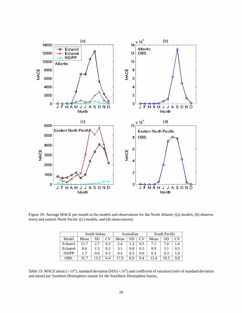
Figure 19: Average MACE per month in the models and observations for the North Atlantic ((a) models, (b) observa-tions) and eastern North Pacific ((c) models, and (d) observations).

South Indian Australian South PacificModel Mean SD CV Mean SD CV Mean SD CV

Echam3 11.7 2.7 0.2 2.4 1.3 0.5 7.1 7.0 1.0Echam4 8.6 1.5 0.2 3.1 0.8 0.3 8.9 3.1 0.3NSIPP 1.7 0.6 0.3 0.5 0.3 0.6 0.3 0.3 1.0OBS. 31.7 13.2 0.4 17.9 6.9 0.4 13.4 10.5 0.8

Table 13: MACE mean (×104), standard deviation (SD) (×104) and coefficient of variation (ratio of standard deviationand mean) per Southern Hemisphere season for the Sourthern Hemisphere basins.

29

Figure 20: Average MACE per month in the models and observations for the Australian basin ((a) models, (b) obser-vations), South Indian Ocean ((c) models, and (d) observations), and South Pacific ((e) models, (f) observations).

30


Table 14: Correlations of MACE density of models and observations: globe (GL), Northern Hemisphere (NH), andSouthern Hemisphere (SH). Bold entries indicate correlation values which have significance at the95% confidencelevel.


Table 15: Mean square error of MACE density in models and observations: globe (GL), Northern Hemisphere (NH),and Southern Hemisphere (SH).

are likely to fall near the bottom of the scale in MACE density, and therefore are colored white. This explains whythe NSIPP MACE density pattern is much less filled than the track density pattern. Also, many regions over land thatshowed up in the track density have a weaker contribution in the MACE density, such as the Australian region. Theseparation between the observed MACE patterns in the Northern and Southern Hemispheres is more evident, whilethe models’ MACE patterns remain continuous through the equator, especially in the case of Echam4 over the Pacific.

The correspondences of the model MACE density patterns with that observed are given in Tables 14 and 15, wherethe spatial correlation and the mean square error are shown, respectively. The Kolmogorov-Smirnov test comparingtwo distributions was also performed, with similar results (not shown). The Echam4 model has the highest correlationcoefficients and lowest mean square error for MACE density globally and per hemisphere. The MACE density patternof Echam4 and NSIPP in the Southern Hemisphere is more similar to the observed pattern than in the NorthernHemisphere. All models have lower mean square error and higher correlations coefficients in the Southern Hemispherethan in the Northern Hemisphere, partly due to the artificial factor of there being less tropical cyclone activity in theSouthern Hemisphere.

b. MACE interannual variability

Fig. 22 shows the MACE in the western North Pacific and South Indian Ocean in the models (ensemble mean MACE)and observations per year and Southern Hemisphere season, respectively. The model with the highest MACE values inthe western North Pacific is Echam4, and in the South Indian Ocean is Echam3. NSIPP has the lowest MACE valuesin both cases.

We performed a bias correction in the models’ MACE, similar to the one described in the models’ number of tropi-cal cyclones, such that the models have the same MACE distribution in each basin as the observed MACE distribution.The interannual variability of the bias corrected MACE in the western North Pacific and South Indian Ocean is givenin Fig. 23.

In Fig. 24 the bias corrected MACE spread of the ensemble members in each model is shown. For each model,some years the spread among the ensemble members is large, while in others the spread is very small. When the spreadis small, greater confidence of the model’s MACE response to the forcing SST may be suggested. For the Echam4model, in most years the observed MACE is within the spread of the bias corrected ensemble members, while forEcham3 and NSIPP in many years this does not occur. This may be partly a result of the Echam4’s greater number ofensemble members. Although none of the models ensemble members’ captured the observed record MACE in 1997,a few of the Echam3 ensemble members are near to the observed MACE values.

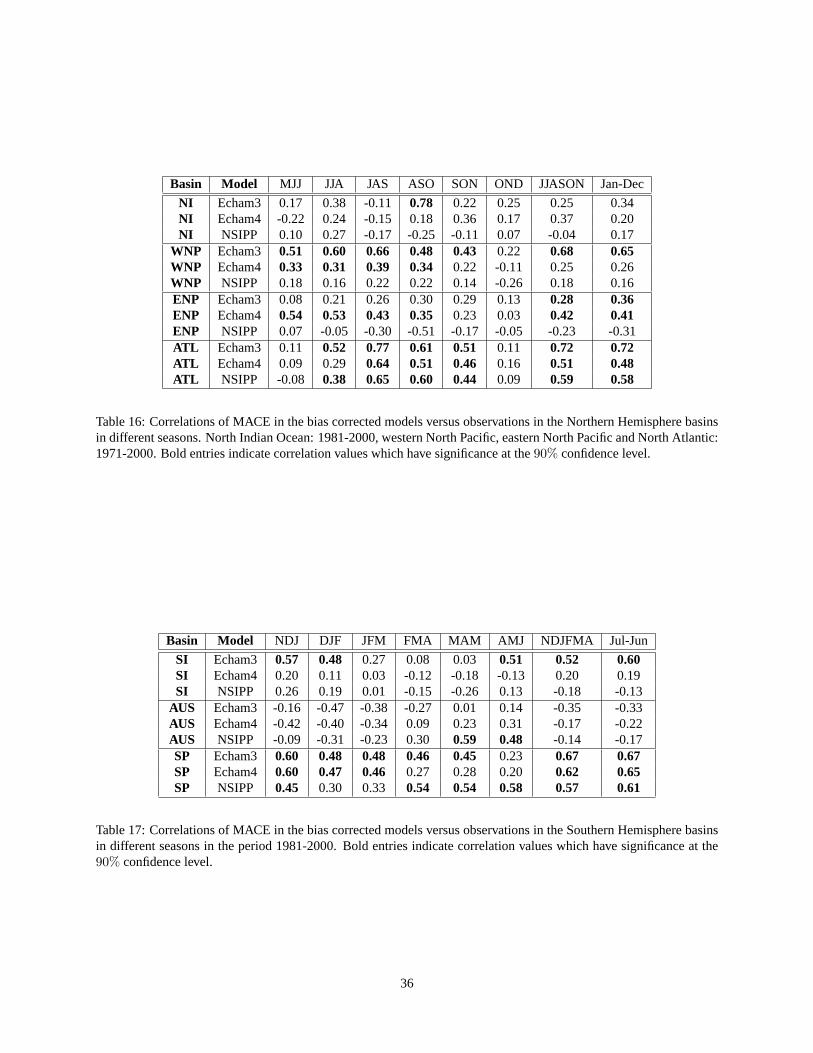
The models’ skill for MACE was calculated using correlations (see Tables 16 and 17) and additional skill measures,as shown for some basins in Figs. 26,25,28. The skill of all models in the Atlantic is relatively high. Other basinswith significant skill in the relevant seasons are western North Pacific (Echam3 and Echam4), eastern North Pacific(Echam4), and South Pacific (all models).

31

Figure 21: MACE density (in10−4m2/s2 units) in the models (a) Echam3, (b) Echam4, (c) NSIPP, and (d) observa-tions, for the period 1981-2000.

32

Figure 22: MACE per year (season) in models (ensemble mean) and observations in the western North Pacific (a) andSouth Indian Ocean (b).

33

Figure 23: Bias corrected MACE per year (season) in models (ensemble mean) and observations in western NorthPacific (a) and South Indian Ocean (b).

34

Figure 24: The models’ bias corrected MACE per year (ensemble mean and interensemble spread), and observedMACE in the western North Pacific: (a) Echam3, (b) Echam4, and (c) NSIPP.

35


NI Echam3 0.17 0.38 -0.11 0.78 0.22 0.25 0.25 0.34NI Echam4 -0.22 0.24 -0.15 0.18 0.36 0.17 0.37 0.20NI NSIPP 0.10 0.27 -0.17 -0.25 -0.11 0.07 -0.04 0.17

WNP Echam3 0.51 0.60 0.66 0.48 0.43 0.22 0.68 0.65WNP Echam4 0.33 0.31 0.39 0.34 0.22 -0.11 0.25 0.26WNP NSIPP 0.18 0.16 0.22 0.22 0.14 -0.26 0.18 0.16ENP Echam3 0.08 0.21 0.26 0.30 0.29 0.13 0.28 0.36ENP Echam4 0.54 0.53 0.43 0.35 0.23 0.03 0.42 0.41ENP NSIPP 0.07 -0.05 -0.30 -0.51 -0.17 -0.05 -0.23 -0.31ATL Echam3 0.11 0.52 0.77 0.61 0.51 0.11 0.72 0.72ATL Echam4 0.09 0.29 0.64 0.51 0.46 0.16 0.51 0.48ATL NSIPP -0.08 0.38 0.65 0.60 0.44 0.09 0.59 0.58

Table 16: Correlations of MACE in the bias corrected models versus observations in the Northern Hemisphere basinsin different seasons. North Indian Ocean: 1981-2000, western North Pacific, eastern North Pacific and North Atlantic:1971-2000. Bold entries indicate correlation values which have significance at the90% confidence level.


SI Echam3 0.57 0.48 0.27 0.08 0.03 0.51 0.52 0.60SI Echam4 0.20 0.11 0.03 -0.12 -0.18 -0.13 0.20 0.19SI NSIPP 0.26 0.19 0.01 -0.15 -0.26 0.13 -0.18 -0.13

AUS Echam3 -0.16 -0.47 -0.38 -0.27 0.01 0.14 -0.35 -0.33AUS Echam4 -0.42 -0.40 -0.34 0.09 0.23 0.31 -0.17 -0.22AUS NSIPP -0.09 -0.31 -0.23 0.30 0.59 0.48 -0.14 -0.17SP Echam3 0.60 0.48 0.48 0.46 0.45 0.23 0.67 0.67SP Echam4 0.60 0.47 0.46 0.27 0.28 0.20 0.62 0.65SP NSIPP 0.45 0.30 0.33 0.54 0.54 0.58 0.57 0.61

Table 17: Correlations of MACE in the bias corrected models versus observations in the Southern Hemisphere basinsin different seasons in the period 1981-2000. Bold entries indicate correlation values which have significance at the90% confidence level.

36

GL % NH % SH %Echam3 294.6 81% 215.4 59% 189.7 52%Echam4 330.1 90% 267.7 73% 172.4 47%NSIPP 200.3 55% 120.5 33% 98.7 27%OBS. 294.3 81% 200.0 55% 128.2 35%

Table 18: Average number of days with tropical cyclone activity in the globe (GL), Northern Hemisphere (NH)and Southern Hemisphere (SH), and the percentage of days in a year with tropical cyclone activity in models andobservations in the period 1961-2000

Fig. 25 shows the MACE skill of the three models in the western North Pacific. Both Echam3 and Echam4 havesignificant skill in the western North Pacific in most seasons, including the peak typhoon season (ASO). The skill issmaller in the later part of the year (SON and OND) in the three models.

Fig. 26 shows the MACE skill of the three models in the South Pacific. The correlation is significant in theEcham3 and Echam4 models during the tropical cyclone peak season months (January - March, JFM), but the skill isnot significant in the other measures used. The highest skills are observed for the total season (July-June) using theEcham3 model.

The MACE skill of the models in the eastern North Pacific is shown in Fig. 27. Both Echam3 and Echam4 havesignificant skill most of the year, with skill values of the Echam3 model higher than Echam4. The NSIPP model onlyhas significant skill in the early season (MJJ).

In the Atlantic, the three models have significant skill for MACE, as shown in Fig. 28. In the three models themaximum skill occurs early in the season (July to September, JAS) and diminishes later in the year. The highest skillsof all models for MACE occur in the Atlantic basin.

7. Number of Days with Tropical Cyclone Activity

When analysing how active a hurricane season is, one of the indices commonly used is the number of days withtropical cyclone activity. The number of tropical cyclones does not give any information on how strong or how long-lasting the tropical cyclones are. On the other hand, ACE (here MACE) can be strongly dominated by a handful ofvery intense tropical cyclones. Therefore to have a more complete idea of the level of activity in one season, anotherinteresting variable to analyze in the models and observations is the number of days with tropical cyclone activity. Wecount a day with tropical cyclone activity if during that day in the domain considered (global, Northern and SouthernHemispheres, and basins) a tropical cyclone is active.

The average number of days with tropical cylone activity in the globe, northern and Southern Hemispheres forthe models and observations are given in Table 18. The percentage of average number of days per year with tropicalcyclone activity is also shown in Table 18. Globally, the Echam3 average number of days with tropical cyclone activityis very similar to the observed number, while Echam4 has an excess of days and the NSIPP model not enough days.In observations, there are more days with tropical cyclone activity in the Northern Hemisphere than in the SouthernHemisphere and all models reproduce this feature. However, both Echam3 and Echam4 have more days with tropicalcyclone activity in each Hemisphere than observed, and NSIPP fewer days.

Tables 19 and 20 show the average number of days with tropical cyclone activity per basin in the models andobservations in the Northern and Southern Hemisphere, respectively. All models lack days with tropical cyclonesactivity in the North Indian ocean, with Echam4 being closest to the observed value. The NSIPP model does not haveenough tropical cyclone days in any basin, with values closest to the observed ones in the western North Pacific andthe South Indian Ocean. Echam4, and to a slight extent Echam3, have too many days with tropical cyclone activityin the western North Pacific. In the eastern North Pacific, all models lack enough days, with Echam4 having the mostactivity in that basin. The Echam3 is the only model with a realistic number of days with tropical cyclone activity inthe Atlantic, the other 2 models having almost no days.

In the Southern Hemisphere, the Echam3 and Echam4 models have varying degrees of an excess of days with trop-ical cyclone activity in the South Indian Ocean and South Pacific, contrasting with a lack of activity in the Australianbasin. Most of the days with tropical cyclone activity in the NSIPP model occurs in the South Indian Ocean, wherethe average number of days is nearly as high as the observed number.

37

Figure 25: Simulation skill of MACE in the western North Pacific for the models: (a) Echam3, (b) Echam4, and (c)NSIPP, 1971-2000. Significant skill in any of the measures is indicated with a red asterisk (∗); The circle (◦) is for thecorrelation (Corr.), the diamond (3) is for the rank correlation (R.C.), the triangle (4) is for Sommer’s Delta and thesquare (2) is for Kendall’s Tau.

NI WNP ENP ATLEcham3 13.9 4% 169.5 46% 33.6 9% 62.6 17%Echam4 34.6 9% 248.0 68% 47.8 13% 9.9 3%NSIPP 6.5 2% 110.4 30% 5.3 1% 6.5 2%OBS. 42.2 12% 150.8 41% 72.4 20% 59.2 16%

Table 19: Average number of days with tropical cyclone activity in the Northern Hemisphere basins (North Indian -NI, western North Pacific - WNP, eastern North Pacific - ENP and Atlantic - ATL), and the percentage of days in ayear with tropical cyclone activity in models and observations in the period 1961-2000

38

Figure 26: Simulation skill of MACE in the South Pacific for the models: (a) Echam3, (b) Echam4 (c) NSIPP, 1971-2000. Significant skill in any of the measures are indicated with a red asterisk (∗); The circle (◦) is for the correlation(Corr.), the diamond (3) is for the rank correlation (R.C.), the triangle (4) is for Sommer’s Delta and the square (2)is for Kendall’s Tau.

South Indian Australian South PacificEcham3 138.8 38% 31.3 9% 55.1 15%Echam4 97.7 27% 42.9 12% 83.9 23%NSIPP 69.0 19% 31.0 8% 11.6 3%OBS. 82.8 23% 56.1 15% 36.1 10%

Table 20: Average number of days with tropical cyclone activity in the Southern Hemisphere basins, and the percentageof days in a year with activity in models and observations, in the period 1961-2000

39

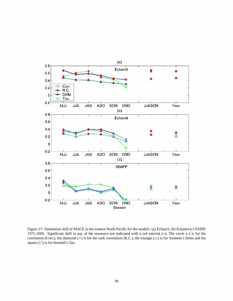
Figure 27: Simulation skill of MACE in the eastern North Pacific for the models: (a) Echam3, (b) Echam4 (c) NSIPP,1971-2000. Significant skill in any of the measures are indicated with a red asterisk (∗); The circle (◦) is for thecorrelation (Corr.), the diamond (3) is for the rank correlation (R.C.), the triangle (4) is for Sommer’s Delta and thesquare (2) is for Kendall’s Tau.

40

Figure 28: Simulation skill of MACE in the Atlantic for the models: (a) Echam3, (b) Echam4 (c) NSIPP, 1971-2000.Significant skill in any of the measures are indicated with a red asterisk (∗); The circle (◦) is for the correlation (Corr.),the diamond (3) is for the rank correlation (R.C.), the triangle (4) is for Sommer’s Delta and the square (2) is forKendall’s Tau.

41


NI Echam3 -0.19 -0.18 -0.21 -0.18 -0.41 0.12 -0.34 -0.23NI Echam4 -0.15 -0.01 -0.16 -0.08 -0.14 0.06 0.03 -0.08NI NSIPP 0.10 -0.03 -0.18 -0.05 -0.15 -0.12 0.02 0.01

WNP Echam3 0.50 0.47 0.39 0.36 0.28 0.28 0.51 0.61WNP Echam4 0.47 0.46 0.40 0.26 0.21 0.14 0.27 0.46WNP NSIPP 0.41 0.23 0.17 -0.01 -0.04 -0.38 0.18 0.26ENP Echam3 0.25 0.23 0.13 0.21 0.15 0.10 0.18 0.29ENP Echam4 0.45 0.38 0.21 0.26 0.23 0.12 0.31 0.30ENP NSIPP 0.05 -0.08 -0.41 -0.58 -0.34 -0.17 -0.35 -0.29ATL Echam3 -0.03 0.37 0.72 0.52 0.31 0.03 0.63 0.60ATL Echam4 -0.13 0.21 0.37 0.46 0.46 0.18 0.49 0.43ATL NSIPP 0.13 0.31 0.60 0.59 0.45 0.24 0.52 0.47

Table 21: Correlations of number of days with tropical cyclone activity in the bias corrected models and observationsin the Northern Hemisphere basins (North Indian Ocean - NI, western North Pacific - WNP, eastern North Pacific -ENP and Atlantic - ATL) for different seasons in the period 1971-2000. Bold entries indicate correlation values whichhave significance at the95% confidence level.

Figs. 29 and 30 show the average number of days with tropical cyclone activity per month in each basin of theNorthern and Southern Hemispheres, respectively. As was the case for other variables, none of the models reproducethe annual cycle of the number of tropical cyclone days in the North Indian Ocean. In observations, there are twomaxima–one in May and one in November–while the models generally have most of the tropical cyclone days inbetween these months. In the western North Pacific, both Echam3 and Echam4 have too many tropical cyclone days inthe off-peak months of January to June. From July to November, Echam4 still has a slight excess of days with tropicalcyclone activity, while both Echam3 and NSIPP have deficits. The NSIPP model, and to a lesser extent Echam3,peak too late in the year. While the Echam3 reproduces quite well the peak in the number of tropical cyclone daysin the Atlantic, with a small excess during the months of May to July, Echam4 has a severe deficiency of active daysthroughout the year and a late peak. The NSIPP model is also severely deficient, but has realistic seasonal phasing.

In the Southern Hemisphere, the mean number of tropical cyclone days per month of the NSIPP is much moresimilar to that observed than in the Northern Hemisphere (see Fig. 30). In the South Indian Ocean, the Echam4 hasan annual cycle for mean number of tropical cyclone days very similar to that observed (Fig. 30(a)). In contrast, theEcham3 model has a second peak in August to October that is not present in the observations. The NSIPP model has asomewhat late peak. All models do not have enough tropical cyclone days throughout the year in the Australian basin,the Echam4 having an annual cycle most similar to that observed (Fig. 30(b)). Echam4 has too many tropical cyclonedays in the South Pacific throughout the year, contrasting with the Echam3’s more realistic behavior and the NSIPPmodel’s lack of tropical cyclone days in that basin (Fig. 30(c)).

In Fig. 31 the average number of tropical cyclone days per year in the western North Pacific and the Atlantic isshown for the models and observations. In both basins there is large interannual variability in the number of tropicalcyclone days per year. The models seem to capture part of this interannual variability in these basins. The correlationsof the ensemble mean number of tropical cyclone days per year of the models with the observations is given inTables 21 (Northern Hemisphere) and 22 (Southern Hemisphere). The basins in which the models show some skill inthe relevant tropical cyclone season, using correlations and other skill measures are, the western North Pacific, Atlanticand South Pacific. The skill plots for the case of the western North Pacific and Atlantic are given in Figs. 32 and 33.

8. Life Span

It is interesting to know if the models are able to reproduce the average life span of the observed tropical cyclones. Inthis section we analyze the average life span of tropical cyclones in the models and compare with observations.

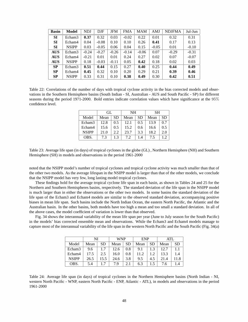
Table 23 shows the average and the standard deviation of the life span of tropical cyclones globally and in eachHemisphere. The three models’ average tropical cyclone life span is larger than the observed life span, globally andper Hemisphere. The model with the largest average life span is the NSIPP model. In the previous sections, it was

42

Figure 29: Mean number of days with tropical cyclone activity per month in the models and observations: (a) NorthIndian Ocean, (b) western North Pacific, (c) eastern North Pacific, and (d) Atlantic, in the period 1961-2000.

43

Figure 30: Mean number of days with tropical cyclone activity per month in the models and observations: (a) SouthIndian Ocean, (b) Australian region, and (c) South Pacific, in the period 1961-2000.

44

Figure 31: Mean number of days with tropical cyclone activity per year in the bias corrected models and observations:(a) western North Pacific and (b) Atlantic in the period 1961-2000.

45

Figure 32: Simulation skill of the mean number of tropical cyclone days in the western North Pacific for the models:(a) Echam3, (b) Echam4 (c) NSIPP, 1971-2000. Significant skill in any of the measures are marked with a red asterisk(∗); The circle (◦) is for the correlation (Corr.), the diamond (3) is for the rank correlation (R.C.), the triangle (4) isfor Sommer’s Delta and the square (2) is for Kendall’s Tau.

46

Figure 33: Simulation skill of the mean number of tropical cyclone days in the Atlantic for the models: (a) Echam3, (b)Echam4 (c) NSIPP, 1971-2000. Significant skill in any of the measures are marked with a red asterisk (∗); The circle(◦) is for the correlation (Corr.), the diamond (3) is for the rank correlation (R.C.), the triangle (4) is for Sommer’sDelta and the square (2) is for Kendall’s Tau.

47


SI Echam3 0.37 0.32 0.03 -0.02 0.22 0.01 0.32 0.31SI Echam4 0.04 -0.08 0.10 0.10 0.26 0.41 0.17 0.13SI NSIPP 0.03 -0.05 0.06 0.04 0.15 -0.05 0.01 -0.10

AUS Echam3 -0.24 -0.27 -0.26 -0.14 -0.06 0.07 -0.29 -0.31AUS Echam4 -0.21 0.01 0.01 0.24 0.27 0.02 0.07 -0.07AUS NSIPP 0.18 -0.03 -0.11 0.05 0.42 0.18 0.02 0.03SP Echam3 0.51 0.44 0.15 0.27 0.40 0.25 0.44 0.49SP Echam4 0.45 0.32 0.10 0.20 0.29 0.21 0.39 0.46SP NSIPP 0.33 0.31 0.10 0.38 0.49 0.30 0.42 0.51

Table 22: Correlations of the number of days with tropical cyclone activity in the bias corrected models and obser-vations in the Southern Hemisphere basins (South Indian - SI, Australian - AUS and South Pacific - SP) for differentseasons during the period 1971-2000. Bold entries indicate correlation values which have significance at the95%confidence level.

GL NH SHModel Mean SD Mean SD Mean SD

Echam3 12.8 0.5 12.1 0.5 13.9 0.7Echam4 15.6 0.5 15.2 0.6 16.6 0.5NSIPP 21.0 2.2 23.7 3.3 18.2 2.0OBS. 7.3 1.3 7.2 1.4 7.5 1.2

Table 23: Average life span (in days) of tropical cyclones in the globe (GL) , Northern Hemisphere (NH) and SouthernHemisphere (SH) in models and observations in the period 1961-2000

noted that the NSIPP model’s number of tropical cyclones and tropical cyclone activity was much smaller than that ofthe other two models. As the average lifespan in the NSIPP model is larger than that of the other models, we concludethat the NSIPP model has very few, long lasting model tropical cyclones.

These findings hold for the average tropical cyclone life span in each basin, as shown in Tables 24 and 25 for theNorthern and Southern Hemispheres basins, respectively. The standard deviation of the life span in the NSIPP modelis much larger than in either the observations or the other two models. In some basins the standard deviation of thelife span of the Echam3 and Echam4 models are similar to the observed standard deviation, accompanying positivebiases in mean life span. Such basins include the North Indian Ocean, the eastern North Pacific, the Atlantic and theAustralian basin. In the other basins, both models have too high a mean and too small a standard deviation. In all ofthe above cases, the model coefficient of variation is lower than that observed.

Fig. 34 shows the interannual variability of the mean life span per year (June to July season for the South Pacific)in the models’ bias corrected ensemble mean and observations. While the Echam3 and Echam4 models manage tocapture most of the interannual variability of the life span in the western North Pacific and the South Pacific (Fig. 34(a)

NI WNP ENP ATLModel Mean SD Mean SD Mean SD Mean SD

Echam3 9.6 1.7 12.6 0.8 9.1 1.3 12.7 1.1Echam4 17.5 2.5 16.0 0.8 11.2 1.2 13.3 1.4NSIPP 26.5 15.5 24.6 3.8 9.5 4.5 21.4 11.8OBS. 5.4 1.7 7.9 2.1 6.3 1.5 7.6 1.4

Table 24: Average life span (in days) of tropical cyclones in the Northern Hemisphere basins (North Indian - NI,western North Pacific - WNP, eastern North Pacific - ENP, Atlantic - ATL), in models and observations in the period1961-2000

48

SI AUS SPModel Mean SD Mean SD Mean SD

Echam3 14.5 0.6 14.7 1.9 11.0 1.6Echam4 16.5 0.9 19.1 1.4 15.2 1.0NSIPP 20.0 3.6 15.2 2.5 12.7 3.5OBS. 8.2 1.8 7.4 2.0 6.5 2.1

Table 25: Average life span (in days) of tropical cyclones in the Southern Hemisphere basins, in models and observa-tions in the period 1961-2000


NI Echam3 0.10 0.18 0.03 -0.20 0.02 -0.08 0.01 -0.07NI Echam4 -0.13 0.01 -0.20 -0.02 -0.30 -0.17 0.16 0.26NI NSIPP 0.35 0.18 -0.08 -0.05 0.04 -0.29 -0.03 0.17

WNP Echam3 0.25 0.45 0.51 0.45 0.50 0.51 0.61 0.65WNP Echam4 0.34 0.60 0.65 0.48 0.57 0.58 0.65 0.63WNP NSIPP 0.16 -0.11 -0.09 -0.37 -0.30 -0.39 -0.36 -0.20ENP Echam3 0.35 0.19 0.12 0.24 0.12 0.01 0.10 0.11ENP Echam4 -0.02 0.17 0.20 0.00 0.06 0.28 0.10 0.20ENP NSIPP 0.24 -0.31 -0.49 -0.44 -0.12 -0.11 -0.16 -0.12ATL Echam3 -0.07 -0.03 0.20 0.19 0.17 0.14 0.06 0.05ATL Echam4 0.04 -0.14 0.05 0.35 0.32 0.01 0.25 0.24ATL NSIPP 0.22 0.06 0.07 0.10 -0.05 -0.05 0.13 0.11

Table 26: Correlations of the bias corrected mean life span of tropical cyclones in the models and observations in theNorthern Hemisphere basins (North Indian - NI, western North Pacific - WNP, eastern North Pacific - ENP, Atlantic- ATL), in different seasons in the period 1971-2000. Bold entries indicate correlation values which have significanceat the95% confidence level.

and (b)), this does not occur in the Atlantic (Fig. 34(c)).These conclusions are supported by the correlations of the mean life span per year between the models and the

observations shown in Tables 26 and 27, for the Northern and Southern Hemisphere basins, respectively. The onlybasins in which the models have significant skill for average life span in the relevant seasons are the western NorthPacific (Echam3 and Echam4) and the South Pacific (Echam4).

9. Model tropical cyclone categories

Due to the low-resolution, the models’ tropical cyclones are considerably weaker than observed tropical cyclones. Inorder to analyze the typical strengths of the model tropical cyclones, we show in Table 28 the mean and maximumwind speed of all model and observed tropical cyclones. Table 29 shows the maximum wind speed of each basin inthe models and observations.

The mean tropical cyclone wind speed in the models is on the order of half of the mean wind speed of the observa-tions, globally and per Hemisphere. The maximum model tropical cyclone wind speed for the globe is aproximatelyone third of the maximum global wind speed in the observations. The tropical cyclone wind speed distribution in themodels has a bias proportional to that of the mean wind speed. However, the models’ tropical cyclone winds speeddistribution has smaller positive skewness than the observed distribution, being more symetric about the mean value.The long tail of the observed tropical cyclone wind speed distribution corresponds to very intense tropical cyclonesthat are absent in the models.

The observed tropical cyclone wind speed distribution mean and maximum is larger in the Northern than theSouthern Hemisphere. In the case of the mean wind speed, both Echam4 and NSIPP have larger values in the NorthernHemisphere than the Southern Hemisphere, while for the maximum this occurs in Echam3 and Echam4. However,in all cases, the ratio between the Northern and Southern Hemisphere is much larger in the observations than in the

49

Figure 34: Bias corrected mean life span (in days) in the models and observations: (a) South Pacific (per season), (b)western North Pacific (per year) and (c) Atlantic (per year), in the period 1961-2000.

50


SI Echam3 0.01 0.46 0.32 0.29 -0.10 0.17 0.24 0.11SI Echam4 -0.07 -0.19 -0.18 -0.24 0.10 -0.16 -0.36 -0.35SI NSIPP 0.02 -0.14 -0.19 -0.36 -0.09 -0.25 -0.36 -0.34

AUS Echam3 0.12 0.14 0.15 0.30 0.12 -0.13 0.38 0.26AUS Echam4 0.00 0.22 -0.05 -0.17 0.15 0.12 0.02 0.03AUS NSIPP -0.17 -0.11 -0.33 -0.29 0.17 0.32 -0.32 -0.34SP Echam3 -0.06 0.02 -0.21 0.01 0.15 0.42 -0.12 0.04SP Echam4 -0.08 0.05 -0.03 -0.07 -0.05 0.32 0.42 0.42SP NSIPP -0.24 -0.33 -0.29 -0.04 0.00 -0.11 -0.51 -0.52

Table 27: Correlations of the bias corrected average life span of tropical cyclones in models and observations in theSouthern Hemisphere basins (South Indian - SI, Australian - AUS, South Pacific - SP) in different seasons during theperiod 1971-2000. Bold entries indicate correlation values which have significance at the95% confidence level.

Model Mean Wind Speed Maximum Wind Speed

Globe NH SH Globe NH SHEcham3 12.7 12.6 12.8 35.7 35.7 31.0Echam4 13.3 13.3 13.3 35.6 35.6 32.8NSIPP 12.9 13.3 12.1 27.5 26.3 27.5Obs. 25.6 26.5 22.8 95.2 95.2 77.2

Table 28: Mean and maximum wind speed (inm/s) in the globe, Northern Hemisphere (NH) and Southern Hemi-sphere (SH) in the models and observations, in the period 1981-2000.

models.In observations, the basin with highest maximum wind speed is the western North Pacific. Echam3 and Echam4

reproduce this feature. In observations, the basin with lowest mean tropical cyclone wind speed is the North IndianOcean, a result reproduced by Echam3. Echam4’s lowest mean tropical cyclone wind speed occurs in the easternPacific. In the case of the NSIPP model this occurs in the Australian basin, which interestingly is where this modelalso reaches the maximum value of tropical cyclone wind speed.

A percentile-based bias correction in the model wind speed distribution is performed, similar to the bias correctionsperformed for other variables. However, the wind speed distribution of models and observations are very distinct, asshown in Fig. 35, with the observations having a much more skewed distribution than the models. This implies thatthe models’ highest percentiles have very similar values, in contrast to the observed values where, for example, the95th percentile would have a much higher value than the 90th percentile.

After the correction, we use the observed Dvorak scale to define the intensity of each storm. We then categorize themodels’ tropical cyclones as tropical depressions, tropical storms, hurricanes and intense hurricanes and compare thepercentage frequencies with those of the observations. In Camargo and Zebiak (2002) the definition of the thresholds

SI AUS SP NI WNP ENP ATLEcham3 28.8 29.9 31.0 19.8 35.7 32.7 32.5Echam4 28.3 31.3 32.9 23.1 35.6 34.4 31.6NSIPP 22.3 27.5 27.3 20.5 26.3 25.8 26.0Obs. 77.2 72.0 74.6 72.0 95.2 82.3 84.9

Table 29: Maximum wind speed (inm/s) in the different basins (South Indian - SI, Australian - AUS, South Pacific -SP, western North Pacific - WNP, eastern North Pacific - ENP, Atlantic - ATL) in the models and observations in theperiods 1981-2000 (SI, AUS, SP and NI) and 1961-2000 (WNP, ENP, ATL).

51

Figure 35: Wind speed (inm/s) distribution of all model tropical cyclones )a) Echam3, (b) Echam4, (c) NSIPP and(d) observed tropical cyclones, which reach at least tropical storm strength in the western North Pacific in the period1961-2000.

52

Model GlobeTD % TD TS % TS H % H IH % IH

Echam3 1.3 2.5 % 11.5 22.6 % 17.3 33.9 % 20.9 41.0 %Echam4 0.6 1.2% 8.4 17.4 % 16.5 34.0 % 22.9 47.4 %NSIPP 0.2 1.4% 2.2 13.5 % 6.7 40.5 % 7.3 44.6 %Obs. 0 0% 38.4 43.7 % 26.2 30.0 % 22.8 26.2 %

Table 30: Average global number of tropical cyclones with tropical depression (TD), tropical storm (TS), hurricane(H) and intense hurricane (IH) strength and relative percentage in each category in the models and observations. Forthe observations, only tropical cyclones with at least tropical storm strength were considered.

Model Northern Hemisphere Southern HemisphereTS % TS H % H IH % IH TS % TS H % H IH % IH

Echam3 6.7 13.1% 8.8 17.3% 13.6 26.5 % 4.8 9.4 % 8.5 16.6 % 7.4 14.4 %Echam4 4.9 10.2% 9.7 20.1% 16.6 34.4 % 3.4 7.1 % 6.8 14.0 % 6.3 12.9 %NSIPP 0.8 5.2% 2.5 15.3% 4.9 29.8 % 1.4 8.3 % 4.1 25.2 % 2.4 14.8 %Obs. 25.0 28.6% 18.3 20.9% 16.6 18.9 % 12.9 14.8 % 7.9 9.0 % 6.3 7.2 %

Table 31: Average number of tropical cyclones with tropical storm (TS), hurricane (H) and intense hurricane (IH)strength and relative percentage in each category from the global total, in the models and observations.

for wind speed, vorticity and temperature such that a model vortex could be defined as a tropical cyclone was based inthe statistical distribution of these fields. We assumed that these model tropical cyclones would have at least tropicalstorm strength, and compared with comparable data from observations. Here, we can check to see if this assumptionwas valid for the models, by categorizing the model tropical cyclones and verifying the percentage of these whichwould fall in the tropical depression category.

Because some of the earlier data on the observed tropical cyclones in the Southern Hemisphere and North IndianOcean do not have wind speed data, we only use data in the period 1981-2000. For consistency, we restrict our analysesto this period for the globe and the hemispheres.

Tables 30 and 31 show the average number of tropical cyclones per year, with tropical storms, hurricane andintense hurricane strength globally and per Hemisphere, respectivelly. Also shown in these tables is the correspondingpercentage of these tropical storms, hurricane and intense hurricane strength to the total number of named tropicalstorms (observations) and model tropical cyclones.

By correcting the model wind speed distribution prior to obtaining the number of tropical cyclones in each strengthcategory, we obtain a plausible distribution. However, the number of tropical cyclones was not corrected, so thedeficiency of the overall numbers is evident also in the frequencies by strength category (Tables 30 and 31). Ofgreater interest, however, is the percentage frequency of each tropical cyclone strength of the global total number oftropical cyclones. From Table 30 one can see that the percentage of tropical depressions globally in the models isapproximately 2% of the total. Therefore, the assumption that the models’ tropical cyclones are of tropical stormstrength or higher appears justified.

The models tend to have a lower percentage of tropical storm strength tropical cyclones than the observations,globally, in each Hemisphere (Tables 30 and 31), and by basin (Fig. 36). Approximately 80% of the model tropicalcyclones have the strength of either hurricane or intense hurricane, while in observations only slightly more than halfof the named tropical cyclones have these two highest strength categoreies. The percentage of tropical storm strengthtropical cyclones in the models is approximately half of the observed percentage, globally and per Hemisphere. BothEcham3 and Echam4 reproduce this feature, while NSIPP has more tropical cyclones with all strengths in the SouthernHemisphere. In the Northern Hemisphere, all models have more tropical cyclones with intense hurricane strengththan with hurricane strength, which is not the case in observations. In the Southern Hemisphere, both Echam3 andEcham4 have more tropical cyclones with hurricane strength than with intense hurricane strength, in analogy to theobservations; however, the percentages of the global total of these categories are too high.

In all basins and models there is a tendency toward a bias of having too few model tropical cyclones with tropical

53

Basin Model NDJFMA July-June

TS HUR IHUR TS HUR IHURSI Echam3 0.19 0.18 0.49 -0.27 0.46 0.54SI Echam4 -0.19 0.09 0.34 -0.33 0.28 0.35SI NSIPP 0.03 -0.35 0.03 -0.01 -0.28 -0.03

AUS Echam3 -0.30 -0.45 -0.22 -0.32 -0.39 -0.25AUS Echam4 0.24 0.15 0.23 0.21 0.12 0.16AUS NSIPP 0.36 -0.07 -0.05 0.16 -0.11 -0.14SP Echam3 0.20 0.75 0.60 0.37 0.76 0.63SP Echam4 0.39 0.70 0.44 0.47 0.72 0.52SP NSIPP 0.36 0.69 0.06 0.53 0.66 0.07

Table 32: Correlations of interannual variability of the number of model tropical cyclones and observations with dif-ferent strengths in the Southern Hemisphere basins in the period 1981/1982-1999/2000 for NDJFMA and the SouthernHemisphere July-June season. Bold entries indicate correlation values which have significance at the95% confidencelevel.

storm strength and too many with hurricane and intense hurricane strength (Fig. 36). The extent to which these per-centages differ from the observed percentage is dependent on the model and the basin. In some basins, the percentageof tropical cyclones with hurricane strength is very similar to the observed, such as the South Pacific, western NorthPacific and Atlantic, while in others, the difference is huge, i.e. the Australian basin. The same is true for the othertropical cyclone strengths.

We analyzed the skill of the models in simulating the interannual variability of the number of model tropicalcyclones with tropical storm, hurricane and intense hurricane strength. The skill levels are in general lower than forthe total number of model tropical cyclones. From the three intensities analysed (tropical storm, hurricane and intensehurricanes), the one with least skill in all models is that of tropical storm. In the basins in which there are significantskill levels, the highest skills occur for the intense hurricane and/or hurricane strengths. In Figs. 37, 38, 39, the skillof the models’ Atlantic tropical cyclones with tropical storm, hurricane and intense hurricane strengths, respectively,are shown. Note that in the Atlantic hurricane peak season (ASO - August to October), no models have significantskill in the number of tropical storms, while Echam3 and Echam4 have significant skill in that season for hurricaneand intense hurricane strength.

Tables 33 and 32 show correlations of the number of tropical cyclones with different strengths in the SouthernHemisphere and Northern Hemisphere basins, respectively. Note that in the South Indian Ocean, where the Echam3model has no skill in the total number of model tropical cyclones (Table 9), there is significant skill for the higherintensity cyclones. This is in contrast with the Australian basin, where Echam4 has significant skill for the totalnumber of tropical cyclones (Table 9) and no significant skill when the number of tropical cyclones with differentstrengths are considered. In the Southern Hemisphere, as was the case for the number of tropical cyclones, the highestskills occur in the South Pacific basin, especially for all models’ tropical cyclones with hurricane intensity. Note thatfor the total number of tropical cyclones in the Southern Hemisphre 40 years of data were being used, while here only20 years are considered, for reasons explained above.

In the Northern Hemisphere the only basins with significant skill for model tropical cyclones with hurricane and/orintense hurricane strengths are the western North Pacific (Echam3 and Echam4) and the Atlantic (all models). As inthe number of tropical cyclones, the highest skill scores occur in the Atlantic, especially using the Echam3 model.

The fact that the models have least skill for the number of tropical storms may be related to the relative deficit ofthe models’ tropical storms, as compared to their hurricanes or intense hurricanes. Our conclusion is that the AGCMsin this low resolution cannot simulate the gradations of tropical cyclone strength with much realism.

10. Tracks Centroid

Another interesting aspect that we would like to study is to what extent the model tracks are in the correct location,and also whether year-to-year shifts in the tracks location are reproduced in the models. In this section we analyze theinterannual variation of the tracks centroid, which is defined as the average latitude and longitude of tropical cyclone

54

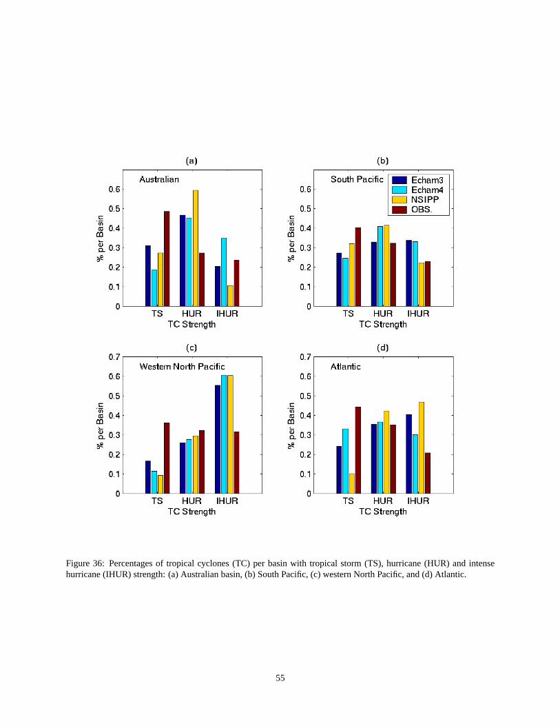
Figure 36: Percentages of tropical cyclones (TC) per basin with tropical storm (TS), hurricane (HUR) and intensehurricane (IHUR) strength: (a) Australian basin, (b) South Pacific, (c) western North Pacific, and (d) Atlantic.

55

Figure 37: Simulation skill for interannual variability of the number of tropical cyclone with tropical storm strengthin the Atlantic for the models: (a) Echam3, (b) Echam4 (c) NSIPP, for 1971-2000. Significant skill in any of themeasures are marked with a red asterisk (∗); The circle (◦) is for the correlation (Corr.), the diamond (3) is for therank correlation (R.C.), the triangle (4) is for Sommer’s Delta and the square (2) is for Kendall’s Tau.

56

Figure 38: Simulation skill for interannual variability of the number of tropical cyclones with hurricane strength inthe Atlantic for the models: (a) Echam3, (b) Echam4, and (c) NSIPP, for 1971-2000. Significant skill in any of themeasures are marked with a red asterisk (∗); The circle (◦) is for the correlation (Corr.), the diamond (3) is for therank correlation (R.C.), the triangle (4) is for Sommer’s Delta and the square (2) is for Kendall’s Tau.

57

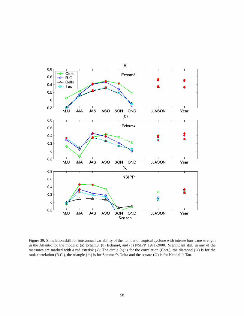
Figure 39: Simulation skill for interannual variability of the number of tropical cyclone with intense hurricane strengthin the Atlantic for the models: (a) Echam3, (b) Echam4, and (c) NSIPP, 1971-2000. Significant skill in any of themeasures are marked with a red asterisk (∗); The circle (◦) is for the correlation (Corr.), the diamond (3) is for therank correlation (R.C.), the triangle (4) is for Sommer’s Delta and the square (2) is for Kendall’s Tau.

58

Basin Model JJASON Year

TS HUR IHUR TS HUR IHURNI Echam3 -0.01 -0.05 -0.19 0.03 0.12 -0.01NI Echam4 -0.16 0.17 0.24 -0.17 0.27 0.01NI NSIPP 0.27 -0.03 0.08 0.20 0.03 0.09

WNP Echam3 -0.33 0.37 0.41 -0.31 0.43 0.48WNP Echam4 -0.21 0.28 -0.24 -0.24 0.44 -0.16WNP NSIPP 0.01 0.24 0.02 0.12 0.28 -0.06ENP Echam3 -0.03 0.30 0.29 0.06 0.32 0.36ENP Echam4 0.22 0.35 0.33 0.21 0.34 0.29ENP NSIPP -0.16 -0.30 0.02 -0.21 -0.30 0.06ATL Echam3 0.05 0.56 0.55 -0.01 0.59 0.52ATL Echam4 0.38 0.52 0.40 0.39 0.49 0.46ATL NSIPP 0.03 0.38 0.26 0.04 0.35 0.29

Table 33: Correlations of interannual variability of the number of model tropical cyclones and observations withdifferent strengths in the Northern Hemisphere basins in the period 1971-2000 for JJASON and year. Bold entriesindicate correlation values which have significance at the95% confidence level.

North Indian Western North Pacific Eastern North Pacific North AtlanticModel Latitude Longitude Latitude Longitude Latitude Longitude Latitude LongitudeEcham3 11.2N 81.5E 16.9N 155.5E 15.8N 131.7W 19.5N 49.0WEcham4 14.9N 81.3E 16.3N 154.2E 14.6N 122.5W 15.1N 78.5WNSIPP 5.2N 86.2E 13.3N 122.6E 12.7N 108.1W 14.1N 89.5WObs. 15.4N 80.9E 18.8N 135.9E 17.3N 119.1W 24.5N 67.7W

Table 34: Average latitude and average longitude of all tracks per basin in the Northern Hemisphere in the period1961-2000.

location in the period considered. Table 34 shows the average latitude and longitude in the Northern Hemispherebasins over the period of 1961-2000. The average latitude in the models in all basins is nearer the equator than inobservations, especially in the Atlantic. The average longitude in the North Indian Ocean of Echam3 and Echam4 isvery smilar to the observed average longitude. In contrast, in the western North Pacific, both Echam3 and Echam4have the previously noted bias to the east, while the NSIPP has a slight bias to the west. The average longitude in theeastern North Pacific is very similar to the observed in the Echam4, while Echam3 has a bias to the west and NSIPP abias to the east. In the Atlantic, Echam3 has a bias to the east, while Echam4 has a slight westerly bias and NSIPP astronger westerly bias.

In the Southern Hemisphere, for most of the basins and models the average latitude of the tracks in the periodJuly 1961 - June 2000 is closer to the equator compared with the observed mean latitude. In the South Indian Ocean,the mean longitude of the NSIPP model is very near the observed one, while Echam3 and Echam4 have a bias tothe east. The NSIPP model has also the average longitude closest to the observed in the Australian basin, with theEcham4 having a large bias towards the east related to deficient tropical cyclone activity near the Autralian west coast.Similarly to the western North Pacific, in the South Pacific both Echam3 and Echam4 have a bias to the west, whilethe NSIPP average longitude is to the east of the observed average longitude.

In some basins, such as the western North Pacific, the centroid has a well defined annual cycle (see Fig. 40). Theaverage latitude in the western North Pacific reaches its most northerly value in August, with the most equatorwardposition occuring in February (see Fig. 41). Though the models’ bias in the centroid longitude is very clear (Fig. 40),all models nonetheless capture the average latitude annual cycle quite well, especially Echam4. Though the annualcycle of the latitude in the NSIPP model has the correct general shape, the equatorward bias is very pronounced.

The interannual variability of the mean latitude and longitude is very different from basin to basin. Some basinshave a much larger interannual variability than others. In Figs. 42 and 43 the mean latitude and longitude per year

59

South Indian Australian South PacificModel Latitude Longitude Latitude Longitude Latitude LongitudeEcham3 12.7S 77.8E 15.7S 141.6E 21.0S 172.6WEcham4 13.0S 74.0E 13.6S 151.5E 18.5S 174.8WNSIPP 10.5S 67.9E 9.6S 134.6E 16.0S 177.5EObs. 16.6S 69.0E 16.9S 137.3E 19.4S 179.7W

Table 35: Average latitude and average longitude of all tracks per basin in the Southern Hemisphere in the period1961/1962 - 1999/2000.

Figure 40: Average latitude and longitude per month in the western North Pacific (a) Echam3, (b) Echam4, (c) NSIPP,and (d) observations.

60

Figure 41: Average latitude per month in the western North Pacific in the models and observations.

or Southern Hemisphere season is shown for the western North Pacific and Australian basin, respectively. In theAustralian basin there is a much larger standard deviation for the mean longitude (6.7) than the mean latitude (2.8),while in the the North Indian Ocean the standard deviation in latitude and longitude are similar (2.6 and 2.9).

The models have a reasonable interannual variability for the average latitude in the western North Pacific (Fig. 42(a))with the mean equatorward latitude bias in all models as already discussed. The interannual variabiltiy of the meanlongitude in the western North Pacific is shown in (Fig. 42(b)), with the known eastward bias for Echam3 and Echam4and westward bias for NSIPP clearly seen.

In the Australian basin, NSIPP has a larger interannual variability than the observations and the other two models(Fig. 43(a)). The mean longitude variability of the Echam4 model is too small and with a large bias to the east(Fig. 43(b)). This results from this model having most of the Australian tropical cyclones near the east coast andvery few near the Australian west coast. This does not occur in the other two models (Echam3 and NSIPP), whoseinterannual variabilities are more similar to that observed.

In tables 36-39 the correlations of the centroid latitude and longitude of the models with observations are given.It is important to note that in the years that a model (or the observations) do not produce any tropical cyclones forthe given season, there are no values of latitude and longitude to be used in the correlations. In such a case, thatyear is excluded from the correlation for the particular season, and the significances tests are made more strict toaccommodate the smaller sample size.

In tables 36 and 37, the correlations of the centroid latitude in models and observations are given for the Southernand Northern Hemispheres basins, respectively. In the South Pacific basin, all models have high and significant skillfor the centroid latitude. The Echam4 model has also significant skill for the centroid latitude in the Australian basin.In the Northern Hemisphere, both Echam3 and Echam4 have significant skill for the centroid latitude mainly for thewestern North Pacific. The Echam4 also has significant skill for the centroid latitude in the North Indian Ocean inOND, while the NSIPP model has significant skill in the eastern North Pacific in JAS, both cases being the peaktropical cyclone season in that basin.

Tables 38 and 39 show the correlations of the centroid longitude in models and observations for the Southern andNorthern Hemispheres basins, respectively. The correlations values for longitude are weaker than those for latitude.In the Southern Hemisphere, the only basin with significant correlations for the centroid longitude is the South Pacific,especially in the late season (AMJ) and for the three models. In the Northern Hemisphere, significant correlations forthe centroid longitude appear in the western North Pacific, for all models, but in different seasons, with all models

61

Figure 42: Average latitude (a) and longitude (b) per year in the western North Pacific in the models and observationin the period 1961-2000.

62

Figure 43: Average latitude (a) and longitude (b) per year in the Australian basin in the models and observations in theperiod 1961/1962-1999/2000.

63


SI Echam3 -0.17 0.24 -0.03 0.12 -0.01 0.10 -0.05 -0.03SI Echam4 0.07 -0.05 -0.08 0.11 0.05 0.04 0.11 0.25SI NSIPP -0.29 -0.12 -0.08 -0.19 -0.37 0.05 -0.01 0.06

AUS Echam3 0.04 -0.03 0.10 0.13 0.23 -0.01 0.04 0.11AUS Echam4 0.26 0.37 0.30 0.27 0.42 0.20 0.47 0.60AUS NSIPP 0.01 -0.16 -0.01 0.03 0.20 -0.19 -0.18 -0.03SP Echam3 0.43 0.42 0.50 0.44 0.42 0.31 0.52 0.58SP Echam4 0.78 0.86 0.83 0.80 0.51 0.01 0.90 0.90SP NSIPP 0.50 0.66 0.70 0.64 -0.12 -0.33 0.72 0.65

Table 36: Correlations for the interannual variability of the average latitude of tropical cyclone tracks in the modelsand observations in the Southern Hemisphere basins in their respective seasons in the period 1971/1972 - 1999/2000.In each case only years with a total number of tropical cyclones different from zero in that season in models andobservations are included in the correlation. Bold entries indicate correlation values which have significance at the95% confidence level.


NI Echam3 0.30 0.03 -0.04 -0.36 -0.01 -0.22 -0.16 -0.27NI Echam4 -0.05 -0.06 -0.43 -0.24 0.16 0.51 -0.09 -0.08NI NSIPP -0.16 -0.26 -0.16 -0.02 0.01 0.05 -0.36 -0.29

WNP Echam3 0.21 0.61 0.56 0.39 0.07 0.10 0.36 0.54WNP Echam4 0.50 0.68 0.70 0.43 0.11 0.21 0.54 0.56WNP NSIPP 0.16 0.13 -0.19 -0.40 -0.14 -0.09 -0.51 -0.54ENP Echam3 0.10 0.26 -0.14 -0.09 0.07 0.19 -0.03 -0.01ENP Echam4 0.14 0.20 0.11 -0.10 0.07 0.15 -0.01 0.02ENP NSIPP 0.00 0.36 0.79 0.13 0.25 0.20 0.17 0.14ATL Echam3 0.02 0.18 0.06 0.13 -0.24 -0.31 0.09 0.13ATL Echam4 -0.24 -0.23 -0.49 -0.43 -0.32 -0.31 -0.38 -0.29ATL NSIPP 0.23 0.14 -0.04 -0.16 -0.30 0.01 -0.45 0.07

Table 37: Correlations for the interannual variability of the average latitude of tropical cyclone tracks in the modelsand observations in the Northern Hemisphere basins in their respective seasons in the period 1971-2000. In each caseonly years with a total number of tropical cyclones different from zero in that season in models and observations areincluded in the correlation. Bold entries indicate correlation values which have significance at the95% confidencelevel.

64


SI Echam3 0.03 -0.09 -0.17 -0.01 0.09 -0.17 -0.03 0.12SI Echam4 -0.23 -0.26 -0.34 0.12 0.05 -0.35 -0.18 -0.08SI NSIPP -0.01 -0.14 -0.35 0.07 0.11 -0.42 -0.28 -0.19

AUS Echam3 0.23 0.09 0.23 0.13 0.20 0.00 0.25 0.19AUS Echam4 0.16 0.12 0.16 0.07 0.33 0.19 0.14 0.21AUS NSIPP 0.13 -0.05 0.05 -0.15 0.20 0.26 0.14 0.20SP Echam3 0.20 -0.02 0.07 0.27 0.39 0.53 0.31 0.30SP Echam4 0.41 0.16 0.25 0.35 0.44 0.53 0.35 0.34SP NSIPP -0.16 -0.09 -0.11 0.22 0.14 0.52 0.13 0.15

Table 38: Correlations for the interannual variability of the average longitude of tropical cyclones tracks in the modelsand observations in the Southern Hemisphere basins in different seasons in the period 1971/1972 - 1999/2000. In eachcase only years with a total number of tropical cyclones different from zero in that season in models and observationsare included in the correlation. Bold entries indicate correlation values which have significance at the95% confidencelevel.

having significant skill for JJASON and the whole year. Other significant correlations for the centroid longitude appearin the North Indian Ocean (Echam4, JJASON) and eastern North Pacific (Echam3 and Echam4, JAS).

11. Season Peak

Another feature that we would like to know if the models can reproduce is which month the tropical cyclone seasonis most active and if the models are able to simulate the interannual shifts that occur in the timing. In this section, thetiming of the season peak in each basin is calculated using as weight either the number of tropical cyclones in eachmonth or MACE for each month. The resulting month number generally contains a fractional component; for example,8.4 would refer to very late August, 8.8 would be early-to-middle September, and 9.0 would be mid-September.

Tables 40 and 41 show the month number of the average of the temporal distribution based on both the number oftropical cyclones (NTC) and tropical cyclone activity (MACE), in the period 1961-2000, for the Northern Hemispherebasins or July 1961 to June 2000 for the Southern Hemisphere basins (in the case of MACE, the 1981-2000 period isused).

In table 40, we show that in the North Indian basin, all models have a tendency to peak earlier in the year thanthe observations. This reflects the annual cycle being centered in the summer in the models, instead a double seasonwith a smaller peak in the spring and a larger peak in the fall. In the western North Pacific, both Echam3 and Echam4peak earlier in the year (around July), than the observations, which peaks in August. The NSIPP models peaks inSeptember. In the eastern North Pacific the peak season happens around August in both models and observations. Inthe Atlantic, all models and observations peak between August and September. There is little difference in the resultsas a function of whether the temporal centroid is calculated from the number of tropical cyclones or the tropical cyloneactivity; the MACE tends to have just slightly later resultthan the NTC, in models and observations.

Table 41 shows that the average peak month in the South Indian Ocean in the Echam3 happens near December,while in the observations and Echam4 and NSIPP the peak month occurs between January and February. In theobservations the peak month in the Australian basin is around February, which is reproduced by Echam4, whileEcham3 and NSIPP have slightly early peaks. Finally, in the South Pacific, peak month happens between January andFebruary in the observations, nearer February if MACE is considered. Echam3 peak in the South Pacific is very nearthe observed peak, with Echam4 peak slightly later than the observed (nearer February) and NSIPP slightly earlier(nearer January). Overall the models have very little bias in the mean peak month compared with biases in othervariables analysed previously. The exception occurs in the North Indian Ocean, where, as mentioned earlier, all themodels fail to reproduce the bimodal annual cycle and therefore peak too early.

Fig. 44 shows the interannual variability of the season peak (NTC weighted) in the western North Pacific. ThoughEcham3 and Echam4 have an an early bias, they nonetheless reproduce some of the features of the season peak in thatbasin. NSIPP has a late bias and a much larger range of values for the season peak than either the observations or theother two models.

65


NI Echam3 0.21 0.30 0.07 -0.08 0.08 -0.21 0.02 0.00NI Echam4 -0.33 -0.01 -0.04 0.11 -0.13 0.06 0.45 0.29NI NSIPP 0.01 -0.33 -0.54 -0.17 -0.05 -0.22 0.04 -0.10

WNP Echam3 -0.08 -0.04 0.10 0.35 0.57 0.63 0.38 0.40WNP Echam4 0.35 0.20 0.18 0.39 0.61 0.79 0.51 0.67WNP NSIPP 0.18 0.16 0.09 0.43 0.46 0.32 0.51 0.48ENP Echam3 0.15 0.25 0.43 0.29 0.12 -0.14 0.43 0.48ENP Echam4 -0.18 0.33 0.36 0.32 -0.03 -0.22 0.34 0.31ENP NSIPP 0.00 -0.22 -0.32 -0.15 -0.34 -0.23 -0.17 -0.16ATL Echam3 -0.12 0.06 0.19 0.29 0.15 -0.59 0.32 0.28ATL Echam4 -0.07 0.14 0.24 0.01 -0.12 -0.08 0.08 0.05ATL NSIPP -0.56 -0.19 -0.07 -0.10 -0.17 -0.23 -0.05 -0.02

Table 39: Correlations for the interannual variability of the average longitude of tropical cyclones tracks in the modelsand observations in the Northern Hemisphere basins in different seasons in the period 1971-2000. In each case onlyyears with a total number of tropical cyclones different from zero in that season in models and observations areincluded in the correlation. Bold entries indicate correlation values which have significance at the95% confidencelevel.

North Indian Western North Pacific Eastern North Pacific North AtlanticModel NTC MACE NTC MACE NTC MACE NTC MACE

M SD M SD M SD M SD M SD M SD M SD M SDEcham3 7.7 1.0 7.8 1.0 7.2 0.7 7.3 0.8 8.2 0.9 8.3 0.7 8.1 0.2 8.1 0.3Echam4 7.4 0.4 7.6 0.4 7.5 0.6 7.6 0.6 8.4 0.6 8.5 0.6 8.5 0.5 8.6 0.5NSIPP 6.7 1.5 7.8 1.3 9.1 0.8 9.6 0.8 8.6 2.5 8.9 2.0 8.8 1.9 8.9 1.9OBS. 8.7 1.3 9.0 1.9 8.2 0.5 8.6 0.5 8.0 0.3 8.1 0.3 8.6 0.4 8.8 0.4

Table 40: Mean (M) and standard deviation (SD) of the season peak month number based on the number of tropicalcyclones (NTC) and the tropical cyclone activity (MACE) in the Northern Hemisphere basins in the period 1961-2000and 1981-2000 (North Indian MACE).

South Indian Australian South PacificModel NTC MACE NTC MACE NTC MACE

M SD M SD M SD M SD M SD M SDEcham3 11.8 0.7 12.1 0.6 1.1 1.0 1.0 0.7 1.5 0.6 1.6 0.7Echam4 1.1 0.6 1.3 0.6 1.7 0.5 1.9 0.6 1.8 0.4 2.2 0.4NSIPP 1.4 1.0 1.6 1.0 12.9 1.1 12.8 1.0 1.3 1.1 1.4 1.1OBS. 1.3 0.6 1.9 0.6 1.8 0.4 2.0 0.9 1.5 0.8 1.7 1.6

Table 41: Average and standard deviation of the season peak month number based on the number of tropical cy-clones (NTC) and the tropical cyclone activity (MACE) in the Southern Hemisphere basins in the period 1961/1962 -1999/2000 (NTC) and 1981/1982 - 1999/2000 (MACE).

66

Figure 44: Season peak in the models and observations in western North Pacific 1961-2000.

Table 42 shows the correlations for the interannual variations between the models and observations of the seasonpeak based on the number of tropical cyclones (NTC) and the tropical cyclone activity (MACE). The only model withsignificant skill for the season peak is the Echam4 model in the western North Pacific (NTC and MACE), easternNorth Pacific (MACE) and South Indian (NTC).

12. Conclusions

In this report, we analysed the main properties of tropical cyclones in three low-resolution AGCMs. The main aim ofthis report is to study the climatology and seasonal skill of the AGCMs’ tropical cyclones. Despite the low resolution,the models do have significant skill in some tropical cyclone properties on seasonal scales. The skill is model andbasin dependent and also varies with the tropical cyclone characteristic analyzed. We cannot point to a single modelas having a best skill in the different tropical cyclone variables globally.

In all models, the tropical cyclone activity occurs nearer the equator than in observations. One region in which allmodels have low skill is the Indian Ocean, both south and north of the equator. In the North Indian Ocean even thetropical cyclone activity annual cycle is poorly simulated by the three models. In number of tropical cyclones, the twobasins where all models have significant skill is the South Pacific and the Atlantic. This is probably due to the strongrelation to ENSO in these two basins, as will be further discussed in Camargo et al. (2004). The Atlantic and westernNorth Pacific stand out as the basins, where in most variables the models’s have significant skills.

Though the models’ tropical cyclones are much weaker than observed ones, the models’ MACE indices havesignificant skills in some basins when compared to the observed MACE indices. In the eastern North Pacific, forinstance, the Echam4 model does not have significant skill in the peak season (JAS) for the number of tropical cyclones,but has significant skill in that season for the ACE index. The opposite happens in this model for the Australian region.

Overall, Echam4 is the model with most significant skills in the different properties, especially in the westernNorth Pacific and the South Pacific. Echam3 has in general better skill in the Atlantic than the other models. NSIPPhas very different characteristics in the Southern and Northern Hemispheres, being more similar to observations in theSouthern Hemisphere. Though NSIPP has a slightly higher numerical resolution than both Echam models, this did

67

Echam3 Echam4 NSIPPBasin NTC MACE NTC MACE NTC MACE

NI -0.10 0.02 -0.23 0.07 -0.06 0.04WNP 0.32 0.22 0.62 0.45 0.26 0.19ENP 0.02 -0.15 0.32 0.54 0.02 0.15ATL -0.21 -0.12 -0.02 0.07 0.13 0.23SI 0.31 0.18 0.52 0.24 0.34 0.04

AUS 0.03 0.04 0.03 -0.12 0.25 0.17SP 0.21 -0.32 0.21 -0.11 0.09 0.04

Table 42: Correlations of the year-to-year variations of season peak between models and observations, based onnumber of tropical cyclones (NTC) and tropical cyclone activity (MACE). The correlations using NTC are in theperiod 1971-2000 (Northern Hemisphere basins), and 1971/1972 - 1999/2000 (Southern Hemisphere basins). Thecorrelations using MACE are in the period 1971-2000 (western North Pacific, eastern North Pacific and Atlantic),1981-2000 (North Indian) and 1981/1982-1999/2000 (Southern Hemisphere basins). Bold entries indicate correlationvalues which have significance at the95% confidence level.

not guarantee in better tropical cyclone activity characteristics, as other factors have significant importance such asphysical parametrization schemes, as discussed in Vitart and Stockdale (2001). For some attributes, such as the firstposition density pattern, the NSIPP model has better skill than the other two models.

The Echam3 and Echam4 models have very long tracks in the Southern Hemisphere compared to the observations,and this is reflected as too long life spans in these models. Though the NSIPP model’s tropical cyclones has shortertracks in the Southern Hemisphere, the life spans of this model are even longer, reflecting the characteristic of thetropical cyclones in this model very slow movement. The Echam3 and Echam4 models have some skill in the interan-nual variability of the tropical cyclones’ life span in the Western North Pacific, but in the other Northern Hemispheresbasins there are no significant skills.

An attempt was made to classify the models’ tropical cyclones in the strength categories and divide them in tropicalstorm, hurricane and intense hurricane. The number of tropical cyclones in each category was then counted. Thereare fewer skillful basins in this case than when all the categories were considered together. This is due to the low-horizontal resolution of the models which leads to a distribution of wind speed with a much smaller positive tail thanthe observed one, which makes distinction among the strenght categories difficult without loosing skill.

In summary, some aspects of the observed tropical cyclone activity are being nicely reproduced by the models,while others have significantly greater problems. In the companion paper (see Camargo et al. (2004)), we analyze indetail how the tropical cyclone characteristics and skills are influenced by and related to ENSO.

68

13. Appendix - Definition Intra-ensemble, External and Total Variances

Following Li (1999) and references therein, any variable is defined asx(n, y), wheren represents the ensemblemember withN = 10 being the total number of ensemble members, andy represents the year withY = 17 being thetotal number of years considered. We can then define two averages: the ensemble mean and the climatological mean.The ensemble mean is defined with the respect to the integration member in the ensemble:

xe(y) =1N

N∑n=1

x(n, y). (1)

The climatological mean is taken to respect to the integrations and years:

xc =1

NY

N∑n=1

Y∑y=1

x(n, y) =1Y

Y∑y=1

xe(y). (2)

The interannual variability signal can be described by the yearly variation of the ensemble meanxe(y) about theclimatological mean:

σ2e =

1Y

Y∑y=1

[xe(y)− xc]2. (3)

The varianceσ2e then measures the external, or forced signal. On the other hand, the dispersion within the ensemble

members can be defined as:

σ2i =

1Y

Y∑y=1

[1N

N∑n=1

[x(n, y)− xe(y)]2]

, (4)

which measures the internal model variability. Finally, the total variance is the sum of the internal and the externalvariance:

σ2t =

1NY

N∑n=1

Y∑y=1

[x(n, y)− xc]2 = σ2

e + σ2i . (5)

Acknowledgement The authors would like to thank Dr. Marx Suarez and Michael Kistler (NSIPP) for making theNSIPP model data available for this project. We would also like to thank Max-Planck Institute for Meteorology(Hamburg, Germany) for making both versions of their model Echam accessible to IRI. The first author (SJC) thanksDr. Simon Mason (IRI) for suggestions on statistical measures. Discussions with of these results with Dr. Adam H.Sobel (Columbia University), Dr. Lisa Goddard (IRI) and Dr. Simon Mason (IRI) are acknowleged. We thank Dr. M.Benno Blumenthal (IRI) for the IRI data library.

69

Bibliography

Arpe, K., L. Dumenil, and M. Giorgetta, 1998: Variability of the Indian Monsoon in the ECHAM3 Model: Sensitivityto Sea Surface Temperature, Soil Moisture and the Stratospheric Quasi-Biennial Oscillation.J. Clim., 11, 1837–1858.

Avila, L., R. J. Pasch, J. L. Beven, J. L. Franklin, M. B. Lawrence, S. R. Stewart, and J. Jiing, 2003: Eastern NorthPacific hurricane season of 2001.Mon. Wea. Rev., 131, 249–262.

Barnston, A. G., S. J. Mason, L. Goddard, D. G. DeWitt, and S. Zebiak, 2003: Multimodel ensembling in seasonalclimate forecasting at IRI.Bull. Amer. Meteor. Soc., 84, 1783–1796.

Bell, G. D., M. S. Halpert, R. C. Schnell, R. W. Higgins, J. Lawrimore, V. E. Kousky, R. Tinker, W. Thiaw, M. Chelliah,and A. Artusa, 2000: Climate assessment for 1999.Bull. Amer. Meteor. Soc., 81, S1–S50.

Bengtsson, L., 2001: Hurricane threats.Science, 293, 440–441.

Bengtsson, L., H. Bottger, and M. Kanamitsu, 1982: Simulation of hurricane-type vortices in a general circulationmodel.Tellus, 34, 440–457.

Bengtsson, L., M. Botzet, and M. Esh, 1995: Hurricane-type vortices in a general circulation model.Tellus, 47A,175–196.

—, 1996: Will greenhouse gas-induced warming over the next 50 years lead to higher frequency and greater intensityof hurricanes?Tellus, 48A, 57–73.

Broccoli, A. J. and S. Manabe, 1990: Can existing climate models be used to study anthropogenic changes in tropicalcyclone climate?Geophys. Rev. Lett., 17, 1917–1920.

Camargo, S. J., A. G. Barnston, and S. E. Zebiak, 2004: Tropical Cyclones in Atmospheric General CirculationModels, Part II: ENSO Influence, in preparation.

Camargo, S. J., H. Li, and L. Sun, 2002: Simulation of typhoons in the regional spectral model.Abstracts of the 4thInternational RSM Workhsop, Los Alamos, NM, 7.

Camargo, S. J. and A. H. Sobel, 2004: Formation of tropical storms in an atmospheric general circulation model.Tellus A, 56, 56–67.

Camargo, S. J. and S. E. Zebiak, 2002: Improving the detection and tracking of tropical storms in Atmospheric GeneralCirculation Models.Wea. Forecasting, 17, 1152–1162.

Chan, J. C. L., J. E. Shi, and C. M. Lam, 1998: Seasonal forecasting of tropical cyclone activity over the WesternNorth Pacific and the South China Sea.Wea. Forecasting, 13, 997–1004.

Cherchi, A. and A. Navarra, 2003: Reproducibility and predictability of the Asian summer monsoon in the ECHAM4-GCM. Clim. Dyn., 20, 365–379.

CPC, 2004: Available on line at http://www.cpc.noaa.gov/products/.

Franklin, J. L., L. A. Avila, J. L. Beven, M. B. Lawrence, R. J. Pasch, and S. R. Stewart, 2003: Eastern North Pacifichurricane season of 2002.Mon. Wea. Rev., 131, 2379–2393.

70

Goddard, L., A. G. Barnston, and S. J. Mason, 2003: Evaluation of the IRI’s “Net Assessment” seasonal climateforecasts: 1997-2001.Bull. Amer. Meteor. Soc., 84, 1761–1781.

Goddard, L., S. J. Mason, S. E. Zebiak, C. F. Ropelewski, R. E. Basher, and M. A. Cane, 2001: Current approaches toseasonal to interannual climate predictions.Int. J. Climatol., 21, 1111–1152.

Gray, W. M., C. W. Landsea, P. W. M. Jr., and K. J. Berry, 1993: Predicting Atlantic basin seasonal tropical cycloneactivity by 1 August.Wea. Forecasting, 8, 73–86.

—, 1994: Predicting Atlantic Basin Seasonal Tropical Cyclone Activity by 1 June.Wea. Forecasting, 9, 103–115.

Haarsma, R. J., J. F. B. Mitchell, and C. A. Senior, 1993: Tropical disturbances in a GCM.Clim. Dyn., 8, 247–257.

IRI, 2004: IRI (International Research Institute for Climate Prediction) Typhoon Activity Forecasts. available on lineat: http://iri.columbia.edu/forecast/typhoon/.

JTWC, 2004: JTWC (Joint Typhoon Warning Center) best track dataset, available online athttps://metoc.npmoc.navy.mil/jtwc/besttracks/.

Krishnamurti, T. N., 1988: Some recent results on numerical weather prediction over the tropics.Aust. Meteor. Mag.,36, 141–170.

Krishnamurti, T. N., D. Oosterhof, and N. Dignon, 1989: Hurricane prediction with a high resolution global model.Mon. Wea. Rev., 117, 631–669.

Lal, M., U. Cubash, J. Perliwitz, and J. Waszewitz, 1997: Simulation of the Indian monsoon climatology in ECHAM3climate model: sensitivity to horizontal resolution.Int. J. Clim., 17, 847–858.

Landman, W. A., A. Seth, and S. J. Camargo, 2002: The effect of regional climate model domain choice on thesimulation of tropical cyclone-like vortices in the southwestern indian ocean. IRI Technical Report 02-06, 31 pp.,International Research Institute for Climate Prediction, Palisades, NY, J. Climate, under revision (January, 2004).

Li, Z. X., 1999: Ensemble atmospheric gcm simulation of climate interannual variability from 1979 to 1994.J. Cli-mate, 12, 986–1001.

Liu, K. S. and J. C. L. Chan, 2003: Climatological characteristics and seasonal forecasting of tropical cyclones makinglandfall along the South China coast.Mon. Wea. Rev., 131, 1650–1662.

Manabe, S., J. L. Holloway, and H. M. Stone, 1970: Tropical circulation in a time-integration of a global model of theatmosphere.J. Atmos. Sci., 27, 580–613.

Mason, S. J., L. Goddard, N. E. Graham, E. Yulaeva, L. Q. Sun, and P. A. Arkin, 1999: The IRI seasonal climateprediction system and the 1997/98 El Nino event.Bull. Amer. Meteor. Soc., 80, 1853–1873.

May, W. H., 2003: The Indian summer monsoon and its sensitivity to the mean SSTs: Simulations with the ECHAM4AGCM at T106 horizontal resolution.J. Meteor. Soc. Japan, 81, 57–83.

Model User Support Group, 1992: Echam3 - atmospheric general circulation model. Technical Report 6, Das DeutshesKlimarechnenzentrum, Hamburg, Germany, 184pp.

NHC, 2004: NHC (National Hurricane Center) best track dataset, available online athttp://www.nhc.noaa.gov/pastall.shtml.

Roeckner, E., K. Arpe, L. Bengtsson, M. Christoph, M. Claussen, L. Dumenil, M. Esch, M. Giorgetta, U. Schlese, andU. Schulzweida, 1996: The atmospheric general circulation model ECHAM-4: Model description and simulationof present-day climate. Technical Report 218, Max-Planck Institute for Meteorology, Hamburg, Germany, 90 pp.

Ryan, B. F., I. G. Watterson, and J. L. Evans, 1992: Tropical cyclone frequencies inferred from Gray’s yearly genesisparameter: Validation of GCM tropical climate.Geophys. Res. Lett., 19, 1831–1834.

71

Sheskin, D. J., 2000:Handbook of Parametric and Nonparametric Statistical Procedures. Chapman & Hall/CRC,Boca Raton, Florida, USA, 2nd edition.

Suarez, M. J. and L. L. Takacs, 1995: Documentation of the Aries/GEOS dynamical core Version 2. NASA TechnicalMemorandum 104606, Vol 6., Goddard Space Flight Center, Greenbelt, MD, 58 pp.

Sugi, M., A. Noda, and N. Sato, 2002: Influence of global warming on tropical cyclone climatology: An experimentwith the JMA global model.J. Meteor. Soc. Japan, 80, 249–272.

Thorncroft, C. and I. Pytharoulis, 2001: A dynamical approach to seasonal prediction of Atlantic tropical cycloneactivity. Wea. Forecasting, 16, 725–734.

TSR, 2004: Tropical Storm Risk, available online at http://tropicalstormrisk.com/.

Tsutsui, J. I. and A. Kasahara, 1996: Simulated tropical cyclones using the National Center for Atmospheric Researchcommunity climate model.J. Geophys. Res., 101, 15013–15032.

Vitart, F., D. Anderson, and T. Stockdale, 2003: Seasonal forecasting of tropical cyclone landfall over Mozambique.J. Climate, 16, 3932–3945.

Vitart, F., J. L. Anderson, and W. F. Stern, 1997: Simulation of interannual variability of tropical storm frequency inan ensemble of GCM integrations.J. Climate, 10, 745–760.

—, 1999: Impact of large-scale circulation on tropical storm frequency, intensity and location, simulated by an ensem-ble of GCM Integrations.J. Climate, 12, 3237–3254.

Vitart, F. D. and T. N. Stockdale, 2001: Seasonal forecasting of tropical storms using coupled GCM integrations.Mon.Wea. Rev., 129, 2521–2537.

Walsh, K. and B. Ryan, 2000: Tropical cyclone intensity increase near australia as a result of climate change.J.Climate, 13, 3029–3036.

Watterson, I. G., J. L. Evans, and B. F. Ryan, 1995: Seasonal and interannual variability of tropical cyclogenesis:Diagnostics from large-scale fields.J. Climate, 8, 3052–3066.

Wu, G. and N. C. Lau, 1992: A GCM Simulation of the relationship between tropical storm formation and ENSO.Mon. Wea. Rev., 120, 958–977.

72

properties of tropical cyclones in atmospheric general

Documents