Department of Economics

Economic Research Paper No. 00/2

Properties of MacroeconomicProperties of MacroeconomicForecast ErrorsForecast Errors

David I. Harvey and Paul Newbold

January 2000

Centre for International, Financial and Economics ResearchDepartment of EconomicsLoughborough UniversityLoughboroughLeics., LE11 3TUUK

Tel: + 44 (0)1509 222734Fax: + 44 (0) 1509 223910Email: E.J.Pentecost@lboro.ac.uk

Director : Dr Eric J PentecostDeputy Director : Professor C J Green

Associate Directors:

Professor Kenneth J Button, George Mason University, USA

Professor Peter Dawkins, University of Melbourne, Australia

Professor Robert A Driskill, Vanderbilt University, USA

Professor James Gaisford, University of Calgary, Canada

Professor Andre van Poeck, University of Antwerp, Belgium

Professor Amine Tarazi, University of Limoges, France

Properties of Macroeconomic Forecast Errors

DAVID I. HARVEY

Department of Economics, Loughborough University, Loughborough, Leicestershire, LE11 3TU, UK

(tel.: +44 (0)1509 222712, fax: +44 (0)1509 223910, e-mail: D.I.Harvey@Lboro.ac.uk)

and

PAUL NEWBOLD

School of Economics, University of Nottingham, University Park, Nottingham, NG7 2RD, UK

(tel.: +44 (0)115 9515392, fax: +44 (0)115 9514159, e-mail: Paul.Newbold@Nottingham.ac.uk)

ABSTRACT

This paper investigates the distributional properties of individual and consensus time series

macroeconomic forecast errors, using data from the Survey of Professional Forecasters. The

degree of autocorrelation and the presence of ARCH in the consensus errors is also

determined. We find strong evidence of leptokurtic forecast errors and some evidence of

skewness, suggesting that an assumption of error normality is inappropriate; many of the

forecast error series are found to have non-zero mean, and we find sporadic evidence of

consensus error ARCH. Properties of the distribution of cross-sectional forecast errors are

also examined.

KEY WORDS: Survey data; Forecast error distribution; Non-normality.

1

The distributional properties of economic forecast errors are important from the

perspectives of both ex ante prediction and ex post forecast evaluation. With regard to the

former, it is good practice to supplement point forecasts with an estimate of the uncertainty

associated with the prediction, especially when one considers the role of forecasting in

decision making and policy. The most common approach is to produce a (symmetric)

prediction interval around the point forecast, where the actual is predicted to lie between

certain limits with a specified probability, although recently the more general approach of

density forecasting has received more attention, involving estimation of the probability

distribution of possible outturns (see, for example, Diebold, Tay and Wallis, 1999, and Tay

and Wallis, 2000). Prediction intervals can be computed in numerous ways (see Chatfield,

1993), but the methods generally rely on some understanding or assumption of the underlying

forecast error distribution. An assumption of forecast error normality is commonplace; for

example, both the Bank of England and the National Institute of Economic and Social

Research utilise the normal distribution when generating their interval and density forecasts

of UK macroeconomic variables (Wallis, 1999; Tay and Wallis, 2000).

From the perspective of ex post forecast evaluation, forecast error distribution

properties are equally important when assumptions concerning the error distribution are

made. For example, standard tests of equal forecast accuracy and forecast encompassing

typically assume normally distributed errors. Diebold and Mariano (1995) and Harvey,

Leybourne and Newbold (1998) examine tests of these two hypotheses respectively, and

demonstrate each test’s lack of robustness when the errors are non-normal. In both cases,

alternative robust tests are proposed (Harvey, Leybourne and Newbold, 1997, also propose a

small-sample modification to the Diebold-Mariano test).

Given these considerations, it is interesting to examine the distributional characteristics

of past forecast errors, and particularly the extent to which the distributions follow or depart

from the normal distribution. Although some work has been done in this area (for example,

Zarnowitz and Braun, 1993), little has been done on the properties of individual forecasters as

opposed to the consensus forecasts, or with recent data. This paper analyses predictions from

a panel of US forecasters, taken from the Survey of Professional Forecasters, primarily using

conventional summary statistics, for both individual forecasters and the consensus (mean)

forecasts. The forecasts are of inflation, GDP growth, the short-term interest rate and the

unemployment rate over four horizons.

In addition to the investigation of distributional forecast error properties, we also

2

analyse serial dependence in the forecast error time series. The order of any autocorrelation

present in the errors is determined, and we test for the presence of forecast error

autoregressive conditional heteroskedasticity (ARCH). The latter property is also important

for the forecast evaluation tests mentioned above, as discussed by Harvey, Leybourne and

Newbold (1999b) who highlight the problematic effects of ARCH on the hypothesis tests,

and suggest alternative procedures accordingly. Due to data constraints, this serial

dependence analysis is performed only for the consensus forecast errors. Finally, we also

examine the cross-sectional properties of the forecast errors, again using summary statistics

to characterise aspects of the underlying distributions.

The paper is structured in the following way. Section 1 outlines the data employed in

the study, including detail on the Survey of Professional Forecasters. Sections 2 and 3 present

our analysis of the time series properties of the errors, for individual forecasters in the survey

and for the consensus forecasts respectively. Section 4 addresses the issue of cross-section

forecast error properties, and Section 5 concludes.

1. DATA

The data are errors from point forecasts of four US macroeconomic variables – the

percentage change in the consumer price index (CPI), the percentage change in real gross

domestic product (GDP), the 3-month Treasury bill (T-bill) rate and the civilian

unemployment rate. The percentage changes in CPI and real GDP are measured as changes

on the previous quarter, expressed as an annual percentage. For each economic variable, the

data are errors from a panel of forecasts, with predictions being made from one to four steps

ahead. Forecasts are made at quarterly intervals over the period 1981:3-1997:4, with the

exception of the unemployment rate which has earlier coverage, extending the sample to

1968:4-1997:4.

The forecasts are taken from the Survey of Professional Forecasters (SPF), which

provides a quarterly survey of a number of US macroeconomic forecasts. The survey began

in 1968 as the ASA-NBER Economic Outlook Survey, organised jointly by the American

Statistical Association and the National Bureau of Economic Research, then in 1990 changed

hands and was extended and relaunched by the Federal Reserve Bank of Philadelphia as the

SPF. The survey asks a fairly diverse range of private sector forecasters to provide point

forecasts for a variety of variables and horizons, plus density forecasts for GDP and its

deflator. There are about thirty respondents each quarter on average, and the SPF maintains a

3

policy of forecaster anonymity. Zarnowitz (1969) and Croushore (1993) provide further detail

on the survey. Much work has been done using data from the SPF, investigating a variety of

issues including forecast performance and accuracy (for example Zarnowtiz, 1984, Fair and

Shiller, 1989, and Zarnowitz and Braun, 1993), forecast rationality (for example Zarnowitz,

1985, Keane and Runkle, 1990, and Baghestani and Kianian, 1993), and forecast uncertainty

and density forecasts (for example Lahiri and Teigland, 1987, Zarnowitz and Lambros, 1987,

and Diebold, Tay and Wallis, 1999). The full SPF data set can be obtained from the

Philadelphia Federal Reserve Board website; this site also contains a more complete set of

references to work that has made use of or discussed the SPF data in some way.

Although the SPF dates back to 1968, many variables only entered the survey in 1981

(or later). We have elected to analyse the forecast errors of key macroeconomic variables

which receive most economic and political interest, thus preferring real GDP and the CPI to

nominal GDP and its price deflator respectively, even though the latter have longer samples

in the survey.

There are two peculiarities associated with the real GDP forecasts which should be

noted. First, prior to 1992, the survey reports forecasts for real gross national product (GNP).

This should have little impact on our results since the analysis solely concerns forecast errors,

which were constructed using corresponding output measures for actuals and forecasts. (For

notational convenience, here and throughout the paper we refer to these errors simply as real

GDP forecast errors.) Secondly, respondents predict the level of real GDP rather than its

percentage change. However, as well as predicting future outturns of real GDP, the

forecasters also provide predictions of its level in the current and past quarter. The percentage

change forecast made by a given forecaster can therefore be derived by comparing their h-

steps ahead prediction with their estimate of the current quarter value.

The error made by forecaster i at time t for a given variable and horizon is given by

ittit fye −= , where itf denotes the forecast and ty the corresponding actual. Actuals for the

percentage change in the CPI, the T-bill rate and the unemployment rate were all obtained

from Datastream. For the percentage change in real GDP and GNP, levels data were taken

from the Federal Reserve Bulletin, using first published (unrevised) values, then converted to

annualised percentage changes on the previous quarter accordingly.

4

2. INDIVIDUAL FORECASTER ERRORS

From the full SPF data on the four variables described above, we initially investigate

properties of individual forecasters’ predictions over time, in particular by examining

summary statistics for the forecast error time series. Although our samples range from

1968/1981 to 1997, the forecasting records of particular survey respondents are generally

much shorter; indeed some forecasters only have entries for a few surveys over that time

span. We exclude respondents for whom there are less than an arbitrarily chosen minimum

number of forecasts recorded. Clearly, a trade-off exists between the number of included

forecasters and the minimum number of observations required for inclusion. After some

experimentation, a minimum number of thirty observations seems to provide the best balance,

given the estimation requirements of our analysis.

It is important to note that we do not require the included time series to be unbroken;

consequently, the forecast error series have a number of ‘missing observations’ in this sense.

Such a feature is not problematic for estimation of the summary statistics, but does preclude

any analysis of serial dependence, for example autocorrelation and ARCH; this limitation is

addressed in the next section.

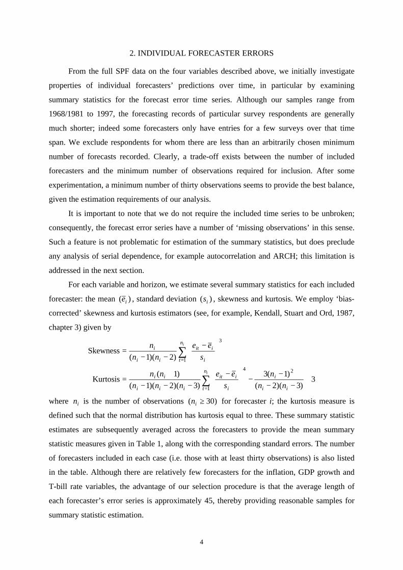
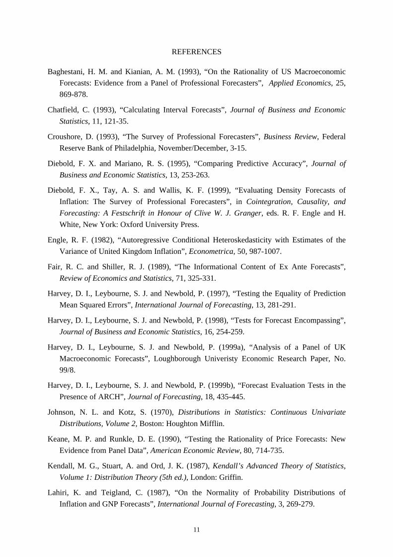
For each variable and horizon, we estimate several summary statistics for each included

forecaster: the mean )( ie , standard deviation )( is , skewness and kurtosis. We employ ‘bias-

corrected’ skewness and kurtosis estimators (see, for example, Kendall, Stuart and Ord, 1987,

chapter 3) given by

∑

∑

=

=

+−−

−−

−−−−

+=

−−−

=

i

i

n

t ii

i

i

iit

iii

ii

n

t i

iit

ii

i

nn

n

s

ee

nnn

nn

s

ee

nn

n

1

24

1

3

3)3)(2(

)1(3

)3)(2)(1(

)1(Kurtosis

)2)(1(Skewness

where in is the number of observations )30( ≥in for forecaster i; the kurtosis measure is

defined such that the normal distribution has kurtosis equal to three. These summary statistic

estimates are subsequently averaged across the forecasters to provide the mean summary

statistic measures given in Table 1, along with the corresponding standard errors. The number

of forecasters included in each case (i.e. those with at least thirty observations) is also listed

in the table. Although there are relatively few forecasters for the inflation, GDP growth and

T-bill rate variables, the advantage of our selection procedure is that the average length of

each forecaster’s error series is approximately 45, thereby providing reasonable samples for

summary statistic estimation.

5

Results for the forecast error means highlight a certain degree of bias. The percentage

change in CPI is, on average, underpredicted by 0.5% one step ahead, rising to 0.9% four

steps ahead. This is consistent with Zarnowitz and Braun (1993) who find similar behaviour

displayed in consensus forecasts of inflation, also using SPF data. It is also perhaps

unsurprising that the magnitude of the errors grows with the forecast horizon, due to the

effects of error accumulation. A similar pattern of underprediction can be observed for the T-

bill rate forecasts, although the magnitude is smaller. The error measures for the GDP growth

forecasts are also negative at each horizon, but due to larger variability, the mean summary

statistics are insignificant at the 5%-level (using an approximate significance rule of ±2

standard errors). The unemployment rate forecast errors have more mixed behaviour: one

step ahead the mean summary statistic is just less than zero and marginally significant, two

steps ahead the measure is insignificant, while the three and four steps ahead errors display

significant evidence of overprediction, albeit of a relatively minor degree (approximately

0.1%).

The means of the forecast error standard deviations are largely constant around 2-3%

for inflation and GDP growth, whereas for the T-bill rate and unemployment rate predictions,

they rise with the horizon from approximately 1% to 2% and 0.5% to 1% respectively. The

latter feature indicates that the forecast error variance may be positively related to uncertainty

at the time of prediction. It is also noticeable that the mean standard deviations for the

unemployment rate forecast errors are substantially smaller than for the other variables

considered; combining this observation with the variable’s smaller mean error measures

suggests that this series may be somewhat easier to predict.

Regarding the mean skewness measures, we find strong evidence of negative skewness

for inflation at all horizons and the T-bill rate one and two steps ahead. Equally strong

evidence exists for the unemployment rate errors being positively skewed; there is no

significant evidence of skewness for the GDP growth forecast errors. With the exception of

the real GDP errors, there is thus little support for an assumption of symmetry in the

distribution of macroeconomic forecast errors.

The mean kurtosis values given in the table are greater than three without exception.

Further, in all but two cases (T-bill rate three and four steps ahead; these results are treated as

exceptions in the following discussion), the measures are significantly greater than three,

implying strong evidence of leptokurtic forecast errors. The excess kurtosis is generally

larger for the inflation and GDP growth errors (kurtosis approximately 6.5 or more) than for

6

the T-bill rate and unemployment rate errors (kurtosis approximately 4.5), but fat-tailed

behaviour is a clear feature of these macroeconomic forecast errors.

It is also interesting to analyse the kurtosis values from another perspective. Sampling

variability enters our results not only through the averaging of the summary statistics, but

also through those statistics’ initial estimation. If we treat a given mean kurtosis value as a

kurtosis estimate derived from a series of length equal to the (rounded) mean number of

observations for that variable and horizon, an interesting question is then whether this

estimated kurtosis is significantly greater than three, thus taking account of sampling

variability in the statistic’s estimation. An approximate test of the null that this population

kurtosis is three against a one-sided alternative can be performed via Monte Carlo simulation.

The distribution of estimated kurtosis values under the null can be simulated by repeatedly

drawing a sample of m realisations from the standard normal distribution and calculating the

sample kurtosis, where m is the (rounded) mean number of observations for that variable and

horizon. Simulation in this manner (we use 10,000 replications) permits calculation of the

test’s probability values. The results of this experiment are given in Table 1 for each variable

and horizon, and reinforce the above inference, with rejections of the null occurring at least at

the 1%-level for inflation and GDP growth, the 2%-level for the T-bill rate (excepting three

and four steps ahead as before), and the 5%-level for the unemployment rate.

The leptokurtosis displayed in the series provides evidence in favour of non-normal

forecast error distributions; the most obvious alternative which admits such fat-tailed

characteristics is the Student’s t distribution. Under the assumption that the generating

distribution underlying the mean summary statistics is Student’s t, the final row of Table 1

gives the corresponding degrees of freedom that the mean kurtosis values imply. The degrees

of freedom are about five for the inflation and GDP growth errors, rising slightly for the T-

bill rate and unemployment rate errors (again with the two T-bill rate exceptions). These

values give an impression of the extent to which the forecast error distributions depart from

normality, and suggest that an assumption of normal errors in interval prediction or forecast

evaluation is misplaced. The non-normal distributions simulated in Diebold and Mariano

(1995) and Harvey, Leybourne and Newbold (1997, 1998) are Student’s t with five and six

degrees of freedom; these results provide evidence in favour of such simulations, and add

weight to these authors’ recommendation to use robust or non-parametric tests for equal

forecast accuracy and encompassing.

7

3. CONSENSUS FORECAST ERRORS

In addition to the analysis of individual forecaster performance, it is also of interest to

study the consensus forecast, defined here as the sample mean of the predictions at a

particular point in time. The consensus forecast can be thought of as a simple combined

forecast where all the available forecasts are pooled with equal weight. The consensus

forecast error, for a given variable and horizon, is therefore defined by

∑=

−=tN

iittt eNcfe

1

1

where tN is the number of available forecasts at time t. We first examine the properties of

the consensus forecast error time series by way of summary statistics as in the previous

section (obviously there is now only one summary statistic for a particular variable and

horizon, and no subsequent averaging takes place). The results are given in Table 2.

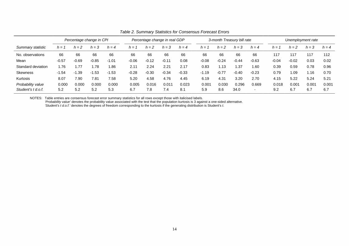
The distributional properties of the consensus errors are not dissimilar to those of the

individual forecasters analysed above. Underprediction of almost identical magnitdues is

displayed in the inflation and T-bill rate forecast errors, the unemployment rate errors are

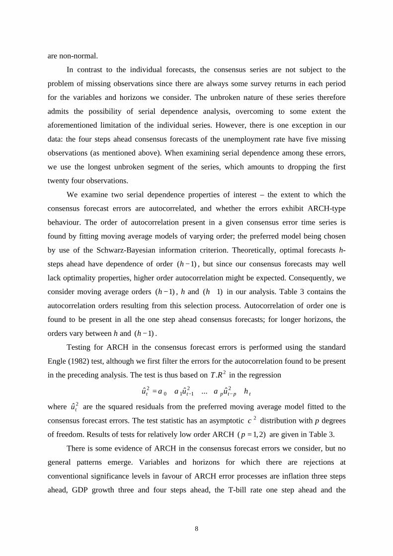
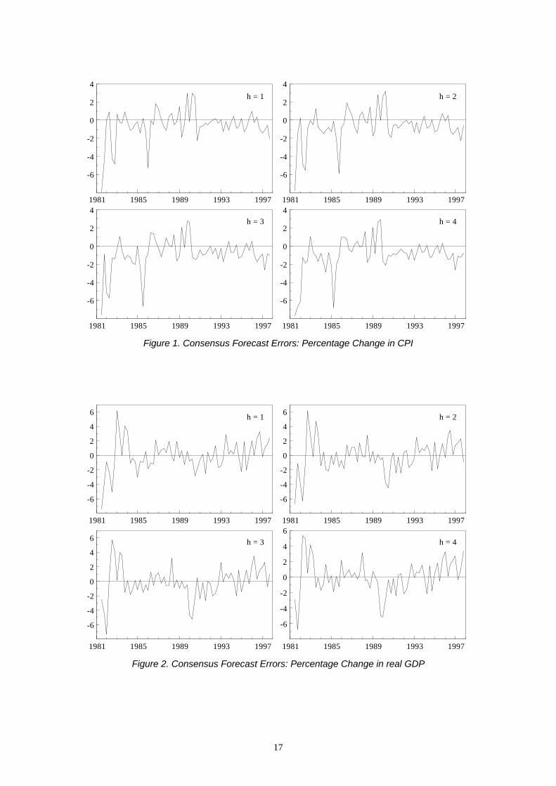
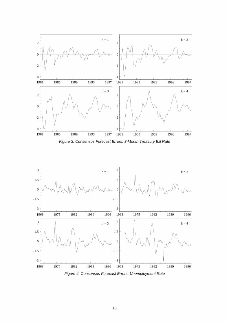
close to zero, while the mean GDP growth forecast errors are more varied. Figures 1-4

provide plots of the consensus forecast errors for each variable and horizon through time

(note that there are five quarters in which no survey respondents returned predictions for the

unemployment rate four steps ahead, thus the time series is broken in two places early on).

These plots show clearly the underprediction of inflation and the interest rate, and the relative

accuracy of the unemployment rate consensus forecasts. Excepting the GDP growth

forecasts, the pattern of standard deviations rising with the forecast horizon is again a feature

of the errors (see Table 2); this increase in volatility can be seen in the plots, particularly for

the T-bill rate and unemployment rate. The figures also highlight greater volatility exhibited

in the early 1980s for most of the series.

The distributions of consensus forecast errors appear to lack symmetry across the

variables and horizons, with negative skewness present in the case of inflation, GDP growth

and the interest rate, but postive skewness in the case of the unemployment rate.

Leptokurtosis is manifest in the consensus errors as well as individual forecasters’ errors,

with kurtosis estimates ranging from 4-8 (again treating the three and four steps ahead T-bill

rate forecasts as exceptions). The probability values associated with the null that the kurtosis

is three indicate rejection at very low significance levels, and the corresponding Student’s t

degrees of freedom are in the range 5-9, providing strong evidence that the consensus errors

8

are non-normal.

In contrast to the individual forecasts, the consensus series are not subject to the

problem of missing observations since there are always some survey returns in each period

for the variables and horizons we consider. The unbroken nature of these series therefore

admits the possibility of serial dependence analysis, overcoming to some extent the

aforementioned limitation of the individual series. However, there is one exception in our

data: the four steps ahead consensus forecasts of the unemployment rate have five missing

observations (as mentioned above). When examining serial dependence among these errors,

we use the longest unbroken segment of the series, which amounts to dropping the first

twenty four observations.

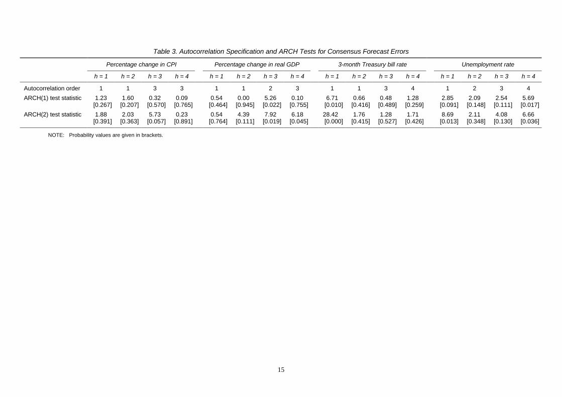
We examine two serial dependence properties of interest – the extent to which the

consensus forecast errors are autocorrelated, and whether the errors exhibit ARCH-type

behaviour. The order of autocorrelation present in a given consensus error time series is

found by fitting moving average models of varying order; the preferred model being chosen

by use of the Schwarz-Bayesian information criterion. Theoretically, optimal forecasts h-

steps ahead have dependence of order )1( −h , but since our consensus forecasts may well

lack optimality properties, higher order autocorrelation might be expected. Consequently, we

consider moving average orders )1( −h , h and )1( +h in our analysis. Table 3 contains the

autocorrelation orders resulting from this selection process. Autocorrelation of order one is

found to be present in all the one step ahead consensus forecasts; for longer horizons, the

orders vary between h and )1( −h .

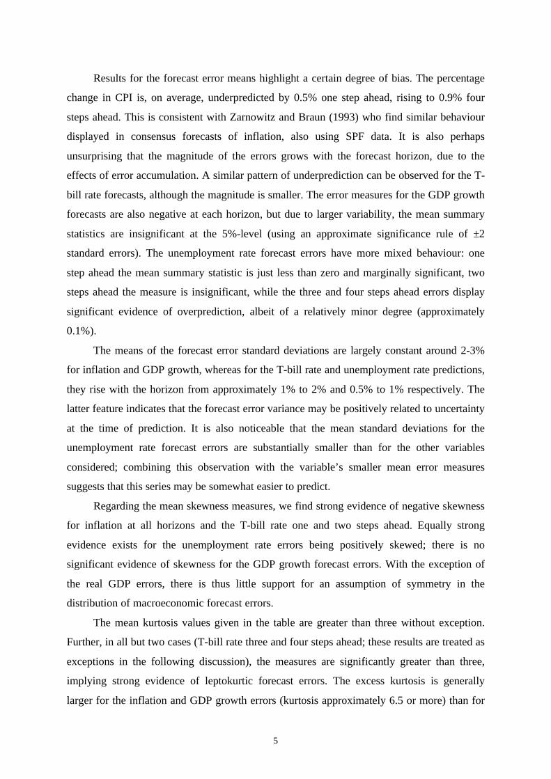
Testing for ARCH in the consensus forecast errors is performed using the standard

Engle (1982) test, although we first filter the errors for the autocorrelation found to be present

in the preceding analysis. The test is thus based on 2.RT in the regression

tptptt uuu ηααα ++++= −−22

1102 ˆ...ˆˆ

where 2ˆtu are the squared residuals from the preferred moving average model fitted to the

consensus forecast errors. The test statistic has an asymptotic 2χ distribution with p degrees

of freedom. Results of tests for relatively low order ARCH )2,1( =p are given in Table 3.

There is some evidence of ARCH in the consensus forecast errors we consider, but no

general patterns emerge. Variables and horizons for which there are rejections at

conventional significance levels in favour of ARCH error processes are inflation three steps

ahead, GDP growth three and four steps ahead, the T-bill rate one step ahead and the

9

unemployment rate one and four steps ahead. The somewhat anomalous ARCH(2) test

statistic for the one step ahead T-bill rate is driven by the first few observations: repetition of

the test with these observations omitted leads to a much reduced test statistic and non-

rejection of the null. The ARCH(1) test for this series is equally dependent on the first few

observations, casting doubt on an inference of ARCH in these consensus errors. Overall,

ARCH does seem to be present in some consensus errors at some horizons; however, the

sporadic nature of the evidence precludes any general inference across variables or horizons.

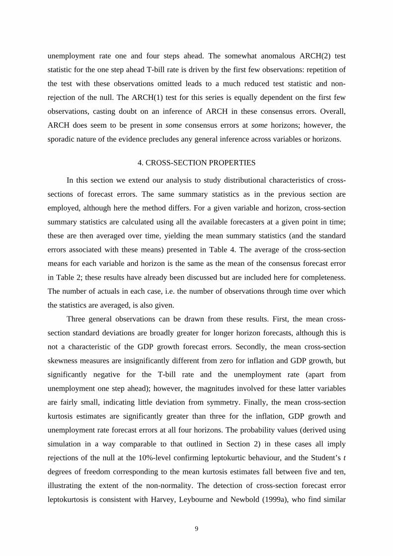
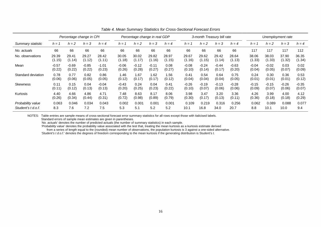
4. CROSS-SECTION PROPERTIES

In this section we extend our analysis to study distributional characteristics of cross-

sections of forecast errors. The same summary statistics as in the previous section are

employed, although here the method differs. For a given variable and horizon, cross-section

summary statistics are calculated using all the available forecasters at a given point in time;

these are then averaged over time, yielding the mean summary statistics (and the standard

errors associated with these means) presented in Table 4. The average of the cross-section

means for each variable and horizon is the same as the mean of the consensus forecast error

in Table 2; these results have already been discussed but are included here for completeness.

The number of actuals in each case, i.e. the number of observations through time over which

the statistics are averaged, is also given.

Three general observations can be drawn from these results. First, the mean cross-

section standard deviations are broadly greater for longer horizon forecasts, although this is

not a characteristic of the GDP growth forecast errors. Secondly, the mean cross-section

skewness measures are insignificantly different from zero for inflation and GDP growth, but

significantly negative for the T-bill rate and the unemployment rate (apart from

unemployment one step ahead); however, the magnitudes involved for these latter variables

are fairly small, indicating little deviation from symmetry. Finally, the mean cross-section

kurtosis estimates are significantly greater than three for the inflation, GDP growth and

unemployment rate forecast errors at all four horizons. The probability values (derived using

simulation in a way comparable to that outlined in Section 2) in these cases all imply

rejections of the null at the 10%-level confirming leptokurtic behaviour, and the Student’s t

degrees of freedom corresponding to the mean kurtosis estimates fall between five and ten,

illustrating the extent of the non-normality. The detection of cross-section forecast error

leptokurtosis is consistent with Harvey, Leybourne and Newbold (1999a), who find similar

10

properties among UK survey data on fixed event macroeconomic forecasts.

5. CONCLUSION

It is important for interval prediction and forecast evaluation to understand the

properties of forecast errors. This paper has investigated distributional and serial dependence

properties of errors from predictions of macroeconomic variables using a panel of US

forecasters. Analysis of summary measures of error for individual forecasters and the

consensus forecasts showed leptokurtosis to be a feature for almost all the variables and

horizons we considered. This result necessitates the conclusion that the frequently made

assumption of forecast error normality is untenable, its use resulting in overly narrow

prediction intervals and problems with evaluation tests reliant on such a premise. Further,

evidence of skewness was also displayed for a majority of variables and horizons in our

sample, strengthening the argument against forecast error normality.

Our recommendation is therefore to make use of robust or non-parametric forecast

evaluation tests, and in interval prediction, when an explicit distributional assumption is

required, to utilise the Student’s t distribution with relatively low degrees of freedom. On the

latter point, the t distribution is symmetric and does not permit skewness; if the possibility of

skewed forecast errors is also to be admitted, a more general distribution such as the non-

central t distribution (see, for example, Johnson and Kotz, 1970, chapter 31) may be

appropriate (as used by Lahiri and Teigland, 1987, in their analysis of SPF density forecasts).

In addition to these concerns, we found many of the forecast error series to have non-

zero mean, with underprediction being a feature of the inflation and interest rate forecasts.

ARCH was detected in some of the consensus forecast error time series, but not in general.

Finally, analysis of cross-sections of forecast errors highlighted a significant degree of cross-

section leptokurtosis.

11

REFERENCES

Baghestani, H. M. and Kianian, A. M. (1993), “On the Rationality of US Macroeconomic

Forecasts: Evidence from a Panel of Professional Forecasters”, Applied Economics, 25,

869-878.

Chatfield, C. (1993), “Calculating Interval Forecasts”, Journal of Business and Economic

Statistics, 11, 121-35.

Croushore, D. (1993), “The Survey of Professional Forecasters”, Business Review, Federal

Reserve Bank of Philadelphia, November/December, 3-15.

Diebold, F. X. and Mariano, R. S. (1995), “Comparing Predictive Accuracy”, Journal of

Business and Economic Statistics, 13, 253-263.

Diebold, F. X., Tay, A. S. and Wallis, K. F. (1999), “Evaluating Density Forecasts of

Inflation: The Survey of Professional Forecasters”, in Cointegration, Causality, and

Forecasting: A Festschrift in Honour of Clive W. J. Granger, eds. R. F. Engle and H.

White, New York: Oxford University Press.

Engle, R. F. (1982), “Autoregressive Conditional Heteroskedasticity with Estimates of the

Variance of United Kingdom Inflation”, Econometrica, 50, 987-1007.

Fair, R. C. and Shiller, R. J. (1989), “The Informational Content of Ex Ante Forecasts”,

Review of Economics and Statistics, 71, 325-331.

Harvey, D. I., Leybourne, S. J. and Newbold, P. (1997), “Testing the Equality of Prediction

Mean Squared Errors”, International Journal of Forecasting, 13, 281-291.

Harvey, D. I., Leybourne, S. J. and Newbold, P. (1998), “Tests for Forecast Encompassing”,

Journal of Business and Economic Statistics, 16, 254-259.

Harvey, D. I., Leybourne, S. J. and Newbold, P. (1999a), “Analysis of a Panel of UK

Macroeconomic Forecasts”, Loughborough Univeristy Economic Research Paper, No.

99/8.

Harvey, D. I., Leybourne, S. J. and Newbold, P. (1999b), “Forecast Evaluation Tests in the

Presence of ARCH”, Journal of Forecasting, 18, 435-445.

Johnson, N. L. and Kotz, S. (1970), Distributions in Statistics: Continuous Univariate

Distributions, Volume 2, Boston: Houghton Mifflin.

Keane, M. P. and Runkle, D. E. (1990), “Testing the Rationality of Price Forecasts: New

Evidence from Panel Data”, American Economic Review, 80, 714-735.

Kendall, M. G., Stuart, A. and Ord, J. K. (1987), Kendall’s Advanced Theory of Statistics,

Volume 1: Distribution Theory (5th ed.), London: Griffin.

Lahiri, K. and Teigland, C. (1987), “On the Normality of Probability Distributions of

Inflation and GNP Forecasts”, International Journal of Forecasting, 3, 269-279.

12

Tay, A. S. and Wallis, K. F. (2000), “Density Forecasting: A Survey”, Journal of

Forecasting, forthcoming.

Wallis, K. F. (1999), “Asymmetric Density Forecasts of Inflation and the Bank of England’s

Fan Chart”, National Institute Economic Review, 167, 106-112.

Zarnowitz, V. (1969), “The New ASA--NBER Survey of Forecasts by Economic

Statisticians”, American Statistician, 23, 12-16.

Zarnowitz, V. (1984), “The Accuracy of Individual and Group Forecasts from Business

Outlook Surveys”, Journal of Forecasting, 3, 11-26.

Zarnowitz, V. (1985), “Rational Expectations and Macroeconomic Forecasts”, Journal of

Business and Economic Statistics, 3, 293-311.

Zarnowitz, V. and Braun, P. (1993), “Twenty-Two Years of the NBER-ASA Quarterly

Economic Outlook Surveys: Aspects and Comparisons of Forecasting Performance”, in

Business Cycles, Indicators, and Forecasting, eds. J. H. Stock and M. W. Watson,

Chicago: University of Chicago Press.

Zarnowitz, V. and Lambros, L. A. (1987), “Consensus and Uncertainty in Economic

Prediction”, Journal of Political Economy, 95, 591-621.

13

Table 1. Mean Summary Statistics for Individual Forecaster Errors

Percentage change in CPI Percentage change in real GDP 3-month Treasury bill rate Unemployment rate

Summary statistic h = 1 h = 2 h = 3 h = 4 h = 1 h = 2 h = 3 h = 4 h = 1 h = 2 h = 3 h = 4 h = 1 h = 2 h = 3 h = 4

No. forecasters 11 11 11 11 11 11 11 11 11 11 11 11 47 47 47 39

No. observations 45.36 45.45 45.36 43.55 47.45 47.36 47.27 45.36 46.91 46.82 46.55 44.91 45.53 45.51 45.38 44.38(2.20) (2.14) (2.08) (1.56) (1.74) (1.74) (1.68) (1.25) (1.99) (1.99) (1.92) (1.48) (2.02) (2.02) (2.00) (1.95)

Mean -0.51 -0.60 -0.78 -0.91 -0.31 -0.46 -0.27 -0.13 -0.13 -0.32 -0.48 -0.66 -0.03 0.03 0.12 0.11(0.08) (0.08) (0.11) (0.13) (0.17) (0.26) (0.18) (0.24) (0.07) (0.10) (0.12) (0.15) (0.01) (0.02) (0.03) (0.03)

Standard deviation 2.02 2.00 1.99 2.18 2.84 3.51 3.38 2.79 0.98 1.32 1.59 1.84 0.48 0.71 0.90 0.98(0.11) (0.11) (0.13) (0.12) (0.27) (0.38) (0.43) (0.15) (0.07) (0.07) (0.09) (0.10) (0.01) (0.02) (0.02) (0.02)

Skewness -0.98 -0.76 -0.75 -1.09 0.11 -0.62 -0.21 0.06 -0.85 -0.63 -0.19 -0.07 0.67 0.92 0.95 0.90(0.23) (0.24) (0.21) (0.27) (0.48) (0.72) (0.80) (0.42) (0.32) (0.26) (0.16) (0.16) (0.07) (0.06) (0.06) (0.08)

Kurtosis 6.68 6.51 5.49 6.95 7.30 11.82 12.28 6.84 6.19 4.80 3.20 3.03 4.31 4.82 4.61 4.32(0.54) (0.72) (0.46) (0.77) (2.28) (3.37) (4.23) (1.19) (1.04) (0.75) (0.22) (0.32) (0.17) (0.18) (0.16) (0.16)

Probability value 0.001 0.002 0.009 0.002 0.001 0.000 0.000 0.001 0.002 0.022 0.301 0.398 0.049 0.022 0.031 0.050Student’s t d.o.f. 5.6 5.7 6.4 5.5 5.4 4.7 4.6 5.6 5.9 7.3 34.0 204.0 8.6 7.3 7.7 8.5

NOTES: Table entries are sample means of individual forecaster error summary statistics for all rows except those with italicised labels.Standard errors of sample mean estimates are given in parentheses.‘No. forecasters’ denotes the number of forecasters (the number of summary statistics) in each sample.‘Probability value’ denotes the probability value associated with the test that, treating the mean kurtosis as a kurtosis estimate derived

from a series of length equal to the (rounded) mean number of observations, the population kurtosis is 3 against a one-sided alternative.‘Student’s t d.o.f.’ denotes the degrees of freedom corresponding to the mean kurtosis if the generating distribution is Student’s t.

14

Table 2. Summary Statistics for Consensus Forecast Errors

Percentage change in CPI Percentage change in real GDP 3-month Treasury bill rate Unemployment rate

Summary statistic h = 1 h = 2 h = 3 h = 4 h = 1 h = 2 h = 3 h = 4 h = 1 h = 2 h = 3 h = 4 h = 1 h = 2 h = 3 h = 4

No. observations 66 66 66 66 66 66 66 66 66 66 66 66 117 117 117 112

Mean -0.57 -0.69 -0.85 -1.01 -0.06 -0.12 -0.11 0.08 -0.08 -0.24 -0.44 -0.63 -0.04 -0.02 0.03 0.02

Standard deviation 1.76 1.77 1.78 1.86 2.11 2.24 2.21 2.17 0.83 1.13 1.37 1.60 0.39 0.59 0.78 0.96

Skewness -1.54 -1.39 -1.53 -1.53 -0.28 -0.30 -0.34 -0.33 -1.19 -0.77 -0.40 -0.23 0.79 1.09 1.16 0.70

Kurtosis 8.07 7.90 7.81 7.58 5.20 4.58 4.76 4.45 6.19 4.31 3.20 2.70 4.15 5.22 5.24 5.21

Probability value 0.000 0.000 0.000 0.000 0.005 0.016 0.011 0.023 0.001 0.030 0.296 0.669 0.018 0.001 0.001 0.001Student’s t d.o.f. 5.2 5.2 5.2 5.3 6.7 7.8 7.4 8.1 5.9 8.6 34.0 - 9.2 6.7 6.7 6.7

NOTES: Table entries are consensus forecast error summary statistics for all rows except those with italicised labels.‘Probability value’ denotes the probability value associated with the test that the population kurtosis is 3 against a one-sided alternative.‘Student’s t d.o.f.’ denotes the degrees of freedom corresponding to the kurtosis if the generating distribution is Student’s t.

15

Table 3. Autocorrelation Specification and ARCH Tests for Consensus Forecast Errors

Percentage change in CPI Percentage change in real GDP 3-month Treasury bill rate Unemployment rate

h = 1 h = 2 h = 3 h = 4 h = 1 h = 2 h = 3 h = 4 h = 1 h = 2 h = 3 h = 4 h = 1 h = 2 h = 3 h = 4

Autocorrelation order 1 1 3 3 1 1 2 3 1 1 3 4 1 2 3 4

ARCH(1) test statistic 1.23 1.60 0.32 0.09 0.54 0.00 5.26 0.10 6.71 0.66 0.48 1.28 2.85 2.09 2.54 5.69[0.267] [0.207] [0.570] [0.765] [0.464] [0.945] [0.022] [0.755] [0.010] [0.416] [0.489] [0.259] [0.091] [0.148] [0.111] [0.017]

ARCH(2) test statistic 1.88 2.03 5.73 0.23 0.54 4.39 7.92 6.18 28.42 1.76 1.28 1.71 8.69 2.11 4.08 6.66[0.391] [0.363] [0.057] [0.891] [0.764] [0.111] [0.019] [0.045] [0.000] [0.415] [0.527] [0.426] [0.013] [0.348] [0.130] [0.036]

NOTE: Probability values are given in brackets.

16

Table 4. Mean Summary Statistics for Cross-Sectional Forecast Errors

Percentage change in CPI Percentage change in real GDP 3-month Treasury bill rate Unemployment rate

Summary statistic h = 1 h = 2 h = 3 h = 4 h = 1 h = 2 h = 3 h = 4 h = 1 h = 2 h = 3 h = 4 h = 1 h = 2 h = 3 h = 4

No. actuals 66 66 66 66 66 66 66 66 66 66 66 66 117 117 117 112

No. observations 29.39 29.41 29.27 28.42 30.05 30.02 29.82 28.97 29.67 29.62 29.42 28.64 38.06 38.03 37.90 36.35(1.15) (1.14) (1.12) (1.11) (1.18) (1.17) (1.16) (1.15) (1.16) (1.15) (1.14) (1.13) (1.33) (1.33) (1.32) (1.34)

Mean -0.57 -0.69 -0.85 -1.01 -0.06 -0.12 -0.11 0.08 -0.08 -0.24 -0.44 -0.63 -0.04 -0.02 0.03 0.02(0.22) (0.22) (0.22) (0.23) (0.26) (0.28) (0.27) (0.27) (0.10) (0.14) (0.17) (0.20) (0.04) (0.05) (0.07) (0.09)

Standard deviation 0.78 0.77 0.82 0.86 1.46 1.67 1.62 1.56 0.41 0.54 0.64 0.75 0.24 0.30 0.36 0.53(0.06) (0.06) (0.05) (0.05) (0.12) (0.17) (0.17) (0.12) (0.04) (0.04) (0.04) (0.05) (0.01) (0.01) (0.01) (0.12)

Skewness 0.11 0.15 0.04 -0.04 -0.43 0.24 0.04 0.41 -0.26 -0.19 -0.13 -0.28 -0.15 -0.15 -0.26 -0.35(0.11) (0.12) (0.13) (0.13) (0.20) (0.25) (0.23) (0.22) (0.10) (0.07) (0.06) (0.06) (0.09) (0.07) (0.06) (0.07)

Kurtosis 4.40 4.66 4.86 4.71 7.48 8.63 8.17 8.06 3.98 3.47 3.20 3.36 4.26 3.99 4.00 4.12(0.26) (0.34) (0.44) (0.31) (0.72) (0.98) (0.89) (0.79) (0.30) (0.17) (0.13) (0.11) (0.36) (0.18) (0.18) (0.29)

Probability value 0.063 0.046 0.034 0.043 0.002 0.001 0.001 0.001 0.109 0.219 0.316 0.256 0.062 0.089 0.088 0.077Student’s t d.o.f. 8.3 7.6 7.2 7.5 5.3 5.1 5.2 5.2 10.1 16.8 34.0 20.7 8.8 10.1 10.0 9.4

NOTES: Table entries are sample means of cross-sectional forecast error summary statistics for all rows except those with italicised labels.Standard errors of sample mean estimates are given in parentheses.‘No. actuals’ denotes the number of predicted actuals (the number of summary statistics) in each sample.‘Probability value’ denotes the probability value associated with the test that, treating the mean kurtosis as a kurtosis estimate derived

from a series of length equal to the (rounded) mean number of observations, the population kurtosis is 3 against a one-sided alternative.‘Student’s t d.o.f.’ denotes the degrees of freedom corresponding to the mean kurtosis if the generating distribution is Student’s t.

17

1981 1985 1989 1993 1997

-6

-4

-2

0

2

4

h = 1

1981 1985 1989 1993 1997

-6

-4

-2

0

2

4

h = 2

1981 1985 1989 1993 1997

-6

-4

-2

0

2

4h = 3

1981 1985 1989 1993 1997

-6

-4

-2

0

2

4h = 4

Figure 1. Consensus Forecast Errors: Percentage Change in CPI

1981 1985 1989 1993 1997

-6

-4

-2

0

2

4

6h = 1

1981 1985 1989 1993 1997

-6

-4

-2

0

2

4

6h = 2

1981 1985 1989 1993 1997

-6

-4

-2

0

2

4

6 h = 3

1981 1985 1989 1993 1997

-6

-4

-2

0

2

4

6h = 4

Figure 2. Consensus Forecast Errors: Percentage Change in real GDP

18

1981 1985 1989 1993 1997

-4

-2

0

2h = 1

1981 1985 1989 1993 1997

-4

-2

0

2h = 2

1981 1985 1989 1993 1997

-4

-2

0

2h = 3

1981 1985 1989 1993 1997

-4

-2

0

2h = 4

Figure 3. Consensus Forecast Errors: 3-Month Treasury Bill Rate

1968 1975 1982 1989 1996

-3

-1.5

0

1.5

3 h = 1

1968 1975 1982 1989 1996

-3

-1.5

0

1.5

3 h = 2

1968 1975 1982 1989 1996

-3

-1.5

0

1.5

3 h = 3

1968 1975 1982 1989 1996

-3

-1.5

0

1.5

3 h = 4

Figure 4. Consensus Forecast Errors: Unemployment Rate