11

Proper Univariate and Proper Univariate and Multivariate IntegralsMultivariate Integrals

Rajandra Chadra BhowmikRajandra Chadra BhowmikLecturerLecturer

Dept. of MathematicsDept. of MathematicsPabna Science and Technology UniversityPabna Science and Technology University

( )b

a

f x dx

2

• What is the volume of a sphere?

-1-0.5

00.5

1 0

0.5

10

0.5

1

1.5

2

2.5

3

3.5

y-axis

x = cos(t), y = sin(t), z = t in 0 <= t <= pi

x-axis

z-ax

is • What is the mass of a wire?

if density is given???

How is it = 4*pi*radius3/3

???

-6 -4 -2 0 2 4 6

-5

-4

-3

-2

-1

0

1

2

3

4

5

x-axis

y-ax

is

Area of the circle x.2+y.2=25

y=sqrt(25-x2)

x = 0 y = 0

R1

x = 5

• What is the area of a circle?

How is it = pi*(radius)2

???

Let’s start with some classical problems

3

Lecture contents

1.1. Pre-history and ArchimedesPre-history and Archimedes2.2. Invention of Newton and Leibnitz Invention of Newton and Leibnitz 3.3. Definite integrals and RiemannDefinite integrals and Riemann4.4. Geometric Interpretation and Applications Geometric Interpretation and Applications

of Definite Integralsof Definite Integrals5.5. Double Integrals and Triple IntegralsDouble Integrals and Triple Integrals6.6. Applications of Double Integrals and Triple Applications of Double Integrals and Triple

IntegralsIntegrals7.7. Line IntegralsLine Integrals8.8. Applications of Line IntegralsApplications of Line Integrals

4

Pre-history and ArchimedesPre-history and Archimedes

• Integration can be traced as far back as

ancient Egypt, circa 1800 BC, with the

Moscow Mathematical Papyrus

demonstrating knowledge of a formula for

the volume of a pyramidal frustum.

• The first documented systematic technique

capable of determining integrals is the

method of exhaustion of Eudoxus (circa 370

BC), which sought to find areas and

volumes by breaking them up into an infinite

number of shapes for which the area or

volume was known.

• This method was further developed and

employed by Archimedes (287 BC - 212

BC) and used to calculate areas for

parabolas and an approximation to the area

of a circle.

Archimedes devised a heuristic method based on statistics to do private calculations that would be classified today as integral calculus, but then presented rigorous geometric proofs for his results. To what extent Archimedes’ version of integral calculus was correct is debatable.

5

Invention of Newton and LeibnitzInvention of Newton and Leibnitz• The major advance in integration came in the 17th

century with the independent discovery of the fundamental theorem of calculus by Newton (1642-1727) and Leibnitz (1646-1716).

• The theorem demonstrates a connection between integration and differentiation. This connection, combined with the comparative ease of differentiation, can be exploited to calculate integrals.

• In particular, the fundamental theorem of calculus allows one to solve a much broader class of problems. Equal in importance is the comprehensive mathematical framework that both Newton and Leibnitz developed. Given the name infinitesimal calculus, it allowed for precise analysis of functions within continuous domains. This framework eventually became modern calculus, whose notation for integrals is drawn directly from the work of Leibnitz.

6

• While Newton and Leibnitz provided a systematic approach to integration, their work lacked a degree of rigor.

• Bishop Berkeley memorably attacked infinitesimals as "the ghosts of departed quantities".

• Calculus acquired a firmer footing with the development of limits and was given a suitable foundation by Cauchy in the first half of the 19th century.

Drawbacks of Newton and LeibnitzDrawbacks of Newton and Leibnitz

7

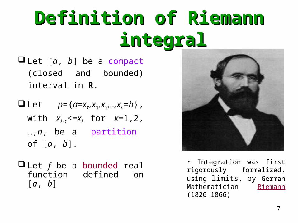
Definition of Riemann integralDefinition of Riemann integral

Let [a, b] be a compact

(closed and bounded)

interval in R.

Let p={a=x0,x1,x2,..,xn=b},

with xk-1<=xk for k=1,2,

…,n, be a partition of [a,

b].

Let f be a bounded real function defined on [a, b]

• Integration was first rigorously formalized, using limits, by German Mathematician Riemann (1826-1866)

8

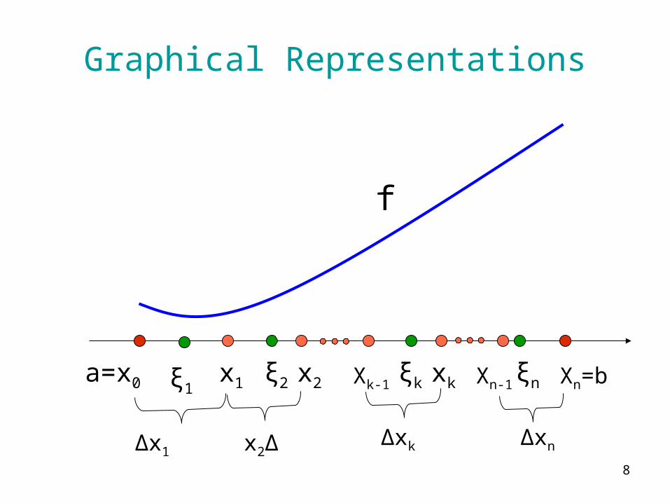
Graphical Representations

a=x0 ξ1x1 Xk-1

xk Xn-1

∆x1∆xk∆x2

Xn=b

∆xn

ξ2 x2 ξnξk

f

9

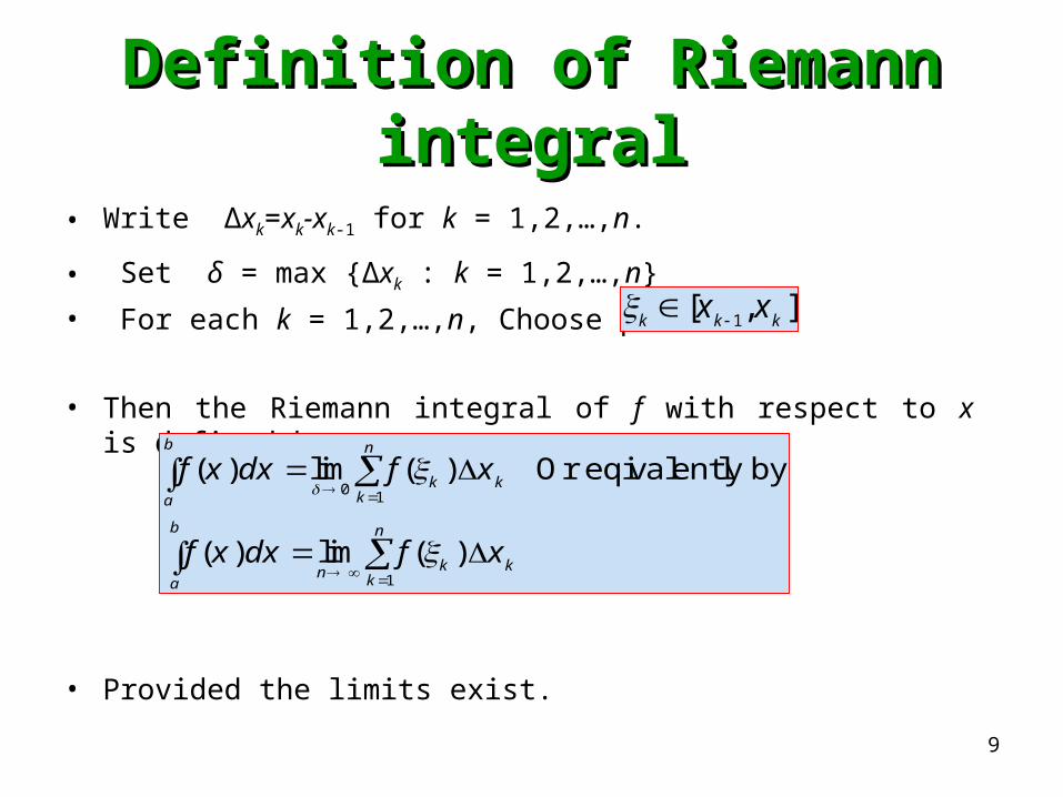
Definition of Riemann integralDefinition of Riemann integral

• Write ∆xk=xk-xk-1 for k = 1,2,…,n.

• Set δ = max {∆xk : k = 1,2,…,n}

• For each k = 1,2,…,n, Choose point

• Then the Riemann integral of f with respect to x is defined by

• Provided the limits exist.

0 1

1

( ) lim ( ) Or eqivalently by

( ) lim ( )

b n

k kka

b n

k kn ka

f x dx f x

f x dx f x

1 [ , ]k k kx x

10

Graphical Representations

x0=a ξ1x1 Xk-1

xk Xn-1

∆x1∆xk∆x2

Xn=b

∆xn

ξ2 x2 ξnξk

f(ξ1)f(ξ2)

f(ξk)

f(ξn)

f

f(ξ1)∆x1

f(ξ2)∆x2

f(ξk)∆xk

f(ξn)∆xn

11

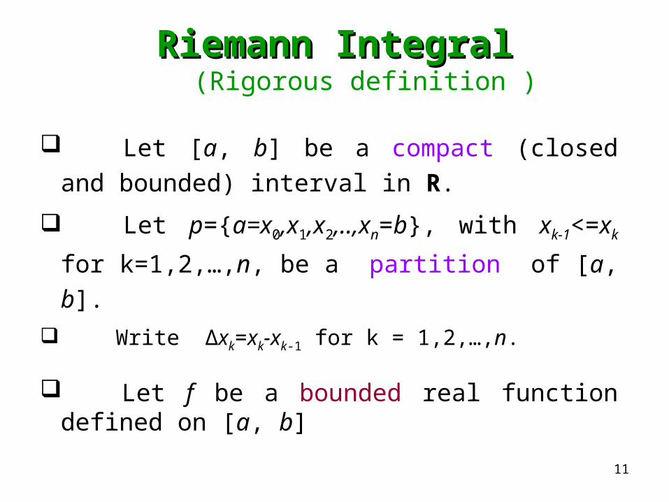
Riemann IntegralRiemann Integral(Rigorous definition )

Let [a, b] be a compact (closed and

bounded) interval in R.

Let p={a=x0,x1,x2,..,xn=b}, with xk-1<=xk

for k=1,2,…,n, be a partition of [a, b].

Write ∆xk=xk-xk-1 for k = 1,2,…,n.

Let f be a bounded real function defined on [a, b]

12

Corresponding to each partition P, and k=1,2,…n, put

And then

1

1

( , )

( , )

n

k kk

n

k kk

U P f M x

L P f m x

1

1

sup{ ( ) : }

inf { ( ) : }k k k

k k k

M f x x x x

m f x x x x

13

Lower sum L(P, f)

x0=a x1 x2 x3Xk-1 xk Xn-1

∆x1∆xk∆x3∆x2

Xn=b

∆xn

m1 ∆x1m3 ∆x3

m2 ∆x2

mk ∆xk

mn ∆xn

f

14

Upper sum U(P, f)

x0=a x1 x2 x3Xk-1 xk Xn-1

∆x1∆xk∆x3∆x2

Xn=b

∆xn

M1 ∆x1M3 ∆x3

M2 ∆x2Mk ∆xk

Mn ∆xn

f

15

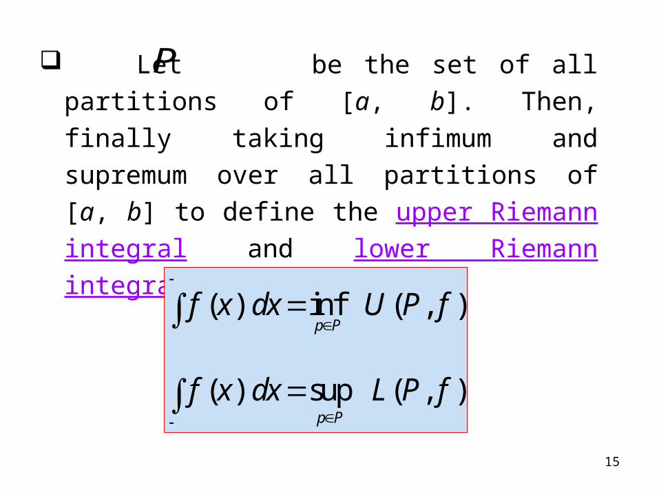
Let be the set of all partitions of [a, b].

Then, finally taking infimum and supremum

over all partitions of [a, b] to define the upper

Riemann integral and lower Riemann integral

respectively as

( ) inf ( , )

( ) sup ( , )

p

p

f x dx U P f

f x dx L P f

P

P

P

16

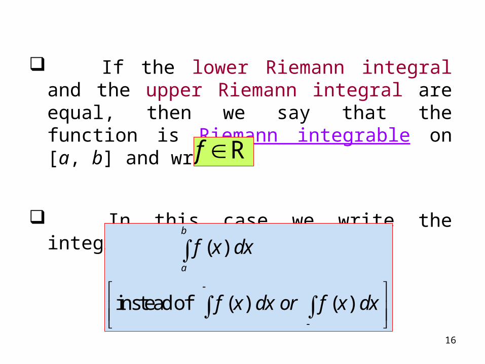
If the lower Riemann integral and the upper Riemann integral are equal, then we say that the function is Riemann integrable on [a, b] and write

In this case we write the integral as

( )

insteadof ( ) ( )

b

a

f x dx

f x dx or f x dx

f R

17

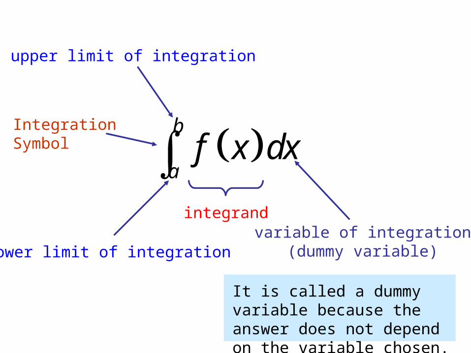
b

af x dx

IntegrationSymbol

lower limit of integration

upper limit of integration

integrandvariable of integration

(dummy variable)

It is called a dummy variable because the answer does not depend on the variable chosen.

18

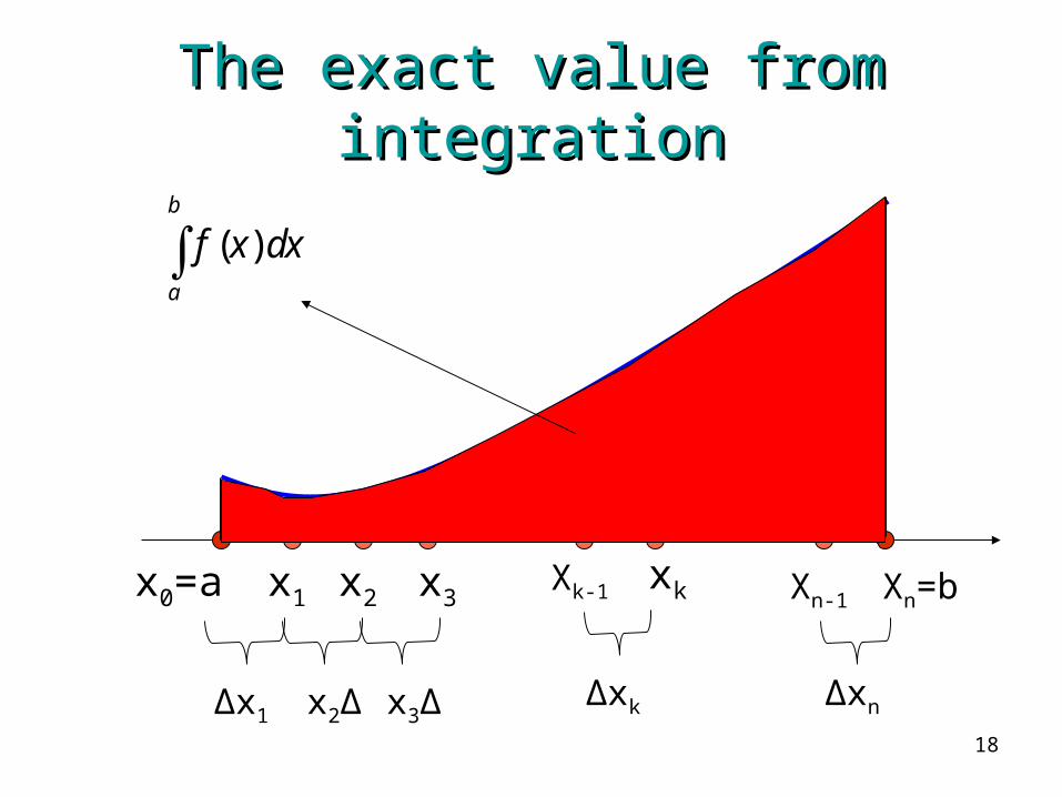
The exact value from The exact value from integrationintegration

x0=a x1 x2 x3Xk-1 xk Xn-1

∆x1∆xk∆x3∆x2

Xn=b

∆xn

( )b

a

f x dx

19

Some results

For every P,

For any refinement P*(a super set of P) of P,

( ) ( )f x dx f x dx

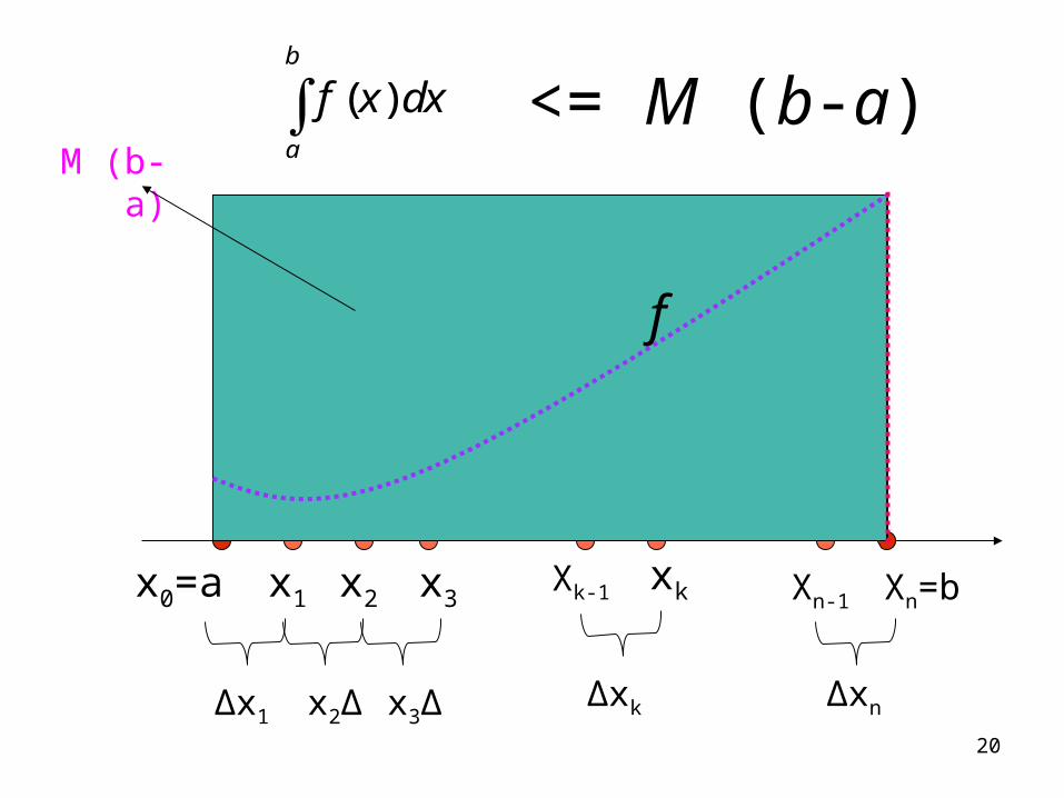
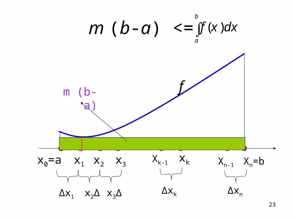
( ) ( , ) ( , ) ( )m b a L P f U P f M b a

( , ) ( *, ) ( *, ) ( , )L P f L P f U P f U P f

20

<= M (b-a)

x0=a x1 x2 x3Xk-1 xk Xn-1

∆x1∆xk∆x3∆x2

Xn=b

∆xn

M (b-a)

( )b

a

f x dx

f

21

<= U (P1, f) <= M (b-a)

x0=a X1

∆x1

X2=b

∆x2

M1 ∆x1

M2 ∆x2

( )b

a

f x dx

f

22

<=U (P2, f)<= U (P1, f) <= M (b-a)

x0=a X1

∆x1

X2=b

∆x2

M1 ∆x1

M2 ∆x2

∆x3

M3 ∆x3

X2

f

( )b

a

f x dx

23

m (b-a) <=

x0=a x1 x2 x3Xk-1 xk Xn-1

∆x1∆xk∆x3∆x2

Xn=b

∆xn

m (b-a) f

( )b

a

f x dx

24

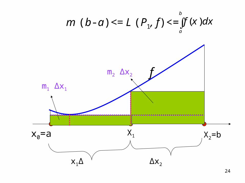
m (b-a)<= L (P1, f)<=

x0=a X1

∆x1

X2=b

∆x2

m1 ∆x1

m2 ∆x2 f

( )b

a

f x dx

25

m (b-a) <= L (P1, f) <= L (P2, f) <=

x0=a X1

∆x1

X2=b

∆x2

m1 ∆x1m2 ∆x2

∆x3

m3 ∆x3

( )b

a

f x dx

X2

f

26

Necessary and sufficient Necessary and sufficient conditionsconditions

f is continuous on [a, b] implies f is Riemann integrable on [a, b].

f is monotonic on [a, b] implies f is Riemann integrable on [a, b].

f is bounded on [a, b] and f has only finitely many points of discontinuity on [a, b] implies f is Riemann integrable on [a, b].

A bounded function f on a compact interval is integrable iff its set of discontinuities has measure zero(0).

Proof of the Theorem is out of scope here (a matter of Lebesgue Integration in Measure Theory). For instant, we only say that all countable sets, including finite sets, and the Cantor set have measure 0, so that functions that are discontinuous only on these sets are integrable.

0

Riemann integrable

,

( , ) - ( , )

A function f is if

for every there exist a partition P

such that U P f L P f

27

Dirichlet function and Thomae function

1( )

0

when xd x

when x

Q

Q

1 0

1( ) , 0, ,gcd( , ) 1

0

when x

pt x when x q p p q

q q

when x

Z

Q

Both functions are bounded.

First one is discontinuous

everywhere in R. i.e. the set of

discontinuities has a nonzero

measure. On the other hand,

second one is discontinuous

only at the rationals. i.e. set

of discontinuities has measure 0.

So, Dirichlet function is not integrable but Thomae function is.

28

Properties of Riemann Properties of Riemann integralintegral

RR R

R

R

R

, [ , ] .

) ( )

)

) ( ) ( ) [ , ]

) .

b b b

a a a

b b

a a

b b

a a

Let f g on a b and Then

i f g and f g dx f dx g dx

ii f and f dx f dx

iii f x g x in a b f dx g dx

iv fg

0 0

R [ , ].

)

)

) , ( , )

b

a

b a

a b

b c b

a a c

Let f on a b Then

i f f dx

ii f dx f dx

iii f dx f dx f dx for some c a b

Let R on Then

on

R

[ , ].

) ( ) [ , ] ( )

)

b

a

b b

a a

f a b

i f x M a b f dx M b a

ii f and f dx f dx

29

Fundamental Theorem of Calculus (Part 1)Fundamental Theorem of Calculus (Part 1)

/

Riemann integrable

[ , ].

[ , ] ,

( ) ( ) ( ). b

a

Let f be a real function

on a b And if there be a differentiable

function F on a b such that F f then

f x dx F b F a

30

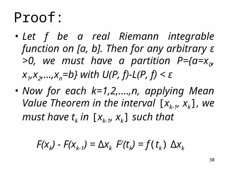
Proof: • Let f be a real Riemann integrable function

on [a, b]. Then for any arbitrary ε >0, we must have a partition P={a=x0, x1,x2,…,xn=b} with U(P, f)-L(P, f) < ε

• Now for each k=1,2,….,n, applying Mean Value Theorem in the interval [xk-1, xk], we must have tk in [xk-1, xk] such that

F(xk) - F(xk-1) = ∆xk F/(tk) = f(tk) ∆xk

31

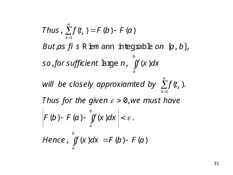
1

1

0

, ( ) ( ) ( )

, Riemann integrable [ , ],

, large , ( )

( ).

,

( ) ( ) ( ) .

, ( ) (

n

kk

b

a

n

kk

b

a

b

a

Thus f t F b F a

But as f is on a b

so for sufficient n f x dx

will be closely approxiamted by f t

Thus for the given we must have

F b F a f x dx

Hence f x dx F ) ( )b F a

32

Fundamental Theorem of Calculus (Part 2)Fundamental Theorem of Calculus (Part 2)

Riemann integrable [ , ].

, ( ) ( ) .

[ , ]; ,

int [ , ],

,

x

a

Let f be a real fuction on a b

For a x b put F x f t dt

Then F is continuous on a b furthermore

if f is continuous at a po c of a b

then F is differentiable at c a

/

( ) ( )

nd

F c f c

33

Proof:

[ , ], ,

( ) [ , ].

, [ , ] ,

( ) ( ) ( ) ( )

( ) ( )......(*)

y x

a a

y

x

Since f on a b so f is bounded and thus

say f x M for all x a b

Now for any x y a b with x y

F y F x f x dx f x dx

f x dx M y x

R

34

Continue:

0 ( ) ( )

, (*), / , [ , ]

( ) ( ) .

( )

Let begivensatisfying F y F x

Then for M and for all x y a b

y x F y F x

whichshows theuniformcontinuity of F

using

35

Continue:

0 0

suppose [ , ].

,

( ) ( ) [ , ]....(**)

using(**) , [ , ]

,

( )( ) ( )( )

Now that f is continuous at c a b

Thus for any given weget suchthat

f x f c whenever x c for all x a b

Now for some s t a b with s c t satisfying

x c wehave

f x dxF t F sf c

t s

1

/

( ) ( )( )

( ) ( )

( ) ( )

t t t

s s s

t

s

f x dx f c dxf c

t s t s t s

f x f c dxt s

This follows that F c f c

36

Drawbacks of Riemann Drawbacks of Riemann IntegralIntegral

• Although all bounded piecewise continuous functions are Riemann integrable on a bounded interval, subsequently more general functions were considered, to which Riemann's definition does not apply.

• Stieltje formulated an integral called Stietjes integral, to which Riemann integral is a special case.

• Lebesgue formulated a different definition of integral, founded in measure theory (a subfield of real analysis).

• Other definitions of integral, extending Riemann's and Lebesgue's approaches, were proposed.

37

Drawbacks of Riemann Drawbacks of Riemann IntegralIntegral

A major limitation towards more widespread implementation of Bayesian approaches is that obtaining the posterior distribution often requires the integration of high-dimensional functions. This can be computationally very difficult, among the several approaches short of direct integration Markov Chain Monte Carlo (MCMC) methods is one which attempt to simulate direct draws from some complex distribution of interest.

MCMC approaches are so-named because one uses the previous sample values to randomly generate the next sample value, generating a Markov chain (as the transition probabilities between sample values are only a function of the most recent sample value).

38

Drawbacks of Riemann Drawbacks of Riemann IntegralIntegral

Markov chain Monte Carlo integration, or MCMC, is a term used to cover a broad range of methods for numerically computing probabilities, or for optimization. They are simulation methods, mostly used in complex stochastic systems where exact computation and even simple simulation are not computationally feasible.

Methods that fall under this heading include Metropolis sampling, Hastings sampling and Gibbs sampling which are for integration and simulated annealing and sometimes genetic algorithms which are optimization techniques.

Although these methods are mainly used for complex systems it can be used to find the exact p-value for a test of association between the rows and columns of a contingency table.

39

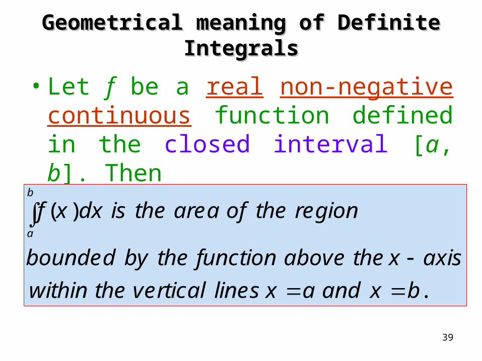
Geometrical meaning of Definite IntegralsGeometrical meaning of Definite Integrals

• Let f be a real non-negative continuous function defined in the closed interval [a, b]. Then

( )

.

b

a

f x dx is the area of the region

bounded by the function above the x axis

within the vertical lines x a and x b

40

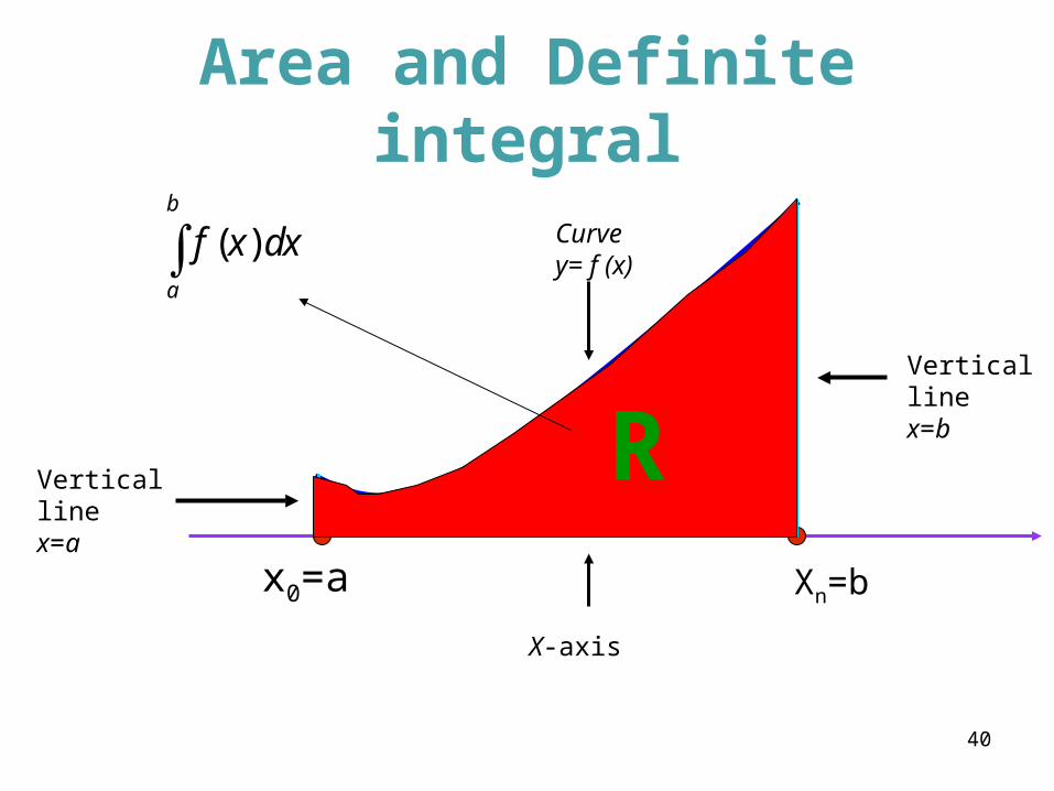
Area and Definite integral

x0=a Xn=b

( )b

a

f x dx

RVertical linex=b

Vertical linex=a

X-axis

Curve y= f (x)

41

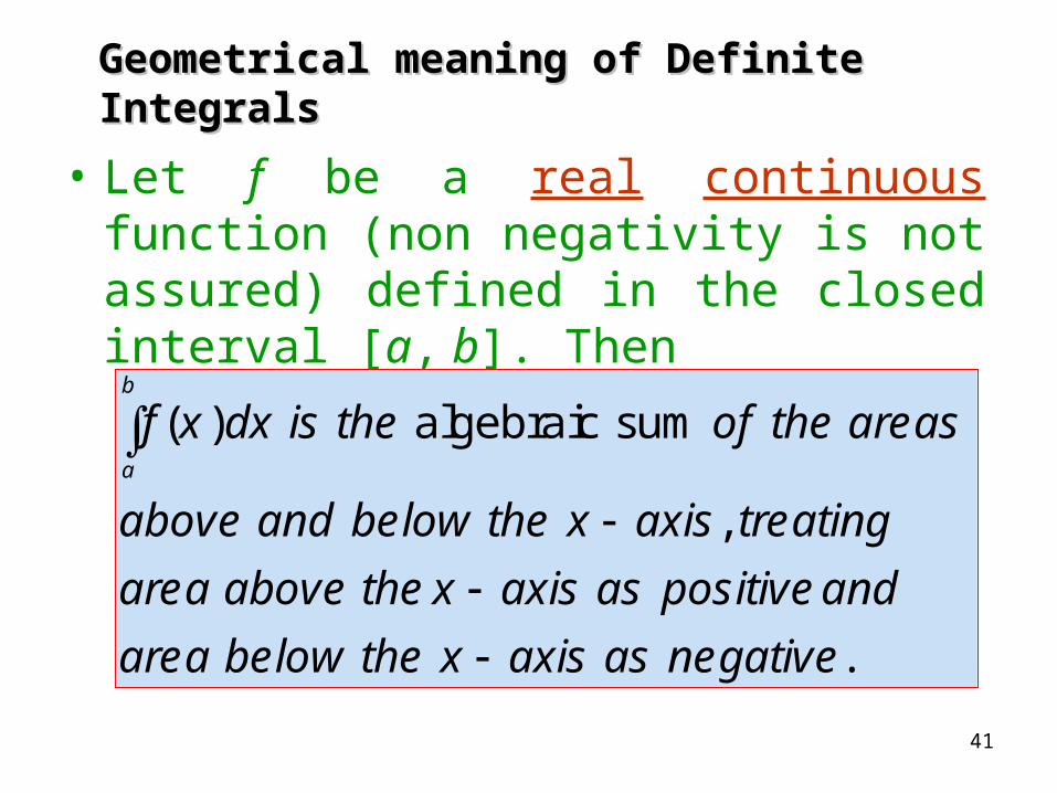
• Let f be a real continuous function (non negativity is not assured) defined in the closed interval [a, b]. Then

( ) algebraic sum

,

.

b

a

f x dx is the of the areas

above and below the x axis treating

area above the x axis as positiveand

area below the x axis as negative

Geometrical meaning of Definite IntegralsGeometrical meaning of Definite Integrals

42

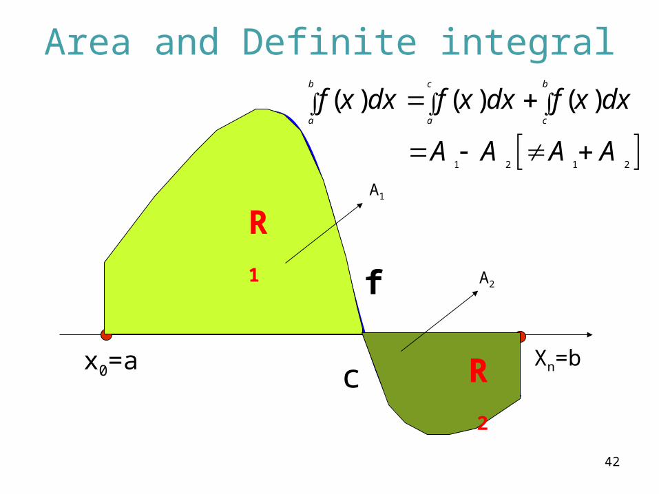
Area and Definite integral

x0=a Xn=b

R 1

R 2

f

c

1 2 1 2

( ) ( ) ( )b c b

a a c

f x dx f x dx f x dx

A A A A

A1

A2

43

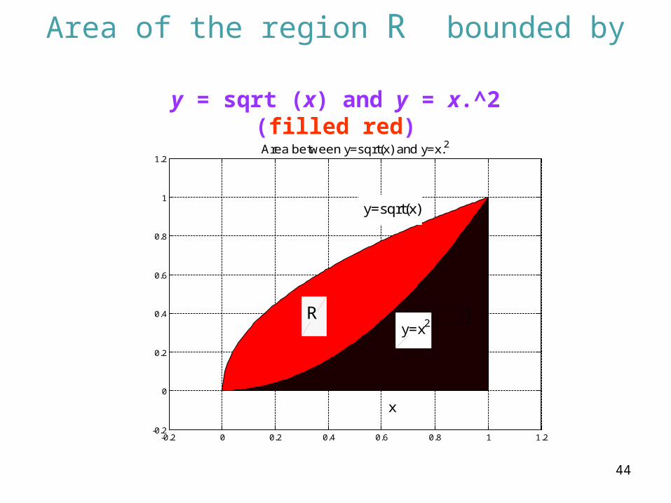
Applications of Definite Integrals (1)Applications of Definite Integrals (1) (Area of a region) (Area of a region)

Let f and g are continuous functions on the interval [a, b] with

f (x) >= g (x) in [a, b]. Then the area A of the region

• bounded above by the curve y = f (x)

• below by the curve y = g (x)

• between the vertical line x =a and x = b is given by

( ) ( )b

x a

A f x g x dx

44

Area of the region R bounded by y = sqrt (x) and y = x.^2

(filled red)

-0.2 0 0.2 0.4 0.6 0.8 1 1.2-0.2

0

0.2

0.4

0.6

0.8

1

1.2Area between y=sqrt(x) and y=x.2

y=x.2

y=sqrt(x)

y=x2

x

R

45

12

0

A x x dx

-0.2 0 0.2 0.4 0.6 0.8 1 1.2-0.2

0

0.2

0.4

0.6

0.8

1

Area between y=sqrt(x) and y=x.2

y=x.2

y=sqrt(x)

y=x2R

x

46

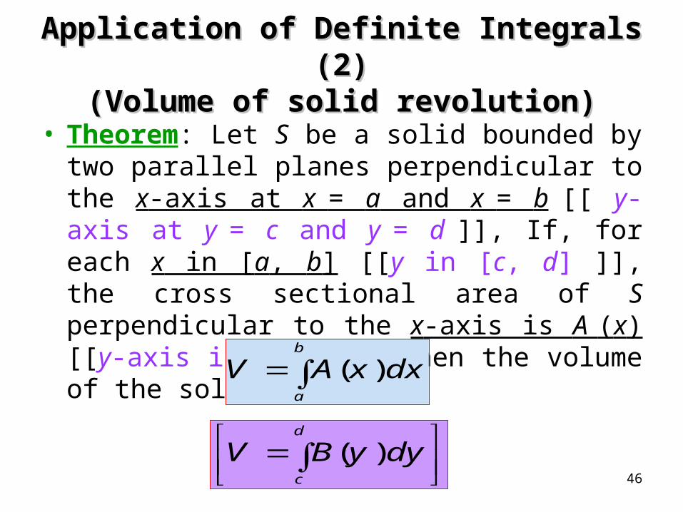
Application of Definite Integrals (2)Application of Definite Integrals (2)(Volume of solid revolution)(Volume of solid revolution)

• Theorem: Let S be a solid bounded by two parallel planes perpendicular to the x-axis at x = a and x = b [[ y-axis at y = c and y = d ]], If, for each x in [a, b] [[y in [c, d] ]], the cross sectional area of S perpendicular to the x-axis is A (x) [[y-axis is B(y) ]], then the volume of the solid is

( )

b

a

V A x dx

( )d

c

V B y dy

47

Solid RevolutionSolid Revolution• Let f be continuous and non negative in [a, b] and

let R be the region bounded by y = f (x) above x-axis between x = a and x = b. Then the solid generated by revolving the region R about the x-axis is such as require in the above theorem [each cross sectional area is a circular disk with radius f (x)]. Thus volume of the solid revolution is

2

( ) ( )

( )b

a

A x f x

V A x dx

48

Volume of a Cone (r, h)

-0.5 0 0.5 1 1.5 2 2.5 3 3.5-0.5

0

0.5

1

1.5

2Region bounded by y=x/2 above x-axis between 0 and 3

x-axis

y-a

xis

y=x/2

x=3

49

Volume of a Cone (r, h)

50

2 2 2

32 3 3

3 00

2 4

4 12 12

9 4

( ) ( ) / /

/ / /

/

x x

A x f x x x

V x dx x x

On the other hand, we know volume of a cone of radius r (=3/2) and height h (=3) is

3

2 2

3 0 3

2 3 2

3 3 2 3 3 9 4

/ /

/ ( / ) ( ) / /x

h

r x

V r h

51

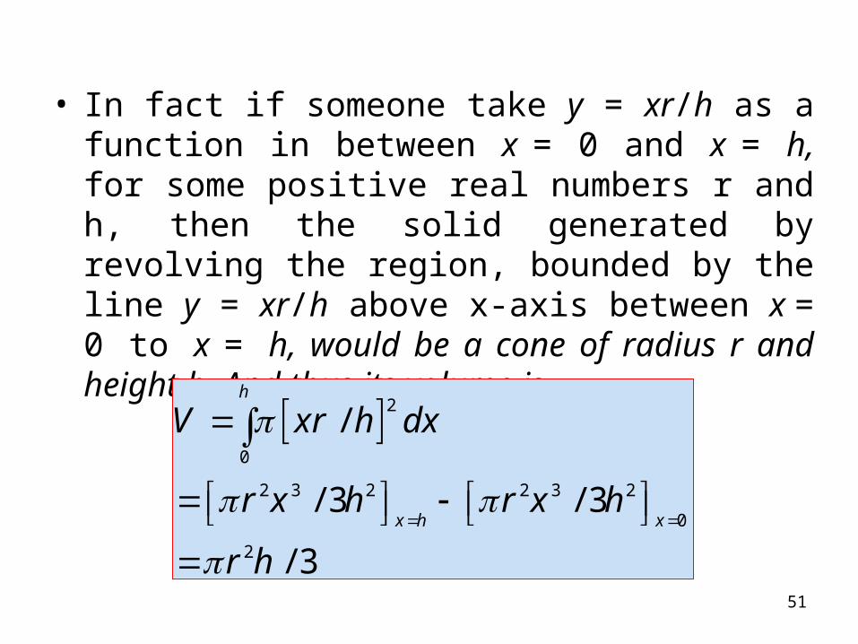
• In fact if someone take y = xr/h as a function in between x = 0 and x = h, for some positive real numbers r and h, then the solid generated by revolving the region, bounded by the line y = xr/h above x-axis between x = 0 to x = h, would be a cone of radius r and height h. And thus its volume is

20

2 3 2 2 3 2

0

2

3 3

3

/

/ /

/

h

x h x

V xr h dx

r x h r x h

r h

52

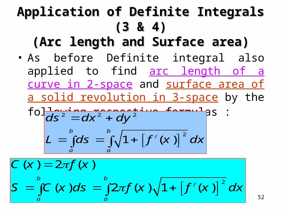
Application of Definite Integrals (3 & 4)Application of Definite Integrals (3 & 4)(Arc length and Surface area)(Arc length and Surface area)

• As before Definite integral also applied to find arc length of a curve in 2-space and surface area of a solid revolution in 3-space by the following respective formulas :

2 2 2

21

/ ( )b b

a a

ds dx dy

L ds f x dx

2

2

2 1

/

( ) ( )

( ) ( ) ( )b b

a a

C x f x

S C x ds f x f x dx

53

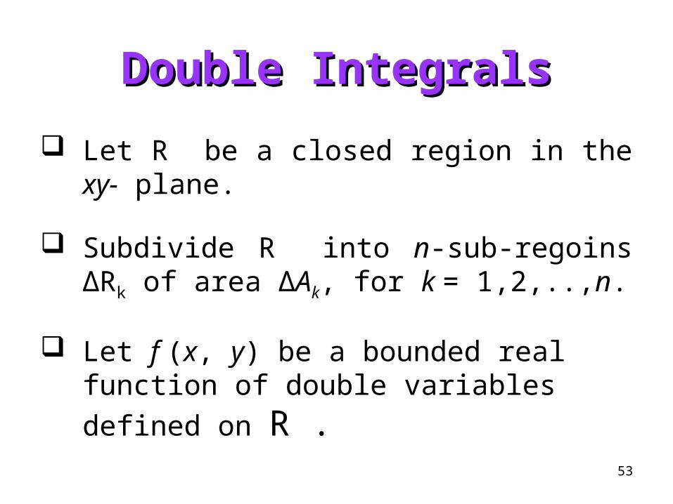
Double IntegralsDouble Integrals

Let R be a closed region in the xy- plane.

Subdivide R into n-sub-regoins ∆Rk of area ∆Ak, for k = 1,2,..,n.

Let f (x, y) be a bounded real function of

double variables defined on R .

54

Double IntegralsDouble Integrals

For each k = 1,2,…,n, Define

And then

Also for each k =1,2,…,n, choose

R( , )k k k

( ) sup { ( , ) : , }k k k

diam d p q p qR R R

1 2max { ( ) : , ,..., }k

diam k n R

55

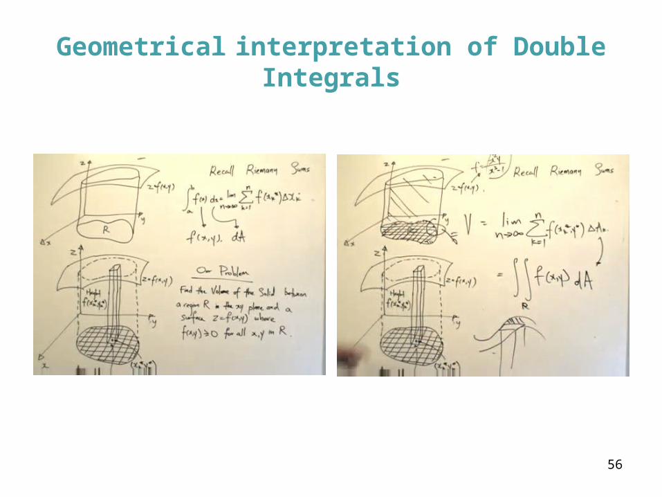
Geometrical interpretation of Double

Integrals

( , )k k

Elementary sub-region

∆R k of area ∆Ak

R

diam (∆Rk)

56

Geometrical interpretation of Double Integrals

57

Double IntegralsDouble Integrals

• Then the Double integral of f over the

region R is defined by

Provided the limits exist.

0 1

1

R

R

Or eqivalentlyby( , ) lim ( , )

( , ) lim ( , )

n

k k kk

n

k k kn k

f x y dA f A

f x y dA f A

58

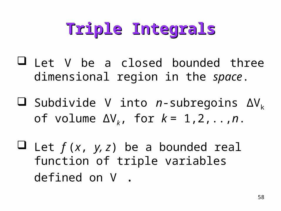
Triple IntegralsTriple Integrals

Let V be a closed bounded three dimensional region in the space.

Subdivide V into n-subregoins ∆Vk of volume ∆Vk, for k = 1,2,..,n.

Let f (x, y, z) be a bounded real function

of triple variables defined on V .

59

Triple IntegralsTriple Integrals

For each k = 1,2,…,n, Define

And then

Also for each k =1,2,…,n, choose

V( , , )k k k k

V V V( ) sup { ( , ) : , }k k k

diam d p q p q

1 2Vmax { ( ) : , ,... }k

diam k n

60

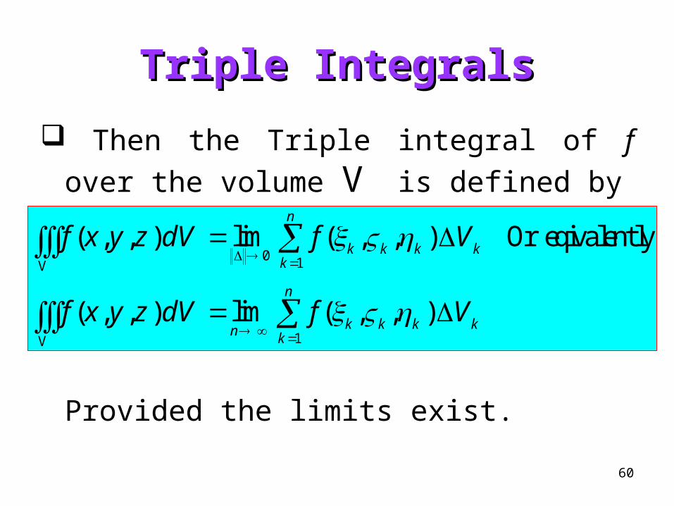
Triple IntegralsTriple Integrals

Then the Triple integral of f over the

volume V is defined by

Provided the limits exist.

0 1

1

V

V

Or eqivalently( , , ) lim ( , , )

( , , ) lim ( , , )

n

k k k kk

n

k k k kn k

f x y z dV f V

f x y z dV f V

61

Sufficient condition forSufficient condition forDouble and Triple integralsDouble and Triple integrals

• In both the cases of Double and Triple, we have mentioned that the multiple integral exists if the corresponding limit exists.

• And the limits exist if the functions are continuous on the corresponding regions.

• And all the properties of single integral hold here likely.

62

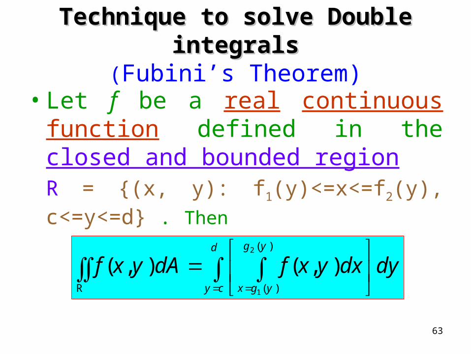
Technique to solve Double Technique to solve Double integralsintegrals

(Fubini’s Theorem)• Let f be a real continuous function

defined in the closed and bounded region

R = {(x, y): a<=x<=b, f1(x)<=y<=f2(x)} . Then

2

1

R

( )

( )

( , ) ( , )f xb

x a y f x

f x y dA f x y dy dx

63

Technique to solve Double Technique to solve Double integralsintegrals

(Fubini’s Theorem)• Let f be a real continuous function

defined in the closed and bounded regionR = {(x, y): f1(y)<=x<=f2(y), c<=y<=d} . Then

2

1

R

( )

( )

( , ) ( , )g yd

y c x g y

f x y dA f x y dx dy

64

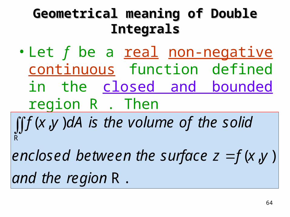
Geometrical meaning of Double IntegralsGeometrical meaning of Double Integrals

• Let f be a real non-negative continuous function defined in the closed and bounded region R . Then

R

R .

( , )

( , )

f x y dA is the volume of the solid

enclosed between the surface z f x y

and the region

65

• Let f be a real continuous function (non-negativity is not assured) defined in the closed and bounded region R . Then

R

algebraicsum( , )

,

.

f x y dA is the of the

volumes above and below the xy plane

treating volume abovethe xy plane as

positive and below the plane as negative

Geometrical meaning of Double IntegralsGeometrical meaning of Double Integrals

66

Application of Double Integrals (1)Application of Double Integrals (1)((Area of a regionArea of a region))

• Let R be a closed and bounded region in the xy-plane. Then

1

R

R ,

R .

dA is the voume of the solid enclosed

between the surface z and the region

which is in value nothing but the area of

the region

67

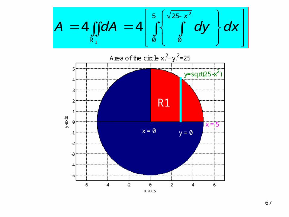
2

1

5 25

0 0

4 4

R

x

A dA dy dx

-6 -4 -2 0 2 4 6

-5

-4

-3

-2

-1

0

1

2

3

4

5

x-axis

y-ax

is

Area of the circle x.2+y.2=25

y=sqrt(25-x2)

x = 0 y = 0

R1

x = 5

68

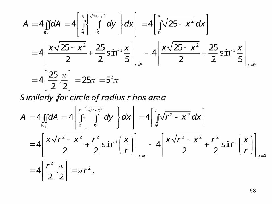
2

1

5 25 52

0 0 0

2 21 1

5 0

2

4 4 4 25

25 25 25 254 4

2 2 5 2 2 5

254 25 5

2 2

R

sin sin

.

x

x x

A dA dy dx x dx

x x x x x x

2 2

1

2 2

0 0 0

2 2 2 2 2 21 1

0

22

4 4 4

4 42 2 2 2

42 2

R

,

sin sin

. .

r r x r

x r x

Similarly for circleof radius r has area

A dA dy dx r x dx

x r x r x x r x r xr r

rr

69

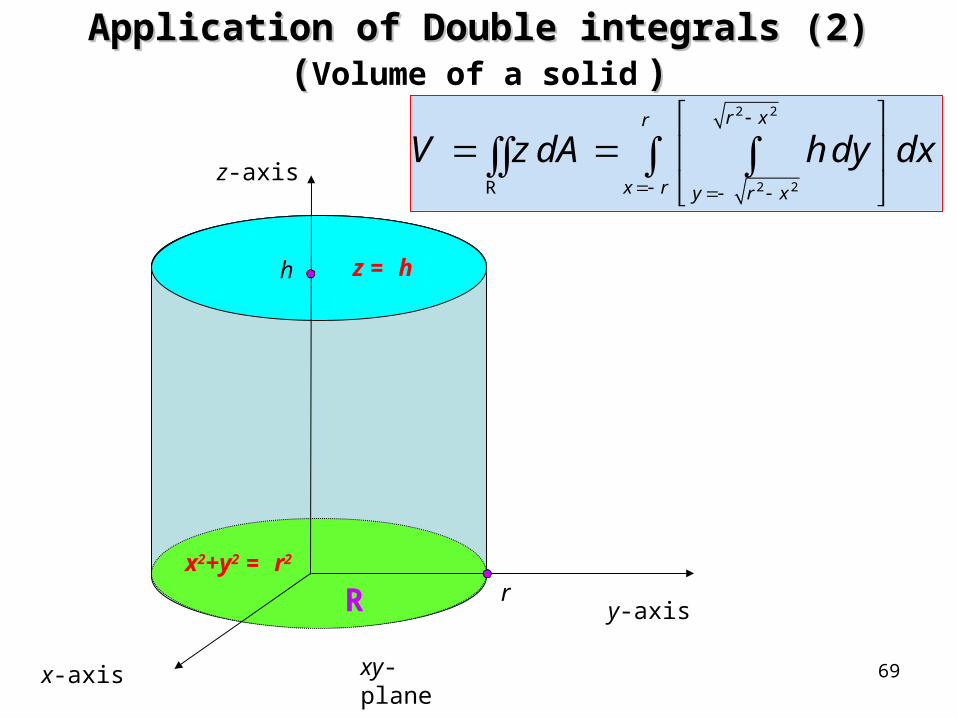
Application of Double integrals (2)Application of Double integrals (2)((Volume of a solid ))

x-axis

y-axis

z-axis

z = h

x2+y2 = r2

r

h

2 2

2 2

R

r xr

x r y r x

V zdA hdy dx

xy-plane

R

70

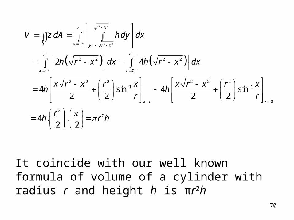
2 2

2 2

2 2 2 2

0

2 2 2 2 2 21 1

0

22

2 4

4 42 2 2 2

42 2

R

sin sin

. .

r xr

x r y r x

r r

x r x

x r x

V zdA hdy dx

h r x dx h r x dx

x r x r x x r x r xh h

r r

rh r h

It coincide with our well known formula of volume of a cylinder with radius r and height h is πr2h

71

Application of Double Integrals (3)Application of Double Integrals (3)(Mass of a lamina)(Mass of a lamina)

• If a lamina with continuous density function σ(x, y) occupies a region R in the xy-plane, then the mass M of the lamina is

R

( , )M x y dA

72

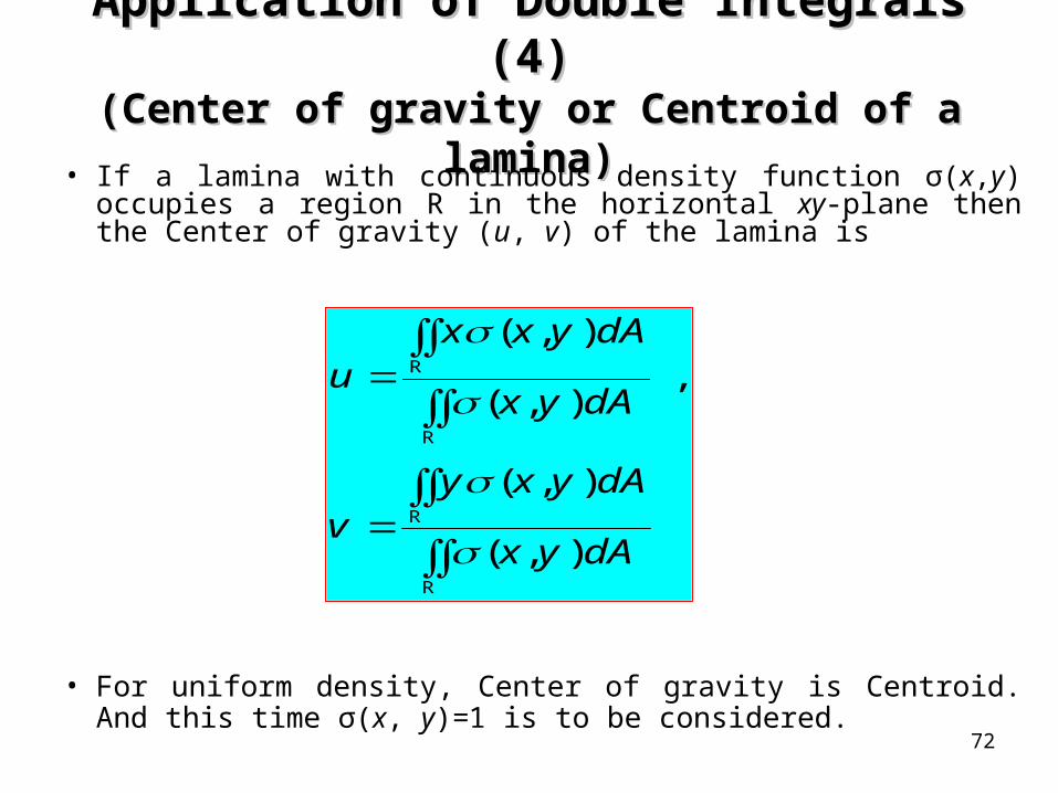
Application of Double Integrals (4)Application of Double Integrals (4)(Center of gravity or Centroid of a lamina)(Center of gravity or Centroid of a lamina)

• If a lamina with continuous density function σ(x,y) occupies a region R in the horizontal xy-plane then the Center of gravity (u, v) of the lamina is

• For uniform density, Center of gravity is Centroid. And this time σ(x, y)=1 is to be considered.

R

R

R

R

( , ),

( , )

( , )

( , )

x x y dAu

x y dA

y x y dAv

x y dA

73

Solving Techniques for Triple Solving Techniques for Triple IntegralsIntegrals

• Let G be a solid bounded above by the surface z = g1(x,y) and below by the surface z=g2(x,y), and R be the projection of G on the xy-plane. Also, say g1 and g2 are continuous on R , and f (x, y, z) is a function continuous on G, then

2

1

R

( , )

( , )

( , , ) ( , , )g x y

G z g x y

f x y z dV f x y z dz dA

74

Transformation of co-ordinates and Transformation of co-ordinates and JacobianJacobian

• Let T be a transformation from the uv-plane to the xy-plane defined by the equations x=x(u,v) and y=y(u,v), then the Jacobian J of T is

( , )( , )

( , )

x xx y u vJ u vu v y y

u v

75

Transformation of co-ordinates and JacobianTransformation of co-ordinates and Jacobian

• If the transformation x=x(u,v) and y=y(u,v), maps the region S in the uv-plane to the region R in the xy-plane and if the Jacobian J(u,v) is non-zero and does not change sign on S, then with appropriate restrictions on the transformation and the region it follows that

• Analogous for triple integrals

R S

( , ) ( ( , ), ( , )) ( , )xy uvf x y dA f x u v y u v J u v dA

( , , ) ( ( , , ), ( , , ), ( , , )) ( , , )xyz uvwG H

f x y z dV f x u v w y u v w z u v w J u v w dV

76

Applications of Triple Integrals (1)Applications of Triple Integrals (1)(Volume of a solid)(Volume of a solid)

• Let G be a solid bounded above by the surface z = g1(x,y) and below by the surface z = g2(x,y), and R be the projection of G on the xy-plane. Also, say g1 and g2 are continuous on R , then volume of the solid is

2

1

R

( , )

( , )

g x y

G z g x y

V dV dz dA

77

Volume of a sphere with radius r

2 2 2

2 2 2

2 2

2 2

2 2 2 2 2 2 2

2 2 2

22 2 2 2 2

0 0

2 2 2 2

0 0

3 22 2

2

2 2

4 2 2

22

3

R R

/

( )

( )

R x y

G z R x y

R R x R

x R ry R x

R R

r r

r

x y z R z R x y

V dV dz dA R x y dA

R x y dydx R r r dr d

R r r dr R r r dr

R r

3 22 2

0

33 22

2

3

2 42

3 3

/

/( ). . .

R rR r

RR

78

Applications of Triple Integrals (2)Applications of Triple Integrals (2)(Mass of a solid)(Mass of a solid)

• Let a solid with continuous density function σ (x, y, z) occupies a region G in the space, then mass M of the solid is

( , , )G

M x y z dV

79

Application of Triple Integrals (3)Application of Triple Integrals (3)((Center of gravity and centroid of a solidCenter of gravity and centroid of a solid))

• If a solid with continuous density function σ(x, y, z) occupies a region G in the space, then the center of gravity (u, v, w) of the solid is

• For uniform density, center of gravity is centroid. And this time σ(x, y, z)=1 is to be considered.

( , , ) ( , , ), ,

( , , ) ( , , )

( , , )

( , , )

G G

G G

G

G

x x y z dV y x y z dVu v

x y z dV x y z dV

z x y z dVw

x y z dV

80

Let C be a smooth (having smooth parametrization x = x (t), y = y (t), z = z (t) for a<=t<=b) curve in the 3-space joining the points P and Q.

Further, Let f (x, y, z) be a real function defined on C.

Line Integrals (for Scalar functions)

81

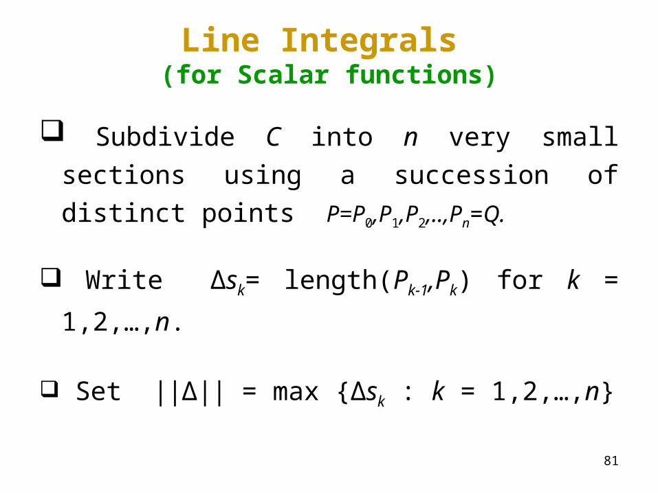
Line Integrals (for Scalar functions)

Subdivide C into n very small sections

using a succession of distinct points P=P0,P1,P2,..,Pn=Q.

Write ∆sk= length(Pk-1,Pk) for k = 1,2,…,n.

Set ||∆|| = max {∆sk : k = 1,2,…,n}

82

Line Integrals(for Scalar functions)

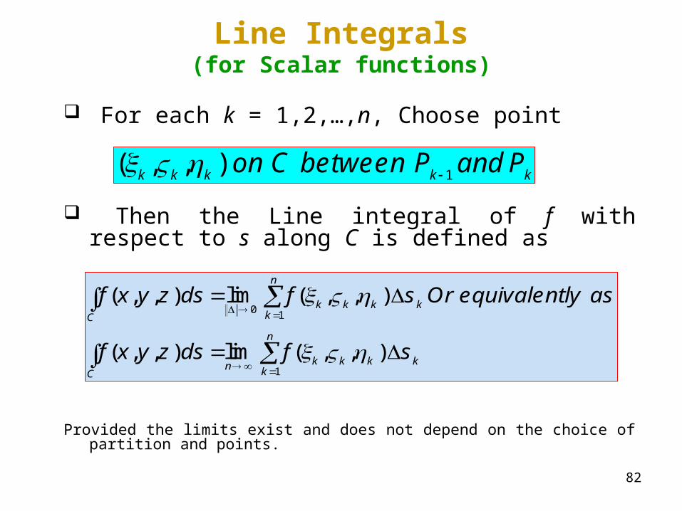
For each k = 1,2,…,n, Choose point

Then the Line integral of f with respect to s along C is defined as

Provided the limits exist and does not depend on the choice of partition and points.

1 ( , , )k k k k kon C between P and P

0 1

1

( , , ) lim ( , , )

( , , ) lim ( , , )

n

k k k kkC

n

k k k kn kC

f x y z ds f s Or equivalently as

f x y z ds f s

83

Geometric interpretation

P=P0

P1

P2

P3

Pn=Q

P4

P5

Pk

Pn-1

Pk-1

P1*(ξk, ζk, ηk)

P2*

P3*

P4*

P5*

Pk*

Pn*

C

∆sk

84

Evaluating technique of Line integrals

1

/ / *

*

( ) ( ) ( ) ( ) ; .

( ) ( ) .

, ( ( ), ( ), ( ))

[ , ],

( , , ) ( ( ), (

k

k

t

k k kt

k k

Let C be a curve inspacesmoothly parameterized by

t x t y t z t a t b Then

s r t dt r t t

Furthermore if f x t y t z t bea real valued

functiondefined on a b then

f x y z ds f x t y t

r i j k

1

2 2 2

* * / *

/

/ *

), ( )) ( )

( ( ), ( ), ( )) ( )

( )

n

k k kkC

b

a

k t t t

z t r t t

f x t y t z t r t dt

where r t x y z

85

Applications of Line Integrals (1) Applications of Line Integrals (1) (Mass of wire)(Mass of wire)

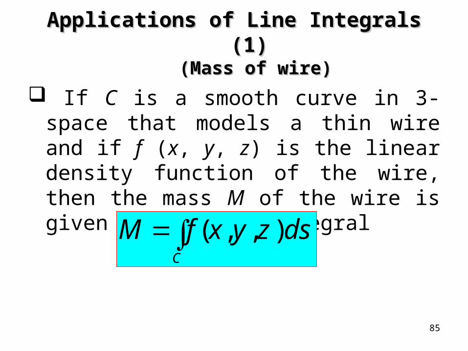
If C is a smooth curve in 3-space that models a thin wire and if f (x, y, z) is the linear density function of the wire, then the mass M of the wire is given by the line integral

( , , )C

M f x y z ds

86

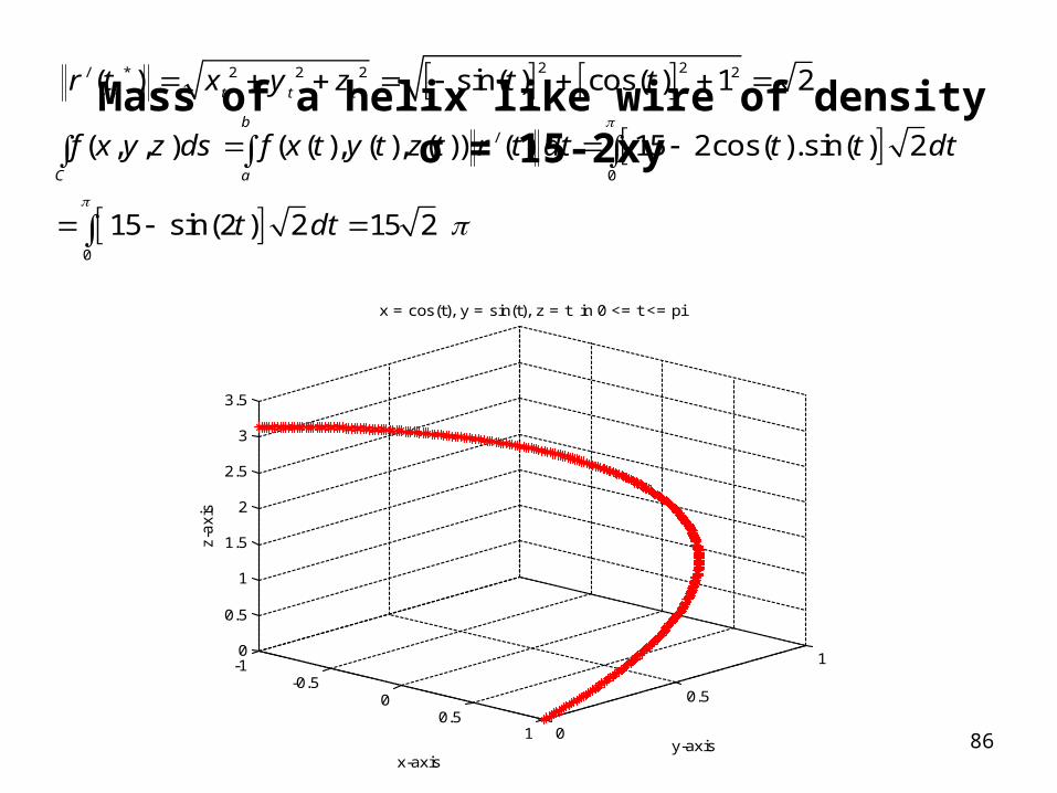
Mass of a helix like wire of density σ = 15-2xy

2 22 2 2 2

0

0

1 2

15 2 2

15 2 2 15 2

/ *

/

( ) sin( ) cos( )

( , , ) ( ( ), ( ), ( )) ( ) cos( ).sin( )

sin( )

k t t t

b

C a

r t x y z t t

f x y z ds f x t y t z t r t dt t t dt

t dt

-1-0.5

00.5

1 0

0.5

10

0.5

1

1.5

2

2.5

3

3.5

y-axis

x = cos(t), y = sin(t), z = t in 0 <= t <= pi

x-axis

z-a

xis

87

Applications of Line Integrals (2)Applications of Line Integrals (2)(Length of wire) (Length of wire)

If C is a smooth curve in 2-space. Then the length L of the curve is given by the line integral

C

L ds

88

Applications of Line Integrals (3)Applications of Line Integrals (3)(Area of sheet)(Area of sheet)

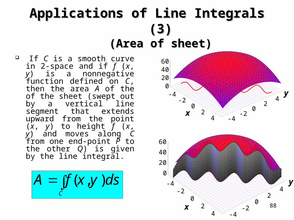
If C is a smooth curve in 2-space and if f (x, y) is a nonnegative function defined on C, then the area A of the of the sheet (swept out by a vertical line segment that extends upward from the point (x, y) to height f (x, y) and moves along C from one end-point P to the other Q) is given by the line integral.

( , )C

A f x y ds

604020

0y

42

0-2

-4x

42

0-2

-4

60

40

20

0

y4

20

-2-4

x4

20

-2-4

89

Applications of Line Integrals (4)Applications of Line Integrals (4)(Moments of Inertia)(Moments of Inertia)

Moments of inertia about the x-axis

Moments of inertia about the y-axis

Moments of inertia about the z-axis

2 2 ( , , )x

c

I y z f x y z ds

2 2 ( , , )x

c

I y z f x y z ds

2 2 ( , , )x

c

I y z f x y z ds

90

Line Integrals(for Vector fields)

• If C is a smooth oriented curve parameterized by

r=r(t)=x(t)i+y(t)j+z(t)k, and F=F1(x(t),y(t),z(t))i+F2(x(t),y(t),z(t))j+

F3(x(t),y(t),z(t))k is a continuous vector field over C, then the line

integral of F over C is

1 2 3 .C C

d Fdx F dy F dzF r

91

Theorem1. If F is conservative i.e. F = f for some f , then every

line integral of F will be independent of path and

where (x(a),y(a),z(a)) is the beginning of the curve and (x(b),y(b),z(b)) is the end of the path.

2. If every line integral of the form is independent of path, then F is conservative.

Corollary F is conservative if and only if

for any closed path lying inside the domain of F.

Cd F r

, , , ,C

d f x b y b z b f x a y a z a F r

0C

d F r

92

Applications of Line Integrals (4) Applications of Line Integrals (4) (Work done)(Work done)

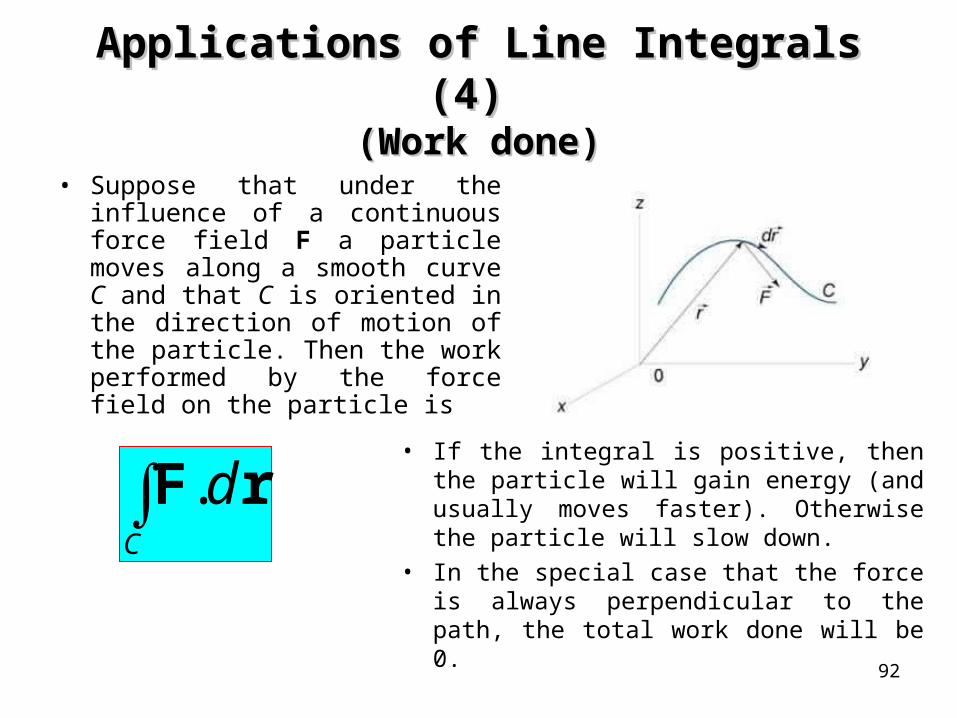
• Suppose that under the influence of a continuous force field F a particle moves along a smooth curve C and that C is oriented in the direction of motion of the particle. Then the work performed by the force field on the particle is

.C

dF r• If the integral is positive, then the particle

will gain energy (and usually moves faster). Otherwise the particle will slow down.

• In the special case that the force is always perpendicular to the path, the total work done will be 0.

93

• Find the work done moving once around an ellipse C in the xy-plane having center at the origin and semi major and semi minor axes 4 and 3 respectively with in a force field

F=(3x-4y+2z)i+(4x-2y-3z2)j+(2xz-4y2+z3)k

Soln: In the xy-plane z=0. Thus rewrite

F=(3x-4y)i+(4x-2y)j+(2xz-4y2)k and dr=dx i + dy j

And parameterized C as :

x=4 cos(t), y=3 sin(t), 0<=t<=2*pi.

94

2

0

2

0

2

0

3 4 4 2

3 4 4 3 4 4 4 2 3 3

48 16 6 3

48 30 48 15

. ( ) ( )

. .cos( ) . sin( ) ( cos( )) . .cos( ) . sin( ) ( sin( ))

cos( ) sin( ) . sin( ) ( )) cos( ) sin( ) . cos( ) ( )

.cos( ).sin( ) .sin

C C

t

t

t

W d x y dx x y dy

t t d t t t d t

t t t dt t t t dt

t t dt

F r

2

0

2 48 2 96( ) *t

t dt

Thus the Work done is given by the line integral

95

Ampere's Law

• The line integral of a magnetic field around a closed path C is equal to the total current flowing through the area bounded by the contour C. This is expressed by the formula

• Where is the vacuum permeability constant, equal to H/m.

0.C

d IB r0

96

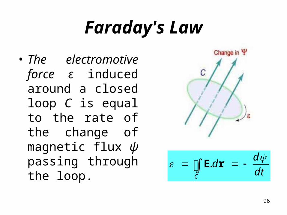
Faraday's Law

• The electromotive force ε induced around a closed loop C is equal to the rate of the change of magnetic flux ψ passing through the loop.

.C

dd

dt E r

97

Green’s Theorem• Let R be a simply connected

plane region bounded by a simple

closed piecewise smooth

counterclock-wise oriented curve

C. If F=F1(x,y)+F2(x,y) be a function

with component functions are

continuous and having continuous

partial derivatives on some region

containing R , then

1 2.C

F Fd dA

x y

F r

R

98

References

1. D V Widder (1961), Advanced Calculus, PHL Learning Private Ltd.

2. H Anton, I Bivens, S Davis (2008), Calculus, 8th edition, John

Willey and Sons.

3. MR Spigel, Theory and Problems of Advanced Calculus, SI

(Metric) Edition, Schaum’s Outline Series..

4. W Rudin (1976), Principles of Mathematical Analysis, 3rd Edition,

Mcgraw-Hill International

5. www.google.com

99

THANKS THANKS EVERYBODYEVERYBODY

QUESTIONS???QUESTIONS???

THANKS THANKS EVERYBODYEVERYBODY

QUESTIONS???QUESTIONS???