propagation measurements at 2.4 ghz inside a university

Propagation Measurements at 2.4 GHz Inside a University Building and Estimation of Saleh-

Valenzuela Parameters

Zoran Blažević, Igor Zanchi and Ivan Marinović

Abstract: In this paper we analyze measurements conducted in an indoor environment of our university building at a central frequency of 2.4 GHz in terms of the Saleh-Valenzuela channel. The channel parameters are extrapolated by processing the power-delay profiles measured by a vector network analyzer. Final adjustments of the parameters are obtained by comparison of simulated and measured delay-spread cumulative density functions, where a quite good agreement between the two is obtained. The predictions of the coherence bandwidth are satisfactory as well. We also considered some extensions to the original form of the model and concluded that the one that would be worthy to apply is the one that, besides temporal, incorporates also spatial information about the channel, whereas other modifications are found to be unnecessary or even unjustified for evaluation of this indoor propagation scenario. Index terms: indoor radio-propagation, delay-spread, coherence bandwidth, Saleh-Valenzuela channel model

I. INTRODUCTION The ongoing development of radio transmission techniques offers great possibilities for wireless communication at the velocity of light among the users and communication networks. As generally the quantity of information exchanged through the networks and the number of services increase continuously with time as well as the number of users, the demands for the bandwidth increase accordingly. This pushes the technology to shift toward higher frequencies, imposing new requests to radio engineers regarding channel modeling, modulation and coding. Special challenge is modeling indoor radio channels, which is the issue of many research papers, e.g. [1-14]. Naturally, the development and minimization of computers make the wireless local-area networks or wireless internet much more demanding in a sense of the need for much higher data rates than it was at the beginning. Consequently, as the communication traffic increases continuously as well as the quantity of data that can be stored, retrieved or exchanged via these networks, they become of great importance to everyday

research, business and life in general. The latest development is the application of the ultrawideband (UWB) technology in indoor radio networks. Regardless of the type of a wireless network, the key to the optimum design is to find an adequate description of the propagation environment within the available bandwidth, which then enables us to evaluate or develop best procedures in order to meet the demanded quality of service. This task is not at all easy, because the accurate physical description of real radio channels based on the Maxwell equations is usually too complicate to deal with. That is why many approximate methods, such as ray-tracing, "knife-edge" or geometrical optic, are in common use. However, depending on the scenario, they do not always satisfy us either from the standpoint of computational complexity or due to the accuracy. Namely, in indoor environments the multipath propagation is usually very complicated and coupled with attenuation of the electromagnetic waves traversing obstacles such as interior walls and furniture. On the other hand statistical models based on measurements, although they say little or nothing about the physic governing a radio transmission, are very useful in predicting the system performances in many instances. Therefore, if they are combined with certain solid physical facts that can be established for the examined propagation scenarios they become the most reliable tools for the development of a radio network. A very useful and reliable semi-statistical model has been developed for indoor environments in [1] by Saleh and Valenzuela. Saleh-Valenzuela (SV) model provides the radio channel characterization based on four statistical parameters of a double-Poisson process of clustering of multipath rays that is evident from transmission response measurements. The model is adopted by IEEE 802.14.4a working group for the estimations of indoor UWB radio systems as a reference channel model [6-8], which speaks more than enough about its efficiency and popularity. There are also interesting extensions to the model made by other authors [2-6, 8], who import various additional parameters in order to refine the model and improve the usage. Namely, the original form of the SV model provides a description of only temporal characteristics of the channel, whereas the spatial properties can be assessed by measuring the arrival angle data using directional antennas as has been done in [2-4]. It has been shown there that the clustering effect stretches to the angle dimension as well as the time, and stressed that the joint temporal-spatial characteristics

Manuscript received May 9, 2007 and revised June 21, 2007. This

work has been partially supported by Ministry of Science and Technology, Croatia, within frame of the project No. 023-0361566-1613 "Propagation Factors in Radio Networks Planning" in 2007.

Authors are with the University of Split, Faculty of Electrical Engineering, Mechanical Engineering and Naval Architecture, Split, Croatia (e-mail: zblaz, izanchi, [email protected]).

JOURNAL OF COMMUNICATIONS SOFTWARE AND SYSTEMS, VOL. 3, NO. 2, JUNE 2007 387

1845-6421/07/7099 © 2007 CCIS

99

FESB

Typewritten Text

Original scientific paper

may be quite important to the radio systems that employ a spatial diversity. Also, as is clearly depicted in [2, 4], the analysis of the two-dimensional data greatly improves and makes the identification of clusters significantly easier, because the clusters emanating from various angles of arrivals often overlap in the time dimension. Besides, the application of a directional antenna improves the signal-to-noise ratio (SNR) at the receiving point. However, the number of measurements increases, the measurement procedure is complicated further and the demands on the measuring equipment are harder to meet. Furthermore, the second abbreviation in the SV model is made by supposing that all clusters within a response have the same power-delay time constants for the rays, which has been the base for another useful extension of the original SV model in the scenario of an industrial indoor environment in [5]. The next example of modification of the SV model is the Split-Poisson model proposed in [6], which assumes a fixed number of clusters instead of a Poisson random number of clusters. This model is compared for the specific scenario to other statistical models including SV in [7], where it was found that it outperforms other examined models in predicting the bit-error rates for a Rake receiver with a number of fingers greater than two. Finally, in [8], a comprehensive model for UWB channels that combines several modifications of the SV model is presented. In this paper we present the analysis of wideband radio measurements at 2.4 GHz conducted inside a university building. Besides the comparison with results and conclusions presented in other references, it is our basic intention to show that by a relatively straightforward procedure based on a limited subset of measurements one may achieve a proper channel evaluation by the original form of the SV model. Namely, from the inspection of our measured results and from the comparison with the simulated results, we deduce that the modifications introduced in [5, 6] are unjustified and unnecessary for this indoor propagation example. On the other hand, although by processing the information about spatial characteristics of the channel a more sophisticated analysis can be conducted, we manage to achieve a very good match of simulated to the measured delay-spread cumulative density function (CDF) without it and, although conservative to a degree, satisfactory predictions of the coherence bandwidth CDF estimated by measurements. Therefore, we conclude that in this scenario the original form of SV model performs quite well and that executing more complicated measurements by directional antennas is not always of a decisive importance for the evaluation of the channel. The paper is organized as follows. The indoor propagation description by the SV model will be briefly introduced in Sec. II, along with the channel parameters important for the evaluation of the channel. In Sec. III the examined propagation environment and measurement setup will be described. In Sec. IV we shall present the analysis of the measurements by the discrete SV model what will be discussed upon. This is followed by conclusions in Sec. V.

II. INDOOR PROPAGATION CHANNEL MODELING

As the SV model (as well as the extensions to the model) has already been depicted in many references, we shall only

briefly describe the main characteristics of the model and stress some of the details important to the completeness and clearness of the paper. The fundamental idea behind this widely accepted model comes from the observation of the impulse responses h(t) of indoor radio channels, where it has been noted that the arrival of the total electromagnetic energy radiated by a transmitter is manifested in the measured power-delay profiles (PDP) Ph(t) = |h(t)|2 in the form of more or less distinguishable exponentially decaying clusters of rays that may be described statistically. Under the assumption of a wide-sense stationary (WSS) channel, an indoor impulse response as a function of time t can then be represented as [1]:

( ) ( )0 0

kljkl l kl

l kt g e t Tφ δ τ

∞ ∞

= =

= − −∑∑h , (1)

where the arrival time of the first ray within the lth cluster (the cluster arrival time) is denoted as Tl (with T0 = 0), and the arrival time of the kth ray within the lth cluster is denoted as τkl, taking that for the first ray within it is set to τ0l = 0. The both arrival times Tl and τkl are taken to be Poisson processes with some fixed rates Λ and λ, respectively. The notation gkl represents the path gain of the kth ray within the lth cluster, for which has been supposed by the model in [1] to be independent positive Rayleigh (or alternatively log-normally distributed) random variables with the mean square values 2

klg being monotonically decreasing functions of the arrival times Tl and τkl of the form:

( )2 2 2 γ00,

kllT

kl l klg g T g e eτ

τ−− Γ= = ⋅ , (2)

where Γ and γ are power-delay time constants for the clusters and the rays, respectively, and ( )2 2

00 0,0g g= is the average power gain of the first ray of the first cluster. The phase φkl is assumed to be a statistically independent random variable uniformly distributed over [0, 2π). The ultimate goal of the double-Poisson SV modeling is to find a satisfactory estimation of the values of parameters Λ, λ, Γ and γ that should be sufficient to adequately characterize a given indoor propagation environment in a statistical sense. The SV model with properly determined parameters can then be applied in simulations of a digital radio system performing in given conditions. The final adjustment (if necessary) and the accuracy test are usually performed by the comparison of measured and simulated delay-spread CDFs. The delay-spread σ is the standard deviation of a PDP calculated as:

2

2 1

0 0

m mm m

σ⎛ ⎞

= − ⎜ ⎟⎝ ⎠

, (3)

where mi is the ith moment of the PDP:

( )0

, 0,1,2,...ii hm t P t dt i

∞

= =∫ . (4)

388 JOURNAL OF COMMUNICATIONS SOFTWARE AND SYSTEMS, VOL. 3, NO. 2, JUNE 2007100

However, as pointed out in a number of references (e.g. [1, 17]), the delay-spread can be in certain conditions only a crude measure of channel frequency selectivity, and is not always the best tool for predicting the system performances. The parameter that can be used to evaluate precisely the time distortion of a wideband signal transmitted through the radio channel is the coherence bandwidth of the channel. It can be defined [9-11, 15-17] as the frequency separation ∆f at which the absolute of the channel frequency correlation function Rh that can be calculated via the Fourier Transform as:

( ) ( ) ( )2

0

j f th hf P t e dtπ

∞− ∆∆ = ∫R , (5)

drops below the autocorrelation threshold C (that is a parameter of receiver) for the first time. And although an explicit relationship between the coherence bandwidth and delay-spread does not exist, it is a proved fact that there is a significant correlation between the two (to the authors' knowledge in every examined indoor and outdoor propagation environment) and that there is an inverse proportionality between the trends of these values. A lower bound for the coherence bandwidth of a WSS channel is derived in [15] as:

minarccos

2CCB

πσ= . (6)

It is the exact value of the coherence bandwidth that corresponds to the two-path channel model in which the receiver collect equal amounts of electromagnetic energy via the both radio paths separated in time by 2σ. Beside these wideband parameters important for the estimation of the channel throughput, the most essential information about any radio channel is certainly the power-distance law, which can be presented in the form n

meanG d −∼ . It describes the decreasing of the mean power with the antenna separation d and can be used for a rough estimation of the radius of the influence of the transmitter. In order to derive the path-loss exponent n as the first parameter of the SV model, we define the relative attenuation L in decibels at a distance d from the transmitter as in [1, 7]:

( ) ( )1m

10logG d

L dG

= − , (7)

where G(d) is the total multipath power-gain calculated by (4) as the ratio of the null moment of the measured PDP and the null moment of the transmitted waveform. G1m = G(d = 1m) is the total path-gain at one meter distance between the used antennas with gains Gt and Gr, and can be reasonably accurately estimated by the Fris equation:

2

1m04t r

cG G Gfπ

⎛ ⎞= ⎜ ⎟

⎝ ⎠, (8)

where f0 is the central frequency of the band and c is the velocity of light.

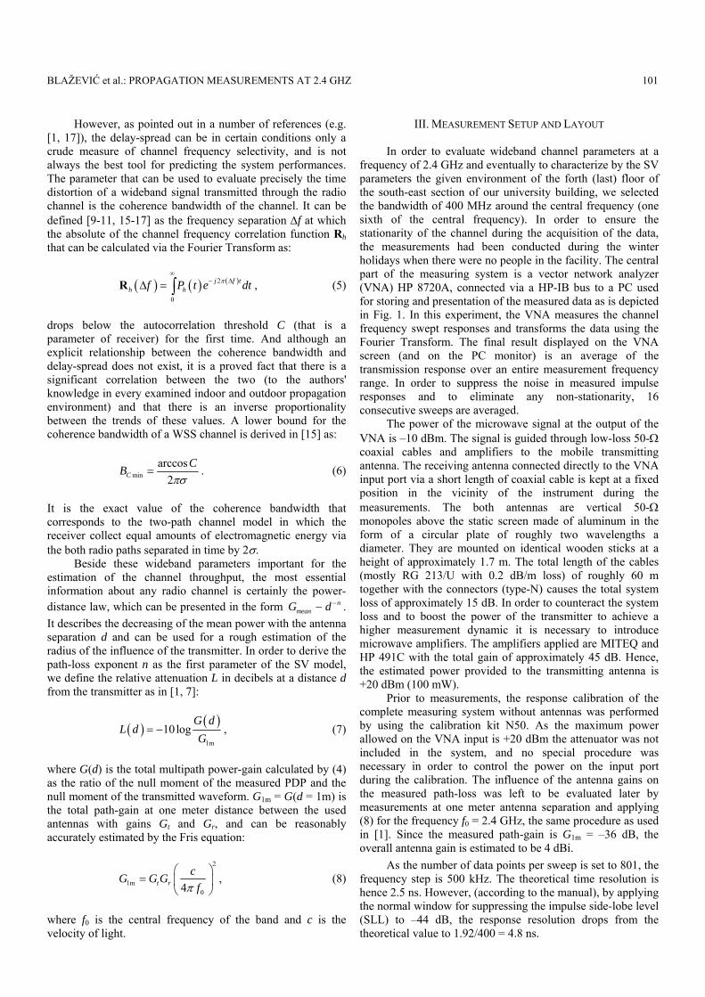
III. MEASUREMENT SETUP AND LAYOUT In order to evaluate wideband channel parameters at a frequency of 2.4 GHz and eventually to characterize by the SV parameters the given environment of the forth (last) floor of the south-east section of our university building, we selected the bandwidth of 400 MHz around the central frequency (one sixth of the central frequency). In order to ensure the stationarity of the channel during the acquisition of the data, the measurements had been conducted during the winter holidays when there were no people in the facility. The central part of the measuring system is a vector network analyzer (VNA) HP 8720A, connected via a HP-IB bus to a PC used for storing and presentation of the measured data as is depicted in Fig. 1. In this experiment, the VNA measures the channel frequency swept responses and transforms the data using the Fourier Transform. The final result displayed on the VNA screen (and on the PC monitor) is an average of the transmission response over an entire measurement frequency range. In order to suppress the noise in measured impulse responses and to eliminate any non-stationarity, 16 consecutive sweeps are averaged. The power of the microwave signal at the output of the VNA is –10 dBm. The signal is guided through low-loss 50-Ω coaxial cables and amplifiers to the mobile transmitting antenna. The receiving antenna connected directly to the VNA input port via a short length of coaxial cable is kept at a fixed position in the vicinity of the instrument during the measurements. The both antennas are vertical 50-Ω monopoles above the static screen made of aluminum in the form of a circular plate of roughly two wavelengths a diameter. They are mounted on identical wooden sticks at a height of approximately 1.7 m. The total length of the cables (mostly RG 213/U with 0.2 dB/m loss) of roughly 60 m together with the connectors (type-N) causes the total system loss of approximately 15 dB. In order to counteract the system loss and to boost the power of the transmitter to achieve a higher measurement dynamic it is necessary to introduce microwave amplifiers. The amplifiers applied are MITEQ and HP 491C with the total gain of approximately 45 dB. Hence, the estimated power provided to the transmitting antenna is +20 dBm (100 mW). Prior to measurements, the response calibration of the complete measuring system without antennas was performed by using the calibration kit N50. As the maximum power allowed on the VNA input is +20 dBm the attenuator was not included in the system, and no special procedure was necessary in order to control the power on the input port during the calibration. The influence of the antenna gains on the measured path-loss was left to be evaluated later by measurements at one meter antenna separation and applying (8) for the frequency f0 = 2.4 GHz, the same procedure as used in [1]. Since the measured path-gain is G1m = –36 dB, the overall antenna gain is estimated to be 4 dBi. As the number of data points per sweep is set to 801, the frequency step is 500 kHz. The theoretical time resolution is hence 2.5 ns. However, (according to the manual), by applying the normal window for suppressing the impulse side-lobe level (SLL) to –44 dB, the response resolution drops from the theoretical value to 1.92/400 = 4.8 ns.

BLAŽEVIĆ et al.: PROPAGATION MEASUREMENTS AT 2.4 GHZ 389101

<

VNA HP 8720A

6 8 10 12 14 16 18 20-140

-130

-120

-110

-100

-90

-80

-70

-60

Tim e-delay (ns )

Pat

h-lo

ss (d

B)

S IM U LA TIO N M E A S U RE M E NT

Rx

Tx OMNI ANTENNA

OMNI ANTENNA

6 8 10 12 14 1 6 18 20-15 0

-14 0

-13 0

-12 0

-11 0

-10 0

-9 0

-8 0

-7 0

-6 0

HP-IB

>HP 493C

MITEQ

LONG COAXIAL CABLE aprox. 50 m

SHORT COAXIAL CABLE

Fig. 1. Measurement setup

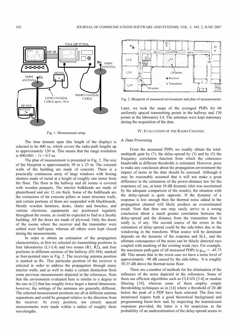
The time domain span (the length of the display) is selected to be 400 ns, which covers the radio-path lengths up to approximately 120 m. This means that the range resolution is 400/(801 – 1) = 0.5 ns. The plan of measurement is presented in Fig. 2. The size of the blueprint is approximately 50 m x 25 m. The external walls of the building are made of concrete. There is a practically continuous array of large windows with boxing shutters made of metal at a height of roughly one meter from the floor. The floor in the hallway and all rooms is covered with wooden parquets. The interior bulkheads are made of plasterboard and are 12 cm thick. Some of the bulkheads are the extensions of fat concrete pillars or inner structure walls, and certain portions of them are suspended with blackboards. Mostly wooden furniture, desks, chairs and benches, and various electronic equipments are positioned regularly throughout the rooms, as could be expected to find in a faculty building. All the doors are made of plywood. Only the doors of the rooms where the receiver and the transmitter were settled were half-open, whereas all others were kept closed during the measurements. In order to obtain an estimation of the propagation characteristics, at first we selected six transmitting positions in four laboratories (L1-L4) and two rooms (R1, R2), and four positions in different sections of the hallway (H1-H4), marked as four-pointed stars in Fig. 2. The receiving antenna position is marked as Rx. This particular position of the receiver is selected in order to address the propagation through many interior walls, and as well to make a certain distinction from some previous measurements depicted in the references. Note that the environment evaluated here is similar to a degree to the one in [1] that has roughly twice larger a lateral dimension; however, the settings of the antennas are generally different. The selected measurement positions are all at different antenna separations and could be grouped relative to the direction from the receiver. At every position, ten closely spaced measurements were made within a radius of roughly three wavelengths.

130 points

60 points

Receiver

Transmitter

Rx R1R2

H4

H1

H2 H3

L1

L2

L3 L4

Fig. 2. Blueprint of measured environment and plan of measurements Later, we took the snaps of the averaged PDPs for 60 uniformly spaced transmitting points in the hallway and 130 points in the laboratory L4. The antennas were kept stationary during the acquisition of the data.

IV. EVALUATION OF THE RADIO CHANNEL A. Data Processing From the measured PDPs we readily obtain the total-multipath gain by (7), the delay-spread by (3) and by (5) the frequency correlation function from which the coherence bandwidth at different thresholds is estimated. However, prior to make any conclusion about the propagation environment the impact of noise in the data should be assessed. Although it may be reasonably assumed that it will not make a great difference in the estimation of the power-distance law for the responses of, say, at least 10 dB dynamic (this was ascertained by the adequate comparison of the results), the situation with the delay-spread is quite opposite. If the dynamic of a response is low enough then the thermal noise added in the propagation channel will likely produce an overestimated result. Note that then one may easily arrive to a wrong conclusion about a much greater correlation between the delay-spread and the distance from the transmitter than it really is, if any. The second source of the errors in the estimation of delay-spread could be the side-lobes due to the windowing in the transform. What source will be dominant depends on the dynamic of the response and SLL, and the ultimate consequence of the noise can be falsely detected rays coupled with masking of the existing weak rays. For example, the maximum path-gain of all measured PDPs is gmax = –45.75 dB. This means that in the worst case we have a noise level of approximately –90 dB caused by the side-lobes. It is roughly 30-35 dB above the thermal noise floor. There are a number of methods for the elimination of the influence of the noise depicted in the references. Some of them use efficient algorithms such as CLEAN [2-4] or median filtering [10], whereas some of them employ simple thresholding techniques as in [14] where a threshold of 20 dB below the peak of a PDP have been selected. The first two mentioned require both a good theoretical background and programming know-how and, by inspecting the transmission responses provided, the latter is a bit suspicious as the probability of an underestimation of the delay-spread seems to


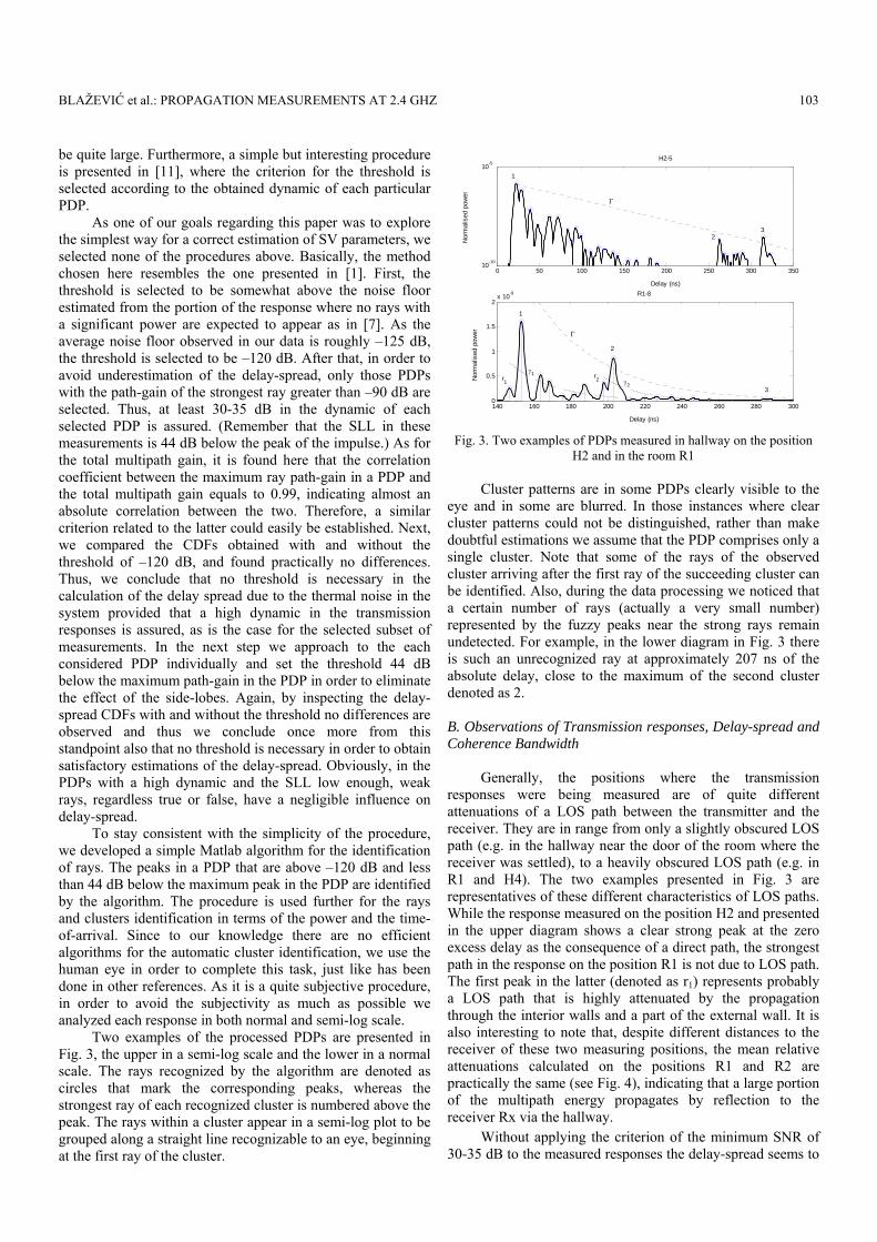
be quite large. Furthermore, a simple but interesting procedure is presented in [11], where the criterion for the threshold is selected according to the obtained dynamic of each particular PDP. As one of our goals regarding this paper was to explore the simplest way for a correct estimation of SV parameters, we selected none of the procedures above. Basically, the method chosen here resembles the one presented in [1]. First, the threshold is selected to be somewhat above the noise floor estimated from the portion of the response where no rays with a significant power are expected to appear as in [7]. As the average noise floor observed in our data is roughly –125 dB, the threshold is selected to be –120 dB. After that, in order to avoid underestimation of the delay-spread, only those PDPs with the path-gain of the strongest ray greater than –90 dB are selected. Thus, at least 30-35 dB in the dynamic of each selected PDP is assured. (Remember that the SLL in these measurements is 44 dB below the peak of the impulse.) As for the total multipath gain, it is found here that the correlation coefficient between the maximum ray path-gain in a PDP and the total multipath gain equals to 0.99, indicating almost an absolute correlation between the two. Therefore, a similar criterion related to the latter could easily be established. Next, we compared the CDFs obtained with and without the threshold of –120 dB, and found practically no differences. Thus, we conclude that no threshold is necessary in the calculation of the delay spread due to the thermal noise in the system provided that a high dynamic in the transmission responses is assured, as is the case for the selected subset of measurements. In the next step we approach to the each considered PDP individually and set the threshold 44 dB below the maximum path-gain in the PDP in order to eliminate the effect of the side-lobes. Again, by inspecting the delay-spread CDFs with and without the threshold no differences are observed and thus we conclude once more from this standpoint also that no threshold is necessary in order to obtain satisfactory estimations of the delay-spread. Obviously, in the PDPs with a high dynamic and the SLL low enough, weak rays, regardless true or false, have a negligible influence on delay-spread. To stay consistent with the simplicity of the procedure, we developed a simple Matlab algorithm for the identification of rays. The peaks in a PDP that are above –120 dB and less than 44 dB below the maximum peak in the PDP are identified by the algorithm. The procedure is used further for the rays and clusters identification in terms of the power and the time-of-arrival. Since to our knowledge there are no efficient algorithms for the automatic cluster identification, we use the human eye in order to complete this task, just like has been done in other references. As it is a quite subjective procedure, in order to avoid the subjectivity as much as possible we analyzed each response in both normal and semi-log scale. Two examples of the processed PDPs are presented in Fig. 3, the upper in a semi-log scale and the lower in a normal scale. The rays recognized by the algorithm are denoted as circles that mark the corresponding peaks, whereas the strongest ray of each recognized cluster is numbered above the peak. The rays within a cluster appear in a semi-log plot to be grouped along a straight line recognizable to an eye, beginning at the first ray of the cluster.

0 50 100 150 200 250 300 35010-10

10-5H2-5

Delay (ns)

Nor

mal

ised

pow

er

140 160 180 200 220 240 260 280 3000

0.5

1

1.5

2x 10-9 R1-8

Delay (ns)

Nor

mal

ised

pow

er

1

2 3

Γ

Γ

γ1

γ2

1

2

3

r1 r2

Fig. 3. Two examples of PDPs measured in hallway on the position

H2 and in the room R1 Cluster patterns are in some PDPs clearly visible to the eye and in some are blurred. In those instances where clear cluster patterns could not be distinguished, rather than make doubtful estimations we assume that the PDP comprises only a single cluster. Note that some of the rays of the observed cluster arriving after the first ray of the succeeding cluster can be identified. Also, during the data processing we noticed that a certain number of rays (actually a very small number) represented by the fuzzy peaks near the strong rays remain undetected. For example, in the lower diagram in Fig. 3 there is such an unrecognized ray at approximately 207 ns of the absolute delay, close to the maximum of the second cluster denoted as 2. B. Observations of Transmission responses, Delay-spread and Coherence Bandwidth Generally, the positions where the transmission responses were being measured are of quite different attenuations of a LOS path between the transmitter and the receiver. They are in range from only a slightly obscured LOS path (e.g. in the hallway near the door of the room where the receiver was settled), to a heavily obscured LOS path (e.g. in R1 and H4). The two examples presented in Fig. 3 are representatives of these different characteristics of LOS paths. While the response measured on the position H2 and presented in the upper diagram shows a clear strong peak at the zero excess delay as the consequence of a direct path, the strongest path in the response on the position R1 is not due to LOS path. The first peak in the latter (denoted as r1) represents probably a LOS path that is highly attenuated by the propagation through the interior walls and a part of the external wall. It is also interesting to note that, despite different distances to the receiver of these two measuring positions, the mean relative attenuations calculated on the positions R1 and R2 are practically the same (see Fig. 4), indicating that a large portion of the multipath energy propagates by reflection to the receiver Rx via the hallway. Without applying the criterion of the minimum SNR of 30-35 dB to the measured responses the delay-spread seems to


be significantly correlated with the antenna separation, as the calculated correlation coefficient between the two is 0.64. The maximum delay-spread in that case is 75 ns, and it is noted that the highest values of the delay spread are tied to great path-loss exclusively. But, after rejection of all the responses that do not match the criterion, the correlation coefficient drops to less than 0.4, indicating a weak correlation. The maximum delay-spread is now approximately 50 ns, which is practically the same as noted in [1, 12]. On the other hand, the median value observed here of approximately 30 ns is 4-5 ns greater than the one obtained in [1, 12]. However, the correlation between the delay-spread and the distance from the transmitter should not be totally neglected in environments with obstructed radio-paths, because it can be reasonably assumed that the power of the strongest rays decays with the distance much faster than the power of weak rays with long excess delays. If so, these weak rays could influence the delay-spread more as the antenna separation increases. A more exhaustive analysis of this can be found in [12]. Nonetheless, it can be stated firmly for this scenario that the delay-spread is tied mostly to the local surroundings of the antennas and not the antenna separation, similarly as deduced in [1] or [13]. A further inspection of the measured results showed that not a single value of the coherence bandwidth lies below the theoretical bound (6) (this is not the case in [10]). The relatively high values of the coherence bandwidths (say more than 25 MHz for the threshold of 1/√2) are at positions in the hallway with only a lightly obscured LOS path, at which also the measured delay-spread is generally lower than in the rest of the environment. There is a noticeable correlation coupled with an inverse proportionality between the delay-spread and coherence bandwidth regardless of the correlation threshold C, as can be deduced from the data listed in table 1.

TABLE 1. CORRELATION ρ BETWEEN DELAY-SPREAD AND COHERENCE BANDWIDTH AT DIFFERENT THRESHOLD LEVELS C

C 0.9 1/√2 0.5 1/e ρ –0.70 –0.66 –0.64 –0.62

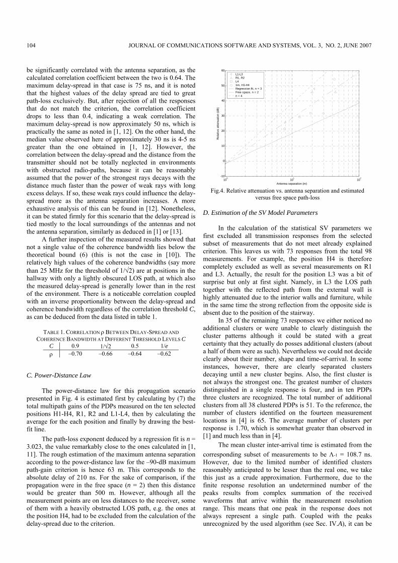
C. Power-Distance Law The power-distance law for this propagation scenario presented in Fig. 4 is estimated first by calculating by (7) the total multipath gains of the PDPs measured on the ten selected positions H1-H4, R1, R2 and L1-L4, then by calculating the average for the each position and finally by drawing the best-fit line. The path-loss exponent deduced by a regression fit is n = 3.023, the value remarkably close to the ones calculated in [1, 11]. The rough estimation of the maximum antenna separation according to the power-distance law for the –90-dB maximum path-gain criterion is hence 63 m. This corresponds to the absolute delay of 210 ns. For the sake of comparison, if the propagation were in the free space (n = 2) then this distance would be greater than 500 m. However, although all the measurement points are on less distances to the receiver, some of them with a heavily obstructed LOS path, e.g. the ones at the position H4, had to be excluded from the calculation of the delay-spread due to the criterion.

100 101 102-10

0

10

20

30

40

50

60

Antenna separation (m)

Rel

ativ

e at

tenu

atio

n (d

B)

L1-L3R1, R2L41m, H1-H4Regression fit, n = 3Free space, n = 2n = 4

Fig.4. Relative attenuation vs. antenna separation and estimated

versus free space path-loss D. Estimation of the SV Model Parameters In the calculation of the statistical SV parameters we first excluded all transmission responses from the selected subset of measurements that do not meet already explained criterion. This leaves us with 73 responses from the total 98 measurements. For example, the position H4 is therefore completely excluded as well as several measurements on R1 and L3. Actually, the result for the position L3 was a bit of surprise but only at first sight. Namely, in L3 the LOS path together with the reflected path from the external wall is highly attenuated due to the interior walls and furniture, while in the same time the strong reflection from the opposite side is absent due to the position of the stairway. In 35 of the remaining 73 responses we either noticed no additional clusters or were unable to clearly distinguish the cluster patterns although it could be stated with a great certainty that they actually do posses additional clusters (about a half of them were as such). Nevertheless we could not decide clearly about their number, shape and time-of-arrival. In some instances, however, there are clearly separated clusters decaying until a new cluster begins. Also, the first cluster is not always the strongest one. The greatest number of clusters distinguished in a single response is four, and in ten PDPs three clusters are recognized. The total number of additional clusters from all 38 clustered PDPs is 51. To the reference, the number of clusters identified on the fourteen measurement locations in [4] is 65. The average number of clusters per response is 1.70, which is somewhat greater than observed in [1] and much less than in [4]. The mean cluster inter-arrival time is estimated from the corresponding subset of measurements to be Λ-1 = 108.7 ns. However, due to the limited number of identified clusters reasonably anticipated to be lesser than the real one, we take this just as a crude approximation. Furthermore, due to the finite response resolution an undetermined number of the peaks results from complex summation of the received waveforms that arrive within the measurement resolution range. This means that one peak in the response does not always represent a single path. Coupled with the peaks unrecognized by the used algorithm (see Sec. IV.A), it can be


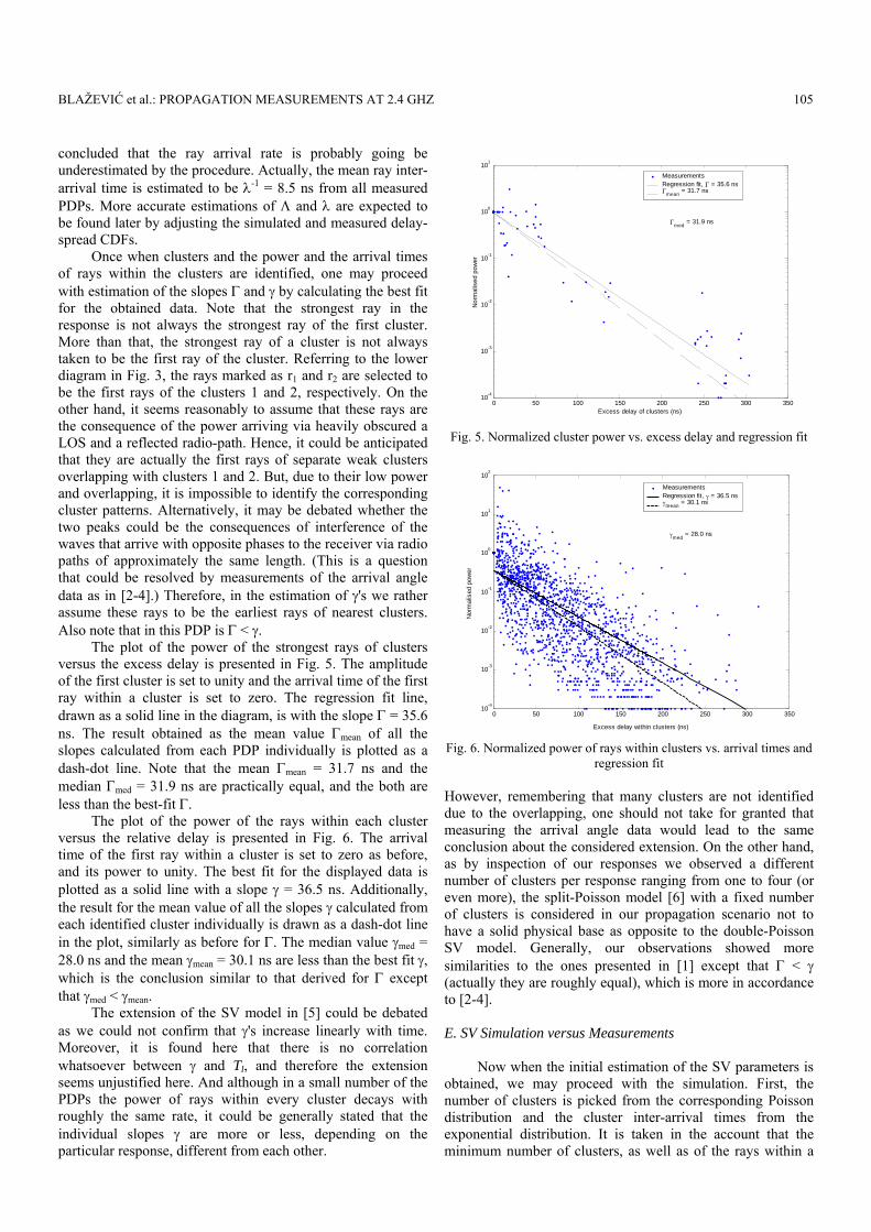
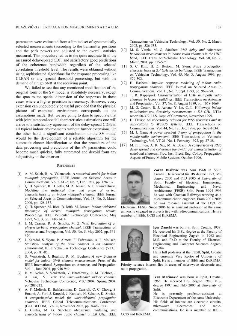
concluded that the ray arrival rate is probably going be underestimated by the procedure. Actually, the mean ray inter-arrival time is estimated to be λ-1 = 8.5 ns from all measured PDPs. More accurate estimations of Λ and λ are expected to be found later by adjusting the simulated and measured delay-spread CDFs. Once when clusters and the power and the arrival times of rays within the clusters are identified, one may proceed with estimation of the slopes Γ and γ by calculating the best fit for the obtained data. Note that the strongest ray in the response is not always the strongest ray of the first cluster. More than that, the strongest ray of a cluster is not always taken to be the first ray of the cluster. Referring to the lower diagram in Fig. 3, the rays marked as r1 and r2 are selected to be the first rays of the clusters 1 and 2, respectively. On the other hand, it seems reasonably to assume that these rays are the consequence of the power arriving via heavily obscured a LOS and a reflected radio-path. Hence, it could be anticipated that they are actually the first rays of separate weak clusters overlapping with clusters 1 and 2. But, due to their low power and overlapping, it is impossible to identify the corresponding cluster patterns. Alternatively, it may be debated whether the two peaks could be the consequences of interference of the waves that arrive with opposite phases to the receiver via radio paths of approximately the same length. (This is a question that could be resolved by measurements of the arrival angle data as in [2-4].) Therefore, in the estimation of γ's we rather assume these rays to be the earliest rays of nearest clusters. Also note that in this PDP is Γ < γ. The plot of the power of the strongest rays of clusters versus the excess delay is presented in Fig. 5. The amplitude of the first cluster is set to unity and the arrival time of the first ray within a cluster is set to zero. The regression fit line, drawn as a solid line in the diagram, is with the slope Γ = 35.6 ns. The result obtained as the mean value Γmean of all the slopes calculated from each PDP individually is plotted as a dash-dot line. Note that the mean Γmean = 31.7 ns and the median Γmed = 31.9 ns are practically equal, and the both are less than the best-fit Γ. The plot of the power of the rays within each cluster versus the relative delay is presented in Fig. 6. The arrival time of the first ray within a cluster is set to zero as before, and its power to unity. The best fit for the displayed data is plotted as a solid line with a slope γ = 36.5 ns. Additionally, the result for the mean value of all the slopes γ calculated from each identified cluster individually is drawn as a dash-dot line in the plot, similarly as before for Γ. The median value γmed = 28.0 ns and the mean γmean = 30.1 ns are less than the best fit γ, which is the conclusion similar to that derived for Γ except that γmed < γmean. The extension of the SV model in [5] could be debated as we could not confirm that γ's increase linearly with time. Moreover, it is found here that there is no correlation whatsoever between γ and Tl, and therefore the extension seems unjustified here. And although in a small number of the PDPs the power of rays within every cluster decays with roughly the same rate, it could be generally stated that the individual slopes γ are more or less, depending on the particular response, different from each other.

0 50 100 150 200 250 300 35010-4

10-3

10-2

10-1

100

101

Excess delay of clusters (ns)

Nor

mal

ised

pow

er

MeasurementsRegression fit, Γ = 35.6 nsΓmean = 31.7 ns

Γmed = 31.9 ns

Fig. 5. Normalized cluster power vs. excess delay and regression fit

0 50 100 150 200 250 300 35010-4

10-3

10-2

10-1

100

101

102

Excess delay within clusters (ns)

Nor

mal

ised

pow

er

MeasurementsRegression fit, γ = 36.5 nsγmean = 30.1 ns

γmed = 28.0 ns

Fig. 6. Normalized power of rays within clusters vs. arrival times and

regression fit However, remembering that many clusters are not identified due to the overlapping, one should not take for granted that measuring the arrival angle data would lead to the same conclusion about the considered extension. On the other hand, as by inspection of our responses we observed a different number of clusters per response ranging from one to four (or even more), the split-Poisson model [6] with a fixed number of clusters is considered in our propagation scenario not to have a solid physical base as opposite to the double-Poisson SV model. Generally, our observations showed more similarities to the ones presented in [1] except that Γ < γ (actually they are roughly equal), which is more in accordance to [2-4]. E. SV Simulation versus Measurements Now when the initial estimation of the SV parameters is obtained, we may proceed with the simulation. First, the number of clusters is picked from the corresponding Poisson distribution and the cluster inter-arrival times from the exponential distribution. It is taken in the account that the minimum number of clusters, as well as of the rays within a


cluster is one. The arrival time of the first cluster in a simulated PDP is set to zero. The mean number of rays per cluster is determined as λ/Λ. Then the number of rays generated within each cluster and the ray arrival times relative to the corresponding cluster arrival time are selected to be new Poisson random numbers. The amplitudes of the rays are picked from the Rayleigh distribution with the mean estimated by (2), while the phases are picked from a uniform distribution on [0, 2π). (Note that the powers of rays are then exponentially distributed.) With this procedure a simulated PDP is formed. In order to verify the first estimation of the SV parameters, 5000 responses were generated by the simulation and the delay-spread CDF is calculated. By comparison to the measured delay-spread CDF, the simulated CDF is found to be of different median value, while the tails of the distributions are not matched badly. Then, by adjusting Λ-1 to be 130 ns we found a much closer match of the considered CDFs. The final (fine) adjustment is obtained upon, by decreasing λ-1 from 8.5 ns calculated to 7 ns. The result is presented in Fig. 7, and all the estimations of SV parameters are listed and compared to the results from [1] and [4] in tables 2 and 3.

TABLE 2. ESTIMATIONS OF THE SLOPES Slope Median Mean Fit SV [1] UWB [4] Γ (ns) 31.9 31.7 35.6 60 27.9 γ (ns) 28.0 30.1 36.5 20 84.1

TABLE 3. OBSERVATIONS OF CLUSTER AND RAY ARRIVAL RATES Rate Estimated Adjusted SV [1] UWB [4]

Λ-1 (ns) 108.7 130 300 45.5 λ-1 (ns) 8.5 7 5 2.3

Now, in order to make an assessment of the adjusted SV parameters we calculate the coherence bandwidth from the simulated responses. The received waveforms at the corresponding ray arrival times are reconstructed assuming a sinc impulse and alternatively a Gaussian impulse. Amplitude and phase of the impulse correspond to the generated Rayleigh random amplitude and the generated uniform random phase, respectively. The width of the impulse is selected to be the theoretical response resolution of the VNA, and with the time step that is equal to the display resolution. The interval of the impulse spans from zero to 400 ns (which is more than enough to cover our responses) regardless of its excess delay. Then, all impulses are summed to form a simulated band-limited PDP (without the thermal noise) and displayed on the PC screen in arbitrary scale for an overview. Just for a check, we calculated the delay-spread CDFs for each selected type of the impulse and compared them with the simulated CDF calculated previously, and found that there are virtually no discrepancies among them. Then, the band-limited autocorrelations of the PDPs are calculated, from which the coherence bandwidth CDF is estimated for various threshold levels C. By inspection of the results for the two types of impulses, no differences between the coherence bandwidth CDFs could be found. The simulated coherence bandwidth CDFs for the different threshold levels C (0.9, 1/√2, 0.5, 1/e) are plotted on the same plots in Fig. 8 with the measured ones and with the theoretical minimum coherence bandwidth CDFs calculated by (6).

10 15 20 25 30 35 40 45 500

0.1

0.2

0.3

0.4

0.5

0.6

0.7

0.8

0.9

1

Delay spread σ (ns)

Pro

babi

lity(σ

< a

bsci

sa)

Empirical CDF

MeasurementsSimulation

Fig. 7. Measured delay-spread CDF vs. delay-spread CDF obtained

by SV simulation after adjusting Λ and λ

0 2 4 6 8 100

0.2

0.4

0.6

0.8

1

Coherence bandwidth BC (MHz)

Pro

babi

lity(

BC <

abs

cisa

)C = 0.9

Measured CDFTheoretical limit CDFSimulated CDF


0 10 20 30 40 500

0.2

0.4

0.6

0.8

1


Pro

babi

lity(

BC <

abs

cisa

)

C = 1/sqrt(2)


0 25 50 75 100 1250

0.2

0.4

0.6

0.8

1


Pro

babi

lity(

BC <

abs

cisa

)

C = 0.5


0 50 100 1500

0.2

0.4

0.6

0.8

1


Pro

babi

lity(

BC <

abs

cisa

)

C = 1/e


Fig. 8. Simulated coherence bandwidth CDF vs. measured CDF and

minimum theoretical bound CDF for different thresholds C Regardless of the threshold, the simulated CDFs are always positioned somewhere in between the two. The estimations of low coherence bandwidths are only slightly conservative, which is coupled to significantly more pessimistic estimations of high coherence bandwidths. However, as the simulation does not produce the solutions more optimistic than measurements, the moderately conservative estimations could be regarded as insurance that the operating radio channel will not be over-capacitated at any time. Nonetheless, regardless of the conclusion derived in [16] about a small influence to the coherence bandwidth of shape of the response compared to the standard deviation, it would be very interesting to explore whether the more sophisticated measurements and evaluation depicted in [2-4] could produce the different solutions to the SV parameters that would provide better predictions of the coherence bandwidths together with the delay-spreads.

5. CONCLUSIONS

In this paper we tried to apply the SV modeling procedure to the measurements in a university building. The


parameters were estimated from a limited set of systematically selected measurements (according to the transmitter positions and the peak power) and adjusted to the overall statistics measured. This procedure led us to the quite accurate fit to the measured delay-spread CDF, and satisfactory good predictions of the coherence bandwidth regardless of the selected correlation threshold level. The results were obtained without using sophisticated algorithms for the response processing like CLEAN or any special threshold processing, but with the demand of a high SNR at the receiving point. We failed to see that any mentioned modification of the original form of the SV model is absolutely necessary, except the span to the spatial dimension of the responses in those cases where a higher precision is necessary. However, every extension can undoubtedly be useful provided that the physical picture of examined environment corresponds to the assumptions made. But, we are going to dare to speculate that with joint temporal-spatial characteristics estimations one will arrive to a satisfactory agreement of the delay-spread CDFs in all typical indoor environments without further extensions. On the other hand, a significant contribution to the SV model would be the development of a reliable algorithm for the automatic cluster identification so that the procedure of the data processing and predictions of the SV parameters could become much quicker, fully automated and devoid from any subjectivity of the observer.

REFERENCES

[1] A. M. Saleh, R. A. Valenzuela: A statistical model for indoor

multipath propagation, IEEE Journal on Selected Areas in Communications, Vol. SAC-5, No. 2, Feb. 1987, pp. 128-137.

[2] Q. H. Spencer, B. D. Jeffs, M. A. Jensen, A. L. Swindlehurst: Modeling the statistical time and angle of arrival characteristics of an indoor multipath channel, IEEE Journal on Selected Areas in Communications, Vol. 18, No. 3, March 2000, pp. 128-137.

[3] Q. H. Spencer, M. Rice, B. Jeffs, M. Jensen: Indoor wideband time/angle of arrival multipath propagation results, Proceedings IEEE Vehicular Technology Conference, May 1997, Vol. 3, pp. 1410-1414.

[4] J. M. Cramer, R. A. Scholtz, M. Z. Win: Evaluation of an ultra-wide-band propagation channel, IEEE Transactions on Antennas and Propagation, Vol. 50, No. 5, May 2002, pp. 561-570.

[5] J. Karedal, S. Wyne, P. Almers, F. Tufvesson, A. F. Molisch: Statistical analysis of the UWB channel in an industrial environment, IEEE Vehicular Technology Conference (VTC), 2004, pp. 81-85.

[6] S. Venkatesh, J. Ibrahim, R. M. Buehrer: A new 2-cluster model for indoor UWB channel measurements, Proc. of the IEEE International Symposium on Antennas and Propagation, Vol. 1, June 2004, pp. 946-949.

[7] B. M. Nolan, S. Venkatesh, V. Bharadway, R. M. Buehrer, J. A. Tsai, V. Tech: The ultra-wideband indoor channel, Vehicular Technology Conference, VTC 2004, Spring 2004, pp. 208-212.

[8] A. F. Molisch, K. Balakrishnan, D. Cassioli, C. C. Chong, S. Emami, A. Fort, J. Karedal, J. Kunisch, H. Schantz, K. Siwiak: A comprehensive model for ultrawideband propagation channels, IEEE Global Telecommunications Conference (GLOBECOM), Vol. 6, November 2005, pp. 3648-3653.

[9] I. Cuiñas, M. G. Sánchez: Measuring, modeling, and characterizing of indoor radio channel at 5.8 GHz, IEEE

Transactions on Vehicular Technology, Vol. 50, No. 2, March 2002, pp. 526-535.

[10] M. S. Varela, M. G. Sánchez: RMS delay and coherence bandwidth measurements in indoor radio channels in the UHF band, IEEE Trans. on Vehicular Technology, Vol. 50, No. 2, March 2001, pp. 515-525.

[11] S. C. Kim, H. L. Bertoni, M. Stern: Pulse propagation characteristics at 2.4 GHz inside buildings, IEEE Transactions on Vehicular Technology, Vol. 45, No. 3, August 1996, pp. 579-592.

[12] H. Hashemi: Impulse response modeling of indoor radio propagation channels, IEEE Journal on Selected Areas in Communications, Vol. 11, No. 7, Sept. 1993, pp. 967-978.

[13] T. R. Rappaport: Characterization of UHF multipath radio channels in factory buildings, IEEE Transactions on Antennas and Propagation, Vol. 37, No. 8, August 1989, pp. 1058-1069.

[14] M. G. Cotton, R. J. Achatz, Y. Lo, C. L. Holloway: Indoor polarization and directivity measurements at 5.8 GHz, NTIA report 00-372, U.S. Dept. of Commerce, November 1999.

[15] H. Fleury: An uncertainty relation for WSS processes and its applications to WSSUS systems, IEEE Transactions on Communications, Vol. 44, No. 12, Dec. 1996, pp. 1632-1634.

[16] M. J. Gans: A power spectral theory of propagation in the mobile-radio environment, IEEE Transactions on Vehicular Technology, Vol. VT-21, No. 1, February 1972, pp. 27-38.

[17] M. P. Fitton, A. R. Nix, M. A. Beach: A comparison of RMS delay spread and coherence bandwidth for characterization of wideband channels, Proc. Inst. Elect. Eng. Colloq. Propagation Aspects of Future Mobile Systems, October 1996.

Zoran Blažević was born 1968 in Split, Croatia. He received his BS degree 1993, MS degree 2000 and PhD 2005 at University of Split, Faculty of Electrical Engineering, Mechanical Engineering and Naval Architecture (FESB) Split. From 1994-1996 he was with Croatian Railways working as a telecommunication engineer. From 2001-2006 he was research assistant at the Dept. of

Electronic, FESB. Since 2006 he is assistant professor at the same university engaged in projects tied with radiocommunications. He is a member of IEEE, CCIS and KoREMA.

Igor Zanchi was born in Split, Croatia, 1938. He received his B.Sc. degree at the Faculty of Electrical Engineering Zagreb in 1962 and M.S. and Ph.D at the Faculty of Electrical Engineering and Computer Sciences Zagreb, Croatia. He is full professor at the FESB, Split, Croatia and currently Vice Rector of University of Split. He is a member of IEEE and KoREMA.

Priority science interest lies in areas of microwave electronic and radio propagation.

Ivan Marinović was born in Split, Croatia, 1966. He received B.S. degree 1989, M.S. degree 1997 and PhD 2005 at University of Split. He is presently professor-assistant at Electronic Department of the same University. His fields of interest are electronic circuits, microwave electronics and radio-communications. He is a member of IEEE,

CCIS and KoREMA.


propagation measurements at 2.4 ghz inside a university

Documents