proost: object oriented approach to multiphase reactive
TRANSCRIPT
1
PROOST: Object oriented approach to multiphase reactive transport 1
modeling in porous media. 2
P. Gamazoa, L.J. Slootenb,e, J. Carrerab,e, M.W. Saaltinkc,e, S. Bead and J. Solera 3
a Departamento del Agua, CENUR LINO, Universidad de la República, Gral. Rivera 1350, 50000 Salto, Uruguay, 4
[email protected], [email protected] 5
b Institute of Environmental Assessment and Water Research (IDAEA), CSIC, c/Lluis Solè Sabarìs, s/n, 08028 Barcelona, Spain, 6
[email protected], [email protected] 7
c Dept. Geotechnical Engineering and Geosciences, Universitat Politecnica de Catalunya, UPC, c/Jordi Girona 1‐3, 08034 Barcelona, 8
Spain, [email protected] 9
d CONICET‐IHLLA República de Italia 780, 7300, Azul, Buenos Aires, Argentina, [email protected] 10
e Associated Unit: Hydrogeology Group (UPC‐CSIC) 11
12
Abstract 13
Reactive transport modelling involves solving several nonlinear coupled phenomena, among 14
them, the flow of fluid phases, the transport of chemical species and energy, and chemical 15
reactions.. There are different ways to account this coupling that might be more or less 16
suitable depending on the nature of the problem to be solved. In this paper we acknowledge 17
the importance of flexibility on reactive transport codes and how object oriented programming 18
can facilitate this feature. We present PROOST, an object oriented code that allows solving 19
reactive transport problems considering different coupling approaches. The code main classes 20
and their interactions are presented. PROOST performance is illustrated by the resolution of a 21
multiphase reactive transport problem where geochemistry affects hydrodynamic processes. 22
23
1. Introduction 24
Reactive transport models are tools that help to understand the hydraulic and chemical 25
behavior of natural and artificial porous media. It has been used to solve a broad range of 26
2
problems like groundwater remediation (Loomer et al. 2010), nuclear waste disposal 27
(MacQuarrie and Mayer 2005) and CO2 sequestration (Zhang et al. 2012) among others, from 28
micro scale (Trebotich et al. 2014) to field scale problems (Sassen et al. 2012). 29
Modeling reactive transport in porous media involves simulating several coupled phenomena: 30
phase flow, solute transport, and reactions. It may also involve multiphase flow, heat transport 31
and porous media deformation (Steefel et al. 2014,). These phenomena may be complex to 32
model individually, and modeling together brings on new difficulties associated with coupled 33
effects (Lichtner 1996). Which coupled effects have to be considered and the optimal solution 34
strategy for the coupled equations depend on the nature of the problem to be solved and may 35
vary significantly from case to case (Zhang et al. 2012). 36
The ideal reactive transport code would have to use an accurate, robust and efficient 37
numerical approach. However, it is difficult to obtain these goals with a single numerical 38
approach. Therefore, concessions have to be made and different coupling alternatives have to 39
be chosen at different levels. Numerical accuracy is generally preferred on other issues when 40
solving modeling research applications. On the other hand, when solving field scale problems, 41
efficiency and robustness have priority while accuracy remains within the bounds of the 42
uncertainty associated with model parameters (Yeh et al. 2012). 43
Two big family of methods were addressed to account for the coupling between solute 44
transport and chemical reaction processes: (1) the Operator Splitting (or Sequential Iterative 45
(or NON‐iterative) Approach, and (2) the Global Implicit or Direct Substitution Approach 46
(Saaltink et al. 2001). As regards the first one (i.e., the sequential methods), whether iterative 47
(SIA) or not (SNIA) adopt operator splitting techniques that effectively decouple component 48
transport equations. As regards the last one, direct substitution approaches (DSA) solve both 49
transport and chemical reactions simultaneously. A number of authors have studied the 50
numerical performance of these methods (Steefel and MacQuarrie, 1996), and they conclude 51
that in spite of the fact that the DSA is more accurate and robust, there are cases where the 52
3
SIA is more convenient from an efficiency‐accuracy point of view. In addition, SNIA may be 53
appropriated for scenario with Courant number smaller than 1 (Xu et al. 2012). Some reactive 54
transport codes are able to work with both of these approaches (CRUNCHFLOW, Steefel 2009; 55
DUMUX, Flemisch et al. 2011; HYDROGEOCHEM, Yeh et al, 2010; PFLOTRAN, Lichtner et al. 56
2013; RETRASOCODEBRIGHT et al. Saaltink et al. 2004.), while others use the fully implicit 57
approach (NUFT, Hao et al. 2012; MIN3P, Mayer et al. 2012), or different variants of operator 58
splitting techniques (CORE, Samper et al 2009; HYDRUS‐PHREEQC (HP1), Jacques et al. 2011; 59
HYTEC, Lagneau and Van Der Lee 2010; IPARS, Wheeler et al. 2012; OPENGEOSYS, Li et al. 2014; 60
ORCHESTRA, Meeussen 2003; PHAST, Parkhurst et al. 2010; PHREEQC, Parkhurst and Appelo 61
2013; PHT3D, Prommer and Post 2010; RT3D, Johnson and Truex 2006; STOMP, White and 62
McGrail 2005; TOUGHREACT, Xu et al. 2011). 63
On a more complex level is the coupling between phase conservation and reactive solute 64
transport. Most reactive transport codes decouple phase conservation (i.e. flow equation) 65
from reactive transport calculations (RT3D, MIN3P, PFLOTRAN , PHAST, RETRASOCODEBRIGHT, 66
HYTEC, TOUGHREACT). 67
This approach is convenient in most cases, but a numerically coupled solution will generally be 68
more suitable when the phenomena involved are highly physically coupled. One example of 69
this could be found in problems related with the CO2 sequestration in brine aquifers, which has 70
prompted the development of codes that solve coupled multiphase flow and reactive 71
transport (Fan et al. 2012) and even mechanical deformation (Zhang et al. 2012). Likewise, 72
Wissmeier and Barry (2008) showed that the consumption of water due to hydrated mineral 73
precipitation can have impacts on flow and solute transport for unsaturated flow problems. 74
These impacts can be even more important if gas transport is also considered because water 75
activity, which controls vapor pressure, is affected by capillary and osmotic effects. Moreover, 76
certain mineral paragenesis can fix water activity (producing an invariant point), causing the 77
geochemistry to control vapor pressure, which is the key variable for vapor flow (Risacher and 78
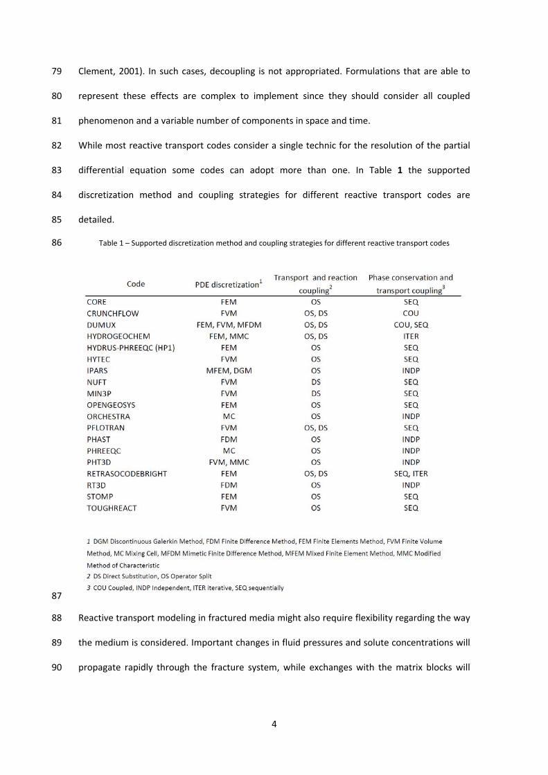
4
Clement, 2001). In such cases, decoupling is not appropriated. Formulations that are able to 79
represent these effects are complex to implement since they should consider all coupled 80
phenomenon and a variable number of components in space and time. 81
While most reactive transport codes consider a single technic for the resolution of the partial 82
differential equation some codes can adopt more than one. In Table 1 the supported 83
discretization method and coupling strategies for different reactive transport codes are 84
detailed. 85
Table 1 – Supported discretization method and coupling strategies for different reactive transport codes 86
87
Reactive transport modeling in fractured media might also require flexibility regarding the way 88
the medium is considered. Important changes in fluid pressures and solute concentrations will 89
propagate rapidly through the fracture system, while exchanges with the matrix blocks will 90
5
occur slowly. To account this, some reactive transport codes have included Multiple 91
Interacting Continua modeling (TOUGHREACT, PFLOTRAN). 92
In short, for reactive transport modeling the adopted coupling techniques, the partial 93
differential equation discretization method and the way as the domain is considered, may be 94
problem dependent. Therefore, a reactive transport code should include several solution 95
approaches to be used in a broad range of problems. Moreover, in order to ensure its use for 96
present and future problems, it must have an extensible design. A number of authors have 97
pointed out that object oriented (OO) programming facilitates the implementation of these 98
features (Commend and Zimmermann 2001, Filho and Devloo 1991). 99
The scientific community has been adopting OO techniques for problem solving since the end 100
of the last century (Forde et al. 1990, Slooten et al. 2010, Wang and Kolditz 2007). But only in 101
the last decade have OO codes been developed for reactive transport modeling. Meysman et 102
al. (2003) developed an OO reactive transport code for a single fluid phase. Gandy and 103
Younger (2007) developed an OO multiphase reactive transport code for pyrite oxidation and 104
pollutant transport in tailing ponds. Shao et al. (2009) include reactive transport calculations 105
into a Thermo‐Hydro‐Mechanic OO framework adopting a sequential non iterative approach 106
(SNIA). Bea et al. (2009) developed an OO module capable of solving reactive transport for a 107
single phase considering the SNIA, SIA or DSA approach. However, all of these codes, and most 108
of the procedural reactive transport codes, have a predefined strategy for dealing with 109
coupling effects. Particularly, they do not allow for changing number and definitions of 110
chemical components when solving flow and reactive transport in a coupled way. 111
The objective of this paper is to present an OO structure for reactive transport that can 112
accommodate different level of physical and chemical processes coupling. The structure 113
presented here is capable to model from single‐phase SIA problems to fully coupled 114
multiphase reactive transport problems. In addition, the best of our knowledge, it is the first 115
OO tool capable to account the occurrence of invariant points (e.g., for reference see Risacher 116
6
and Clement) in a reactive transport problem. This is an extreme case where geochemical 117
processes significantly affect fluid flow and the number and definitions of chemical 118
components may vary significantly in space and time. This structure has been implemented in 119
PROOST which was programmed in FORTRAN 95 following the OO paradigm, and until now 120
could solve single phase reactive transport by the SIA method and a fully coupled multi‐phase 121
reactive transport by the DSA method. 122
123
2. Equations to solve 124
Reactive transport modeling implies establishing several conservation principles, like mass or 125
energy conservation, expressed as partial differential equations (PDE), and several constitutive 126
and thermodynamic laws (such as retention curve or mass actions laws) expressed as algebraic 127
equations (AE). Darcy’s law is used to represent momentum conservation. In this section we 128
present a generic conservation equation to represent conservation principles in reactive 129
transport problems. We consider in detail the species and component conservation and we 130
briefly present the constitutive and thermodynamic laws. 131
2.1. General conservation equation 132
Conservation of a physical entity can be expressed as 133
,
AF
t
j (1) 134
Where A is the amount of per unit volume of medium, , j is the flux of due to the 135
driving force (e.g. advection or diffusion), and F is a sink source term. Since time and spatial 136
derivatives are involved, conservation equations usually take the form of a partial differential 137
equation (PDE). 138
2.2. Species and component conservation equation 139
7
The conservation of a species i belonging to phase , which is a particular case of equation 140
(1) has the following expression: 141
, , , ,1 1
Ne Nk
i i j i j j i j ij j
c L c Se re Sk rk ft
(2) 142
Where is the volumetric content of phase , ,ic is the species i concentration in 143
phase,,j iSe is the stoichiometric coefficient of the equilibrium reaction j for the specie i , 144
jre is the reaction rate of the equilibrium reaction j , and Ne is the number of equilibrium 145
reactions.,j iSk ,
jrk and Nk are analogous to ,j iSe ,
jre and Ne but for kinetic reactions. if is 146
an external sink‐source term, and L is the linear transport operator for the mobile phase 147
involving advective and diffusive‐dispersive processes: 148
, , ,i i D iL c c q j (3) 149
Mobile phase fluxes q are calculated according to Darcy’s law: 150
p q K g (4) 151
where , p K and are the conductivity tensor, pressure and density of the phase 152
respectively. Diffusive‐dispersive fluxes ,D ij are calculated according to Fick’s law: 153
, , , diff dispD i i ic c j D D D (5) 154
where diffD and
dispD are the diffusion and dispersion tensor for phase respectively and is 155
the tortuosity. 156
Note that the general sink source term of equation (1) F involves several different terms in 157
equation (2): 158
, ,1 1
Ne Nk
j i j j i j ij j
F Se re Sk rk f
(6) 159
8
There is no explicit expression for the equilibrium reaction rates jre , their value has to be such 160
that the corresponding mass action law is satisfied. Therefore, jre values can be written as a 161
function of both transport and chemical processes (De Simoni et al. 2005). A common 162
approach to avoid dealing with these terms is to formulate the conservation of components as 163
a linear combination of species that remain unaffected by equilibrium reactions. As such, 164
equilibrium reactive rates disappear from the conservation equations of components (Steefel 165
and MacQuarrie 1996). However, components may involve species belonging to different 166
phases, therefore conservation equation for components have to be written: 167
, , , i ii i i u uu u L u k ft t
(7) 168
Where ,iu and ,iu are the i component concentration in mobile phases and immobile 169
phases respectively, and iuk is a linear combination of the kinetic terms that affect the 170
species composing the component. We consider as immobile phases minerals and fluid‐solid 171
interface, despite the fact an interphase is not a phase from a thermodynamic point of view. 172
Note that the component conservation equation (7) has the same structure as equation (2). 173
The main difference is that a component iu may be present in more than one phase, while a 174
species ic belongs to a single phase. There are several ways of defining components and 175
therefore some freedom in the choice of components. This has led to formulations that try 176
defining components that do not affect each other, such as those proposed by Molins et al. 177
(2004), Kräutle and Knabner (2005) and Hoffmann et al. (2010). Saaltink et al. (1998) 178
introduced a definition that eliminates species whose activities are known and constant. That 179
is the case of minerals, that are considered as pure phases, so that their activity equals unity. 180
Also, the activity of water can be assumed unity for the case of diluted solutions. Minerals, 181
often considered as constant activity species, might appear or disappear from portions of the 182
domain due to precipitation‐dissolution processes. Therefore, under equilibrium assumption, 183
9
the dimension of the component vector, the number of components, may be different at each 184
discrete point in space and vary in time. This increases the difficulty of solving equation (7) 185
since the matrix system to be solved has a dynamic size, which significantly affects the code. 186
Once all component conservation and geochemical equations have been solved, all species 187
concentrations are known. Equilibrium reaction rates jre are then calculated form species 188
conservation equation (2). If constant activity species have been eliminated from the 189
component definition, their concentration must also to be calculated from equation (2). 190
191
2.3. Constitutive and thermodynamic laws 192
The literature provides several models for density, viscosity and diffusion coefficients of mobile 193
phases. These parameters are usually expressed as an explicit function of phase composition, 194
pressure and temperature. Several models express saturation and relative permeability as an 195
explicit function of capillary pressure and surface tension. All these relations lead to a local 196
system of equations, which is valid at every point of the domain. 197
Thermodynamic relations also form part of this local system of equations. The most important 198
of these are the chemical equilibrium reactions, which may be expressed by means of mass 199
action laws, as often done in reactive transport. Also required are models for the calculation of 200
activity, such as Debye‐Hückel (1923), or Pitzer (1973) and expressions for kinetic rate laws 201
(such as Monod or Lasaga, Mayer et al. 2002). 202
Minor changes on the solid matrix, like porosity changes due to mineral dissolution‐203
precipitation or clogging, may also be expressed as algebraic equations (Soleimani et al. 2009). 204
More complex mechanical processes, like deformation or consolidation, involve momentum 205
conservation equation and have to be solved as a PDE (Villar et al. 2008). 206
Constitutive and thermodynamic relationships define a set of algebraic equations (AE) that 207
have to be solved together with the conservation equations (PDE). 208
209
10
2.4. Numerical solution of the equations 210
Methods such as finite element or finite differences, among others, are normally used to 211
approximate time or space derivative terms in PDEs. Application of such methods leads to a set 212
of equations that represent the conservation principle for discrete portions of the domain 213
(representing nodes or cells). The current version of PROOST supports two methods: the Finite 214
Elements and the Mixed Finite Elements. Contrary to constitutive or thermodynamic laws, 215
these equations are not local, that is, equations at a discrete point are function of variables at 216
other discrete points. As constitutive and thermodynamic models (AEs) involve variables that 217
appear in the PDE, both AEs and PDEs may have to be solved simultaneously. Generally, the 218
resulting set of equations is non‐linear, which makes their solution more difficult. As 219
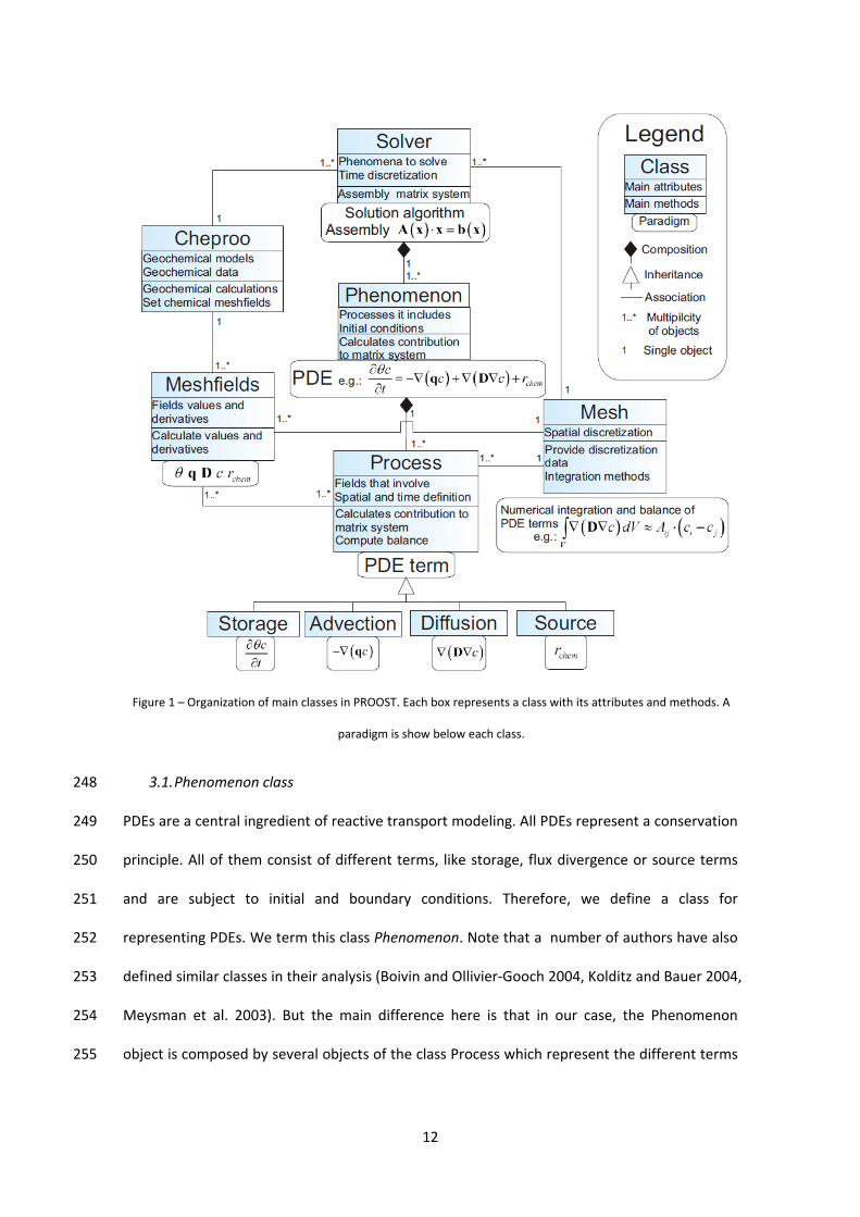
mentioned in the introduction different approaches can be adopted for solving these coupled 220
sets of equation: independently, sequentially, iteratively or coupled. 221
222
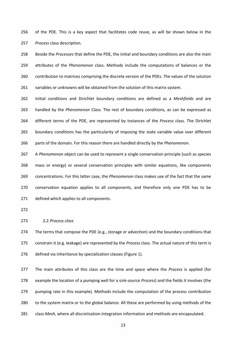
3. OO analysis of reactive transport modeling and PROOST class organization 223
According to the OO philosophy, the numerical solution of reactive transport can be 224
represented by a group of interacting objects. These objects belong to classes which define 225
common types of data and functionality. According to Filho and Devloo (1991), defining 226
suitable classes is the first and perhaps the most important step in software design under OO. 227
Our analysis was based on the following abstraction: reactive transport modeling is considered 228
as a set of equations (PDEs and AEs), representing the conservation of chemical species, that 229
need to be solved in a certain domain. These equations involve several variables or fields (such 230
as concentrations, density or porosity) which are also defined over portions of the same 231
domain. The domain is discretized and fields are defined over the discretized space (nodes or 232
cells). Using discretization techniques (such as finite element or finite differences methods) 233
PDEs are converted into a set of algebraic equations which represent a discrete version of the 234
11
PDE. For each discretized time interval, this set of equations can simultaneously be solved with 235
the AE or using an operator splitting technique. 236
The above description points to a natural class structure for our problems. The PDEs share 237
attributes such as terms in the equation, state variables or domain definitions, and also share 238
functionalities such as computing the balance or the matrices for the discretized PDE. 239
Therefore, we find it natural to define a class, termed Phenomenon, to identify PDEs. In the 240
same fashion, we define Process as the class whose instances will be specific terms in the PDE 241
(e.g. advection, dispersion, etc.). The class Meshfields defines objects representing various 242
properties defined over space (and time). To deal the geochemical processes we use the class 243
CHEPROO (CHEmical PRocesses Object Oriented, Bea et al. 2009). All these objects produce the 244
terms for the (non‐linear) discretized PDEs, which are solved with the functions of the class 245
Solver. The class organization described above is shown in Figure 1 and its detailed description 246
is given below. 247
12
3.1. Phenomenon class 248
PDEs are a central ingredient of reactive transport modeling. All PDEs represent a conservation 249
principle. All of them consist of different terms, like storage, flux divergence or source terms 250
and are subject to initial and boundary conditions. Therefore, we define a class for 251
representing PDEs. We term this class Phenomenon. Note that a number of authors have also 252
defined similar classes in their analysis (Boivin and Ollivier‐Gooch 2004, Kolditz and Bauer 2004, 253
Meysman et al. 2003). But the main difference here is that in our case, the Phenomenon 254
object is composed by several objects of the class Process which represent the different terms 255
Figure 1 – Organization of main classes in PROOST. Each box represents a class with its attributes and methods. A
paradigm is show below each class.
13
of the PDE. This is a key aspect that facilitates code reuse, as will be shown below in the 256
Process class description. 257
Beside the Processes that define the PDE, the initial and boundary conditions are also the main 258
attributes of the Phenomenon class. Methods include the computations of balances or the 259
contribution to matrices comprising the discrete version of the PDEs. The values of the solution 260
variables or unknowns will be obtained from the solution of this matrix system. 261
Initial conditions and Dirichlet boundary conditions are defined as a Meshfields and are 262
handled by the Phenomenon Class. The rest of boundary conditions, as can be expressed as 263
different terms of the PDE, are represented by instances of the Process class. The Dirichlet 264
boundary conditions has the particularity of imposing the state variable value over different 265
parts of the domain. For this reason there are handled directly by the Phenomenon. 266
A Phenomenon object can be used to represent a single conservation principle (such as species 267
mass or energy) or several conservation principles with similar equations, like components 268
concentrations. For this latter case, the Phenomenon class makes use of the fact that the same 269
conservation equation applies to all components, and therefore only one PDE has to be 270
defined which applies to all components. 271
272
3.2. Process class 273
The terms that compose the PDE (e.g., storage or advection) and the boundary conditions that 274
constrain it (e.g. leakage) are represented by the Process class. The actual nature of this term is 275
defined via inheritance by specialization classes (Figure 1). 276
The main attributes of this class are the time and space where the Process is applied (for 277
example the location of a pumping well for a sink‐source Process) and the fields it involves (the 278
pumping rate in this example). Methods include the computation of the process contribution 279
to the system matrix or to the global balance. All these are performed by using methods of the 280
class Mesh, where all discretization‐integration information and methods are encapsulated. 281
14
The Processes objects are the terms that constitute the conservation equations. A 282
Phenomenon can be formulated by combining different Processes. This class facilitates the 283
extensibility of the code because only the new terms (new specialization of the class Process) 284
have to be programmed to extend the set of equations that can be solved. It also allows 285
reusing code, since the same type of Processes can be used for different conservation 286
equations. For example, a diffusive process for a mass conservation equation and an energy 287
conservation equation are a different instance of the same class. Another example is the 288
extension of the component conservation equation from single phase to multiphase (equation 289
(7)). For this case, all processes have to be replicate for each mobile phase. This can be easily 290
done by considering new instances of the same Process objects. 291
There are certain limitations regarding the kind of Processes that can be added to a 292
Phenomenon, and are related to the numerical method chosen for solving it. The nature of the 293
considered Process has to be supported by the numerical method. For example, in its current 294
implementation, advective terms cannot be considered when solving a PDE with the Mixed 295
Finite Element Method. 296
Most boundary conditions are represented with objects of the class Process. Imposed fluxes 297
and variable dependent fluxes are considered through a Sink‐Source objects, which are 298
specialization of the class Process. As mentioned before Dirichlet boundary conditions are 299
handled by the Phenomenon class. 300
301
3.3. Mesh class 302
There are different techniques to solve PDEs numerically. All these techniques share an 303
approach for discretizing the spatial domain (such as nodes, elements or cells) and methods to 304
integrate (or differentiate) the terms (Process) of a PDE (Phenomenon) to produce a matrix 305
system from which the discrete solution of the PDE can be obtained. 306

15
Thus, all the data and functionality regarding spatial discretization and the discretization‐307
integration methods for solving PDE (such as finite element or finite differences) define a class 308
that we term Mesh. A number of authors have defined similar classes in their analysis. 309
However, most of them separate the domain discretization from the integration methods in 310
different classes (Commend and Zimmermann 2001, Wang and Kolditz 2007). This integration 311
was made because, despite of the fact that both methods can share a mesh (elements and 312
nodes), the mesh topological data required might be different. For example, Mixed Finite 313
Elements and Finite Elements can both use the same mesh, but Mixed Finite Elements needs 314
extra information about edges for 2D problems or sides for 3D. Another difference between 315
these two methods is that while Finite Elements gives a continuum scalar field for the solution 316
over the mesh, Mixed Finite Elements gives a vector field. Therefore, some aspects of the 317
spatial discretization are related to the integration method, and that is why both are consider 318
in a single object in PROOST. 319
The main attributes of the Mesh class are the domain discretization information (such as nodes 320
or cell coordinates and connectivity between these discrete elements). Methods include 321
yielding information of space discretization (such as the number of discrete elements and their 322
geometrical information), integrating the different terms of the conservation equation 323
(Processes) over the domain, and evaluating spatial properties of variables such as gradients. 324
The Mesh class allows incorporating new discretization‐integration numerical methods by 325
adding new specializations of the class. Two specializations of the class Mesh are currently 326
implemented in PROOST: the Finite Elements and the Mixed Finite Elements. 327
328
3.4. Meshfield class 329
Another important element of reactive transport modeling is the AEs that represent 330
constitutive and thermodynamic laws. Constitutive laws express one field as a function of 331
others. Thus a class termed Meshfield is defined to represent the projection of different scalar, 332
16
vector or tensor fields (such as pressure, flux or conductivity) in the discrete domain. The main 333
attributes of this class are the values and derivatives of a field for the discrete entities (nodes, 334
elements or cells) and the parameters of the function or constitutive laws they represent. The 335
main methods of the class are to calculate its values and derivatives, and to interpolate its 336
values over any point of the domain. Among others, Meshfield is used to represent retention 337
curves, relative permeability curves and dispersion coefficients. 338
For example a flux Meshfield object defined as h q T , can calculate its values and its 339
derivatives to transmissivity T and head h fields. When a Meshfield represents one of the 340
solution variables of the problems, like head in the previous example, its values are set by the 341
solver class. 342
The Meshfield class facilitates code extension since new constitutive laws can be easily added 343
to the code by creating new specializations. 344
345
3.5. CHEPROO class 346
Geochemical calculations for the component concentrations and kinetic rate laws of equation 347
(4) are in fact constitutive laws. Hence, we treat them as a specialization of a Meshfield, which 348
we term Chemical Meshfield. Many geochemical variables affect the evolution of the system 349
but do not appear explicitly in any PDE (e.g. the activity of aqueous species). For this reason 350
and also because of the complexity of some geochemical calculations, all geochemical models 351
and computations are encapsulated into a single object of a class termed CHEPROO. Only the 352
chemical variables that appear in PDE (such as component concentration or density) are stored 353
in a Chemical Meshfield. 354
The CHEPROO class uses a module with the same name, with an internal class hierarchy 355
including classes like species, phase and reaction (Bea et al.2009). CHEPROO attributes include 356
the geochemical models, such as those for activity coefficients, density or kinetic rates laws, 357
and the chemical data associated to each discrete point of the problem, such as concentrations 358
17
or components definition. CHEPROO includes methods for calculating the values and 359
derivatives of chemical variables (like component concentration) with respect to the solution 360
variables of the PDE, and to dump them into Chemical Meshfield objects. 361
CHEPROO also controls the number of chemical components. For some formulations, like the 362
one of Saaltink et al. (1998), the number of components may change in time and space. Thus, 363
CHEPROO has to provide information about the components in order to establish the 364
dimension of the final matrix system to be solved. 365
3.6. Solver class 366
A coupling strategy (coupled or decoupled) needs to be chosen when solving several PDEs. A 367
solution technique for non‐linear systems (Newton‐Raphson or Picard) is also needed. An 368
object of the Solver class will be in charge of solving a number of PDEs with a chosen solution 369
strategy: 370
Independently, there are no crossed influences between Phenomena (for example changes 371
on porosity due to chemical changes are not considered when solving fluid phase 372
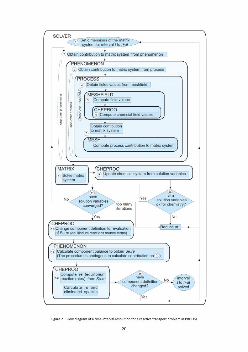
conservation) 373
Sequentially, influences between Phenomena are considered lagged in time (for the 374
porosity example, changes due to chemistry in time t are considered for flow in time t +dt) 375
Iteratively, all Phenomena are alternately solved until no significant changes on linking 376
variables occurs (for the porosity example, flow and transport are solved alternately until 377
no significant changes in porosity occurs) 378
Coupled, all Phenomena are solved at once. Solver attributes include the set of Phenomena, 379
the coupling strategy, the time discretization parameters or the convergence criteria. Methods 380
are required for assembling and solving the discretized PDE system, for time integration. To 381
address these, Solver uses other classes. For instances, matrix systems are handled by a class 382
termed Matrix that encapsulates matrix data and solution techniques for linear systems. 383
18
Solver is the class that contributes most to the flexibility of the code since it can be used to 384
solve several conservation equations following different strategies. For example, it might be 385
used to solve first a steady state phase conservation equation (for phase flow calculation) and 386
then a transient component conservation. Or it can be used to solve simultaneously the 387
component and energy conservation. 388
389
3.7. Component conservation Phenomenon for the SIA and DSA approach 390
Despite the fact that the SIA and DSA are two approaches for solving the same Phenomenon, 391
(the component conservation equation), the way this Phenomenon is formulated in PROOST 392
depends on the chosen approach. 393
When solving component conservation equations with the DSA approach the input 394
Phenomenon for PROOST should be the same as in equation (7). However, for the SIA 395
approach immobile species storage and kinetic reactions are treated as a sink‐source term : 396
,i iSIA i uf u kt
(8) 397
Thus the component conservation equation is written only in terms of mobile component 398
conservation: 399
, , i ii i SIA uu L u f ft
(9) 400
The Proost class organization allowed implementing the SIA method without many 401
modifications. The SIA sink source term was represented with the preexisting sink‐source 402
Process class. This process evaluates the values of the sink source term, which are given by a 403
Meshifield, and calculates its contribution to the discretized PDE system. By doing this, all the 404
19
complexity of this term is encapsulated in the class Cheproo, which sets the values of the SIA 405
source term in a Chemical Meshfield. 406
407
4. Solution procedure scheme for a time step 408
The interaction between PROOST objects can be illustrated by the solution of a time interval 409
for a reactive transport problem considering the DSA method. The flow diagram is shown in 410
Figure 2, from which 15 relevant points have been identified. 411
20
Figure 2 – Flow diagram of a time interval resolution for a reactive transport problem in PROOST
21
1. Solver establishes the size of the matrix system to be solved. This size depends on the 412
number of coupled phenomena and the dimension of each state variable. Recall that 413
component conservation dimension can be different for each discrete point and may 414
change among the iterative process. 415
2. Solver assembles the matrix system to be solved. To this end, Solver requests each 416
Phenomenon for its contribution. 417
3. Phenomenon requests for the contribution of all its Processes. 418
4. Each Proceses request the values of all the Meshfields to which it is related. 419
5. Meshfield computes its values. 420
6. CHEPROO calculates Chemical Meshfield values. 421
7. Mesh computes the contribution of the Process to the matrix system. 422
8. Matrix solves the matrix system. 423
9. Solver updates the calculated solution variables (concentrations, temperature or 424
pressures) in CHEPROO. 425
10. CHEPROO calculates the concentration of all species from these values (speciation). If 426
there are significant changes on chemical composition, like complete dissolution of 427
minerals in equilibrium or precipitation of new ones, geochemical calculation might not 428
converge. If that is the case, the length of time interval is reduced and the resolution 429
procedure is restarted. The user sets the ideal time step, but if the resolution of the matrix 430
system (which goes from step 2 to 11) exceeds a certain number of iterations, also set by 431
the user, the time step is reduced. 432
11. Solver controls the convergence of the PDEs linearization and resolution process. When 433
convergence is reached all variables involved in the phenomena are known, except 434
equilibrium reactions rates that were eliminated when solving component conservation 435
(equation (7)). These rates can be calculated from the species conservation equations 436
(equation (2)). In order to avoid the formality of formulating both components and species 437
22
Phenomenon, this is done by considering an alternative component definition; each mobile 438
species is considered a component. Therefore, the result of the balance of the new 439
component conservation will be the product of the stoichiometric coefficient and the 440
equilibrium reaction rates. These aspects are illustrated with an example in the next 441
section. 442
12. CHEPROO changes component definition (each mobile species is considered a component). 443
This step allows solving species conservation equations with the same structure used for 444
component conservation equations. This is one of the advantages of Proost class 445
organization. More details on this particular aspect will be given in section 6. 446
13. Phenomenon computes balance (similar to step 3). 447
14. CHEPROO calculates equilibrium reaction rates from Phenomenon balance. Some reactive 448
transport formulations, like the one of Saaltink et al. (1998), eliminate constant activity 449
species, like minerals, from component composition. These species concentration can be 450
calculated once the equilibrium reaction rates are known. 451
15. If the formulation considered eliminates constant activity species, the number of 452
component is affected by the disappearance or appearance of minerals. Therefore, 453
component definition has to be controlled after the eliminated species were calculated. If 454
component definition changes the resolution procedure has to be started for the new 455
definition, if not the resolution procedure for the time step is finished. 456
457
5. Code implementation 458
The code presented results from merging and expanding two existing codes: PROOST and 459
CHEPROO. The original design of PROOST was already capable of solving different 460
phenomenona, in a coupled or decoupled way, by considering different techniques for the 461
resolution of non‐linear system (such as Newton‐Raphson or Picard). However, such a design 462
only allowed solving Phenomenon objects that had one scalar field as unknown. Also 463
23
Phenomenon Processes had to be written explicitly as a function of the unknown variable. 464
These featured clashed with the resolution of component conservation, especially when the 465
DSA approach is considered. 466
The solution of component conservation equations involves considering the conservation 467
equation of several components. As the number of components and its definition might 468
change in time and space (because of complete dissolution or appearance of new mineral 469
species), the number of Phenomenon considered would also have to vary. In order to avoid 470
this difficulty, and as the same Processes affect all component concentrations, only one 471
Phenomenon is considered which applies to a vector variable: the component concentration 472
vector. Therefore, Phenomenon and Process classes were expanded to handle a vector variable 473
whose size may change in time and space. 474
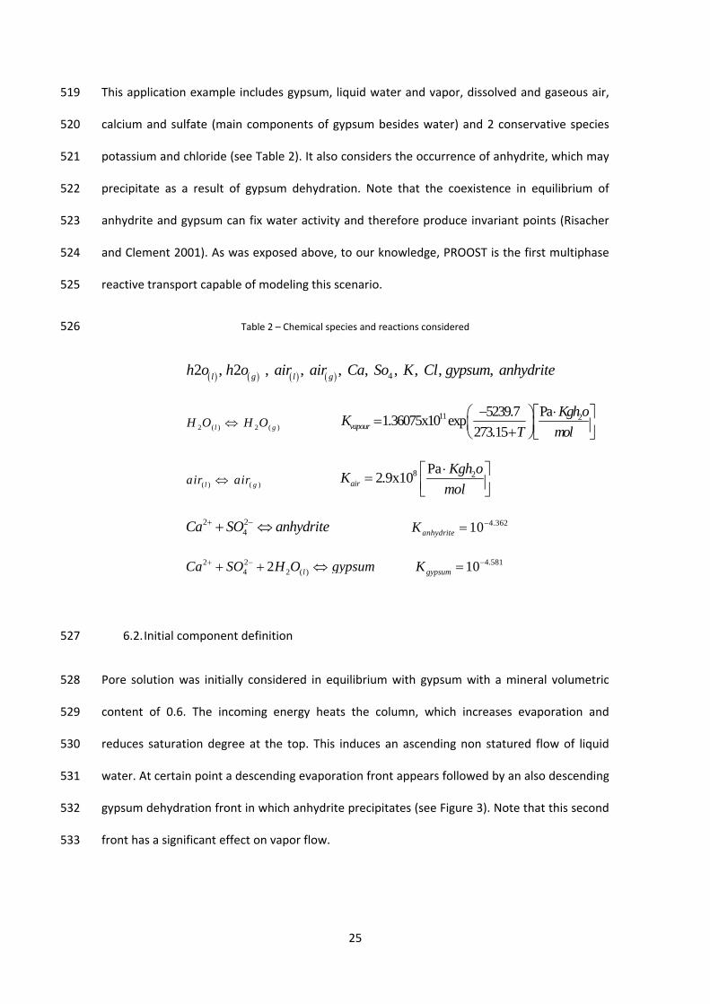
Processes where originally designed to represent terms of PDEs that directly involve the 475
unknowns of the problem (i.e. main state variables of the phenomenon: pressure for flow 476
equation, concentration for transport equation). For example, all Processes in a conservative 477
transport problem involve the solute concentration variable, which is also the unknown of this 478
problem. When solving reactive transport by the DSA method Processes are formulated in 479
terms of component concentrations, but the unknowns of the problem are the primary species 480
concentrations. Therefore, Phenomenon and Process classes were expanded so they can be 481
formulated in terms of any variable and not necessarily the unknown. 482
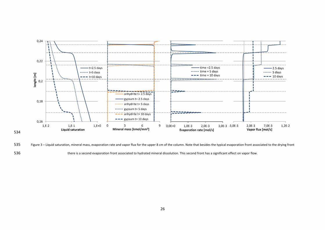
Originally, CHEPROO was capable of solving single phase reactive transport problems. 483
CHEPROO uses a matrix system calculated by another conservative transport code to 484
formulate and solve the reactive transport problem (Bea et al. 2008). In order to take 485
advantage of PROOST’s flexibility we choose to formulate and solve the multiphase reactive 486
transport equations in PROOST instead of CHEPROO. Therefore, CHEPROO was added to the 487
PROOST structure with the only purpose of performing the chemical calculations (speciation) 488
and provide geochemical variables values and derivatives. 489
24
Besides adding new services to make chemical variables available outside its module, several 490
improvements were made in CHEPROO. Phase properties like density, viscosity and enthalpy, 491
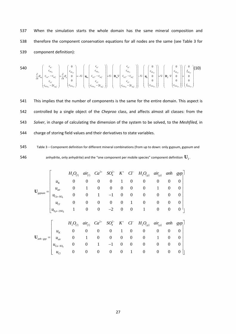
and capillary effect on water activity were added. The PROOST class organization allowed 492
representing all this chemical variables in the class Chemical meshfield. By doing this all the 493
work related to the evaluation, update and dependency of these fields to others (like pressure 494
or temperature) is done by pre existing methods. 495
Also a new speciation algorithm that uses the Newton‐Raphson method had to be 496
programmed in CHEPROO due to the high nonlinearity of concentrated solutions. CHEPROO 497
and PROOST were programmed in FORTRAN 95 following the OO paradigm. This language was 498
chosen for its high popularity among hydrogeologists and its excellent performance reputation. 499
Even though FORTRAN is not a full object‐oriented language it can directly support many of the 500
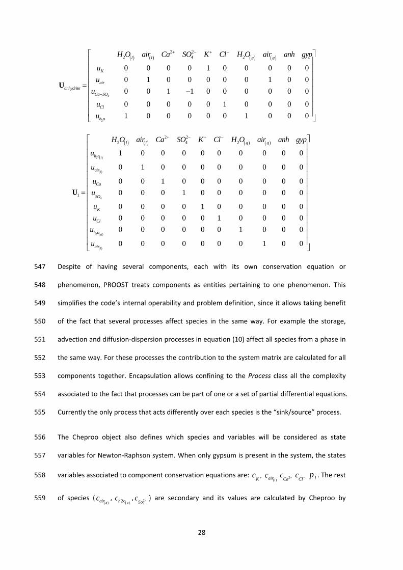
important concepts of OO programming. Details about OOP concepts in FORTRAN can be 501
found in Akin (1999), Carr (1999), Decyk et al. (1998), Gorelik (2004), Maley et al. (1996) and 502
Norton et al. (1998). 503
504
6. Application: 505
6.1. Application Description 506
In order to illustrate the classes introduced before, some aspects of the solution procedure 507
scheme for a time step (generically described in section 4) are shown for a concrete 508
application. We present the modeling of a 24 cm column of porous gypsum subjected to a 509
constant source of heat, in which a significant evaporation occurs. We will focus on the 510
component conservation equation. This synthetic example was designed for illustrating the 511
interaction between hydrodynamic and geochemical processes and it is described in detail by 512
Gamazo et al. (2012). Due to this interaction a compositional formulation was adopted and 513
therefore no phase conservation equations are explicitly solved. The finite element method 514
was used for the spatial discretization. One of the most interesting aspect of the application is 515
how the equilibrium reaction rates were calculated. This implies solving a different 516
conservation equation, species conservation instead of components. The PROOST structure 517
allowed to calculate the equilibrium reaction rates by using preexisting methods. 518
25
This application example includes gypsum, liquid water and vapor, dissolved and gaseous air, 519
calcium and sulfate (main components of gypsum besides water) and 2 conservative species 520
potassium and chloride (see Table 2). It also considers the occurrence of anhydrite, which may 521
precipitate as a result of gypsum dehydration. Note that the coexistence in equilibrium of 522
anhydrite and gypsum can fix water activity and therefore produce invariant points (Risacher 523
and Clement 2001). As was exposed above, to our knowledge, PROOST is the first multiphase 524
reactive transport capable of modeling this scenario. 525
Table 2 – Chemical species and reactions considered 526
42 , 2 , , , , , , , , l g l gh o h o air air Ca So K Cl gypsum anhydrite
2 ( ) 2 ( )l gH O H O
11 2Pa5239.71.36075x10 exp
273.15vapour
Kgh oK
T mol
( ) ( )l gair air 8 2Pa
2.9x10air
Kgh oK
mol
2 24Ca SO anhydrite 4.36210anhydriteK
2 24 2 ( )2 lCa SO H O gypsum 4.58110gypsumK
6.2. Initial component definition 527
Pore solution was initially considered in equilibrium with gypsum with a mineral volumetric 528
content of 0.6. The incoming energy heats the column, which increases evaporation and 529
reduces saturation degree at the top. This induces an ascending non statured flow of liquid 530
water. At certain point a descending evaporation front appears followed by an also descending 531
gypsum dehydration front in which anhydrite precipitates (see Figure 3). Note that this second 532
front has a significant effect on vapor flow. 533
26
534
Figure 3 – Liquid saturation, mineral mass, evaporation rate and vapor flux for the upper 8 cm of the column. Note that besides the typical evaporation front associated to the drying front 535
there is a second evaporation front associated to hydrated mineral dissolution. This second front has a significant effect on vapor flow. 536
27
When the simulation starts the whole domain has the same mineral composition and 537
therefore the component conservation equations for all nodes are the same (see Table 3 for 538
component definition): 539
2 2 2 2 24 4
2 24 4
22 2
0
0
0
2 2
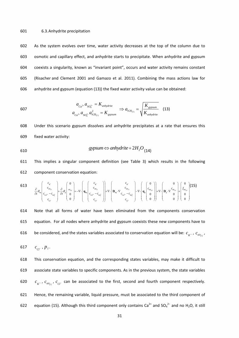
l l lg
gl l
K K K
air air airair
Ca So Ca So Caaq g aq aq
Cl Cl
h oh o h oSo So
c c c
c c cc
c c c c c ct t
c ccc c c c
q D
24
24
2 2 22
0 0 0
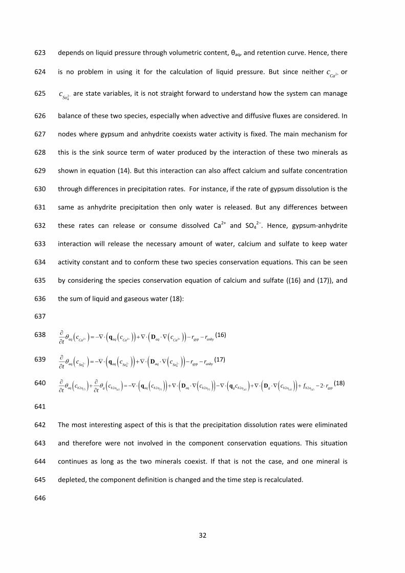
0 0 0
0 0 0
2
g g g
g g gl
air air air
So g g
Cl
h o h o h oh o So
c c f
cc c fc c
q D
(10) 540
This implies that the number of components is the same for the entire domain. This aspect is 541
controlled by a single object of the Cheproo class, and affects almost all classes: from the 542
Solver, in charge of calculating the dimension of the system to be solved, to the Meshfiled, in 543
charge of storing field values and their derivatives to state variables. 544
Table 3 – Component definition for different mineral combinations (from up to down: only gypsum, gypsum and 545
anhydrite, only anhydrite) and the “one component per mobile species” component definition 1U . 546
4
2 4
2 22 4 2
2
0 0 0 0 1 0 0 0 0 0
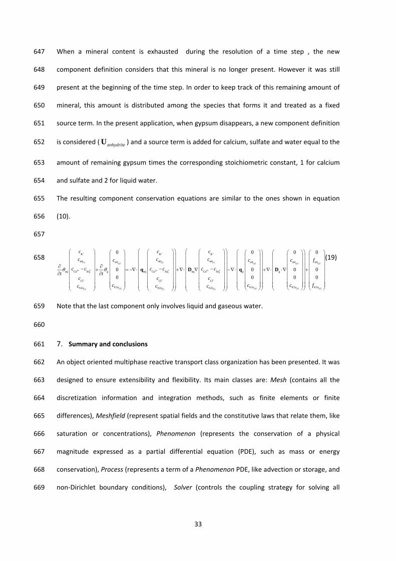
0 1 0 0 0 0 0 1 0 0
0 0 1 1 0 0 0 0 0 0
0 0 0 0 0 1 0 0 0 0
1 0 0 2 0 0 1 0 0 0
l l g g
K
airgypsum
Ca SO
Cl
h o SO
H O air Ca SO K Cl H O air anh gyp
u
u
u
u
u
U
4
2 22 4 2
0 0 0 0 1 0 0 0 0 0
0 1 0 0 0 0 0 1 0 0
0 0 1 1 0 0 0 0 0 0
0 0 0 0 0 1 0 0 0 0
l l g g
K
anh gyp air
Ca SO
Cl
H O air Ca SO K Cl H O air anh gyp
u
u
u
u
U
28
4
2
2 22 4 2
0 0 0 0 1 0 0 0 0 0
0 1 0 0 0 0 0 1 0 0
0 0 1 1 0 0 0 0 0 0
0 0 0 0 0 1 0 0 0 0
1 0 0 0 0 0 1 0 0 0
l l g g
K
airanhydrite
Ca SO
Cl
h o
H O air Ca SO K Cl H O air anh gyp
u
u
u
u
u
U
2
4
2
2 22 4 2
1
1 0 0 0 0 0 0 0 0 0
0 1 0 0 0 0 0 0 0 0
0 0 1 0 0 0 0 0 0 0
0 0 0 1 0 0 0 0 0 0
0 0 0 0 1 0 0 0 0 0
0 0 0 0 0 1 0 0 0 0
0 0 0 0 0 0 1 0 0 0
0 0 0 0 0 0 0 1 0 0
l
l
g
l
l l g g
h o
air
Ca
SO
K
Cl
h o
air
H O air Ca SO K Cl H O air anh gyp
u
u
u
u
u
u
u
u
U
Despite of having several components, each with its own conservation equation or 547
phenomenon, PROOST treats components as entities pertaining to one phenomenon. This 548
simplifies the code’s internal operability and problem definition, since it allows taking benefit 549
of the fact that several processes affect species in the same way. For example the storage, 550
advection and diffusion‐dispersion processes in equation (10) affect all species from a phase in 551
the same way. For these processes the contribution to the system matrix are calculated for all 552
components together. Encapsulation allows confining to the Process class all the complexity 553
associated to the fact that processes can be part of one or a set of partial differential equations. 554
Currently the only process that acts differently over each species is the “sink/source” process. 555
The Cheproo object also defines which species and variables will be considered as state 556
variables for Newton‐Raphson system. When only gypsum is present in the system, the states 557
variables associated to component conservation equations are: K
c lairc 2Ca
c Clc lp . The rest 558
of species ( gairc ,
2 gh oc , 24So
c ) are secondary and its values are calculated by Cheproo by 559
29
considering mass actions laws. Reaction rates and non‐mobile species concentrations are 560
calculated in a subsequent step. 561
In order to understand the physical meaning of component conservation equations, it is 562
helpful to associate state variables to specific components. For example, each of the species 563
chosen as state variables (K
c , lairc , 2Ca
c and Clc ) can be considered as the constituents of 564
the four first components of the conservation equations (10). The association of the liquid 565
pressure ( lp ) to a specific component is not straight forward. Liquid pressure is related to 566
liquid saturation which affects all components. Since the last component in equation (10) 567
contains all water species and only involves secondary species, liquid pressure can then be 568
associated to its main variable. However, variables like activity coefficients, density, viscosity, 569
gas pressure and liquid saturation, depend on all state variables and make the system fully 570
coupled. Nevertheless, the exercise of defining a main variable for every component provides 571
a more profound knowledge about variables dependency, which may be relevant for some 572
cases as will be shown in section 6.3. For that case water species is eliminated from the 573
component equation and both calcium and sulfate are defined as secondary variables. 574
As can be seen in Figure 2, matrix system assembling is the core of a time interval resolution. It 575
involves all the classes shown in Figure 1. 576
Once the system is solved there are still unknown variables to be calculated: the eliminated 577
species concentration and the equilibrium reaction rates. 578
These variables can be calculated by considering the species conservation equation. In order to 579
avoid formulating a different phenomenon the PROOST class organization allows using the 580
same structure as used for calculating component conservation for species conservation. This 581
is one of the advantages of the Proost class organization. The same phenomenon is considered 582
30
and only the component definition is changed. The new component definition considers every 583
mobile species as a component (see Table 3): 584
2 2
2 24 4
2 2
2
0
0
0 0
0
0
0
0
0 0
l l
g
l l
g
K K
air air
air
Ca Caaq g aq
So So
Cl Cl
h o h o
h o
c c
c c
c
c c
c ct t
c c
c cc
q
2
24
2
2 2
0 0
0 0
0
0 0
0 0
0 0
0 0
0
l
g g
l
g g
K
air
air air
Caaq g g
So
Cl
h o
h o h o
c
c
c c
c
c
c
cc c
D q D
2
2
0 0 0 00 1 0 0
1 0 0
0 0 0 1
0 0 0 1
0 0 0 0
0 0 1 2
0 1 0
g
g
air
air
h o
gyp
h o
fr
r
r
f
(11) 585
Note that all the processes in equation (11) are analogous to equation (10), except the last one. 586
This is the only term in equation (11) that has unknown variables ( airr , 2h or , gypsumr ), the other 587
terms involve known variables. In order to calculate these unknown variables the 1U 588
component definition is considered and a general method of the process class, balance, is used 589
to calculate all terms at the right hand side of equation (9): 590
2 2
24
2 2
2 2
000
0 0
0
0
0 0
2 0
0
l l
g
l
g
K K
air airair
airair
Ca Cagypaq g aq
So Sogyp
Cl
h o gyp h o
h o h o
c c
c crcr
c crc cr t t
cr r c
r c
q
2
2 24 4
2 2
2
0
0
0
0
0
0
0
0 0
l
g
l l
g
K
air
air
Caaq g
So
Cl Cl
h o h o
h o
c
c
c
c
c
c c
c cc
D q
2 2
0 0
0 0
0 0
0 0
0 0
0 0
g g
g g
air air
g
h o h o
c f
c f
D
591
(12) 592
The result is used by Cheproo to calculate the reaction rates (evaporation, volatilization of 593
dissolved air and gypsum precipitation). Note that the number of equations exceeds the 594
number of unknowns (eight and three, respectively). In theory, solution of all equations should 595
give the same reactions rates. For simplicity we used the least square method for the solution 596
of equation (9). Once the reaction rates are calculated, the mole variations of mineral species 597
can be computed (gypsum for this case). If a mineral is completely depleted or if the solution 598
has become saturated for a new mineral, components should be redefined and calculations for 599
the time step recalculated. 600
31
6.3. Anhydrite precipitation 601
As the system evolves over time, water activity decreases at the top of the column due to 602
osmotic and capillary effect, and anhydrite starts to precipitate. When anhydrite and gypsum 603
coexists a singularity, known as “invariant point”, occurs and water activity remains constant 604
(Risacher and Clement 2001 and Gamazo et al. 2011). Combining the mass actions law for 605
anhydrite and gypsum (equation (13)) the fixed water activity value can be obtained: 606
2 24
( )2 2
( )4
20220 l
l
anhydriteCa SO gypsumh
h gypsum anhydriteCa SO
a a K Ka
a a a K K
(13) 607
Under this scenario gypsum dissolves and anhydrite precipitates at a rate that ensures this 608
fixed water activity: 609
22gypsum anhydrite H O (14) 610
This implies a singular component definition (see Table 3) which results in the following 611
component conservation equation: 612
2 2 2 2 2 24 4 4
0 0
0 0
0 0
l l lg g
K K K
air air airair air
aq g aq aq g
Ca So Ca So Ca So
Cl Cl Cl
c c c
c c c c
c c c c c ct t
c c c
q D q
0 0
0 0
0 0
g gair air
g
c f
D
(15) 613
Note that all forms of water have been eliminated from the components conservation 614
equation. For all nodes where anhydrite and gypsum coexists these new components have to 615
be considered, and the states variables associated to conservation equation will be: K
c , lairc , 616
Clc , lp . 617
This conservation equation, and the corresponding states variables, may make it difficult to 618
associate state variables to specific components. As in the previous system, the state variables 619
Kc ,
lairc , Cl
c can be associated to the first, second and fourth component respectively. 620
Hence, the remaining variable, liquid pressure, must be associated to the third component of 621
equation (15). Although this third component only contains Ca2+ and SO42− and no H2O, it still 622
32
depends on liquid pressure through volumetric content, θaq, and retention curve. Hence, there 623
is no problem in using it for the calculation of liquid pressure. But since neither 2Cac or 624
24So
c are state variables, it is not straight forward to understand how the system can manage 625
balance of these two species, especially when advective and diffusive fluxes are considered. In 626
nodes where gypsum and anhydrite coexists water activity is fixed. The main mechanism for 627
this is the sink source term of water produced by the interaction of these two minerals as 628
shown in equation (14). But this interaction can also affect calcium and sulfate concentration 629
through differences in precipitation rates. For instance, if the rate of gypsum dissolution is the 630
same as anhydrite precipitation then only water is released. But any differences between 631
these rates can release or consume dissolved Ca2+ and SO42−. Hence, gypsum‐anhydrite 632
interaction will release the necessary amount of water, calcium and sulfate to keep water 633
activity constant and to conform these two species conservation equations. This can be seen 634
by considering the species conservation equation of calcium and sulfate ((16) and (17)), and 635
the sum of liquid and gaseous water (18): 636
637
2 2 2aq aq aq gyp anhyCa Ca Cac c c r r
t
q D (16) 638
2 2 24 4 4
aq aq aq gyp anhySo So Soc c c r r
t
q D (17) 639
2 2 2 2 2 2 2 2l g l l g g gaq h o g h o aq h o aq h o g h o g h o h o gypc c c c c c f r
t t
q D q D (18) 640
641
The most interesting aspect of this is that the precipitation dissolution rates were eliminated 642
and therefore were not involved in the component conservation equations. This situation 643
continues as long as the two minerals coexist. If that is not the case, and one mineral is 644
depleted, the component definition is changed and the time step is recalculated. 645
646
33
When a mineral content is exhausted during the resolution of a time step , the new 647
component definition considers that this mineral is no longer present. However it was still 648
present at the beginning of the time step. In order to keep track of this remaining amount of 649
mineral, this amount is distributed among the species that forms it and treated as a fixed 650
source term. In the present application, when gypsum disappears, a new component definition 651
is considered ( anhydriteU ) and a source term is added for calcium, sulfate and water equal to the 652
amount of remaining gypsum times the corresponding stoichiometric constant, 1 for calcium 653
and sulfate and 2 for liquid water. 654
The resulting component conservation equations are similar to the ones shown in equation 655
(10). 656
657
2 2 2 2 2 24 4 4
22 2 2
0
0
0
l l lg
gl l l
K K K
air air airair
Ca So Ca So Ca Soaq g aq aq
Cl Cl Cl
h oh o h o h o
c c c
c c cc
c c c c c ct t
c c ccc c c
q D
2 2 2
0 0 0
0 0 0
0 0 0
g g g
g g g
air air air
g g
h o h o h o
c c f
c c f
q D
(19) 658
Note that the last component only involves liquid and gaseous water. 659
660
7. Summary and conclusions 661
An object oriented multiphase reactive transport class organization has been presented. It was 662
designed to ensure extensibility and flexibility. Its main classes are: Mesh (contains all the 663
discretization information and integration methods, such as finite elements or finite 664
differences), Meshfield (represent spatial fields and the constitutive laws that relate them, like 665
saturation or concentrations), Phenomenon (represents the conservation of a physical 666
magnitude expressed as a partial differential equation (PDE), such as mass or energy 667
conservation), Process (represents a term of a Phenomenon PDE, like advection or storage, and 668
non‐Dirichlet boundary conditions), Solver (controls the coupling strategy for solving all 669
34
Phenomena and assembles the matrix system to solve) and CHEPROO (encapsulates all 670
thermodynamic date and perform geochemical calculations). 671
The flexibility and extensibility of PROOST come from the following particularities of its design. 672
Several Phenomenon can be formulated by combining the available Process. In order to solve a 673
new kind of Phenomenon, only new Processes have to be programmed. The Solver class can be 674
set to solve all Phenomena independently, sequentially or coupled.. New constitutive laws can 675
be easily added to the code by creating new specialization of the Meshfield class, and new 676
numerical methods for discretization‐integration of PDE can be added by implementing new 677
specializations of the Mesh class. The main challenging task, for solving reactive transport 678
problems, was to implement the ability of using changing definitions of components. This 679
could be achieved by considering the components as entities pertaining to one Phenomenon. 680
The flexibility of the structure allowed the implementation of the SIA method by mainly 681
creating a new specialization of the Messfield class.The performance of PROOST is illustrated 682
by describing the solution procedure for a concrete application: the modeling of a column of 683
porous gypsum subjected to a constant source of heat. The problem involves important 684
interaction between hydrodynamic and geochemical processes like the occurrence of invariant 685
points. The flexibility of the structure is shown in the example. In this regard, it highlights the 686
fact that a single phenomenon object is considered for representing both component and 687
species conservation in two different steps of the resolution procedure. This allows the 688
calculation of the equilibrium reaction rates using pre existing methods. 689
690
References 691
Akin, J. E. Object oriented programming via Fortran 90. Engineering Computations, 16, 26–48, 692
1999. 693
694
35
Bea, S.A.,Carrera, J., Ayora, C., Batlle, F. and Saaltink, M.W. Cheproo: A fortran 90 object‐695
oriented module to solve chemical processes in earth science models. Computers & 696
Geosciences, 35(6):1098–1112, 2009. 697
698
Boivin, C. and Ollivier‐Gooch, C. A toolkit for numerical simulation of pdes. ii. solving generic 699
multiphysics problems. Computer Methods in Applied Mechanics and Engineering, 193(36‐700
38):3891–3918, September 2004. 701
702
Carr, M. Using Fortran90 and object‐oriented programming to accelerate code development, 703
IEEE Antennas and Propagation Magazine, 41, 85–90, 1999 704
705
Commend, S. and Zimmermann, T. Object‐oriented nonlinear finite element programming: a 706
pimer. Advances In Engineering Software, vol. 32, no. 8, pp. 611_628, Aug. 2001. 707
708
Clement, T., Sun, Y., Hooker, B. and Petersen J. .Modeling multispecies reactive transport in 709
ground water. Ground Water Monitoring & Remediation, 18(2):79–92, 1998. 710
711
De Simoni, M., Carrera, J., Sanchez‐Vila, X., and Guadagnini, A. A procedure for the solution of 712
multicomponent reactive transport problems. Water Resources Research, 41(11):W11410, 713
November 2005. 714
715
Debye, P., Hückel, E.,.Thetheory of electrolytes. I .Lowering of freezing point and related 716
phenomena. Physikalische Zeitschrift 24, 185–206, 1923 717
718
Decyk, V. K., Norton, C. D. and Szymanski, B. K. How to support inheritance and run‐time 719
polymorphism in Fortran90, Computer Physics Communications, 115, 9–17, 1998. 720
36
721
Fan, Y., Durlofsky, L J. and Tchelepi H.A., A fully‐coupled flow‐reactive‐transport formulation 722
based on element conservation, with application to CO2 storage simulations, Advances in 723
Water Resources 42 47–61, 2012 724
725
Filho, J., Devloo, P. Object‐oriented programming in scientific computations: the beginning of a 726
new era. Engineering Computations, 8:81–87, 1991. 727
728
Flemisch, B., Darcis, M., Erbertseder, K., Faigle, B., Lauser, A., Mosthaf, K., Müthing, S., Nuske, 729
P., Tatomir, A., Wolff, M. and R. Helmig DuMux: DUNE for Multi‐{Phase, Component, Scale, 730
Physics, ...} Flow and Transport in Porous Media. Advances in Water Resources, 2011, 34(9): 731
1102‐1112. 732
733
Forde, B., Foschi, R.O., Stiemer, S.F. Object‐oriented finite element analysis. Computers and 734
Structures, 34(3):355–374, 1990. 735
736
Gamazo, P., Saaltink, M.W., Carrera, J., Slooten, L., Bea, S.A. A consistent compositional 737
formulation for multiphase reactive transport where chemistry affects hydrodynamics. Adv. 738
Water Resour. 35, 83–93, 2012. 739
740
Gandy, C. J. and Younger, P. L. An object‐oriented particle tracking code for pyrite oxidation 741
and pollutant transport in mine spoil heaps. Journal of Hydroinformatics, 9 (4):293–304, 2007. 742
743
Gorelik, A. M., Object‐oriented programming in modern Fortran. Programming and Computer 744
Software, 30, 173–179, 2004. 745
746
37
Hao, Y., Sun, Y., Nitao, J. J. Chapter 9: Overview of NUFT: A Versatile Numerical Model for 747
Simulating Flow. In: Zhang, F., Yeh, G.T., Parker, J.C. (eds.) Groundwater reactive transport 748
models Bentham e‐Books. Bentham Science Publishers, 2012. http://www.bentham.org 749
750
Hoffmann, J, S. Kräutle, P. Knabner, A parallel global‐implicit 2‐D solver for reactive transport 751
problems in porous media based on a reduction scheme and its application to the MoMaS 752
benchmark problem, Comput. Geosci., 14, 421‐433, doi: 10.1007/s10596‐009‐9173‐7, 2010. 753
754
Jacques, D., Šimůnek, J.,Mallants, D., van Genuchten, M.T., Yu, L.: A coupled reactive transport 755
model for contaminant leaching from cementitious waste matrices accounting for solid phase 756
alterations. In: Proceedings Sardinia 2011, Thirteenth International Waste Management and 757
Landfill Symposium, 2011. 758
759
Johnson, C.D. and Truex, M.J. RT3D Reaction Modules for Natural and Enhanced Attenuation 760
of Chloroethanes, Chloroethenes, Chloromethanes, and Daughter Products, PNNL‐15938 761
Pacific Northwest National Laboratory, Richland, Washington, 2006 762
763
Kolditz, O. and Bauer, S. A process‐oriented approach to computing multi‐field problems in 764
porous media. Journal of Hydroinformatics, 6:225–244, 2004. 765
766
Kräutle, S. and P. Knabner, A new numerical reduction scheme for fully coupled 767
multicomponent transport‐reaction problems in porous media, Water Resour. Res., 41, 768
W09414, doi:10.1029/2004WR003624, 2005. 769
38
770
Lagneau, V., Van Der Lee, J. HYTEC results of the MoMas reactive transport benchmark. 771
Computational Geosciences, Springer Verlag (Germany), 14, pp.435‐449, 2010. 772
773
Li, D., Bauer, S., Benisch, K., Graupner, B. and Beyer, C., OpenGeoSys‐ChemApp: a coupled 774
simulator for reactive transport in multiphase systems and application to CO2 storage 775
formation in Northern Germany, Acta Geotechnica, 9:67–79, 2014 776
777
Lichtner, P.C. Continuum formulation of multicomponent–multiphase reactive transport in: 778
Lichtner, P.C., Steefel, C.I., Oelkers, E.H. (Eds.), Reactive Transport in Porous Media, Reviews in 779
Mineralogy, vol. 34, pp. 1 –81, 1996. 780
781
Lichtner, P.C., Hammond, G.E., Lu, C., Karra, S., Bisht, G., Andre, B., Mills, R.T., Kumar, J.: 782
PFLOTRAN User manual: A Massively Parallel Reactive Flow and Transport Model for 783
Describing Surface and Subsurface Processes, 2013 784
785
Loomer, D.B., Al, T.A., Banks, V..J, Parker, B.L., Mayer, K.U. Manganese valence in oxides 786
formed from in situ chemical oxidation of TCE by KMnO4, Environmental Science & Technology 787
Aug 1; 44(15):5934‐9, 2010 788
789
MacQuarrie, K., Mayer K. U. Reactive transport modeling in fractured rock: A state‐of‐the‐790
science review, Earth‐Science Reviews, Vol. 72 Issue 3/4, p189‐227. 39p., 2005 791
792
Maley, D., Kilpatrick, P. L., Schreiner, E. W., Scott, N. S. and Diercksen, G. H. F. The formal 793
specification of abstract data types and their implementation in fortran 90: Implementation 794
39
issues concerning the use of pointers. Computer Physics Communications, vol. 98, no. 1‐2, pp. 795
167‐180, Oct. 1996 796
797
Mayer, K. U.; Frind, E. O. & Blowes, D. W. Multicomponent reactive 798
transport modeling in variably saturated porous media using a generalized 799
formulation for kinetically controlled reactions Water Resources Research, 800
38, 1174, 2002 801
802
Mayer, K. U., Amos, R. T., Molins, S. and Gérard F. Chapter 8: Reactive Transport Modeling in 803
Variably Saturated Media with MIN3P: Basic Model Formulation and Model Enhancements. In: 804
Zhang, F., Yeh, G.T., Parker, J.C. (eds.) Groundwater reactive transport models Bentham e‐805
Books. Bentham Science Publishers, 2012. http://www.bentham.org 806
807
Meeussen, J.C.: ORCHESTRA: An object‐oriented framework for implementing chemical 808
equilibrium models, Environmental Science & Technology, 37, 1175–1182, 2003. 809
810
Meysman, F.J. R., Middelburg, J. J., Herman, P. M. J. and Heip, C. H. R. Reactive transport in 811
surface sediments. i. model complexity and software quality. Computers & Geosciences, 812
29(3):291–300, April 2003. 813
814
Molins, S., Carrera, J., Ayora, C. and Saaltink, M.W. A formulation for decoupling components 815
in reactive transport problems. Water Resour. Res., 40(10):W10301–, October 2004. 816
817
Norton, C. D., Decyk, V. and Slottow, J. Applying fortran 90 and object‐oriented techniques to 818
scientific applications. Object‐Oriented Technology, vol. 1543, pp. 462‐463, 1998 819
820
40
Parkhurst, D.L., Appelo, C.A.J.: Description of input and examples for PHREEQC version 3—a 821
computer program for speciation, batch‐reaction, one‐dimensional transport, and inverse 822
geochemical calculations, U.S. Geological Survey Techniques and Methods, book 6, chap. A43, 823
2013 824
825
Pitzer, S. Thermodynamics of electrolytes. I. Theoretical basis and general equations. Journal of 826
Physical Chemistry 77 (2), 268–277, 1973 827
828
Prommer, H., Post, V..: PHT3D, A Reactive Multicomponent Transport Model for Saturated 829
Porous Media. User’s Manual v2.10, 2010. 830
831
Risacher, F. and Clement, A. A computer program for the simulation of evaporation of natural 832
waters to high concentration. Computers & Geosciences, 27(2):191–201, March 2001. 833
834
Saaltink, M. W., Ayora, C., and Carrera, J. A mathematical formulation for reactive transport 835
that eliminates mineral concentrations. Water Resources Research, 34(7):1649–1656, July 836
1998. 837
838
Saaltink, M. W., Carrera, J. and Ayora, C. On the behavior of approaches to simulate reactive 839
transport. Journal of Contaminant Hydrology, 48(3‐4):213–235, April 2001. 840
841
Saaltink, M. W., Batlle, F., Ayora, C., Carrera, J., and Olivella, S. Retraso, a code for modeling 842
reactive transport in saturated and unsaturated porous media. Geologicaacta, 2, Nº3:235–251, 843
2004. 844
845
41
Samper, J., Xu, T., Yang, C. , A sequential partly iterative approach for multicomponent reactive 846
transport with CORE2D, Computational Geosciences, Volume 13, Issue 3, pp 301‐316, 2009 847
848
Sassen, D. S., S. S.Hubbard, S. A.Bea, J.Chen, N.Spycher, and M. E.Denham, Reactive facies: An 849
approach for parameterizing field‐scale reactive transport models using geophysical methods, 850
Water Recourses Research., 48, W10526, 2012 851
852
Shao, H., Dmytrieva, S. V., Kolditz, O., Kulik, D. A., Pfingsten, W. and Kosakowski, G. Modeling 853
reactive transport in non‐ideal aqueous‐solid solution system. Applied Geochemistry, 854
24(7):1287–1300, July 2009 855
856
Slooten, L.J., Batlle, F. , and Carrera, J. An XML based Problem Solving Environment for 857
Hydrological Problems. XVIII Conference on Computational Methods in Water Resources 858
(CMWR) http://congress.cimne.com/cmwr2010, 2010. 859
860
Soleimani, S., Van Geel, P.J., Isgor, O. B., Mostafa, M. B. Modeling of biological clogging in 861
unsaturated porous media. Journal of Contaminant Hydrology. Volume 106, Issues 1–2, 15 862
Pages 39–50, 2009. 863
864
Steefel, C. I. and MacQuarrie, K.T.B. Approaches to modeling of reactive transport in porous 865
media. Reviews in Mineralogy and Geochemistry (Reactive Transport in Porous Media) January 866
1996; v. 34;1; p. 85‐129, 34:85–129, 1996. 867
868
Steefel, C. I., CrunchFlow Software for Modeling Multicomponent Reactive Flow and Transport 869
User’s guide, Earth Sciences Division Lawrence Berkeley National Laboratory 2009. 870
871
42
Steefel, C. I., Appelo, C. A. J., Arora, B., Jacques, D., Kalbacher, T., Kolditz, O., Lagneau, V., 872
Lichtner, P. C., Mayer, K. U., Meeussen, J. C. L., Molins, S., Moulton, D., Shao, H., Šimůnek, J., 873
Spycher, N., Yabusaki, S. B., Yeh, G. T. Reactive transport codes for subsurface environmental 874
simulation. Computational Geosciences, 1‐34, 2014 875
876
Trebotich, D., Adams, M.F., Molins, S., Steefel, C.I., Shen, C., High‐Resolution Simulation of 877
Pore‐Scale Reactive Transport Processes Associated with Carbon Sequestration, Computing in 878
Science & Engineering, vol.16, no. 6, pp. 22‐31, Nov.‐Dec. 2014 879
880
Villar, M.V., Sánchez, M., Gens, A. Behaviour of a bentonite barrier in the laboratory: 881
Experimental results up to 8 years and numerical simulation. Physics and Chemistry of the 882
Earth, Parts A/B/C , Volume 33, Supplement 1, Pages S476–S485, 2008. 883
884
Wang, W. and Kolditz, O.Object‐oriented finite element analysis of thermo‐hydro‐mechanical 885
(THM) problems in porous mediaInt. J. Numer. Meth. Engng; 69:162‐201, 2007 886
887
White, M. D. and McGrail, B. P., STOMP Subsurface Transport Over Multiple Phases, PNNL‐888
15482, Pacific Northwest National Laboratory, Richland, Washington, 2005 889
890
Wheeler, M.F., Sun, S., and Thomas, S.G., Chapter 2 'Modeling of flow and reactive transport in 891
IPARS'. In: Zhang, F., Yeh, G.T., Parker, J.C. (eds.) Groundwater reactive transport models 892
Bentham e‐Books. Bentham Science Publishers, 2012. http://www.bentham.org 893
894
Wissmeier, L. and Barry, D.A. Reactive transport in unsaturated soil: Comprehensive modelling 895
of the dynamic spatial and temporal mass balance of water and chemical components. 896
Advances in Water Resources, 31(5):858–875, 2008. 897
43
898
Yeh, G.T., Fang, Y.L., Zhang, F., Sun, J.T., Li, Y., Li, M.H., Siegel, M.D.: Numerical modeling of 899
coupled fluid flow and thermal and reactive biogeochemical transport in porous and fractured 900
media. Computational Geoscience 14, 149–170, 2010. 901
902
Yeh, G.T., Tripathi, V.J., Gwo, J.P., Cheng, H.P., Cheng, R.J., Salvage, K.M., Li, M.H., Fang, Y.L., Li, 903
Y., Sun, J.T., Zhang, F., Siegel, M.D.: Chapter 1: HYDROGEOCGEM: A coupled model of variably 904
saturated flow, thermal transport, and reactive biogeochemical transport.. In: Zhang, F., Yeh, 905
G.T., Parker, J.C. (eds.) Groundwater reactive transport models Bentham e‐Books. Bentham 906
Science Publishers, 2012. http://www.bentham.org 907
908
Xu, T., Spycher, N., Sonnenthal, E., Zhang, G., Zheng, L., Pruess, K.: TOUGHREACT Version 2.0: A 909
simulator for subsurface reactive transport under non‐isothermal multiphase flow conditions. 910
Computers & Geosciences, 37, 763–774, 2011. 911
912
Xu, T., Spycher, N., Sonnenthal, Spycher, G., E., Zhang, G., Zheng, L., Pruess, K. Chapter 3 913
TOUGHREACT: A simulator for subsurface reactive transport under non‐isothermal multiphase 914
flow conditions. In: Zhang, F., Yeh, G.T., Parker, J.C. (eds.) Groundwater reactive transport 915
models Bentham e‐Books. Bentham Science Publishers, 2012. http://www.bentham.org 916
917
Zhang, R.,Yin X., Winterfeld, P.H. and Wu Y. A fully coupled Model of nonisothermal 918
multiphase flow, geomechanics and chemistry during CO2 sequestration in brine aquifers, 919
Proceedings, TOUGH Symposium 2012, Lawrence Berkeley National Laboratory, Berkeley, 920
California, September 17‐19, 2012 921