proof of the kurlberg-rudnick rate...
TRANSCRIPT

Annals of Mathematics 174 (2011), 1–54doi: 10.4007/annals.2011.174.1.1
Proof of the Kurlberg-Rudnickrate conjecture
By Shamgar Gurevich and Ronny Hadani
To our teacher Joseph Bernstein on the occasion of his 60th birthday
Abstract
In this paper we present a proof of the Hecke quantum unique ergodicity
rate conjecture for the Hannay-Berry model of quantum mechanics on the
two-dimensional torus. This conjecture was stated in Z. Rudnick’s lectures
at MSRI, Berkeley 1999, and ECM, Barcelona 2000.
0. Introduction
0.1. The Hannay-Berry model. In the paper “Quantization of linear maps
on the torus-Fresnel diffraction by a periodic grating”, published in 1980 [17],
the physicists J. Hannay and Sir M. V. Berry explore a model for quantum
mechanics on the two-dimensional symplectic torus (T, ω). Hannay and Berry
suggested quantizing simultaneously the functions on the torus and the linear
symplectic group Γ = SL2(Z).
0.2. Quantum chaos. One of their main motivations was to study the
phenomenon of quantum chaos [3], [4], [33], [34] in this model. More precisely,
they considered an ergodic discrete dynamical system on the torus, which is
generated by a hyperbolic automorphism A ∈ SL2(Z). Quantizing the system,
we replace: the classical phase space (T, ω) by a finite-dimensional Hilbert
spaceH~, classical observables, i.e., functions f ∈ C∞(T), by operators π~(f) ∈End(H~), and classical symmetries by a unitary representation ρ~ : SL2(Z) −→U(H~). A fundamental meta-question in the area of quantum chaos is to
understand the ergodic properties of the quantum system ρ~(A), at least in
the semi-classical limit as ~→ 0.
0.3. Schnirelman’s theorem. Analogous with the case of the Schrodinger
equation, consider the following eigenstate problem:
(0.3.1) ρ~(A)ϕ = λϕ, ϕ ∈ H~.
A fundamental result, valid for a wide class of quantum systems which are as-
sociated to ergodic classical dynamics, is Schnirelman’s theorem [35], asserting
1

2 SHAMGAR GUREVICH and RONNY HADANI
that in the semi-classical limit “almost all” eigenstates becomes equidistributed
in an appropriate sense. A variant of Schnirelman’s theorem also holds in our
situation [5]. More precisely, in the semi-classical limit ~ → 0, for “almost
all” eigenstates ϕ of the operator ρ~(A), the corresponding Wigner distribu-
tion 〈ϕ|π~(·)ϕ〉 : C∞(T) −→ C approaches the phase space average∫T · |ω|. In
this respect, it seems natural to ask whether there exist exceptional sequences
of eigenstates? Namely, eigenstates that do not obey the Schnirelman’s rule
(“scarred” eigenstates). It was predicted by Berry [3], [4], that the “scar-
ring” phenomenon is not expected to be seen for quantum systems associated
with “generic” chaotic classical dynamics. However, in our situation the dy-
namical system is not generic, and exceptional eigenstates were constructed.
Indeed, it was confirmed mathematically in [11], that certain ρ~(A)-eigenstates
might localize. For example, in that paper, a sequence of eigenstates ϕ was
constructed, for which the corresponding Wigner distribution approaches the
measure 12 δ0 + 1
2 |ω| on T.
0.4. Hecke quantum unique ergodicity. A quantum system that obeys
Schnirelman’s rule is also called quantum ergodic. Can one impose some nat-
ural conditions on the eigenstates (0.3.1) so that no exceptional eigenstates
will appear? Namely, Quantum Unique Ergodicity will hold. This question
was addressed in a paper by Kurlberg and Rudnick [25]. In this paper they
formulated a rigorous notion of Hecke quantum unique ergodicity for the case
~ = 1p . The following is a brief description of that work. The basic observation
is that the degeneracies of the operator ρ~(A) are coupled with the existence
of symmetries. There exists a commutative group of operators that commutes
with ρ~(A). In more detail, the representation ρ~ factors through the quotient
group Γp w SL2(Fp). We denote by TA ⊂ Γp the centralizer of the element
A, now considered as an element of the quotient group Γp. The group TA is
called (cf. [25]) the Hecke torus corresponding to the element A. The Hecke
torus acts semisimply on H~. Therefore, we have a decomposition
H~ =⊕
χ:TA−→C∗Hχ,
where Hχ is the Hecke eigenspace corresponding to the character χ. Con-
sider a unit eigenstate ϕ ∈ Hχ and the corresponding Wigner distribution
Wχ : C∞(T) −→ C, defined by the formula Wχ(f) = 〈ϕ|π~(f)ϕ〉. The main
statement in [25] proves an explicit bound of the semi-classical asymptotic of
Wχ(f) ∣∣∣∣Wχ(f)−∫Tf |ω|
∣∣∣∣ ≤ Cfp1/4
,

PROOF OF THE KURLBERG-RUDNICK RATE CONJECTURE 3
where Cf is a constant that depends only on the function f . In Rudnick’s
lectures at MSRI, Berkeley 1999 [32], and ECM, Barcelona 2000 [33], he con-
jectured that a stronger bound should hold true; that is,
Conjecture 0.1 (Rate Conjecture). The following bound holds :∣∣∣∣Wχ(f)−∫Tf |ω|
∣∣∣∣ ≤ Cfp1/2
.
The basic clues suggesting the validity of this stronger bound come from
two main sources. The first source is computer simulations [24] accomplished
over the years to give extremely precise bounds for considerably large values
of p. A more mathematical argument is based on the fact that for special
values of p, in which the Hecke torus splits, namely, TA ' F∗p, one is able to
compute explicitly the eigenstate ϕ ∈ Hχ and as a consequence to give an
explicit formula for the Wigner distribution [26], [6]. More precisely, in case
ξ ∈ Tee, i.e., a character, the distribution Wχ(ξ) turns out to be equal to the
exponential sum1
p
∑a∈F∗p
ψ
Åa+ 1
a− 1
ãσ(a)χ(a),
where σ denotes the Legendre character, and ψ is a nontrivial additive char-
acter of Fp. This sum is very similar to the Kloosterman sum and the classical
Weil bound [36] yields the result.
In this paper a proof for the rate conjecture is presented, treating both
cases of split and inert (nonsplit) tori in a uniform manner. A fundamental
idea in our approach concerns a nontrivial relation between two seemingly
different dynamical systems. One which is attached to a split (“noncompact”)
torus and the other which is attached to a nonsplit (“compact”) torus. This
relation is geometric in nature and can be formally described in the framework
of algebraic geometry.
0.5. The geometric approach. The basic observation to be made is that
the theory of quantum mechanics on the torus, in case ~ = 1p , can be equiva-
lently recast in the language of representation theory of finite groups in char-
acteristic p. We will endeavor to give a more precise explanation of this mat-
ter. Consider the quotient Fp-vector space V = Tee/pTee, where Tee is the
lattice of characters on T. We denote by H = H(V) the Heisenberg group.
The group Γp w SL2(Fp) is naturally identified with the group of linear sym-
plectomorphisms of V. We have an action of SL2(Fp) on H. The Stone-von
Neumann theorem states that there exists a unique irreducible representation
π : H −→ GL(H), with the nontrivial central character ψ, for which its isomor-
phism class is fixed by SL2(Fp). This is equivalent to saying that H is equipped
with a compatible projective representation ρ : SL2(Fp) −→ PGL(H). Noting

4 SHAMGAR GUREVICH and RONNY HADANI
that H and SL2(Fp) are the sets of rational points of corresponding algebraic
groups, it is natural to ask whether there exist an algebro-geometric object
that underlies the pair (π, ρ). The answer to this question is positive. The
construction is proposed in an unpublished letter of Deligne to Kazhdan [10].
Briefly, the content of this letter is a construction of Representation Sheaves
Kπ and Kρ on the algebraic varieties H and SL2 respectively. One obtains, as
a consequence, the following general principle:
(∗) Motivic Principle. All quantum mechanical quantities in the Hannay-
Berry model are motivic in nature.
By this we mean that every quantum-mechanical quantity Q, is associated
with a vector space VQ endowed with a Frobenius action Fr : VQ −→ VQ, so
that
Q = Tr(Fr|VQ).
The main contribution of this paper is to implement this principle. In partic-
ular, we show that there exists a two-dimensional vector space Vχ, endowed
with an action Fr : Vχ −→ Vχ, so that
Wχ(ξ) = Tr(Fr|Vχ ).
This, combined with a bound on the modulus of the eigenvalues of Frobenius,
i.e., ∣∣∣e.v(Fr|Vχ )∣∣∣ ≤ 1
p1/2,
completes the proof of the rate conjecture.
0.6. Remarks. There are several remarks that we would like to make at
this point
Remark 1: Discreteness principle. “Every” quantityQ that appears in the
Hannay-Berry model admits a discrete spectrum in the following arithmetic
sense: Q can take only values which are finite linear combinations of terms with
absolute value of the form pi/2 for i ∈ Z. This is a consequence of the motivic
principle (*) and Deligne’s weight theory [9]. This puts some restrictions on
the possible values of the modulus |Q|. We believe that this principle can
be effectively used in various situations in order to derive strong bounds out
of weaker bounds. A striking example would be a possible alternative trivial
“proof” for the bound |Wχ(ξ)| ≤ Cξp1/2
:
|Wχ(ξ)| ≤ Cξp1/4
⇒ |Wχ(ξ)| ≤ Cξp1/2
.
Kurlberg and Rudnick proved in their paper [25] the weaker bound |Wχ(ξ)| ≤Cξp1/4
. This strongly indicates that the stronger bound |Wχ(ξ)| ≤ Cξp1/2
is valid.

PROOF OF THE KURLBERG-RUDNICK RATE CONJECTURE 5
Remark 2: Higher dimensional exponential sums. The bound that we
prove, |Wχ(ξ)| ≤ 2+o(1)√p , for ξ 6= 0, implies the bound on the operator norm
‖AvTA(ξ)‖ ≤ 2+o(1)√p , where AvTA(ξ) = 1
|TA|∑
B∈TA
ρ~(B)π~(ξ)ρ~(B−1). This,
on the one hand, implies1 the bound
(0.6.1) |AvTA(ξ)|N ≤p1/N (2 + o(1))
√p
,
where |AvTA(ξ)|N = (Tr|AvTA(ξ)|N )1/N is the N -Schatten norm of AvTA(ξ).
On the other hand, one can compute explicitly
(0.6.2) |AvTA(ξ)|2N2N =p
|TA|2N∑
(x1,...,x2N )∈X
ψ
Ç∑i<j
ω(xi, xj)
å,
where X = (x1, . . . , x2N )| xi ∈ Oξ,∑xi = 0 and Oξ = TA · ξ ⊂ V denotes
the orbit of ξ under the action of TA. Combining (0.6.1) and (0.6.2) we obtain
a nontrivial bound for N ≥ 3 on the higher dimensional exponential sum
(0.6.3)∑
(x1,...,x2N )∈X
ψ
Ç∑i<j
ω(xi, xj)
å≤Ç|TA| · (2 + o(1))
√p
å2N
= O(pN ).
It would be interesting to know whether there exists an independent proof for
this bound and whether this representation theoretic approach can be used to
prove nontrivial bounds for other interesting higher dimensional exponential
sums.
0.7. Sato-Tate conjecture. The next level of the theory is to understand
the complete statistics of the Hecke-Wigner distributions for different Hecke
states. More precisely, let us fix a nonzero character ξ ∈ Tee. For every
nonquadratic character χ : TA −→ C∗ we consider the normalized value
Wχ(ξ) = |TA|√p Wχ(ξ), which lies in the interval [−2, 2] (see Theorem 4.2). Now,
running over all multiplicative characters we define the following atomic mea-
sure on the interval [−2, 2]:
µp =1
|TA|∑χ
δWχ(ξ).
One would like to describe the limit measure (if it exists!). This is the content
of another conjecture of Kurlberg and Rudnick [26]:
1For an operator O on a Hilbert space H, |O| = (O∗O)12 ; for a finite-dimensional space
|O|N ≤ (dimH)1N ||O||.

6 SHAMGAR GUREVICH and RONNY HADANI
Conjecture (analogue of the Sato-Tate conjecture). The following limit
exists :
limp→∞
µp = µST,
where µST is the push-forward of the normalized Haar measure on SU(2) to
the interval [−2, 2] through the map g 7→ Tr(g).
We hope that using the methodology described in this paper one will be
able to gain some progress in proving this conjecture.
Remark. Note that the family Wχ(ξ)χ∈T∨Aruns over a nonalgebraic
space of parameters. Hence, we do not know how to apply Deligne’s equidis-
tribution theory (cf. Weil II [9]) directly in order to solve the Sato-Tate Con-
jecture.
0.8. Results.
0.8.1. Kurlberg-Rudnick conjecture. The main result of this paper is The-
orem 3.1, which is the proof of the Kurlberg-Rudnick rate conjecture (Conjec-
ture 0.1) on the asymptotic behavior of the Hecke-Wigner distributions.
0.8.2. Weil representation. We introduce two new constructions of the
Weil representation over finite fields.
(a) The first construction is stated in Theorem 2.3 and is based on the
Rieffel quantum torus A~, for ~ = 1p . This approach is essentially equivalent to
the classical approach [13], [18], [23], [37] that uses the representation theory
of the Heisenberg group in characteristic p. The fundamental difference is that
the quantum torus is well defined for every value of the parameter ~.
(b) Canonical Hilbert space (Kazhdan’s question). The second construc-
tion uses the “method of Canonical Hilbert Space” (see Appendix A). This
approach is based on the following statement:
Proposition (Canonical Hilbert space). Let (V, ω) be a two-dimensional
symplectic vector space over the finite field Fq . There exists a canonical Hilbert
space HV attached to (V, ω).
An immediate consequence of this proposition is that all symmetries of
(V, ω) automatically act on HV. In particular, we obtain a linear representa-
tion of the group Sp = Sp(V, ω) on HV. This approach has higher dimensional
generalization, for the case where V is of dimension 2n. This generalization
will be published by the authors elsewhere.
Remark. Note the main difference of our construction from the classical
approach due to Weil (cf. [37]). The classical construction proceeds in two
stages. Firstly, one obtains a projective representation of Sp, and secondly,

PROOF OF THE KURLBERG-RUDNICK RATE CONJECTURE 7
using general arguments about the group Sp one proves the existence of a
linearization. A consequence of our approach is that there exists a distinguished
linear representation, and its existence is not related to any group theoretic
property of Sp. We would like to mention that this approach answers, in
the case of the two-dimensional Heisenberg group, a question of Kazhdan [21]
dealing with the existence of Canonical Hilbert Spaces for co-adjoint orbits
of general unipotent groups. The main motive behind our construction is the
notion of oriented Lagrangian subspace. This idea was suggested to us by
Bernstein [2].
0.8.3. Deligne’s Weil representation sheaf. We include for the sake of com-
pleteness (see Appendix A.4) a formal presentation of Deligne’s letter to Kazh-
dan [10] that places the Weil representation on a complete algebro-geometric
ground. As far as we know, the content of this letter was never published.
This construction plays a central role in the proof of the Kurlberg-Rudnick
conjecture.
0.9. Structure of the paper. The paper is naturally separated into four
parts:
Part I consists of Sections 1, 2 and 3. In Section 1 we discuss classical me-
chanics on the torus. In Section 2 we discuss quantum mechanics a la Hannay
and Berry, using the Rieffel quantum torus model. In Section 3 we formulate
the quantum unique ergodicity theorem, i.e., Theorem 3.1. This part of the
paper is self-contained and consists of mainly linear algebraic considerations.
Part II: Section 4. This is the main part of the paper, consisting of the
proof of the Kurlberg-Rudnick conjecture. The proof is given in two stages.
The first stage consists of mainly linear algebraic manipulations to obtain
a more transparent formulation of the statement, resulting in Theorem 4.2.
In the second stage we venture into algebraic geometry. All linear algebraic
constructions are replaced by sheaf theoretic objects, concluding with the Ge-
ometrization Theorem, i.e., Theorem 4.4. Next, the statement of Theorem 4.2
is reduced to a geometric statement, the Vanishing Lemma, i.e., Lemma 4.6.
The remainder of the section is devoted to the proof of Lemma 4.6. For the
convenience of the reader we include a large body of intuitive explanations for
all the constructions involved. In particular, we devote some space explain-
ing Grothendieck’s Sheaf-to-Function Correspondence procedure which is the
basic bridge connecting Parts I and II.
Part III: Appendix A. In Section A.1 we describe the method of canon-
ical Hilbert space. In Section A.2 we describe the Weil representation in this
manifestation. In Section A.3 we relate the invariant construction to the more
classical constructions, supplying explicit formulas that will be used later. In

8 SHAMGAR GUREVICH and RONNY HADANI
Section A.4 we give a formal presentation of Deligne’s letter to Kazhdan [10].
The main statement of this section is Theorem A.5, in which the Weil repre-
sentation sheaf K is introduced. We include in our presentation only the parts
of that letter which are most relevant to our needs. In particular, we consider
only the two-dimensional case of this letter. In Section A.5 we supply proofs
for all technical lemmas and propositions appearing in the previous sections of
the appendix.
Part IV: Appendix B. In this appendix we supply the proofs for all
statements appearing in Parts I and II. In particular, we give the proof of
Theorem 4.4 which essentially consists of taking the Trace of Deligne’s Weil
representation sheaf K.
Acknowledgments. It is a pleasure to thank our Ph.D. adviser J. Bern-
stein for his interest and guidance in this project. We appreciate the con-
tribution of P. Kurlberg and Z. Rudnick who discussed with us their papers
and explained their results. We thank P. Sarnak for his invitation to visit
the Courant Institute in September 2004 to discuss our work. We would like
to thank D. Kazhdan for sharing his thoughts about the possible existence of
canonical Hilbert spaces. We thank our friend D. Gaitsgory for the discussions
on `-adic cohomologies and Deligne’s letter. We thank Y. Flicker for helpful
remarks. We thank B. Lewis for the editorial work. We thank M. Baruch, the
Technion, and M. Teicher, the Emmy Noether institute, for all the support.
We would like to acknowledge the referee for very important remarks. Finally,
we would like to thank P. Deligne for allowing us to publish his ideas about
the geometrization of the Weil representation. S.G. was partially supported
by BSF grant #2004200.
1. The classical torus
Let (T, ω) be the two-dimensional symplectic torus. Together with its
linear symplectomorphisms Γ w SL2(Z) it serves as a simple model of classical
mechanics (a compact version of the phase space of the harmonic oscillator).
More precisely, let T = W/Λ where W is a two-dimensional real vector space,
i.e., W ' R2 and Λ is a rank two lattice in W, i.e., Λ ' Z2. We obtain the
symplectic form on T by taking a nondegenerate symplectic form on W:
ω : W ×W −→ R.
We require ω to be integral, namely, ω : Λ × Λ −→ Z and normalized, i.e.,
Vol(T) = 1.
Let Sp(W, ω) be the group of linear symplectomorphisms, i.e., Sp(W, ω) 'SL2(R). Consider the subgroup Γ ⊂ Sp(W, ω) of elements that preserve the

PROOF OF THE KURLBERG-RUDNICK RATE CONJECTURE 9
lattice Λ, i.e., Γ(Λ) ⊆ Λ. Then Γ ' SL2(Z). The subgroup Γ is the group of
linear symplectomorphisms of T.
We denote by Λ∗ ⊆W∗ the dual lattice Λ∗ = ξ ∈W∗| ξ(Λ) ⊂ Z. The
lattice Λ∗ is identified with the lattice of characters of T by the following map:
ξ ∈ Λ∗ 7−→ e2πi<ξ,·> ∈ Tee,
where Tee = Hom(T,C∗).
1.1. The classical mechanical system. We consider a very simple discrete
mechanical system. A hyperbolic element A ∈ Γ, i.e., |Tr(A)| > 2, generates
an ergodic discrete dynamical system. The Birkhoff Ergodic Theorem states
that
limN→∞
1
N
N∑k=1
f(Akx) =
∫Tf |ω|,
for every f ∈ S(T) and for almost every point x ∈ T. Here S(T) stands for
a good class of functions, for example, trigonometric polynomials or smooth
functions.
We fix a hyperbolic element A ∈ Γ for the remainder of the paper.
2. Quantization of the torus
Quantization is one of the big mysteries of modern mathematics; indeed
it is not at all clear what the precise structure is which underlies quantization
in general. Although physicists have been using quantization for almost a
century, for mathematicians the concept remains altogether unclear. Yet, in
specific cases, there are certain formal models for quantization that are well
justified mathematically. The case of the symplectic torus is one of these
cases. Before we employ the formal model, it is worthwhile to discuss the
general phenomenological principles of quantization which are surely common
for all models.
Let us start with a model of classical mechanics, namely, a symplectic
manifold, serving as a classical phase space. In our case this manifold is the
symplectic torus T. Principally, quantization is a protocol by which one asso-
ciates a quantum “phase” space H to the classical phase space T, where H is a
Hilbert space. In addition, the protocol gives a rule by which one associates to
every classical observable, namely a function f ∈ S(T), a quantum observable
Op(f) : H −→ H, an operator on the Hilbert space. This rule should send a
real function into a self-adjoint operator.
To be more precise, quantization should be considered not as a single
protocol, but as a one-parameter family of protocols, parametrized by ~, the
Planck constant. For every fixed value of the parameter ~ there is a protocol
which associates to T a Hilbert space H~ and for every function f ∈ S(T) an

10 SHAMGAR GUREVICH and RONNY HADANI
operator Op~(f) : H~ −→ H~. Again the association rule should send real
functions to self-adjoint operators.
Accepting the general principles of quantization, one searches for a formal
model by which to quantize, that is, a mathematical model which will manu-
facture a family of Hilbert spaces H~ and association rules S(T) End(H~).
In this work we employ a model of quantization called the Weyl quantization
model.
2.1. The Weyl quantization model. The Weyl quantization model works
as follows. Let A~ be a one-parameter deformation of the algebra A of trigono-
metric polynomials on the torus. This algebra is known in the literature as
the Rieffel torus [31]. The algebra A~ is constructed by taking the free uni-
tal associative algebra over C generated by the symbols s(ξ) | ξ ∈ Λ∗ and
quotienting out by the relations s(ξ)s(η) = eπi~ω(ξ,η)s(ξ + η) and s(0) = 1.
Here ω is the form on W∗ induced by the original form ω on W. We point
out two facts about the algebra A~. First, when substituting ~ = 0 one gets
the group algebra of Λ∗, which is exactly equal to the algebra of trigonometric
polynomials on the torus. Second, the algebra A~ contains as a standard basis
the lattice Λ∗:
s : Λ∗ −→ A~.
Therefore, one can identify the algebras A~ ' A as vector spaces, where every
function f ∈ A can be viewed as an element of A~.
For a fixed ~, a representation π~ : A~ −→ End(H~) serves as a quantiza-
tion protocol; that is, for every function f ∈ A one has
f ∈ A ' A~ 7−→ π~(f) ∈ End(H~).
An equivalent way of saying this is
f 7−→∑ξ∈Λ∗
aξπ~(ξ),
where f =∑ξ∈Λ∗
aξ · ξ is the Fourier expansion of f .
To summarize: every family of representations π~ : A~ −→ End(H~) gives
us a complete quantization protocol. Yet, a serious question now arises, namely
what representations to choose? Is there a correct choice of representations,
both mathematically, but also perhaps physically? A possible restriction on the
choice is to choose an irreducible representation. Nevertheless, some ambiguity
still remains because there are several irreducible classes for specific values of ~.
We present here a partial solution to this problem in the case where the
parameter ~ is restricted to take only rational values [15]. Even more partic-
ularly, we take ~ to be of the form ~ = 1p where p is an odd prime number.
Before any formal discussion one should recall that our classical object is the
symplectic torus T together with its linear symplectomorphisms Γ. We would

PROOF OF THE KURLBERG-RUDNICK RATE CONJECTURE 11
like to quantize not only the observables A, but also the symmetries Γ. Next,
we shall construct an equivariant quantization of T.
2.2. Equivariant Weyl quantization of the torus. Let ~ = 1p and con-
sider the additive character ψ : Fp −→ C∗, ψ(t) = e2πitp . We give here a
slightly different presentation of the algebra A~. Let A~ be the unital asso-
ciative C-algebra generated by the symbols s(ξ) | ξ ∈ Λ∗ and the relations
s(ξ)s(η) = ψ( 12 ω(ξ, η))s(ξ + η), s(0) = 1. Here we consider ω as a map
ω : Λ∗ × Λ∗ −→ Fp. The lattice Λ∗ serves as a standard basis for A~:
s : Λ∗ −→ A~.
The group Γ acts on the lattice Λ∗, therefore, it acts on A~. It is easy to see
that Γ acts on A~ by homomorphisms of algebras. For an element B ∈ Γ, we
denote by f 7−→ fB the action of B on an element f ∈ A~.
Remark 2.1. This presentation of the algebra A~ was discovered in [16].
The two defining relations differ by (−1)ω(ξ,η) = sign(ξ + η)sign(ξ)sign(η),
where sign(ξ) = 1 if ξ ∈ 2Λ∗, sign(ξ) = −1 if ξ /∈ 2Λ∗. One has a Γ-equivariant
isomorphism from the algebra defined by the first presentation to the algebra
defined by the second presentation, sending s(ξ) in the first to sign(ξ)s(ξ) in
the second.
An equivariant quantization of the torus is a pair
π~ : A~−→End(H~),
ρ~ : Γ−→PGL(H~),
where π~ is a representation of A~ and ρ~ is a projective representation of Γ.
These two should be compatible in the following manner:
(2.2.1) ρ~(B)π~(f)ρ~(B)−1 = π~(fB),
for every B ∈ Γ and f ∈ A~. Equation (2.2.1) is called the Egorov identity.
Let us suggest now a construction of an equivariant quantization of the
torus. Given a representation π : A~ −→ End(H) and an element B ∈ Γ, we
construct a new representation πB : A~ −→ End(H):
(2.2.2) πB(f) = π(fB).
This gives an action of Γ on the set Irr(A~) of classes of irreducible representa-
tions. The set Irr(A~) has a very regular structure as a principal homogeneous
space over T. Moreover, every irreducible representation of A~ is finite dimen-
sional and of dimension p. The following theorem plays a central role in the
construction.

12 SHAMGAR GUREVICH and RONNY HADANI
Theorem 2.2 (Canonical invariant representation [15]). Let ~ = 1p , where
p is a prime.2 There exists a unique (up to isomorphism) irreducible represen-
tation (π~ ,H~) of A~ for which its equivalence class is fixed by Γ.
Let (π~ ,H~) be a representative of the fixed irreducible equivalence class.
Then for every B ∈ Γ we have
(2.2.3) πB~ ' π~ .
This means that for every element B ∈ Γ there exists an operator ρ~(B) acting
on H~ which realizes the isomorphism (2.2.3). The collection ρ~(B) : B ∈ Γconstitutes a projective representation
(2.2.4) ρ~ : Γ −→ PGL(H~).
Equations (2.2.2) and (2.2.3) also imply the Egorov identity (2.2.1).
The group Γ ' SL2(Z) is almost a free group and it is finitely presented. A
brief analysis [15] shows that every projective representation of Γ can be lifted
(linearized) into a true representation. More precisely, it can be linearized in
12 different ways, where 12 is the number of characters of Γ. In particular, the
projective representation (2.2.4) can be linearized (not uniquely) into an honest
representation. The next theorem (to be proved in Appendix B) proposes the
existence of a canonical linearization. Let Γp w SL2(Fp) denote the quotient
group of Γ modulo p.
Theorem 2.3 (Canonical linearization). Let ~ = 1p , where p 6= 2, 3.
There exists a unique linearization
ρ~ : Γ −→ GL(H~),
characterized by the property that it factors through the quotient group Γp
Γ //
ρ~@
@@@@
@@@@
@@Γp
ρ~
GL(H~).
From now on ρ~ means the linearization of Theorem 2.3.
Summary. Theorem 2.2 confirms the existence of a unique invariant rep-
resentation of A~, for every ~ = 1p . This gives a canonical equivariant quan-
tization (π~ , ρ~ ,H~). Moreover, for p 6= 2, 3 by Theorem 2.3, the projective
2Theorem 2.2 holds more generally, i.e., for all Planck constants of the form ~ = M/N
where M,N are co-prime integers. However, in this paper we will not need to consider this
generality.

PROOF OF THE KURLBERG-RUDNICK RATE CONJECTURE 13
representation ρ~ can be linearized in a canonical way to give an honest rep-
resentation of Γ which factors through Γp.3 Altogether, this gives a pair
π~ : A~−→End(H~),
ρ~ : Γp−→GL(H~)
satisfying the following compatibility condition (Egorov identity)
ρ~(B)π~(f)ρ~(B)−1 = π~(fB),
for every B ∈ Γp, f ∈ A~. The notation π~(fB) means that we take any
pre-image B ∈ Γ of B ∈ Γp and act by it on f . Note, that the operator π~(f B)
does not depend on the choice of B. In the following, we denote the Weil
representation ρ~ by ρ~ and consider Γp to be the default domain.
2.3. The quantum mechanical system. Let (π~ , ρ~ ,H~) be the canonical
equivariant quantization. Let A be our fixed hyperbolic element, considered
as an element of Γp . The element A generates a quantum dynamical system
as follows. Take a (pure) quantum state ϕ ∈ S(H~) = ϕ ∈ H~ : ‖ϕ‖ = 1 and
act on it with A
(2.3.1) ϕ 7−→ ϕA = ρ~(A)ϕ.
3. Hecke Quantum Unique Ergodicity
The main silent question of this paper is whether the system (2.3.1) is
quantum ergodic. Before discussing this question, one is obliged to define a
notion of quantum ergodicity. As a first approximation, follow the classical
definition, but replace each classical notion by its quantum counterpart. That
is, for every f ∈ A~ and almost every quantum state ϕ ∈ S(H~), the following
holds:
limN→∞
1
N
N∑k=1
⟨ϕ|π~(fA
k)ϕ⟩
?=
∫Tf |ω|.(3.0.2)
Unfortunately (3.0.2) is literally not true. The limit is never exactly equal to
the integral for a fixed ~. Let us now give a true statement which is a slight
modification of (3.0.2), called the Hecke Quantum Unique Ergodicity. First,
rewrite (3.0.2) in an equivalent form. Now,
(3.0.3)⟨ϕ|π~(fA
k)ϕ⟩
=¨ϕ|ρ~(Ak)π~(f)ρ~(Ak)−1ϕ
∂,
when we use the Egorov identity (2.2.1).
3This is the famous Weil representation of SL2(Fp).

14 SHAMGAR GUREVICH and RONNY HADANI
Next, note that the elements Ak run inside the finite group Γp. Denote
by 〈A〉 ⊆ Γp the cyclic subgroup generated by A. It is easy to see, by (3.0.3),
that
limN→∞
1
N
N∑k=1
〈ϕ|π~(fAk)ϕ〉 =
1
|〈A〉|∑B∈〈A〉
〈ϕ|ρ~(B)π~(f)ρ~(B)−1ϕ〉.
Altogether, (3.0.2) can be written in the form
(3.0.4) Av〈A〉(〈ϕ|π~(f)ϕ〉) ?=
∫Tf |ω|,
where Av〈A〉 denotes the average of the Wigner distribution 〈ϕ|π~(f)ϕ〉 with
respect to the group 〈A〉.
3.1. Hecke theory. Denote by TA the centralizer of A in Γp w SL2(Fp).The finite group TA consists of the rational points of an algebraic group TA.
Moreover, in the case where the characteristic of the field does not divide
Tr(A)2 − 4, the group TA is an algebraic torus. We call TA the Hecke torus
(cf. [25]). One has, 〈A〉 ⊆ TA ⊆ Γp. Now, in (3.0.4) take the average with
respect to the group TA instead of the group 〈A〉. The statement of the
Kurlberg-Rudnick rate conjecture (cf. [25], [32], [33]) is given4 in the following
theorem.
Theorem 3.1 (Hecke Quantum Unique Ergodicity). Let ~ = 1p , where p
is a sufficiently large prime.5 For every f ∈ A~ and ϕ ∈ S(H~), we have
(3.1.1)
∣∣∣∣AvTA(〈ϕ|π~(f)ϕ〉)−
∫Tf |ω|
∣∣∣∣ ≤ Cf√p,
where Cf is an explicit constant depending only on f .
Section 4 is devoted to proving Theorem 3.1.
4. Proof of the Hecke Quantum Unique Ergodicity Conjecture
The proof is given in two stages. The first stage is a preparation stage and
consists mainly of linear algebra considerations. We reduce statement (3.1.1)
in several steps into an equivalent statement which will be better suited to our
needs. In the second stage, we introduce the main part of the proof, invoking
4Our formulation is equivalent to the original statement [25], which treats only the case
of common eigenstates of the Hecke torus.5What one really needs here is that any nontrivial fixed element ξ ∈ Λ∗ will not be an
eigenvector for the action of A on the quotient Fp-vector space Λ∗/pΛ∗ for sufficiently large p.
Hence, Theorem 3.1 holds true for every regular element in Γ that has no eigenvectors in the
integral lattice Λ∗. The last property holds not only for hyperbolic elements! For example,
Theorem 3.1 holds for the Weyl element w =(
0 1−1 0
).

PROOF OF THE KURLBERG-RUDNICK RATE CONJECTURE 15
tools from algebraic geometry in the framework of `-adic sheaves and `-adic
cohomology (cf. [29], [1]).
4.1. Preparation stage. Step 1. It is sufficient to prove Theorem 3.1 for the
case when f is a nontrivial character ξ ∈ Λ∗. Because∫T ξ|ω| = 0, statement
(3.1.1) becomes
(4.1.1)∣∣∣AvTA
(〈ϕ|π~(ξ)ϕ〉)∣∣∣ ≤ Cξ√
p.
The statement for general f ∈ A~ follows directly from the triangle inequality.
Step 2. It is enough to prove (4.1.1) in case ϕ ∈ S(H~) is a Hecke eigen-
state. To be more precise, the Hecke torus TA acts semisimply on H~ via the
representation ρ~ , thus H~ decomposes to a direct sum of character spaces
(4.1.2) H~ =⊕
χ:TA−→C∗Hχ.
The sum in (4.1.2) is over multiplicative characters of the torus TA. For every
ϕ ∈ Hχ and B ∈ TA, we have
ρ~(B)ϕ = χ(B)ϕ.
Taking ϕ ∈ Hχ, statement (4.1.1) becomes
(4.1.3) |〈ϕ|π~(ξ)ϕ〉| ≤ Cξ√p.
Here Cξ = 2 + o(1), where we use here the standard o notation.6
The averaged operator
AvTA(π~(ξ)) =
1
|TA|∑B∈TA
ρ~(B)π~(ξ)ρ~(B)−1
is essentially7 diagonal in the Hecke base. Knowing this, we see that statement
(4.1.1) follows from (4.1.3) by invoking the triangle inequality.
Step 3. Let Pχ : H~ −→ H~ be the orthogonal projector on the eigen-
space Hχ.
6In the case where TA is nonsplit we have Cξ = 2.7This follows from Remark 4.1. If TA does not split over Fp then AvTA
(π~(ξ)) is diagonal
in the Hecke basis. In case TA splits, then for the Legendre character σ we have that dim
Hσ = 2. However, in the latter case one can prove (4.1.1) for ϕ ∈ Hσ by a computation of
explicit eigenstates (cf. [26]).

16 SHAMGAR GUREVICH and RONNY HADANI
Remark 4.1. For χ other than the quadratic character of TA we have
dim Hχ = 1.8
Using Remark 4.1 we can rewrite (4.1.3) in the form
(4.1.4) |Tr(Pχπ~(ξ))| ≤ Cξ√p.
The projector Pχ can be defined in terms of the representation ρ~ :
Pχ =1
|TA|∑B∈TA
χ−1(B)ρ~(B).
Now write (4.1.3) in the form
(4.1.5)1
|TA|
∣∣∣∣∣∣ ∑B∈TA
Tr(ρ~(B)π~(ξ))χ−1(B)
∣∣∣∣∣∣ ≤ Cξ√p.
On noting that |TA| = p± 1 and multiplying both sides of (4.1.5) by |TA|, we
obtain that it is sufficient to prove the following statement:
Theorem 4.2 (Hecke Quantum Unique Ergodicity (restated)). Fix a non-
trivial ξ ∈ Λ∗. Let ~ = 1p , where p is a sufficiently large prime. For every
character χ the following holds :∣∣∣∣∣∣ ∑B∈TA
Tr(ρ~(B)π~(ξ))χ(B)
∣∣∣∣∣∣ ≤ 2√p.
4.2. The trace function. We prove Theorem 4.2 using sheaf theoretic tech-
niques. Before diving into geometric considerations, we investigate further
the ingredients appearing in Theorem 4.2. Denote by F the function F :
Γp × Λ∗ −→ C defined by
(4.2.1) F (B, ξ) = Tr(ρ~(B)π~(ξ)).
We denote by V = Λ∗/pΛ∗ the quotient vector space, i.e., V ' F2p. The
symplectic form ω specializes to give a symplectic form on V. The group
Γp is the group of linear symplectomorphisms of V, i.e., Γp = Sp(V). Set
Y0 = Γp × Λ∗ and Y = Γp × V. One has (for a proof, see §B.2) the quotient
map
Y0 −→ Y.
8This fact, which is needed if we want to stick with the matrix coefficient formulation of
the conjecture, can be proven by algebro-geometric techniques or alternatively by a direct
computation (cf. [13]).

PROOF OF THE KURLBERG-RUDNICK RATE CONJECTURE 17
Lemma 4.3. The function F : Y0 −→ C factors through the quotient Y.
Y0//
F AAA
AAAA
Y
F
C.
Denote the function F also by F and from now on consider Y as the
default domain. The function F : Y −→ C is invariant under a certain group
action of Γp. To be more precise, let S ∈ Γp. Then
Tr(ρ~(B)π~(ξ)) = Tr(ρ~(S)ρ~(B)ρ~(S)−1ρ~(S)π~(ξ)ρ~(S)−1).
Applying the Egorov identity (2.2.1) and using the fact that ρ~ is a represen-
tation we get
Tr(ρ~(S)ρ~(B)ρ~(S)−1ρ~(S)π~(ξ)ρ~(S)−1) = Tr(π~(Sξ)ρ~(SBS−1)).
Finally, we have
(4.2.2) F (B, ξ) = F (SBS−1, Sξ).
Putting (4.2.2) in a more diagrammatic form, we have an action of Γp on Y
given by the following formula:
(4.2.3)Γp ×Y
α−−−−→ Y,
(S, (B, ξ)) −−−−→ (SBS−1, Sξ).
Consider the following diagram:
Ypr←−−−− Γp ×Y
α−−−−→ Y,
where pr is the projection on the Y variable. Formula (4.2.2) can be stated
equivalently as
α∗(F ) = pr∗(F ),
where α∗(F ) and pr∗(F ) are the pullbacks of the function F on Y via the maps
α and pr respectively.
4.3. Geometrization (sheafification). Our next goal is to reduce Theo-
rem 4.2 to a geometric statement, i.e., Lemma 4.6. The main tool which we
invoke is called the “Geometrization” procedure. In this procedure one replaces
sets by algebraic varieties and functions by sheaf theoretic objects (which are
quite similar to vector bundles). The main statement of this section will be
presented in the “Geometrization Theorem”, i.e., Theorem 4.4.
4.3.1. Algebraic geometry. First, we have to devote some space recalling
notions and notation from algebraic geometry over finite fields and the theory
of `-adic sheaves.

18 SHAMGAR GUREVICH and RONNY HADANI
Varieties. In the sequel, we shall translate back and forth between alge-
braic varieties defined over the finite field Fp, and their corresponding sets
of rational points. In order to prevent confusion between the two, we use
bold-face letters for denoting a variety X, and normal letters for denoting its
corresponding set of rational points X. Fix an algebraic closure Fp. For us, a
variety X over the finite field is a quasi projective algebraic variety over Fp,equipped with a (geometric) Frobenius endomorphism Fr : X −→ X. In more
detail, X can be realized as a (Zariski) open set in a projective variety, defined
by homogeneous polynomials with coefficients in the finite field Fp and in this
realization, Fr is given by raising the coordinates to the p-th power. We denote
by X the set of points fixed by the Frobenius, X = XFr = x ∈ X : Fr(x) = x.Another common notation for this set is X = X(Fp).
Sheaves. For a prime ` 6= p we denote by Dbc(X) = Db
c(X,Q`) the “de-
rived” category of constructible `-adic sheaves on X (see [9] for the construc-
tion of this category and [1], [29] for reference). A constructible Q`-sheaf on
X in the sense of [1], [29] gives an object of Dbc(X), and the objects of Db
c(X)
will also referred to as “sheaves” when no confusion can arise. We denote by
Perv(X) the Abelian category of perverse sheaves on X, that is, the heart
with respect to the autodual perverse t-structure in Dbc(X) (cf. [1]). We will
use also the notion of N -perversity: an object F in Dbc(X) is called N -perverse
if F [N ] ∈ Perv(X).
Finally, we define the notion of a Weil structure (or Frobenius structure).
By a Weil structure on an object F ∈ Dbc(X) we mean an isomorphism
θ : Fr∗F ' F .
The pair (F , θ) above is called a Weil object. By an abuse of notation
we often denote θ also by Fr. We fix an identification Q` ' C. Therefore, all
sheaves are considered to be with coefficients the complex numbers.
In the sequel we will use the following two standard sheaves (see Defini-
tion 1.7 in [7]). We denote by Lψ the Artin-Schreier sheaf on the group Ga
that corresponds to the additive character ψ on the group Fp = Ga(Fp), and
by Lχ the Kummer sheaf on the multiplicative group Gm which corresponds
to the multiplicative character χ on the group F∗p = Gm(Fp). A particular im-
portant example is the sheaf Lσ which corresponds to the Legendre quadratic
character σ.
4.3.2. The Geometrization Theorem. Considering the above, we can begin
replacing all our sets with their corresponding algebraic varieties. The symplec-
tic vector space (V, ω) is identified as the set of rational points of an algebraic
variety V. The variety V is equipped with a morphism ω : V × V → Fprespecting the Frobenius structure on both sides. The group Γp is identified as

PROOF OF THE KURLBERG-RUDNICK RATE CONJECTURE 19
the set of rational points of the algebraic group Sp. Finally, the set Y is iden-
tified as the set of rational points of the algebraic variety Y. More precisely,
Y ' Sp×V. We denote by α the action of Sp on the variety Y (cf. (4.2.3)).
We fix once an identification of the symplectic vector space with the standard
symplectic plane
(4.3.1) (V, ω) ' (A2, ωstd),
where ωstd is the standard symplectic form defined by the condition
ωstd((1, 0), (0, 1)) = 1.
This induces an identification
(4.3.2) Sp ' SL2.
Consider the standard torus T ⊂ SL2; i.e., T consists of diagonal matrices
of the formÄa 00 a−1
ä. We use the notation T× to denote the punctured torus
T− I.
Our next goal is to replace functions by appropriate sheaf-theoretic ob-
jects. The following theorem (for a proof, see §B.3) proposes an appropriate
sheaf-theoretic object standing in place of the function F : Y −→ C (4.2.1).
Theorem 4.4 (Geometrization Theorem). There exists a Weil object F ∈Db
c(Y) satisfying the following properties :
1. (Perversity) The object F is geometrically irreducible, dim(Y)-perverse
of pure weight w(F) = 0.9
2. (Function) The function F is associated to F via sheaf-to-function cor-
respondence
fF = F.
3. (Equivariance) For every element S ∈ Sp there exists an isomorphism
α∗SF ' F .
4. (Formula) Restriction of F to the subvariety T× ×V. Using the iden-
tifications (4.3.1), (4.3.2), we have an explicit formula
(4.3.3) F|T××V(Äa 00 a−1
ä, λ, µ) ' Lσ(a) ⊗Lψ( 1
2a+1a−1
λ·µ).
Comments.
1. In Property 3, in fact, a finer statement is true. In the case that S ∈Sp(Fq), q = pn, one can show that the isomorphism α∗SF ' F is an
isomorphism of Weil sheaves on Y, considered as an algebraic variety
defined over Fq.
9We thank the referee for bringing to our attention a deep observation regarding these
striking properties.

20 SHAMGAR GUREVICH and RONNY HADANI
2. In Property 4, one can produce an invariant formula, without using any
identification. Moreover, this formula is valid on an open subvariety.
We shall now explain this further. Let j : Ω → Sp denote the open
subvariety consisting of elements g ∈ Sp such that g − I is invertible.
Restricting the sheaf F to the open subvariety Ω × V, we have the
following isomorphism:
(4.3.4) F|Ω×V' L
ψ( 14ω( g+I
g−Iv,v))⊗Lσ(Tr(g)−2).
10
A direct calculation verifies that the invariant formula (4.3.4) coincides
with the coordinate dependent formula (4.3.3) when one restricts to the
standard (punctured) torus T×.
Explanation. We give here an intuitive explanation of Theorem 4.4, part
by part, as it was stated. An object F ∈ Dbc(Y) can be considered as a vector
bundle F over Y:
FyY.
Saying that F is a Weil sheaf means that it is equipped with a lifting of the
Frobenius, that is
F Fr←−−−− Fy yY
Fr−−−−→ Y .
Remark. We deliberately choose the lifting above in the opposite direction
in order to make our intuitive explanation consistent with the formal defini-
tions.
To be even more precise, think of F not as a single vector bundle, but as
a complex F = F• of vector bundles over Y
· · · d−−−−→ F−1 d−−−−→ F0 d−−−−→ F1 d−−−−→ · · · .
10In particular, this implies that on the whole space the sheaf F coincides with the middle
extension (j × IdV)!∗(Lψ( 14ω(
g+Ig−I
v,v))⊗ Lσ(Tr(g)−2)) for the t-structure whose heart is the
class of dim(Y)-perverse sheaves. This means that one obtains a complete description of the
sheaf F .

PROOF OF THE KURLBERG-RUDNICK RATE CONJECTURE 21
The complex F• is equipped with a lifting of Frobenius
· · · d−−−−→ F−1 d−−−−→ F0 d−−−−→ F1 d−−−−→ · · ·
Fr
y Fr
y Fr
y· · · d−−−−→ F−1 d−−−−→ F0 d−−−−→ F1 d−−−−→ · · · .
Here the Frobenius commutes with the differentials. Next, we explain the
meaning of Property 1. We will not try to explain here the notion of perversity,
nor the notion of purity, in order not to divert (see the references [1], [9]). It is
adequate for the purpose of this paper to explain the meaning of the sheaf Fbeing of a mixed weight w(F) ≤ 0. This condition is implied by the condition
of F being of pure weight w(F) = 0. Let y ∈ Y be a point fixed by the n-th
power (n > 0) of the Frobenius. Denote by Fy the fiber of F at the point y.
Thinking of F as a complex of vector bundles, we see clearly what is meant
taking the fiber at a point. The fiber Fy is just a complex of vector spaces.
Because the point y is fixed by Frn, it induces an endomorphism of Fy
(4.3.5)
· · · d−−−−→ F−1y
d−−−−→ F0y
d−−−−→ F1y
d−−−−→ · · ·
Frn
y Frn
y Frn
y· · · d−−−−→ F−1
yd−−−−→ F0
yd−−−−→ F1
yd−−−−→ · · · .
The endomorphism Frn acting as in (4.3.5) commutes with the differentials.
Hence, it induces an action on cohomologies. For every i ∈ Z we have an
endomorphism
(4.3.6) Frn : Hi(Fy) −→ Hi(Fy).
To say that an object F has mixed weight w(F) ≤ w means that for every
point y ∈ Y which is fixed by Frn (n > 0) and for every i ∈ Z the absolute
value of the eigenvalues of Frn acting on the i-th cohomology (4.3.6) satisfy∣∣∣∣e.v(Fr∣∣∣Hi(Fy)
)
∣∣∣∣ ≤ √pn(w+i).
(In the precise definition it is also required that the cohomology sheaves of Fare mixed in the sense of [8, (1.2.2)], [27, I (2.1)].) In our case w = 0 and
therefore
(4.3.7)
∣∣∣∣e.v(Frn∣∣∣Hi(Fy)
)
∣∣∣∣ ≤ √pni.Property 2 of Theorem 4.4 concerns a function fF : Y −→ C associated to
the sheaf F . To define fF , we only have to describe its value at every point
y ∈ Y. For a given y ∈ Y the Frobenius acts on the cohomologies of the fiber

22 SHAMGAR GUREVICH and RONNY HADANI
Fy (cf. (4.3.6)). Now put
fF (y) =∑i∈Z
(−1)iTr(Fr∣∣∣Hi(Fy)
).
In other words, the value fF (y) is the alternating sum of traces of the operator
Fr acting on the cohomologies of the fiber Fy. This alternating sum is called
the Euler characteristic of Frobenius and it is denoted by
fF (y) = χFr(Fy).
Theorem 4.4 confirms that fF is the trace function F defined earlier by
formula (4.2.1). Associating the function fF on the set YFr to the sheaf
F on Y is a particular case of a general procedure called Sheaf-to-Function
Correspondence [14]. As this procedure will be used later, we shall now explain
it in greater detail (cf. [12]).
Grothendieck’s Sheaf-To-Function correspondence. Let X be an algebraic
variety defined over Fq. Let L ∈ Dbc(X) be a Weil sheaf. One can associate to
L a function fL on the set X by the following formula:
fL(x) =∑i∈Z
(−1)iTr(Fr∣∣∣Hi(Lx)
).
This procedure is called Sheaf-To-Function correspondence. Next, we describe
some important functorial properties of this procedure.
Let X1, X2 be algebraic varieties defined over Fq. Let X1 = XFr1 and
X2 = XFr2 be the corresponding sets of rational points. Let π : X1 −→ X2 be
a morphism of algebraic varieties. Denote also by π : X1 −→ X2 the induced
map on the level of sets.
First statement. Suppose we have a Weil sheaf L ∈ Dbc(X2). The following
holds:
(4.3.8) fπ∗(L) = π∗(fL),
where on the function level π∗ is just the pull-back of functions. On the
sheaf theoretic level π∗ is the pull-back functor of sheaves (think of pulling
back a vector bundle). Equation (4.3.8) states that the Sheaf-to-Function
Correspondence commutes with the operation of pull-back.
Second statement. Suppose we have a Weil sheaf L ∈ Dbc(X1). The fol-
lowing holds:
(4.3.9) fπ!(L) = π!(fL),
where on the function level, π! means to sum up the values of the function along
the fibers of the map π. On the sheaf theoretic level, π! is a compact integration
of sheaves (here we have no analogue under the vector bundle interpretation).

PROOF OF THE KURLBERG-RUDNICK RATE CONJECTURE 23
Equation (4.3.9) states that the Sheaf-to-Function Correspondence commutes
with integration.
Third statement. Suppose we have two Weil sheaves L1,L2 ∈ Dbc(X1).
The following holds:
(4.3.10) fL1⊗L2 = fL1 · fL2 .
In other words, Sheaf-to-Function Correspondence takes the tensor product of
sheaves to multiplication of the corresponding functions.
4.4. Geometric statement. Fix a nonzero element ξ ∈ Λ∗ and a sufficiently
large prime p so that ξ (mod p) is not a TA-eigenvector.11 We denote by iξ
the inclusion map iξ
: TA × ξ −→ Y. Returning to Theorem 4.2 and putting
its contents in a functorial notation, we write the following inequality:∣∣∣pr!(i∗ξ(F ) · χ)
∣∣∣ ≤ 2√p.
In other words, take the function F : Y −→ C and
• Restrict F to TA × ξ and get i∗ξ(F ).
• Multiply i∗ξF by the character χ to get i∗
ξ(F ) · χ.
• Integrate i∗ξ(F )·χ to the point, i.e., sum up all its values, and get a scalar
aχ = pr!(i∗ξ(F ) ·χ). Here pr stands for the projection pr : TA× ξ −→ pt.
Then Theorem 4.2 asserts that the scalar aχ is of an absolute value at most
2√p.
Repeat the same steps in the geometric setting. We denote again by iξ
the closed imbedding iξ
: TA × ξ −→ Y. Take the sheaf F on Y and apply
the following sequence of operations:
• Pull-back F to the closed subvariety TA × ξ and get the sheaf i∗ξ(F).
• Take the tensor product of i∗ξ(F) with the Kummer sheaf Lχ and get
i∗ξ(F)⊗Lχ.
• Integrate i∗ξ(F)⊗Lχ to the point and get the sheaf pr!(i
∗ξ(F)⊗Lχ) on
the point.
The operation of Sheaf-to-Function Correspondence commutes both with pull-
back (4.3.8), with integration (4.3.9) and takes the tensor product of sheaves
to the multiplication of functions (4.3.10). This means that it intertwines the
operations carried out on the level of sheaves with those carried out on the
level of functions. The following diagram describes pictorially what has been
11Note that this can be done for every nonzero ξ ∈ Λ∗ due the fact that A ∈ SL2(Z) is a
hyperbolic element and does not have nonzero eigenvectors in Λ∗.

24 SHAMGAR GUREVICH and RONNY HADANI
stated so far:
FχFr−−−−→ F
iξ
x iξ
xi∗ξ(F)⊗Lχ
χFr−−−−→ i∗
ξ(F ) · χ
pr
y pr
ypr!(i
∗ξ(F)⊗Lχ)
χFr−−−−→ pr!(i
∗ξ(F ) · χ).
Recall the weight property w(F) ≤ 0. Now, the effect of the functors i∗ξ, pr!
and tensor product ⊗ on the property of weight should be examined.
The functor i∗ξ
does not increase weight. When we obbserve the definition
of weight, this claim is immediate. Therefore, we get
w(i∗ξ(F)) ≤ 0.
Assume we have two Weil objects L1 and L2 of mixed weights w(L1) ≤ w1
and w(L2) ≤ w2 . Then the tensor product L1 ⊗ L2 is of mixed weight
w(L1 ⊗L2) ≤ w1 +w2 . This is again immediate from the definition of weight.
Knowing that the Kummer sheaf has pure weight w(Lχ) = 0, we deduce
w(i∗ξ(F)⊗Lχ) ≤ 0.
Finally, one has to understand the effect of the functor pr!. The follow-
ing theorem, proposed by Deligne [9], is a very deep and important result
in the theory of weights. Briefly speaking, the theorem states that compact
integration of sheaves does not increase weight. Here is the precise statement:
Theorem 4.5 (Deligne, Weil II [9]). Let π : X1 −→ X2 be a morphism of
algebraic varieties. Let L ∈ Dbc(X1) be a Weil object of mixed weight w(L) ≤ w;
then the sheaf π!(L) is of mixed weight w(π!(L)) ≤ w.
Using Theorem 4.5 we get
w(pr!(i∗ξ(F)⊗Lχ)) ≤ 0.
Consider the sheaf G = pr!(i∗ξ(F) ⊗Lχ). It is a Weil object in Db
c(pt). This
means it is merely a complex of vector spaces, G = G•, together with an action
of Frobenius
· · · d−−−−→ G−1 d−−−−→ G0 d−−−−→ G1 d−−−−→ · · ·
Fr
y Fr
y Fr
y· · · d−−−−→ G−1 d−−−−→ G0 d−−−−→ G1 d−−−−→ · · · .

PROOF OF THE KURLBERG-RUDNICK RATE CONJECTURE 25
The complex G• is associated by Sheaf-To-Function correspondence to the
scalar aχ
(4.4.1) aχ =∑i∈Z
(−1)iTr(Fr∣∣∣Hi(G)
).
Finally, we can give the geometric statement about G, which will imply
Theorem 4.2.
Lemma 4.6 (Vanishing Lemma). Let G = pr!(i∗ξ(F)⊗Lχ), where ξ is not
a TA-eigenvector. All cohomologies Hi(G) vanish except for i = 1. Moreover,
H1(G) is a two-dimensional vector space.
Theorem 4.2 now follows easily. By Lemma 4.6 only the first cohomology
H1(G) does not vanish and it is two-dimensional. Having Perv(G) ≤ 0 implies
(by (4.3.7)) that the eigenvalues of Frobenius acting on H1(G) are of absolute
value ≤ √p. Hence, using formula (4.4.1) we get
|aχ| ≤ 2√p.
The remainder of this section is devoted to the proof of Lemma 4.6.
4.5. Proof of the Vanishing Lemma. The proof will be given in several
steps.
Step 1. We use the identifications (4.3.1), and (4.3.2). Note that all tori
in SL2 are conjugate. Therefore, there exists an element S ∈ SL2 conjugating
the Hecke torus TA ⊂ SL2 with the standard torus T
STAS−1 = T.
The situation is displayed in the following diagram
SL2 × A2αS−−−−→ SL2 × A2
iξ
x iη
xTA × ξ
αS−−−−→ T× η
pr
y pr
ypt pt
where η = S · ξ and αS is the restriction of the action α to the element S.
Step 2. Using the equivariance property of the sheaf F (see Theorem 4.4,
Property 3) we will show that it is sufficient to prove the Vanishing Lemma
for the sheaf Gst = pr!(i∗ηF ⊗ αS !Lχ). Indeed, we have
(4.5.1) G = pr!(i∗ξF ⊗Lχ) w pr!αS !
(i∗ξF ⊗Lχ).

26 SHAMGAR GUREVICH and RONNY HADANI
The morphism αS is an isomorphism. Therefore, αS ! commutes with taking ⊗;
hence we obtain
(4.5.2) pr!αS !(i∗ξ(F)⊗Lχ) w pr!(αS !(i
∗ξF)⊗ αS !(Lχ)).
Applying base change we obtain
(4.5.3) αS !i∗ξF w i∗
ηαS !F .
Now using the equivariance property of the sheaf F we have the isomorphism
(4.5.4) αS !F ' F .
Combining (4.5.1), (4.5.2), (4.5.3) and (4.5.4) we get
(4.5.5) pr!(i∗ξF ⊗Lχ) w pr!(i
∗ηF ⊗ αS !Lχ).
Therefore, we see from (4.5.5) that it is sufficient to prove vanishing of coho-
mologies for
(4.5.6) Gst = pr!(i∗ηF ⊗ αS !Lχ).
However, this is a situation over the standard torus and we can compute ex-
plicitly all the sheaves involved.
Step 3. The Vanishing Lemma holds for the sheaf Gst. What remains
is to compute (4.5.6). We write η = (λ, µ). The object i∗ηF vanishes at the
identity of T (the corresponding thing for the numerical function F follows from
Definition (4.2.1). It is easily verified from the construction in the appendix
(see formulas (B.3.1) and (A.5.17)) that F vanishes on (identity of T)×(V−0).
By Theorem 4.4, Property 4, we have i∗ηF ' Lψ( 1
2a+1a−1
λ·µ) ⊗ Lσ(a), where a
is the coordinate of the standard torus T and λ · µ 6= 0.12 The sheaf αS !Lχ
is a character sheaf on the torus T. Hence, we get that (4.5.6) is a kind of
a Kloosterman-sum sheaf. A direct computation (Appendix B, §B.4) proves
the Vanishing Lemma for this sheaf. This completes the proof of the Hecke
quantum unique ergodicity conjecture.
Comment. We remark that using the invariant formula for the sheaf F(see Formula (4.3.4)), one can obtain an alternative proof of the Vanishing
Lemma. Noting that the invariant formula is valid on the open subvariety
Ω × V ⊂ Sp × V, which contains T×A × V, the statement can be proved
directly, without the use of the equivariance property, and with essentially the
same cohomological computations.
12Recall that η is not a T-eigenvector.

PROOF OF THE KURLBERG-RUDNICK RATE CONJECTURE 27
Appendix
Appendix A. Metaplectique
In the first part of this appendix we give a new construction of the Weil
metaplectic representation (ρ, Sp(V),HV), attached to a two-dimensional sym-
plectic vector space (V, ω) over Fq, which appears in the body of the paper.
The difference is that here the construction is slightly more general. Even more
importantly, it is obtained in completely natural geometric terms. The focal
step in our approach is the introduction of a canonical Hilbert space on which
the Weil representation is naturally manifested. The motivation to look for
this space was initiated by a question of Kazhdan [21]. The key idea behind
this construction was suggested to us by Bernstein [2]. The upshot is to replace
the notion of a Lagrangian subspace by a more refined notion of an oriented
Lagrangian subspace.13
In the second part of this appendix we apply a geometrization procedure
to the construction given in the first part, meaning that all sets are replaced
by algebraic varieties and all functions are replaced by `-adic sheaves. This
part is based on a letter of Deligne to Kazhdan from 1982 [10]. We extract
from that work only the part that is most relevant to this paper. Although
all basic ideas appear already in the letter, we tried to give here a slightly
more general and detailed account of the construction. As far as we know, the
contents of this mathematical work have never been published. This might be
a good enough reason for writing this part.
The following is a description of the appendix. In Section A.1 we introduce
the notion of oriented Lagrangian subspace and the construction of the canon-
ical Hilbert space. In Section A.2 we obtain a natural realization of the Weil
representation. In Section A.3 we give the standard Schrodinger realization
(cf. [13], [18], [37]). We also include several formulas for the kernels of basic
operators. These formulas will be used in Section A.4 where the geometriza-
tion procedure is described. In Section A.5 we give proofs of all lemmas and
propositions which appear in previous sections.
For the remainder of the appendix we fix the following notation. Let
Fq denote the finite field of characteristic p 6= 2 and q elements. Fix ψ :
Fq −→ C∗ a nontrivial additive character. Denote by σ : F∗q −→ C∗ the
Legendre multiplicative quadratic character. In some places in the appendix
σ is extended to Fq by σ(0) = 0 and the corresponding Kummer sheaf Lσ is
extended to the affine line by extension by zero.
13We thank A. Polishchuk for pointing out to us that this is an Fq-analogue of well known
considerations, due to Lion and Vergne [28], with usual oriented Lagrangians giving explicitly
the metaplectic covering of Sp(2n,R).

28 SHAMGAR GUREVICH and RONNY HADANI
A.1. Canonical Hilbert space.
A.1.1. Oriented Lagrangian subspace. Let (V, ω) be a two-dimensional
symplectic vector space over Fq.
Definition A.1 (Bernstein [2]). An oriented Lagrangian subspace is a pair
(L, %L), where L is a Lagrangian subspace of V and %L : L− 0 → ±1 is a
function which satisfies the following equivariant property:
%L(t · l) = σ(t)%L(l),
where t ∈ F∗q and σ is the Legendre character of F∗q .
We denote by Lag the space of oriented Lagrangian subspaces. There is a
forgetful map Lag −→ Lag, where Lag is the space of Lagrangian subspaces,
Lag ' P1(Fq). In the sequel we use the notation L to specify that L is
equipped with an orientation.
A.1.2. The Heisenberg group. Let H be the Heisenberg group. As a set
we have H = V × Fq. The multiplication is defined by the following formula:
(v, λ) · (v′, λ′) = (v + v′, λ+ λ′ + 12 ω(v, v′)).
We have a projection π : H −→ V and fix a section of this projection
(A.1.1) s : V 99K H, s(v) = (v, 0).
A.1.3. Models of irreducible representation. Given L
= (L, %L) ∈ Lag,
we construct the Hilbert space HL = IndHL
Cψ, where L = π−1(L) and ψ
is the extension of the additive character ψ to L, using the section s; i.e.,
ψ : L = L× Fq −→ C∗ is given by the formula
ψ(l, λ) = ψ(λ).
More concretely, HL = f : H −→ C | f(λlh) = ψ(λ)f(h). The group H acts
on HL by multiplication from the right. We have the following theorem (cf.
[30]):
Theorem A.2 (Stone-von Neumann-Mackey). For an oriented Lagrangian
subspace L, the representation HL of H is irreducible. Moreover, for any two
oriented Lagrangians L1,L
2 ∈ Lag one has HL
1' HL
2
as representations
of H.
A.1.4. Canonical intertwining operators. Let L1,L
2 ∈ Lag be two ori-
ented Lagrangians. Let HL1,HL
2
be the corresponding representations of H.
We denote by IntL2 ,L1
= HomH(HL1,HL
2) the space of intertwining operators
between the two representations. Because all representations are irreducible

PROOF OF THE KURLBERG-RUDNICK RATE CONJECTURE 29
and isomorphic to each other we have dim(IntL2 ,L1) = 1. Next, we construct
a canonical element in IntL2 ,L1.
Let L1 = (L1, %L1
), L2 = (L2, %L2
) be two oriented Lagrangian subspaces.
Assume they are in general position, i.e., L1 6= L2. We define the following
specific element FL2 ,L1∈ IntL
2 ,L1, FL
2 ,L1
: HL1−→ HL
2. By the following
formula:
(A.1.2) FL2 ,L1
= aL2 ,L1· FL
2 ,L1,
where FL2 ,L1
: HL1−→ HL
2
denotes the standard averaging operator and
aL2 ,L1
denotes the normalization factor. The formulas are
FL2 ,L1(f)(h) =
∑l2∈L2
f(l2h),
where f ∈ HL1
and
aL2 ,L1
=1
q
∑l1∈L1
ψ( 12 ω(l1, ξL2
))%L1(l1)%L2
(ξL2),
where ξL2is a fixed nonzero vector in L2. Note that aL
2 ,L1
does not depend
on ξL2.
Now we extend the definition of FL2 ,L1
to the case where L1 = L2. Define
FL2 ,L1
=
®I, %L1
= %L2
−I, %L1= −%L2
.
The main claim is that the collection FL2 ,L1L1,L2∈Lag
is associative. This is
formulated in the following theorem:
Theorem A.3 (Associativity). Let L1,L
2,L
3 ∈ Lag be a triple of ori-
ented Lagrangian subspaces. The following associativity condition holds :
FL3 ,L2 FL
2 ,L1
= FL3 ,L1.
For a proof, see Section A.5.
A.1.5. Canonical Hilbert space. Define the canonical Hilbert space HV ⊂⊕L∈Lag
HL as the subspace of compatible systems of vectors, i.e.,
HV =
ß(f
L )
L∈Lag
; FL2 ,L1(f
L1
) = fL2
™.
A.2. The Weil representation. In this section we construct the Weil repre-
sentation using the Hilbert space HV. We denote by Sp = Sp(V, ω) the group
of linear symplectomorphisms of V. Before giving any formulas, note that the
space HV was constructed out of the symplectic space (V, ω) in a canonical
way. This immediately implies that all the symmetries of (V, ω) automatically

30 SHAMGAR GUREVICH and RONNY HADANI
act on HV. In particular, we obtain a linear representation of the group Sp in
the space HV. This is the famous Weil representation of Sp and we denote it
by ρ : Sp −→ GL(HV). It is given by the following formula:
(A.2.1) ρ(g)[(fL )] = (fg
L ).
Let us elaborate on this formula. The group Sp acts on the space Lag. Any
element g ∈ Sp induces an automorphism g : Lag −→ Lag defined by
(L, %L) 7−→ (gL, %gL),
where %gL(l) = %L(g−1l). Moreover, g induces an isomorphism of vector spaces
g : HL −→ HgL defined by the following formula:
(A.2.2) fL 7−→ fg
L , fg
L (h) = f
L (g−1h),
where the action of g ∈ Sp on h = (v, λ) ∈ H is given by g(v, λ) = (gv, λ).
It is easy to verify that the action (A.2.2) of Sp commutes with the canonical
intertwining operators; that is, for any two L1,L
2 ∈ Lag and any element
g ∈ Sp the following diagram is commutative:
HL1
FL2,L1−−−−→ HL
2
g
y g
yHgL1
FgL2,gL1−−−−−→ HgL2 .
From this we deduce that formula (A.2.1) indeed gives the action of Sp on HV.
A.3. Realization and formulas. In this section we give the standard Schrod-
inger realization of the Weil representation. Several formulas for the kernels of
basic operators are also included.
A.3.1. Schrodinger realization. Fix V = V1 ⊕ V2 to be a Lagrangian de-
composition of V. Fix %V2to be an orientation on V2. Denote by V
2 =
(V2, %V2) the oriented space. Using the system of canonical intertwining op-
erators we identify HV with a specific representative HV2. Using the section
s : V 99K H (cf. A.1.1) we further make the identification s : HV2' S(V1),
where S(V1) is the space of complex valued functions on V1. We denote
H = S(V1). In this realization the Weil representation, ρ : Sp −→ GL(H), is
given by the following formula:
ρ(g)(f) = FV2 ,gV
2(fg),
where f ∈ H ' HV2
and g ∈ Sp.

PROOF OF THE KURLBERG-RUDNICK RATE CONJECTURE 31
A.3.2. Formulas for the Weil representation. First we introduce a basis
e ∈ V1 and the dual basis e∗ ∈ V2 normalized so that ω(e, e∗) = 1. In terms
of this basis we have the following identifications: V ' F2q , V1,V2 ' Fq,
Sp ' SL2(Fq) and H ' F2q × Fq (as sets). We also have H ' S(Fq).
For every element g ∈ Sp the operator ρ(g) : H −→ H is represented by a
kernel Kg : F2q −→ C. The multiplication of operators becomes a convolution
of kernels. The collection Kgg∈Sp gives a single function of “kernels” which
we denote by Kρ : Sp× F2q −→ C. For every element g ∈ Sp the kernel Kρ(g)
is supported on some linear subspace V (g) of F2q and is, there, of the form
Kρ(g, x, y) = ag · ψ(Rg(x, y)),
where ag is a certain normalizing coefficient and Rg : V (g) −→ Fq is a quadratic
function. Next, we give an explicit description of the kernels Kρ(g).
Consider the (opposite) Bruhat decomposition Sp = BwB ∪ B where
B =
Ç∗∗ ∗
å,
and w =(
0 1−1 0
)is the standard Weyl element. If g ∈ BwB, then
g =
Ça b
c d
å,
where b 6= 0. In this case we have
ag =1
q
∑t∈Fq
ψ(b
2t)σ(t),
Rg(x, y) =−b−1d
2x2 +
b−1 − c+ ab−1d
2xy − ab−1
2y2.
Finally, we have
Kρ(g, x, y) = ag · ψÇ−b−1d
2x2 +
b−1 − c+ ab−1d
2xy − ab−1
2y2
å.
If g ∈ B, then
g =
Ça 0
r a−1
å.
In this case we have
ag = σ(a),
Rg(x, y) =−ra−1
2x2 · δy=a−1x.
Finally, we have
(A.3.1) Kρ(g, x, y) = ag · ψÇ−ra−1
2x2
åδy=a−1x.

32 SHAMGAR GUREVICH and RONNY HADANI
A.3.3. Formulas for the Heisenberg representation. On H we also have a
representation of the Heisenberg group H. We denote it by π : H −→ GL(H).
For every element h ∈ H we have a kernel Kh : F2q −→ C. We denote by
Kπ : H × F2q −→ C the function of kernels. For an element h ∈ H the kernel
Kπ(h) is supported on a one-dimensional affine subspace of F2q and has there
the form ψ(Rh(x, y)) with Rh affine. Here are the exact formulas: For an
element h = (q, p, λ),
Rh(x, y) =
Åpq
2+ px+ λ
ãδy=x+q,(A.3.2)
Kπ(h, x, y) = ψ
Åpq
2+ px+ λ
ãδy=x+q.
A.3.4. Formulas for the representation of the Jacobi group. The repre-
sentations ρ : Sp −→ GL(H) and π : H −→ GL(H) combine together to
give a representation of the semi-direct product G = Sp n H. The group G
is sometimes referred in literature as the Jacobi group. We denote the total
representation by ρ n π : G −→ GL(H), ρ n π(g, h) = ρ(g) · π(h). The rep-
resentation ρ n π is given by a kernel Kρnπ : G × F2q −→ C. We denote this
kernel simply by K.
We give an explicit formula for the kernel K only in the case where (g, h) ∈BwB×H, i.e.,
g =
Ça b
c d
å,
where b 6= 0 and h = (q,p, λ). In this case
R(g, h, x, y) =Rg(x, y − q) +Rh(y − q, y),(A.3.3)
K(g, h, x, y) = ag · ψ(Rg(x, y − q) +Rh(y − q, y)).(A.3.4)
A.4. Deligne’s letter. In this section we geometrize (Theorem A.5) the
total representation ρ n π : G −→ GL(H). First, we realize all finite sets as
rational points of certain algebraic varieties. Beginning with the vector space,
we take V = V(Fq). Next we replace all groups. We take H = H(Fq), where
H = V × Ga, Sp = Sp(Fq) and finally G = G(Fq), where G = Sp ×H. The
second step is to replace the kernel K = Kρnπ : G × F2q −→ C (see (A.3.4))
by a sheaf theoretic object. Recall that K is a kernel of a representation and
hence satisfies the multiplication property
(A.4.1) (m, Id)∗K = p∗1K ∗ p∗2K,
where m denotes the multiplication map, and m× Id : G×G×F2q → G×F2
q is
given by (g1, g2, x, y) 7→ (g1g2, x, y). Finally, pi(g1, g2, x, y) = (gi, x, y) are the
projections on the first and second G-coordinate respectively. The right-hand

PROOF OF THE KURLBERG-RUDNICK RATE CONJECTURE 33
side of (A.4.1) is the convolution
p∗1K ∗ p∗2K(g1, g2, x, y) =∑z∈Fq
K(g1, x, z) ·K(g2, z, y).
In the sequel, we will usually suppress the F2q coordinates, writing m : G ×G
→ G and pi : G × G → G. Moreover, to enhance the clarity of the notation,
we will also suppress the projections pi in (A.4.1), yielding a much cleanerstatement:
(A.4.2) m∗K = K ∗K.These conventions will continue to hold also in the geometric setting,
which is exactly where we will go. We replace the kernel K by Deligne’s Weil
representation sheaf [10]. This is an object K ∈ Dbc(G × A2) that satisfies14
the analogue (to (A.4.2)) multiplication property
m∗K w K ∗ K,and its function is
fK = K.
A.4.1. Existence of the Weil representation sheaf.
The strategy. The method of constructing the Weil representation sheaf
K is reminiscent to some extent to the construction of an analytic function
via an analytic continuation. In the realm of perverse sheaves one uses the
operation of perverse extension (cf. [1]), or, maybe, preferably called in our
context middle extension.15 The main idea is to construct, using formulas, an
explicit irreducible (shifted) perverse sheaf KO on a “good” open subvariety
O ⊂ G × A2 and then we obtain the sheaf K by perverse extension of KO to
the whole variety G× A2.
A.4.2. Preliminaries. We use in our construction the identifications (V, ω)
' (A2, ωstd), and Sp ' SL2. We denote by Ø the open subvariety
O = Ow ×H× A2,
where Ow denotes the (opposite) big Bruhat cell BwB ⊂ SL2.
In the sequel we will frequently make use of the character property (cf.
[12], [7]) of the sheaves Lψ and Lσ; that is,
s∗Lψ 'Lψ Lψ,(A.4.3)
m∗Lσ 'Lσ Lσ,(A.4.4)
14However, in this paper we will prove a weaker property (see Theorem A.5) which is
sufficient for our purposes.15We use this as a unified terminology for taking a perverse extension with respect to any
chosen perverse t-structure.

34 SHAMGAR GUREVICH and RONNY HADANI
where s : Ga × Ga → Ga and m : Gm × Gm → Gm denotes the addition
and multiplication morphisms correspondingly; also means external tensor
product of sheaves.
Finally, given a sheaf L we use the notation L[i] for the translation functors
and the notation L(i) for the i-th Tate twist.
Construction of the sheaf K. In the first step we sheafify the kernel Kρnπof the total representation, when restricted to the set O = Ow ×H× F2
q , using
the formula (A.3.4). We obtain a shifted Weil sheaf KO on the open subvariety
O = Ow ×H× A2,
KO = AO ⊗ KO,
where KO is the sheaf of the nonnormalized kernels and AO is the sheaf of
the normalization coefficients. The sheaves KO and AO are constructed as
follows. Define the morphism R : Ow × H × A2 −→ A1 by formula (A.3.3)
and let pr : Ow × H × A2 −→ Ow be the projection morphism on the Ow
coordinate. Now take
KO = R∗Lψ, AO = pr∗AOw ,
where
AOw(g) =
∫x∈A1
Lψ( 12bx) ⊗Lσ(x)[2](1).
Here g =(a bc d
), and the notation
∫x∈A1 means integration with compact
support along the A1 fiber. Using [7] we have
Observation A.4. The sheaf KO is geometrically irreducible [dim(G)+1]-
perverse of pure weight zero and its function agrees with K on O, that is,
fKO = K|O .
Let j denote the open imbedding j : O → G × A2. We define the Weil
representation sheaf K as the middle extension
(A.4.5) K = j!∗KO.
We are now ready to state the main theorem of this section
Theorem A.5 (Weil representation sheaf [10]). The sheaf K is a geomet-
rically irreducible [dim(G) + 1]-perverse Weil sheaf on G×A2, of pure weight
Perv(K) = 0. The sheaf K satisfies the following properties :
1. (Function) The function associated to K, by sheaf-to-function correspon-
dence, is the Weil representation kernel fK = K .
2. (Multiplication) For every element g ∈ G there exist isomorphisms
K|g ∗ K ' L∗g(K) and K ∗ K|g ' R
∗g(K),

PROOF OF THE KURLBERG-RUDNICK RATE CONJECTURE 35
where K|g denotes the restriction of K to the closed subvariety g × A2
and Rg, Lg : G −→ G are the morphisms of right and left multiplication
by g respectively.
For a proof, see Section A.5.
Remark. In Property 2 the notation g ∈ G means that g is a morphism
g : Spec(Fp)→ G. In fact a finer statement is true; namely, if g ∈ G(Fq), q =
pn, then K|g ∗ K ' L∗g(K) and K ∗ K|g ' R∗g(K) are isomorphisms of Weil
sheaves on G× A2, considered as an algebraic variety over Fq.
A.5. Proofs. In this section we give the proofs for all technical facts that
appeared in Part A of the appendix.
Proof of Theorem A.3. Before giving the proof, we introduce a struc-
ture which is inherent to configurations of triple Lagrangian subspaces. Let
L1,L2,L3 ⊂ V be three Lagrangian subspaces which are in a general position.
In our case, these are just three different lines in the plane. Then the space
Lj induces an isomorphism rLi,Lk : Lk −→ Li, i 6= j 6= k, which is given by the
rule rLi,Lk (lk) = li, where lk + li ∈ Lj .
The actual proof of the theorem will be given in two parts. In the first part
we deal with the case where the three lines L1,L2,L2 ∈ Lag are in a general
position. In the second part we deal with the case when two of the three lines
are equal to each other.
Part 1 (General position). Let L1,L
2,L
3 ∈ Lag be three oriented lines in
a general position. Using the presentation (A.1.2) we can write
FL3 ,L2 FL
2 ,L1
= aL3 ,L2· aL
2 ,L1· FL
3 ,L2 FL
2 ,L1,
FL3 ,L1
= aL3 ,L1· FL
3 ,L1.
The result for Part 1 is a consequence of the following three simple lemmas (to
be proved below):
Lemma A.6. The following equality holds :
FL3 ,L2 FL
2 ,L1
= C · FL3 ,L1,
where C =∑
l2∈L2
ψ( 12 ω(l2, rL3,L2
(l2))).
Lemma A.7. The following equality holds :
aL3 ,L2· aL
2 ,L1
= D · aL3 ,L1,
where D = 1q
∑l2∈L2
ψ(− 12 ω(l2, rL3,L2
(ξL2)))%L2
(l2)%L2(ξL2
)
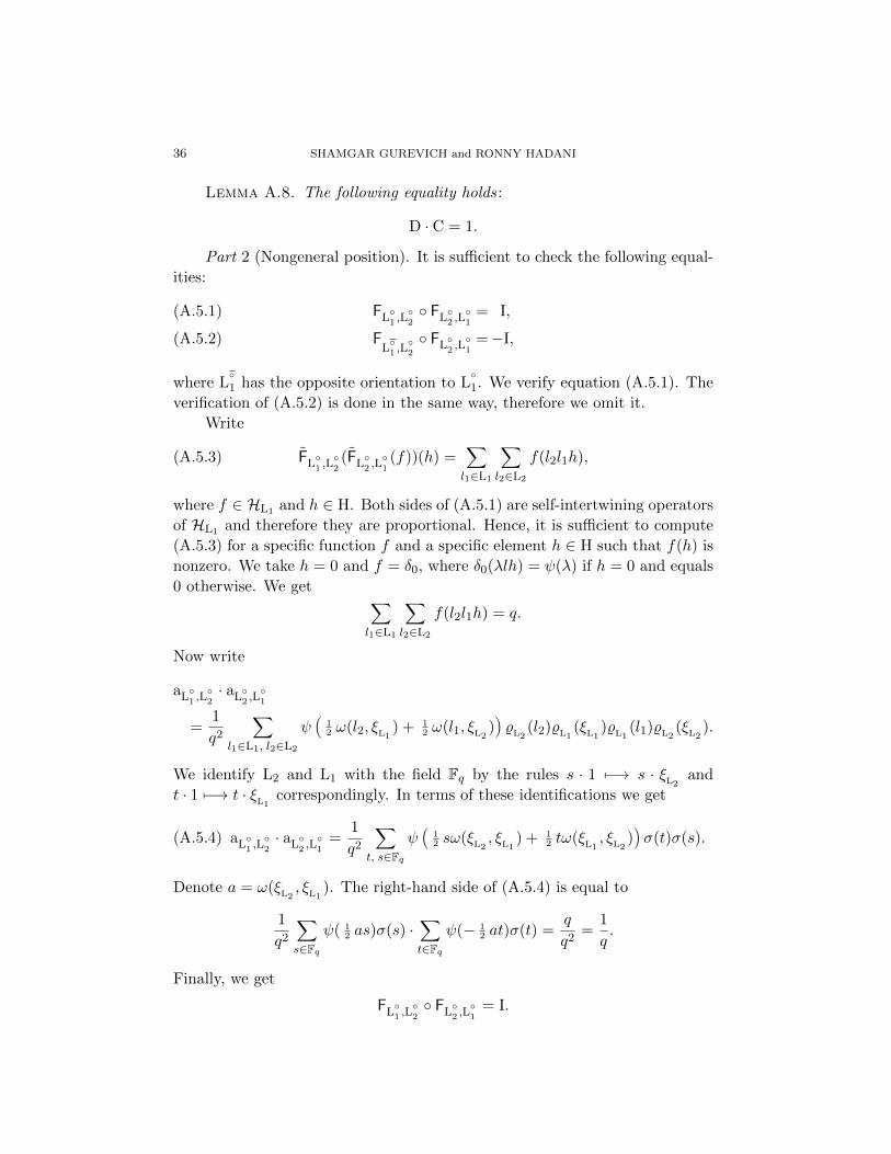
36 SHAMGAR GUREVICH and RONNY HADANI
Lemma A.8. The following equality holds :
D · C = 1.
Part 2 (Nongeneral position). It is sufficient to check the following equal-
ities:
FL1 ,L2 FL
2 ,L1
= I,(A.5.1)
FL1 ,L2
FL2 ,L1
=−I,(A.5.2)
where L1 has the opposite orientation to L
1. We verify equation (A.5.1). The
verification of (A.5.2) is done in the same way, therefore we omit it.
Write
(A.5.3) FL1 ,L2(FL
2 ,L1(f))(h) =
∑l1∈L1
∑l2∈L2
f(l2l1h),
where f ∈ HL1 and h ∈ H. Both sides of (A.5.1) are self-intertwining operators
of HL1 and therefore they are proportional. Hence, it is sufficient to compute
(A.5.3) for a specific function f and a specific element h ∈ H such that f(h) is
nonzero. We take h = 0 and f = δ0, where δ0(λlh) = ψ(λ) if h = 0 and equals
0 otherwise. We get ∑l1∈L1
∑l2∈L2
f(l2l1h) = q.
Now write
aL1 ,L2· aL
2 ,L1
=1
q2
∑l1∈L1, l2∈L2
ψÄ
12 ω(l2, ξL1
) + 12 ω(l1, ξL2
)ä%L2
(l2)%L1(ξL1
)%L1(l1)%L2
(ξL2).
We identify L2 and L1 with the field Fq by the rules s · 1 7−→ s · ξL2and
t · 1 7−→ t · ξL1correspondingly. In terms of these identifications we get
(A.5.4) aL1 ,L2· aL
2 ,L1
=1
q2
∑t, s∈Fq
ψÄ
12 sω(ξL2
, ξL1) + 1
2 tω(ξL1, ξL2
)äσ(t)σ(s).
Denote a = ω(ξL2, ξL1
). The right-hand side of (A.5.4) is equal to
1
q2
∑s∈Fq
ψ( 12 as)σ(s) ·
∑t∈Fq
ψ(− 12 at)σ(t) =
q
q2=
1
q.
Finally, we get
FL1 ,L2 FL
2 ,L1
= I.

PROOF OF THE KURLBERG-RUDNICK RATE CONJECTURE 37
Proof of Lemma A.6. The proof is by direct computation. Write
FL3 ,L1(f)(h) =
∑l3∈L3
f(l3h),(A.5.5)
FL3 ,L2
(FL2 ,L1(f))
(h) =∑l3∈L3
∑l2∈L2
f(l2l3h),(A.5.6)
where f ∈ HL1 and h ∈ H. Both (A.5.5) and (A.5.6) are intertwining operators
from HL1 to HL3 . Therefore they are proportional. In order to compute the
proportionality coefficient C it is enough to compute (A.5.5) and (A.5.6) for
specific f and specific e. We take h = 0 and f = δ0, where δ0(q,p, λ) = ψ(λ),
and get
FL3 ,L1(δ0) = 1,
FL3 ,L2
(FL2 ,L1(δ0)
)(0) =
∑l2+l3∈L1
ψ( 12 ω(l2, l3)).(A.5.7)
But the right-hand side of (A.5.7) is equal to∑l2∈L2
ψ( 12 ω(l2, rL3,L2
(l2))).
Proof of Lemma A.7. The proof is by direct computation. Write
aL3 ,L1
=1
q
∑l1∈L1
ψ( 12 ω(l1, ξL3
))%L1(l1)%L2
(ξL3),
aL3 ,L2· aL
2 ,L1
(A.5.8)
=1
q2
∑l1∈L1, l2∈L2
ψ( 12 ω(l1, ξL2
) + 12 ω(l2, ξL3
))%L1(l1)%L2
(ξL2)%L2
(l2)%L3(ξL3
).
The term ψ( 12 ω(l1, ξL2
) + 12 ω(l2, ξL3
)) is equal to
(A.5.9) ψ( 12 ω(l1, ξL2
− ξL3) + 1
2 ω(l2, ξL3)) · ψ( 1
2 ω(l1, ξL3)).
We are free to choose ξL3such that ξL2
− ξL3∈ L1. Therefore, using (A.5.9)
we get that the right-hand side of (A.5.8) is equal to
(A.5.10)1
q
∑l2∈L2
ψ( 12 ω(l2, ξL3
))%L2(ξL2
)%L2(l2) · aL
3 ,L1.
Now, substituting ξL3= −rL3,L2
(ξL2) in (A.5.10) we obtain
1
q
∑l2∈L2
ψ(− 12 ω(l2, rL3,L2
(ξL2)))%L2
(l2)%L2(ξL2
) · aL3 ,L1.

38 SHAMGAR GUREVICH and RONNY HADANI
Proof of Lemma A.8. Identify L2 with Fq by the rule t · 1 7−→ t · ξL2. In
terms of this identification we get
D =1
q
∑t∈Fq
ψ(− 12 ω(tξL2
, rL3,L2(ξL2
)))%(t),
C =∑t∈Fq
ψ( 12 ω(tξL2
, rL3,L2(tξL2
))).
Denote by a = ω(ξL2, rL3,L2
(ξL2)). Then
D =1
q
∑t∈Fq
ψ(− 12 at)%(t),
C =∑t∈Fq
ψ( 12 at
2).
Now, we have the following remarkable equality:∑t∈Fq
ψ( 12 at)%(t) =
∑t∈Fq
ψ( 12 at
2).
This, combined with C · C = q, gives the result.
This completes the proof of Part 2 and of Theorem A.3
Proof of Theorem A.5. The sheaf K is obtained by middle extension from
the open subvariety O of the sheaf KO. The sheaf KO is clearly geometri-
cally irreducible [dim(G) + 1]-perverse of pure weight 0. This implies that the
sheaf K is also geometrically irreducible [dim(G) + 1]-perverse of pure weight
Perv(K)=0.
Proof of Property 1. Assuming the validity of Property 2, we prove Prop-
erty 1. Restricting the sheaf K to the open subvariety O, and taking sheaf-
to-function correspondence, one obtains fK = fKO = K|Ø. Applying sheaf-to-
function correspondence to the multiplication isomorphism, we get that fK is
multiplicative. Finally, we use the fact that the set Ow ×H is a generating set
of G. Therefore, we have two functions K and fK that coincide on a gener-
ating set and satisfy the multiplication property. This implies that they must
coincide on the whole domain.
Proof of Property 2. What remains is to prove the multiplication property,
namely, Property 2. We will prove the left multiplication isomorphism. The
proof of the right multiplication isomorphism follows the same lines; therefore
we omit it. In the course of the proof we shall use the following auxiliary
sheaves:

PROOF OF THE KURLBERG-RUDNICK RATE CONJECTURE 39
• We sheafify the kernel Kπ using the formula (A.3.2) and obtain a sheaf
on H× A2:
(A.5.11) Kπ(h, x, y) = Lψ( 12
pq+px+λ) ⊗ δy=x+q,
where h = (q, p, λ), and we use the notation δ for the constant sheaf Q` on a
subvariety extended by zero.
• We sheafify the kernel Kρ when restricted to the set B × F2q using the
formula (A.3.1) and obtain a sheaf on the variety B×A2, which we denote by
KB,
(A.5.12) KB(b, x, y) = Lσ(a) ⊗Lψ(− 12ra−1x2) ⊗ δy=a−1x,
where b =Äa 0r a−1
ä.
•We will frequently make use of several other sheaves obtained by restric-
tions from KO, AO, KB and AB. Suppose X ⊂ Ow×H is a subvariety. Then
we define KX = KO|X×A2and AX = AO|X×A2
, the same when X ⊂ B. Finally,
we denote by δ0 the sky-scraper sheaf on A1 which corresponds to the delta
function at zero.
The proof of Property 2 will proceed in several steps:
Step 1. It is sufficient to prove the multiplication property separately
for the Weyl element w, an element b ∈ B and an element h ∈ H. This
follows from the Bruhat decomposition, Corollary A.12 below and the following
decomposition lemma.
Lemma A.9. There exist isomorphisms
KO ' KB ∗ Kw ∗ KU ∗ Kπ,
where U denotes the unipotent radical of B and w is the Weyl element.
Step 2. We prove Property 2 for the Weyl element, g = w. We want to
construct an isomorphism
(A.5.13) K|w ∗ K ' L∗wK.
Both sides of (A.5.13) are irreducible [dim(G)+1]-perverse since K|w∗ is essen-
tially a Fourier transform; therefore it is sufficient to construct an isomorphism
on the open subvariety O× = O∩wO where both sides are nonzero. This has
the advantage that over O× we have formulas for K, and moreover, Lw maps
O× into itself. We consider two decompositions:
O×'U× ×B×H,(A.5.14)
O×'U×w ×B×H,

40 SHAMGAR GUREVICH and RONNY HADANI
where U× = U − I and U denotes the unipotent radical of the standard
Borel. In terms of the above decompositions we have the following isomor-
phisms:
Claim A.10. There exist isomorphisms
1. KU (ubh) ' KU×(u) ∗ KB(b) ∗ Kπ(h),
2. KU (uwbh) ' KU×w(uw) ∗ KB(b) ∗ Kπ(h).
Now, when we restrict to O× and use the decomposition (A.5.14) our main
statement is the existence of an isomorphism
(A.5.15) Kw ∗ KU (ubh) ' KU (wubh).
Indeed, on developing the right-hand side of (A.5.15) we obtain
KU (wubh) =KU (uwwbh)
'KU×w(uww) ∗ KB(b) ∗ Kπ(h)
'Kw ∗ (KU×(u) ∗ KB(b) ∗ Kπ(h))
'Kw ∗ KU (ubh),
where uw = wuw−1. The first and third isomorphisms are applications of
Claim A.10, parts 2 and 1 respectively. The second isomorphism is a result of
associativity of convolution and the following central lemma:
Lemma A.11. There exists an isomorphism
(A.5.16) KU×w(uww) ' Kw ∗ KU×(u).
The following is a consequence of (A.5.13).
Corollary A.12. There exists an isomorphism
(A.5.17) K|B×H' KB ∗ Kπ.
Proof. On developing the left-hand side of (A.5.17) we obtain
K|B×H' Kw ∗ K|w−1B×H
' Kw ∗ (Kw−1 ∗ KB ∗ Kπ)
' (Kw ∗ Kw−1) ∗ KB ∗ Kπ' KB ∗ Kπ.
The first isomorphism is a consequence of (A.5.13). The second isomorphism
is a consequence of Lemma A.9. The third isomorphism is the associativity
property of convolution. The last isomorphism is a property of the Fourier
transform [20], that is, Kw ∗ Kw−1 ' I, where I is the kernel of the identity
operator.

PROOF OF THE KURLBERG-RUDNICK RATE CONJECTURE 41
Step 3. We prove Property 2 for element b ∈ B. Using Corollary A.12 we
have K|b ' KB|b = Kb. We want to construct an isomorphism
(A.5.18) Kb ∗ K ' L∗bK.
Since both sides of (A.5.18) are irreducible (shifted) perverse sheaves, it is
sufficient to construct an isomorphism on the open set O = Ow × H × A2.
Write
Kb ∗K|O ' Kb ∗KO ' Kb ∗ (KB ∗Kw ∗KU ∗Kπ) ' (Kb ∗KB) ∗ (Kw ∗KU ∗Kπ).
The first isomorphism is by construction. The second isomorphism is an ap-
plication of Lemma A.9. The third isomorphism is the associativity property
of the convolution operation between sheaves. From the last isomorphism we
see that it is enough to construct an isomorphism Kb ∗ KB ' L∗b(KB), where
Lb : B −→ B. The construction is an easy consequence of formula (A.3.1) and
the character sheaf property (A.4.3) of Lψ.
Step 4. We prove Property 2 for an element h ∈ H. We want to construct
an isomorphism
(A.5.19) K|h ∗ K ' L∗hK.
Both sides of (A.5.19) are irreducible [dim(G) + 1]-perverse. Therefore, it is
sufficient to construct an isomorphism on the open set O. This is done by a
direct computation, very similar to what has been done before, hence we omit
it. This concludes the proof of Theorem A.5.
Proof of Lemma A.9. We will prove the lemma in two steps.
Step 1. We prove that KO ' KOw ∗Kπ. In a more explicit form we want
to show
(A.5.20) AO ⊗ KO ' AOw ⊗ KOw ∗ KH.
It is sufficient to show the existence of an isomorphism KO ' KOw ∗ KH. On
developing the left-hand side of (A.5.20) we obtain
KO(g, h, x, y) = Lψ(R(g,h,x,y)).
On developing the right-hand side we obtain
KOw ∗ KH( (g, h) , x, y) = ∫z∈A1
KOw(g, x, z)⊗ KH(h, z, y)
= ∫A1
Lψ(Rg(x,z)) ⊗Lψ(Rh(z,y)) ⊗ δy=z−q
'Lψ(Rg(x,y−q)) ⊗Lψ(Rh(y−q,y))
'Lψ(Rg(x,y−q)+Rh(y−q,y))
= Lψ(R(g,h,x,y)).

42 SHAMGAR GUREVICH and RONNY HADANI
The only nontrivial isomorphism is the last one and it is a consequence of the
Artin-Schreier sheaf being a character sheaf on the additive group Ga.
Step 2. We prove that KOw ' KB ∗ Kw ∗ KU. In a more explicit form we
want to show that
AOw ⊗ KOw ' AB ⊗Aw ⊗AU ⊗ KB ∗ Kw ∗ KU,
where AB ⊗ KB = KB with AB(b) = Lσ(a) and KB(b, x, y) = Lψ(− 12ra−1x2) ⊗
δy=a−1x for a general element b =Äa 0r a−1
äin the group B (see (A.5.12)).
We will separately show the existence of two isomorphisms
KOw ' KB ∗ Kw ∗ KU,(A.5.21)
AOw 'AB ⊗Aw ⊗AU.(A.5.22)
Isomorphism (A.5.21). We have the decomposition, Ow w B × w × U.
Let b =Äa 0r a−1
äand u = ( 1 0
s 1 ) be general elements in the groups U and B
respectively. In terms of the coordinates (a, r, s) a general element in Ow is
of the form g =( as ars−a−1 r
). Developing the left-hand side of (A.5.21) in the
coordinates (a, r, s) we obtain
KOw(bwu, x, y) = Lψ(− 12a−1rx2+a−1xy− 1
2sy2).
On developing the right-hand side of (A.5.21) we obtain
KB ∗ Kw ∗ KU(bwu, x, y) = ∫z,z′∈A1
KB(b, x, z)⊗ Kw(w, z, z′)⊗ KU(u, z′, y)
= ∫z,z′∈A1
Lψ(− 12ra−1x2)
⊗ δx=az ⊗Lψ(zz′) ⊗Lψ(− 12sz′2) ⊗ δy=z′
' Lψ(− 12ra−1x2) ⊗Lψ(a−1xy) ⊗Lψ(− 1
2sy2)
' Lψ(− 12ra−1x2+a−1xy− 1
2sy2).
The last isomorphism is a consequence of the fact that the Artin-Schreier sheaf
is a character sheaf (A.4.3). Finally, we obtain isomorphism (A.5.21).
Isomorphism (A.5.22). On developing the left-hand side of (A.5.22) in
terms of the coordinates (a, r, s) we obtain
AOw(bwu) = G(ψa, σ)[2](1)
'G(ψ, σa−1)[2](1)
'Lσ(a−1) ⊗ G(ψ, σ)[2](1)
'Lσ(a) ⊗ G(ψ, σ)[2](1)
=AB ⊗Aw ⊗AU(bwu),

PROOF OF THE KURLBERG-RUDNICK RATE CONJECTURE 43
where G(ψs, σa) =∫A1 Lψ( 1
2sz)⊗Lσ(az) denotes the quadratic Gauss-sum sheaf.
The second isomorphism is a change of coordinates z 7→ z/a under the inte-
gration. The third isomorphism is a consequence of the Kummer sheaf Lσ
being a character sheaf on the multiplicative group Gm (A.4.4). The fourth
isomorphism is a specific property of the Kummer sheaf which is associated
to the quadratic character σ. This completes the construction of isomorphism
(A.5.22).
Proof of Claim A.10. This is carried out in exactly the same way as the
proof of the decomposition Lemma A.9: namely, by using the explicit formulas
of the sheaves KO,KB,Kπ and the character sheaf property of the sheaves Lψ
and Lσ.
Proof of Lemma A.11. First, we write isomorphism (A.5.16) in a more
explicit form
(A.5.23) AU×w ⊗ KU×w(uww) ' Aw ⊗AU× ⊗ Kw ∗ KU×(u).
Let u = ( 1 s0 1 ) ∈ U× be a nontrivial unipotent. Then uww = wu =
(0 1−1 −s
).
On developing the left-hand side of (A.5.23) we obtain
KU×w(uww, x, y) = Lψ( 12sx2+xy),
AU×w(uww) = G(ψ, σ)[2](1),
where G(ψs, σa) =∫A1 Lψ( 1
2sz) ⊗Lσ(az).
On developing the right-hand side of (A.5.23) we obtain
Kw ∗ KU×(u, x, y) = ∫z∈A1
Kw(x, z)⊗ KU×(u, z, y)
= ∫A1
Lψ(xz) ⊗Lψ(− 12s−1z2+s−1zy− 1
2s−1y2)
' ∫A1
Lψ(xz− 12s−1z2+s−1zy− 1
2s−1y2)
' ∫A1
Lψ(− 12s−1(z−sx−y)2) ⊗Lψ( 1
2sx2+xy)
' ∫A1
Lψ(− 12s−1z2) ⊗Lψ( 1
2sx2+xy).
By applying change of coordinates z 7→ sz under the last integration we obtain
(A.5.24) ∫A1
Lψ(− 12s−1z2) ⊗Lψ( 1
2sx2+xy) ' ∫
z∈A1
Lψ(− 12sz2) ⊗Lψ( 1
2sx2+xy).
Now,
(A.5.25) Aw ⊗AU×(u) = G(ψ, σ)[2](1)⊗ G(ψs, σ)[2](1).

44 SHAMGAR GUREVICH and RONNY HADANI
Combining (A.5.24) and (A.5.25) we obtain that the right-hand side of (A.5.23)
is isomorphic toÇG(ψs, σ)[2](1)⊗ ∫
A1
Lψ(− 12sz2)
å⊗(G(ψ, σ)[2](1)⊗Lψ( 1
2sx2+xy)
).
The main argument is the existence of the following isomorphism:
G(ψs, σ)[2](1)⊗ ∫A1
Lψ(− 12sz2) ' Q`,
which is a direct consequence of the following lemma:
Lemma A.13 (Main lemma). There exists a canonical isomorphism of
sheaves on Gm
∫A1
Lψ( 12sz) ⊗Lσ(z) ' ∫
A1
Lψ( 12sz2),
where s ∈ Gm.
Proof. The parameter s does not play any essential role in the argument.
Therefore, it is sufficient to prove
(A.5.26) ∫A1
Lψ(z) ⊗Lσ(z) ' ∫A1
Lψ(z2).
Define the morphism p : Gm −→ Gm, p(x) = x2. The morphism p is an etale
double cover. We have p∗Q` ' Lσ⊕Q`. Now on developing the left-hand side
of (A.5.26) we obtain
∫A1
Lψ(z) ⊗Lσ(z) = π!(Lψ ⊗Lσ) ' π!(Lψ ⊗ (Lσ ⊕Q`)).
The first step is just a translation to conventional notation, where π stands
for the projection π : Gm −→ pt. The second isomorphism uses the fact that
π!Lψ ' 0. Next,
π!(Lψ ⊗ (Lσ ⊕Q`)) ' π!(Lψ ⊗ p∗Q`) ' π!p∗Lψ = ∫
A1
Lψ(z2).
This completes the proof of proposition A.11.
Appendix B. Proofs section
We fix the following notation. Let ~ = 1p , where p is a fixed prime 6= 2, 3.
Consider the lattice Λ∗ of characters of the torus T and the quotient vector
space V = Λ∗/pΛ∗. The integral symplectic form on Λ∗ is specialized to give
a symplectic form on V, i.e., ω : V × V −→ Fp. Fix ψ : Fp −→ C∗ as the
additive character ψ(t) = e2πi~t, and let A~ be “the algebra of functions on the
quantum torus” and Γ ' SL2(Z) its group of symmetries.

PROOF OF THE KURLBERG-RUDNICK RATE CONJECTURE 45
B.1. Proof of Theorem 2.3. Basic set-up: Let (π~ ,H~) be a representation
of A~, which is a representative of the unique irreducible class which is fixed
by Γ (cf. Theorem 2.2). Let ρ~ : Γ −→ PGL(H~) be the associated projective
representation. Here we give a proof that ρ~ can be linearized in a unique way
which factors through the quotient group Γp ' SL2(Fp)Γ //
ρ~@
@@@@
@@@@
@@Γp
ρ~
GL(H~).
The proof will be given in several steps.
Step 1. Uniqueness. The uniqueness of the linearization follows directly
from the fact that the group SL2(Fp), p 6= 2, 3, has no characters.
Step 2. Existence.16 The main technical tool in the proof of existence is
a construction of a finite-dimensional quotient of the algebra A~. Let Ap be
the unital associative algebra generated over C by the symbols s(v) | v ∈ Vand the relations
(B.1.1) s(u)s(v) = ψ( 12 ω(u, v))s(u+ v), s(0) = 1.
The algebra Ap is nontrivial and the vector space V gives on it a standard
basis. In fact, Ap is isomorphic to a quotient C[H] ⊗C[Z]
C of the group algebra
of H, where H is the Heisenberg group defined in A.1.2, Z its center, and the
tensor product is formed using the homomorphism C[Z] → C defined by ψ.
We have the following map:
s : V −→ Ap, v 7→ s(v).
The group Γp acts on Ap by automorphisms through its action on V. The
epimorphism Λ∗ V induces a homomorphism of algebras
(B.1.2) q : A~ −→ Ap.
The homomorphism (B.1.2) respects the actions of the group of symmetries Γ
and Γp respectively. This is summarized in the following commutative diagram:
(B.1.3)
Γ×A~ −−−−→ A~
(p,q)
y q
yΓp ×Ap −−−−→ Ap,
where p : Γ −→ Γp is the canonical quotient map.
16This statement and its proof work more generally for all Planck constants of the form
~ = M/N, with M,N co-prime integers, and N odd. One should replace then the finite Field
Fp with the finite ring Z/NZ.

46 SHAMGAR GUREVICH and RONNY HADANI
Step 3. Next, we construct an explicit representation of Ap:
πp : Ap −→ End(H).
Let V = V1⊕
V2 be a Lagrangian decomposition of V. In our case V is two-
dimensional, therefore V1 and V2 are linearly independent lines in V. Take
H = S(V1) to be the vector space of complex valued functions on V1. For an
element v ∈ V define
(B.1.4) πp(v) = ψ(− 12 ω(v1, v2))Lv1Mv2 ,
where v = v1 + v2 is a direct decomposition v1 ∈ V1, v2 ∈ V2, Lv1 is the
translation operator defined by v1
Lv1(f)(x) = f(x+ v1), f ∈ S(V1)
and Mv2 is a notation for the operator of multiplication by the function Mv2(x)
= ψ(ω(x, v2)). One checks that the formulas given in (B.1.4) satisfy the re-
lations (B.1.1) and thus constitute a representation of the algebra Ap, and
this representation corresponds to the induced representation IndHV2
Cψ of H
considered in A.1.3.
As a consequence of constructing πp we automatically proved that Ap is
nontrivial. It is well known that all linear operators on S(V1) are linear com-
binations of translation operators and multiplication by characters. Therefore,
πp : Ap −→ End(H) is surjective. As dim(Ap) ≤ p2, πp is a bijection. This
means that Ap is isomorphic to a matrix algebra Ap 'Mp(C).
Step 4. Completing the proof of existence. The group Γp acts on Ap.Therefore, it acts on the category of its representations. However, Ap is iso-
morphic to a matrix algebra; therefore it has unique irreducible representation,
up to isomorphism. This is the standard representation of dimension p. But
dim(H) = p, therefore πp is an irreducible representation and its isomorphism
class is fixed by Γp so that we have a pair
πp : Ap−→End(H),
ρp : Γp−→PGL(H)
satisfying the Egorov identity
ρp(B)πp(v)ρp(B−1) = πp(Bv),
where B ∈ Γp and v ∈ Ap.It is a well known general fact (attributed to I. Schur) that the group Γp,
where p is an odd prime, has no nontrivial projective representations. This

PROOF OF THE KURLBERG-RUDNICK RATE CONJECTURE 47
means that ρp can be linearized17 to give
ρp : Γp −→ GL(H).
Now take
H~ = H, π~ = πp q, ρ~ = ρp p.Because q intertwines the actions of Γ and Γp (cf. diagram (B.1.3)) we see that
π~ and ρ~ are compatible; namely, the Egorov identity is satisfied
ρ~(B)π~(f)ρ~(B−1) = π~(fB),
where B ∈ Γp and f ∈ A~. Here the notation π~(fB) means to apply any pre-
image B ∈ Γ of B ∈ Γp on f . In particular, this implies that the isomorphism
class of π~ is fixed by Γ. Since such a representation π~ is unique up to an
isomorphism, (Theorem 2.2), our desired object has been obtained.
B.2. Proof of Lemma 4.3. Basic set-up: Let (π~ ,H~) be a representation
of A~, which is a representative of the unique irreducible class which is fixed
by Γ (cf. Theorem 2.2). Let ρ~ : Γp −→ GL(H~) be the associated honest
representation of the quotient group Γp (see Theorem 2.3 and Proof B.1).
Recall the notation Y0 = Γp × Λ∗. We consider the function F : Y0 −→ Cdefined by the following formula:
(B.2.1) F (B, ξ) = Tr(ρ~(B)π~(ξ)),
where ξ ∈ Λ∗ and B ∈ Γp. We want to show that F factors through the
quotient set Y = Γp ×V
Y0
F AAA
AAAA
AA// Y
F
C.
The proof is immediate, when we take into account the construction given in
Section B.1. Let πp be the unique (up to isomorphism) representation of the
quotient algebra Ap. As was stated in B.1, π~ is isomorphic to πp q, where
q : A~ −→ Ap is the quotient homomorphism between the algebras. This
means that π~(ξ) = πp(q(ξ)) depends only on the image q(ξ) ∈ V, and formula
(B.2.1) solves the problem.
B.3. Proof of Theorem 4.4. Basic set-up: In this section we use the nota-
tion of Section B.1 and Appendix A. Set Y = Sp×V and let α : Sp×Y −→ Y
denote the associated action map. Let F : Y −→ C be the function appearing
in the statement of Theorem 4.4, i.e., F (B, v) = Tr(ρp(B)πp(v)), where B ∈ Sp
17See Appendix A for an independent proof based on “The method of canonical Hilbert
space”.

48 SHAMGAR GUREVICH and RONNY HADANI
and v ∈ V. We use the notation V, Sp and Y to denote the corresponding al-
gebraic varieties. We construct a Weil object F ∈ Dbc(Y) having the properties
1–4 stated in Theorem 4.4.
Construction of the sheaf F . We use the notation of Appendix A. Let H
be the Heisenberg group. As a set we have H = V×Fq. The group structure is
given by the multiplication rule (v, λ) ·(v′, λ′) = (v+v′, λ+λ′+ 12 ω(v, v′)). We
fix a section s : V 99K H, s(v) = (v, 0). The group Sp acts by automorphisms
on the group H, through its tautological action on the vector space V; i.e.,
g · (v, λ) = (gv, λ). We define the semi-direct product G = SpnH and consider
the map (Id, s) : Y −→ G. We use the notation H and G to denote the
corresponding algebraic varieties.
Let K be the Weil representation sheaf (see Theorem A.5). Define
F = Tr(K|Y),
where Tr is defined in analogy to the operation of taking trace in the set-
theoretic framework; that is, we take
F(g, v) =
∫x∈A1
K(g, v, x, x),
where we use the notation∫x∈A1 to denote integration with compact support
along the x-variable. We prove that the sheaf F satisfies Properties 1–4.
Proof of Property 2. Property 2 follows easily. One should observe that
the collection of operators πp(v)v∈V extends to a representation of the group
H, which we will also denote by πp. The representations ρp and πp glue to
a single representation ρp n πp of the semi-direct product G. It is a direct
verification, that the representation ρpnπp is isomorphic to the representation
ρn π constructed in Appendix A. Hence, we can write
fF = fTr(K|Y ) = Tr(fK|Y ) = Tr(K|Y) = F.
In the above equation we use the fact that the operation of taking the
geometric trace commutes with sheaf-to-function correspondence. This proves
Property 2.
Proof of Property 3. This principally follows from the multiplication prop-
erty of the sheaf K (Theorem A.5, Property 2). More precisely, using the
multiplication property we obtain the following isomorphism:
K|S ∗ K ∗ K|S−1' L∗SR∗S−1K,
where LS , RS−1 denotes left multiplication by S and right multiplication by
S−1 on the group G, respectively. Next,
α∗SF ' Tr(α∗SK|Y) ' Tr(L∗SR∗S−1K|Y) ' Tr(K|S ∗ K|Y ∗ K|S−1
).
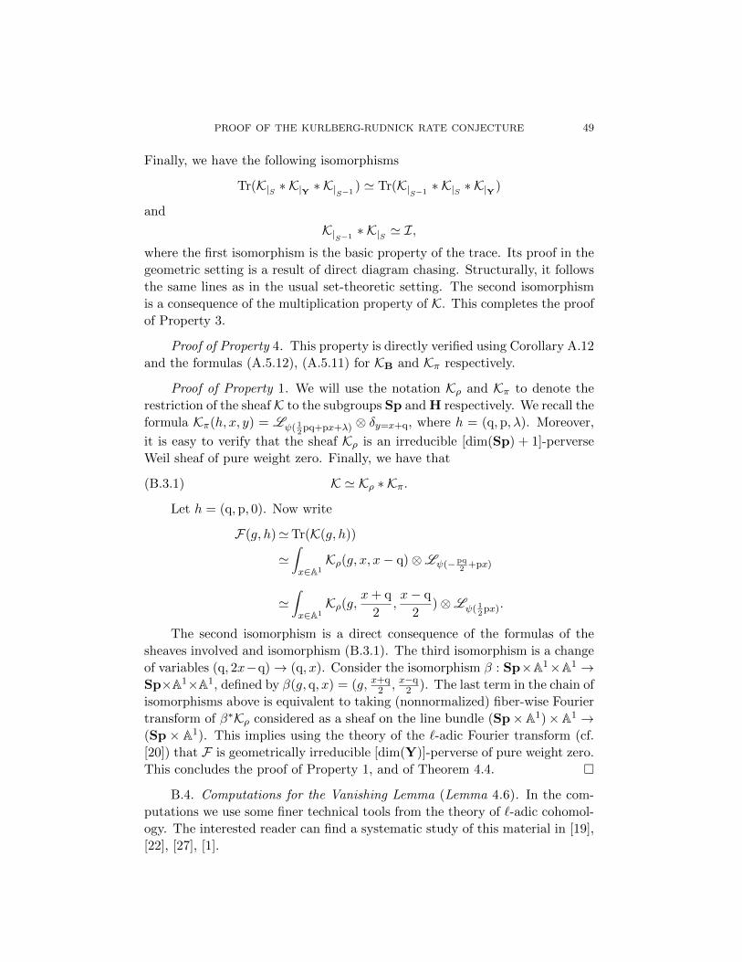
PROOF OF THE KURLBERG-RUDNICK RATE CONJECTURE 49
Finally, we have the following isomorphisms
Tr(K|S ∗ K|Y ∗ K|S−1) ' Tr(K|S−1
∗ K|S ∗ K|Y)
and
K|S−1∗ K|S ' I,
where the first isomorphism is the basic property of the trace. Its proof in the
geometric setting is a result of direct diagram chasing. Structurally, it follows
the same lines as in the usual set-theoretic setting. The second isomorphism
is a consequence of the multiplication property of K. This completes the proof
of Property 3.
Proof of Property 4. This property is directly verified using Corollary A.12
and the formulas (A.5.12), (A.5.11) for KB and Kπ respectively.
Proof of Property 1. We will use the notation Kρ and Kπ to denote the
restriction of the sheaf K to the subgroups Sp and H respectively. We recall the
formula Kπ(h, x, y) = Lψ( 12
pq+px+λ) ⊗ δy=x+q, where h = (q, p, λ). Moreover,
it is easy to verify that the sheaf Kρ is an irreducible [dim(Sp) + 1]-perverse
Weil sheaf of pure weight zero. Finally, we have that
(B.3.1) K ' Kρ ∗ Kπ.
Let h = (q,p, 0). Now write
F(g, h)'Tr(K(g, h))
'∫x∈A1
Kρ(g, x, x− q)⊗Lψ(−pq2
+px)
'∫x∈A1
Kρ(g,x+ q
2,x− q
2)⊗Lψ( 1
2px).
The second isomorphism is a direct consequence of the formulas of the
sheaves involved and isomorphism (B.3.1). The third isomorphism is a change
of variables (q, 2x−q)→ (q, x). Consider the isomorphism β : Sp×A1×A1 →Sp×A1×A1, defined by β(g, q, x) = (g, x+q
2 , x−q2 ). The last term in the chain of
isomorphisms above is equivalent to taking (nonnormalized) fiber-wise Fourier
transform of β∗Kρ considered as a sheaf on the line bundle (Sp×A1)×A1 →(Sp × A1). This implies using the theory of the `-adic Fourier transform (cf.
[20]) that F is geometrically irreducible [dim(Y)]-perverse of pure weight zero.
This concludes the proof of Property 1, and of Theorem 4.4.
B.4. Computations for the Vanishing Lemma (Lemma 4.6). In the com-
putations we use some finer technical tools from the theory of `-adic cohomol-
ogy. The interested reader can find a systematic study of this material in [19],
[22], [27], [1].

50 SHAMGAR GUREVICH and RONNY HADANI
We identify the standard torus T ⊂ SL2 with the group Gm. Fix a
nontrivial character sheaf18 Lχ on Gm. Denote by Lψ a nontrivial character
sheaf on Ga. Fix λ, µ ∈ A1 with λ ·µ 6= 0. Consider the variety X = Gm−1,the sheaf
E = Lψ( 12a+1a−1
λ·µ) ⊗Lχ,(B.4.1)
on X and the canonical projection pr : X −→ pt. Note that E is a nontrivial
one-dimensional local system on X. The proof of the lemma will be given in
several steps
Step 1. Vanishing. We want to show that Hi(pr!E) = 0 for i = 0, 2. By
definition
H0(pr!E) = Γ(Y, j!E),
where j : X → Y is the imbedding of X into a compact curve Y. The
statement follows since
Γ(Y, j!E) = Hom(Q`, j!E).
It is easy to see that any nontrivial morphism Q` → j!E should be an isomor-
phism on X; hence Hom(Q`, j!E) = 0.
For the second cohomology we have
H2(pr!E) = H−2(Dpr!E)∗ = H−2(pr∗DE)∗ = Γ(X, DE [−2])∗,
where D denotes the Verdier duality functor19 and [−2] is the translation
functor. The first equality follows from the definition of D, the second equality
is the Poincare duality and the third equality easily follows from the definitions.
Again, since the sheaf DE [−2] is a nontrivial one-dimensional local system on
X we have
Γ(X, DE [−2]) = Hom(Q`, DE [−2]) = 0.
Step 2. Dimension. We claim that dim H1(pr!E) = 2. The (topological)
Euler characteristic χ(pr!E) of the sheaf pr!E is the integer defined by the
formula
χ(pr!E) =∑i
(−1)idim Hi(pr!E).
Hence, from the vanishing of cohomologies (Step 1) we deduce
18That is, a one-dimensional local system on Gm that satisfies the property m∗Lχ wLχ Lχ, where m : Gm ×Gm → Gm is the multiplication morphism.
19In the vector bundle interpretation, one might think of D as the operation of taking the
dual vector bundle with the dual connection.

PROOF OF THE KURLBERG-RUDNICK RATE CONJECTURE 51
Substep 2.1. It is sufficient to show that χ(pr!E) = −2. The actual com-
putation of the Euler characteristic χ(pr!E) is done using the Ogg-Shafarevich-
Grothendieck formula (see [7], [27], [19, Chap. 2], and references therein)
rk(E) · χ(pr!Q`)− χ(pr!E) =∑
y∈Y−XSwany(E).(B.4.2)
Here rk(E) = 1 is the rank of the sheaf E , Q` denotes the constant sheaf on
X, and Y = P1 is the smooth compactification of X. In other words, this
formula expresses the difference of rk(E) · χ(pr!Q`) from χ(pr!E) as a sum
of local contributions, called Swan conductors. We will not to give here the
formal definition of the Swan conductor (see [19], [20], [27]), but instead we
will formulate some of the properties and known results that are needed for
our calculations.
In our case χ(pr!Q`) = −1, and by using formula (B.4.2) we get
Substep 2.2. It is enough to show that Swan0(E) + Swan1(E) + Swan∞(E)
= 1. We would like now to understand the effect of the tensor product on the
Swan conductor. Choose a point y ∈ Y −X, and let L1, L2 ∈ Dbc(X) be two
sheaves with L1 being lisse (smooth) in a neighborhood of y. We have
(B.4.3) Swany(L1 ⊗ L2) = rk(L1) · Swany(L2).
In particular, using property (B.4.3) and the explicit formula (B.4.1) of
the sheaf E , we deduce that
Swan1(E) = Swan∞(Lψ),
Swan∞(E) = Swan∞(Lχ),
Swan0(E) = Swan0(Lχ).
Substep 2.3. We have Swan∞(Lψ)=1, and Swan∞(Lχ) + Swan0(Lχ)=0.
By applying the Ogg-Shafarevich-Grothendieck formula to the Artin-Schreier
sheaf Lψ on A1 and the projection pr : A1 −→ pt, we find that
Swan∞(Lψ) = χ(pr!Q`)− χ(pr!Lψ) = 1− 0 = 1.(B.4.4)
Finally, we apply the formula (B.4.2) to the sheaf Lχ on Gm and the projection
pr : Gm −→ pt and conclude
Swan∞(Lχ) + Swan0(Lχ) = χ(pr!Q`)− χ(pr!Lχ) = 0− 0 = 0.(B.4.5)
Note that, in (B.4.4) and (B.4.5) we use the fact that pr!Lψ and pr!Lχ are
the 0-objects in Dbc(pt).
This completes the computations of the Vanishing Lemma.

52 SHAMGAR GUREVICH and RONNY HADANI
References
[1] A. A. Beilinson, J. Bernstein, and P. Deligne, Faisceaux pervers, in Anal-
ysis and Topology on Singular Spaces, I (Luminy, 1981), Asterisque 100, Soc.
Math. France, Paris, 1982, pp. 5–171. MR 0751966.
[2] J. Bernstein, private communication, Max-Planck Institute, Bonn, Germany
(August, 2004).
[3] M. V. Berry, Regular and irregular semiclassical wavefunctions, J. Phys. A 10
(1977), 2083–2091. MR 0489542. Zbl 0377.70014. Available at http://stacks.iop.
org/0305-4470/10/2083.
[4] , Semiclassical mechanics of regular and irregular motion, in Chaotic Be-
havior of Deterministic Systems (Les Houches, 1981), North-Holland, Amster-
dam, 1983, pp. 171–271. MR 0724465. Zbl 0571.70018.
[5] A. Bouzouina and S. De Bievre, Equipartition of the eigenfunctions of quan-
tized ergodic maps on the torus, Comm. Math. Phys. 178 (1996), 83–105.
MR 1387942. Zbl 0876.58041. doi: 10.1007/BF02104909.
[6] M. Degli Esposti, S. Graffi, and S. Isola, Classical limit of the quan-
tized hyperbolic toral automorphisms, Comm. Math. Phys. 167 (1995), 471–507.
MR 1316757. Zbl 0822.58022. doi: 10.1007/BFb0091519.
[7] P. Deligne, Applications de la formule des traces aux sommes trigonometriques,
in Cohomologie Etale, SGA 4 12 , Lecture Notes in Math. 569, Springer-Verlag,
New York, 1977, pp. 168–232. Zbl 0349.10031. doi: 10.1007/BFb0091523.
[8] , Rapport sur la formule des traces, in Cohomologie Etale, Seminaire
de Geometrie Algebrique du Bois-Marie SGA 4 12 , Lecture Notes in Math. 569,
Springer-Verlag, New York, 1977, pp. 76–109. Zbl 0349.14009. doi: 10.1007/
BFb0091519.
[9] , La conjecture de Weil. II, Inst. Hautes Etudes Sci. Publ. Math. 52 (1980),
137–252. MR 0601520. Zbl 0456.14014. Available at http://www.numdam.org/
item?id=PMIHES 1980 52 137 0.
[10] , Metaplectique, 1982, A letter to Kadhdan.
[11] F. Faure, S. Nonnenmacher, and S. De Bievre, Scarred eigenstates for
quantum cat maps of minimal periods, Comm. Math. Phys. 239 (2003), 449–492.
MR 2000926. Zbl 1033.81024. doi: 10.1007/s00220-003-0888-3.
[12] D. Gaitsgory, Informal introduction to geometric Langlands, in An Introduc-
tion to the Langlands Program (Jerusalem, 2001), Birkhauser, Boston, MA, 2003,
pp. 269–281. MR 1990383. Zbl 1111.11308.
[13] P. Gerardin, Weil representations associated to finite fields, J. Algebra 46
(1977), 54–101. MR 0460477. Zbl 0359.20008. doi: 10.1016/0021-8693(77)
90394-5.
[14] A. Grothendieck, Formule de Lefschetz et rationalite des fonctions L, Sem.
Bourbaki 9 (1964).
[15] S. Gurevich and R. Hadani, The two dimensional Hannay-Berry model, 2003.
arXiv math-ph/0312039.
[16] , Application of the Weil representation: diagonalization of the discrete
Fourier transform, in New Developments in Lie Theory and Geometry, Contemp.

PROOF OF THE KURLBERG-RUDNICK RATE CONJECTURE 53
Math. 491, Amer. Math. Soc., Providence, RI, 2009, pp. 167–178. MR 2537057.
Zbl 1180.43003.
[17] J. H. Hannay and M. V. Berry, Quantization of linear maps on a torus-
Fresnel diffraction by a periodic grating, Phys. D 1 (1980), 267–290. MR 0602111.
Zbl 1194.81107. doi: 10.1016/0167-2789(80)90026-3.
[18] R. E. Howe, On the character of Weil’s representation, Trans. Amer. Math. Soc.
177 (1973), 287–298. MR 0316633. Zbl 0263.22014. doi: 10.2307/1996597.
[19] N. M. Katz, Gauss sums, Kloosterman sums, and monodromy groups, Annals
of Math. Studies 116, Princeton Univ. Press, Princeton, NJ, 1988. MR 0955052.
Zbl 0675.14004.
[20] N. M. Katz and G. Laumon, Transformation de Fourier et majoration de
sommes exponentielles, Inst. Hautes Etudes Sci. Publ. Math. (1985), 361–418.
MR 0823177. Zbl 0603.14015.
[21] D. Kazhdan, private communication, hebrew University, Jerusalem, Israel
(March, 2004).
[22] R. Kiehl and R. Weissauer, Weil Conjectures, Perverse Sheaves and l’adic
Fourier Transform, Ergeb. Math. Grenzgeb. 42, Springer-Verlag, New York, 2001.
MR 1855066. Zbl 0988.14009.
[23] H. D. Kloosterman, The behaviour of general theta functions under the mod-
ular group and the characters of binary modular congruence groups. I, Ann. of
Math. 47 (1946), 317–375. MR 0021032. Zbl 0063.03262. doi: 10.2307/1969082.
[24] P. Kurlberg, private communication, Chalmers University, Gothenburg, Swe-
den (September, 2003).
[25] P. Kurlberg and Z. Rudnick, Hecke theory and equidistribution for the
quantization of linear maps of the torus, Duke Math. J. 103 (2000), 47–77.
MR 1758239. Zbl 1013.81017. doi: 10.1215/S0012-7094-00-10314-6.
[26] , On the distribution of matrix elements for the quantum cat map, Ann.
of Math. 161 (2005), 489–507. MR 2150390. Zbl 1082.81054. doi: 10.4007/
annals.2005.161.489.
[27] G. Laumon, Semi-continuite du conducteur de Swan (d’apres P. Deligne), in
The Euler-Poincare Characteristic (French), Asterisque 83, Soc. Math. France,
Paris, 1981, pp. 173–219. MR 0629128. Zbl 0504.14013.
[28] G. Lion and M. Vergne, The Weil Representation, Maslov Index and Theta
Series, Progr. Mat. 6, Birkhauser, Mass., 1980. MR 0573448. Zbl 0444.22005.
[29] J. S. Milne, Etale Cohomology, Princeton Math. Series 33, Princeton Univ.
Press, Princeton, N.J., 1980. MR 0559531. Zbl 0433.14012.
[30] D. Mumford, Tata Lectures on Theta. III, Progr. Math. 97, Birkhauser,
Boston, MA, 1991, with the collaboration of Madhav Nori and Peter Norman.
MR 1116553. Zbl 0744.14033. doi: 10.1007/978-0-8176-4579-3.
[31] M. A. Rieffel, Noncommutative tori—a case study of noncommutative differ-
entiable manifolds, in Geometric and Topological Invariants of Elliptic Operators
(Brunswick, ME, 1988), Contemp. Math. 105, Amer. Math. Soc., Providence, RI,
1990, pp. 191–211. MR 1047281. Zbl 0713.46046.

54 SHAMGAR GUREVICH and RONNY HADANI
[32] Z. Rudnick, The quantized cat map and quantum ergodicity, Lecture at the
MSRI conference “Random Matrices and their Applications”, Berkeley, June 7–
11, 1999.
[33] , On quantum unique ergodicity for linear maps of the torus, in Euro-
pean Congress of Mathematics, Vol. II (Barcelona, 2000), Progr. Math. 202,
Birkhauser, Basel, 2001, pp. 429–437. MR 1905382. Zbl 1025.37017.
[34] P. Sarnak, Arithmetic quantum chaos, in The Schur Lectures (1992) (Tel Aviv),
Israel Math. Conf. Proc. 8, Bar-Ilan Univ., Ramat Gan, 1995, pp. 183–236.
MR 1321639. Zbl 0831.58045.
[35] A. I. Snirel′man, Ergodic properties of eigenfunctions, Uspehi Mat. Nauk 29
(1974), 181–182. MR 0402834. Zbl 0324.58020.
[36] A. Weil, Sur les Courbes Algebriques et les Varietes qui s’en dEduisent, Actu-
alites Sci. Ind. 1041, Hermann et Cie., Paris, 1948. Zbl 0036.16001.
[37] , Sur certains groupes d’operateurs unitaires, Acta Math. 111 (1964), 143–
211. MR 0165033. Zbl 0203.03305. doi: 10.1007/BF02391012.
(Received: April 8, 2005)
(Revised: October 21, 2009)
University of California, Berkeley, CA
Current address : University of Wisconsin, Madison, WI
E-mail : [email protected]
University of Chicago, Chicago, IL
Current address : The University of Texas at Austin, Austin, TX
E-mail : [email protected]