project work: implementation of soot model for aachenbomb...

CFD WITH OPENSOURCE SOFTWARE

A COURSE AT CHALMERS UNIVERSITY OF TECHNOLOGYTAUGHT BY HAKAN NILSSON

Project work:

Implementation of soot model foraachenBomb tutorial

Developed for OpenFOAM-3.0.x

Author:VIGNESH PANDIANMUTHURAMALINGAM

Peer reviewed by:HAKAN NILSSON

JOHANNES TORNELL

Disclaimer: This is a student project work, done as part of a course where OpenFOAM andsome other OpenSource software are introduced to the students. Any reader should be awarethat it might not be free of errors. Still, it might be useful for someone who would like learnsome details similar to the ones presented in the report and in the accompanying files. Thematerial has gone through a review process. The role of the reviewer is to go through the

tutorial and make sure that it works, that it is possible to follow, and to some extent correct thewriting. The reviewer has no responsibility for the contents.

January 24, 2016

Contents

1 Learning outcomes 1

2 Implementation of soot model for aachenBomb tutorial 22.1 Introduction to aachenBomb Tutorial . . . . . . . . . . . . . . . . . . . . . . . . . . . 2

2.1.1 Copy aachenBomb tutorial . . . . . . . . . . . . . . . . . . . . . . . . . . . . 22.1.2 Solver . . . . . . . . . . . . . . . . . . . . . . . . . . . . . . . . . . . . . . . . 2

2.2 Geometry and initial conditions . . . . . . . . . . . . . . . . . . . . . . . . . . . . . . 32.3 Input files . . . . . . . . . . . . . . . . . . . . . . . . . . . . . . . . . . . . . . . . . . 42.4 Introduction to soot modelling . . . . . . . . . . . . . . . . . . . . . . . . . . . . . . 82.5 Addition to the OpenFOAM soot model code . . . . . . . . . . . . . . . . . . . . . . 82.6 Implementation and execution of the code . . . . . . . . . . . . . . . . . . . . . . . . 82.7 Post- processing . . . . . . . . . . . . . . . . . . . . . . . . . . . . . . . . . . . . . . . 122.8 Output Files included for reference . . . . . . . . . . . . . . . . . . . . . . . . . . . . 182.9 Study Questions . . . . . . . . . . . . . . . . . . . . . . . . . . . . . . . . . . . . . . . 18

References 20

ii

Chapter 1

Learning outcomes

In this report, the reader will :

• obtain introduction to combustion solvers in openFOAM and insight into the aachenbombcase

• learn how to set up the aachenbomb case

• learn how to modify a soot model implemented in the radiation library and use it for theaachenBomb case

• learn some basic post processing techniques in openFOAM paraView

1

Chapter 2

Implementation of soot model foraachenBomb tutorial

2.1 Introduction to aachenBomb Tutorial

The aachenBomb case is the simulation of combustion inside a constant volume chamber thatmimics the begining of power stroke in a 4 stroke engine. The experimental setup of the com-bustion chamber is in RWTH Aachen university, and the operating conditions are in accordancewith the Engine Combustion Network [[1]].

2.1.1 Copy aachenBomb tutorial

The commands to copy the aachenBomb case to run folder of user directory are given below. Thecase can be referred to by the reader to check all the files that will be described in the followingsections.

OF30xcdmkdir $WM_PROJECT_USER_DIR/mkdir $FOAM_RUNcd $WM_PROJECT_DIR/cp -r tutorials/lagrangian/sprayFoam/aachenBomb/ $FOAM_RUN

All the implementations in this tutorial are done in OpenFOAM-3.0.x. The aachenBomb casefolder has 4 folders, namely - 0, system, constant and chemkin respectively.The 0 folder contains all the files to set initial values for some of the fields.The system folder contains the files - blockMeshDict, controlDict, fvSchemes and fvSolution. TheblockMeshDict is a dictionary file containing specification of the geometry in order to create themesh. The controlDict file is the control dictionary containing the parameters to control simula-tion settings for the case. The fvSchemes file has the settings for finite volume schemes used toperform some mathematical operation on the solved variables (gradient is one example for themathematical operations). The fvSolution file contains specific settings of finite volume solverfor some of the variables.The third folder in the case file is the constant folder. This folder contains all the input files thatare needed to load the libraries, models and sub models used by the case.The chemkin folder in the case file contains two files. These are the input for chemical reactionmechanism : chemkin.inp; and the file therm.inp, which includes the input to calculate thermo-physical properties of the compounds involved in the reaction.

2.1.2 Solver

The sprayFoam Solver The aachenBomb case is solved using the sprayFoam solver. The spray-Foam solver has the lagrangian particle tracking option. It is a transient PIMPLE type of solverfor solving compressible flows with spray parcels. It can solve for laminar or turbulent cases.

2

CHAPTER 2. IMPLEMENTATION OF SOOT MODEL FOR AACHENBOMB TUTORIAL 3

In this tutorial the solver solves for compressible turbulent flow. There is another variant of thesprayFoam solver for engine applications named engineFoam (Unlike the constant volume case,it solves for moving mesh mimicing the movement of piston for a real engine case).The file sprayFoam.c includes the code for sprayFoam solver and it can be found in

$WM_PROJECT_DIR/applications/solvers/lagrangian/sprayFoam

In the file sprayFoam.c the lagrangian particles (in this case it is the fuel particles) are solvedby calling the function parcels.evolve() . Following this, the Eulerian phase equations aresolved (Eulerian phase is the carrier phase which is air in this case) for momentum, mass fractionand energy respectively. These equations are invoked by the solver. It can be seen in the code as:

#include "UEqn.H"#include "YEqn.H"#include "EEqn.H"

Solver options for engine combustion simulations in openFoam The different types of solversavailable for internal combustion engines are summarised in table 2.1. The difference between thesprayEngineFoam and engineFoam is that the engineFoam solver does not solve for lagrangianspray parcels. There is no treatment of droplets or fuel injection in the engineFoam solver. Thedifference between sprayEngineFoam and coldEngineFoam is that coldEngine foam does notsolve for lagrangian spray and it does not include combustion. The difference between cold-EngineFoam and engineFoam is that the coldEngineFoam does not solve for combustion.

Table 2.1: Combustion solvers in OpenFOAMSolver FunctionalitysprayFoam constant volume combustion solver for compressible flows involving spray parcelssprayEngineFoam moving piston engine solver for compressible flows involving spray parcelscoldEngineFoam solver for cold flow(without combustion) for internal combustion enginesengineFoam Solver for combustion in internal combustion engines

2.2 Geometry and initial conditions

As mentioned before the geometry of aachenBomb case is similar to the constant volume com-bustion chamber in RWTH Aachen. The geometry is a cuboid with height(+ve y-axis) 0.1m andbase 0.02x0.02m (figure 2.1). The injector is placed 5mm below the top of the chamber (at a height0.995m from the bottom plane) in order to avoid boundary effects on the injected fluid. The fluidthat is injected is n-Heptane (C7H16).


0.100

Figure 2.1: Computational domain

The user should run blockMesh utility in order to create the mesh for the above mentioned ge-ometry . This is done as follows:

runcd aachenBombblockMesh

The initial conditions of the aachenBomb case are summarised in table 2.2

Table 2.2: Initial conditions for aachenBomb caseGas temperature in the constant volume chamber 800KGas pressure in the constant volume chamber 50barGas velocity in the constant volume chamber 0 m/sFuel n-HeptaneO2 concentration in the constant volume chamber 23.4%N2 concentration in the constant volume chamber 76.6%Injection temperature 320Kε 90 (uniform internal field, walls:epsilonWallFunction)k 1 (uniform internal field, walls:kqRWallFunction)

2.3 Input files

The user can see the input files for the case in the constant folder of the aachenBomb case thatwas earlier on copied to the run directory. The input files along with their significance, is shownin table 2.3.Some of the important input files are discussed below.

sprayCloudProperties The sprayCloudProperties file can be found in the constant folder ofthe aachenBomb case. The sprayCloudProperties input file contains the submodels to set upthe lagrangian spray model. The frequently used submodels along with the important inputparameters are now summarised. These submodels can be seen in the section subModels of thesprayCloudProperties file. Some of the important subModels are discussed below:


Table 2.3: Input files for the aachenBomb caseInput file FunctionalitysprayCloudProperties contains inputs for the lagrangian spray modelthermophysicalProperties contains inputs for the thermophysical modelsradiationProperties contains inputs for radiation, absorption- emission and soot modelsChemistryProperties Specifies the chemistry solver and option to switch on/off the chemical

reactionscombustionProperties contains inputs for combustion model and option to switch on/off

combustionturbulenceProperties contains inputs for turbulence model and option to switch on/off turbulence

sprayCloudProperties: injectionModels injectionModels is one of the options present in spray-CloudProperties file. This option specifies one of the 9 injector types, geometry, position, flowRatePro-file of the injector and direction of injection. The flowRateProfile can either be given as an input inthe same file itself in two columns or as a separate file containing the two columns (useful in caseof long duration injections). The two columns are time (s) and mass flow rate (kg/s) respectively.There are 9 injector model types and they can be found in:

$FOAM_SRC/lagrangian/intermediate/submodels/Kinematic/InjectionModel/

In this tutorial the coneNozzleInjection model is used. This is model used in order to deal withinjection of conical fuel sprays typical in engine combustion situations. The angle of the cone,location and direction of the injector are specified by user input in the sprayCloudProperties file.

sprayCloudProperties: phaseChangeModel The phaseChangeModel contains the submodelfor evaporation of the spray droplets. There are 3 phase change models and they can be found in

$FOAM_SRC/lagrangian/intermediate/submodels/Reacting/PhaseChangeModel/.

In this tutorial, the liquidEvaporationBoil model is used. The liquidEvaporationBoil model asthe name suggests is used to model the boiling and evaporation of the injected fuel spray. Asit can be seen in the sprayCloudproperties file, there are two input coefficients for the liquidE-vaporationBoil model. enthalpyTransfer defines how enthalpy is transferred between the liquid(fuel) and the carrier (surrounding air). The two types of enthalpy transfer are latentHeat andenthalpyDifference. Following this there is another coefficient call activeLiquids which specifiesthe liquid fuel that is being used (n-Heptane in this case).

sprayCloudProperties: breakupModel The breakup model contains the submodels for sec-ondary breakup of the droplets. There are 7 submodels for secondary breakup and they can befound in

$FOAM_SRC/lagrangian/spray/submodels/BreakupModel/

In this tutorial, the PilchErdman breakup model is used. By default in the sprayCloudPropertiesfile, the breakup model is ReitzDiwakar. This should be changed as:

breakupModel PilchErdman;

In the same file, after the coefficients for liquidEvaporationBoilCoeffs section, add the following:

PilchErdmanCoeffs{

solveOscillationEq yes;B1 0.375;

B2 0.2274;

}

After the addition, this part should look as follows:


liquidEvaporationBoilCoeffs{

enthalpyTransfer enthalpyDifference;

activeLiquids ( C7H16 );}

PilchErdmanCoeffs{solveOscillationEq yes;B1 0.375;B2 0.2274;}

ReitzDiwakarCoeffs{

solveOscillationEq yes;Cbag 6;Cb 0.785;Cstrip 0.5;Cs 10;

}

The ReitzDiwakarCoeffs can be removed if the user wants. This will not make a difference as thecompiler now knows that the breakup model is PilchErdman.The PilchErdman model deals with the secondary breakup of the droplets with time, based oncertain empirical parameters. There are two coefficients for the model namely B1 and B2. Theseare constants used in the equations of PilchErdman correlations for determining droplet diameterand breakup time constant respectively.It should be noted that the type of breakup model chosen does not have any connection to therequisites of soot model. The author performed earlier works on droplet breakup study usingPilchErdman model and decided to continue using the same breakup model for this project. Butusing the PilchErdman model will make it easier for the reader to cross check the plots discussedlater in the report.

radiationProperties and changes needed to be made to include soot model The radiationProp-erties file is present in the constant folder of the case directory. It is an input file that contains theinputs for type of radiation model and the inputs for the radiation submodels. The submodelsof radiation are: absorptionEmissionModel, scatterModel and sootModel. Inside the file, the ra-diation is by default switched off. The radiation needs to be switched on in order to include thesootModel. The entire radiationProperties file should be replaced with the following content:

/*--------------------------------*- C++ -*----------------------------------*\| ========= | || \\ / F ield | OpenFOAM: The Open Source CFD Toolbox || \\ / O peration | Version: 3.0.x || \\ / A nd | Web: www.OpenFOAM.org || \\/ M anipulation | |\*---------------------------------------------------------------------------*/FoamFile{

version 3.0;format ascii;class dictionary;location "constant";object radiationProperties;

}// * * * * * * * * * * * * * * * * * * * * * * * * * * * * * * * * * * * * * //

radiation on;

radiationModel P1;

//Number of flow iterations per radiation iterationsolverFreq 10;

absorptionEmissionModel none;


scatterModel none;

sootModel mymixtureFractionSoot<gasHThermoPhysics>;

mymixtureFractionSootCoeffs{

nuSoot 0.055;Wsoot 12;

}

// ************************************************************************* //

Since the sootModel is a submodel in radiationModel, it is called through the radiationModel.The soot library is also present in the radiation library.Therefore it is needed to switch on theradiation and specify any one of the radiationModel in order to call the sootModel. In this imple-mentation, the P1 radiation model is used.The sootModel used here is mymixtureFractionSootModel.There are two user defined coefficientsfor the soot model. The coefficient nuSoot indicated the number of moles of soot in the combus-tion reaction. The coefficient Wsoot is the molecular weight of soot. Further explanation of sootmodel follows in the section: Introduction to soot modelling.

thermophysicalProperties The thermophysical properties provide input for the thermophysi-cal models. The file is present inconstant/thermophysicalProperties in the case folder.It provides the inputs - mixture type, the method by which to calculate thermophysical properties(in this case it is janaf). In the janaf method, all the thermophysical properties -Cp, H and S are de-rived from NASA polynomials. The NASA polynomials calculate the above mentioned proper-ties based on NASA coefficients. The input for these coefficients is present in chemkin/therm.datin the case folder. This file name and path is specified in the thermophysicalProperties file. It issuggested to look at [3] for details on these coefficients. Apart from this, the location of chemistryfile chemkin.inp is also specified in the thermophysicalProperties file. In this case the chemistryfile is present in chemkin/chemkin.inp in the case folder. The chemkin.inp file used in this tuto-rial for combustion of n-Heptane, is shown in figure 2.2

Figure 2.2: chemkin.inp

There are 5 inputs in this file. The three numbers 5.00E+8, 0.0 and 15780 represent A, b and Ea inthe Arrhenius rate equation.

kf = AT b.exp(−Ea

RT) (2.1)

, where A is constant for pressure dependence, T is the temperature and Ea is the activationenergy. The Arrhenius rate equation determines the rate of a chemical reaction as a function


of temperature, pressure and activation energy. The numbers 0.25 and 1.5 denote the forwardreaction order of n-Heptane and oxygen respectively.

2.4 Introduction to soot modelling

The soot model used in this tutorial is based on the mixturefraction soot model existing in Open-FOAM [2]. This soot model is used in the fireFoam tutorial for combustion of methane.The aachenBomb tutorial does not use any soot model. Soot model for combustion studies isrequired to analyse the pollutant formation. This was a motivation to develop the soot model forthe aachenBomb tutorial. Also there is a further contribution in code to the existing model, thatwill be discussed later. However, this is a first step, and further refinements should be made fordetailed studies.The mixturefraction soot model is a simple state model. It does not solve for transport equationof soot. Instead it calculates the soot mass fraction based on the CO2 mass fraction at all cells foreach timestep.The generalised single step reaction including soot production is

nufFuel + (nuOx)Ox = (nuP )P + (nuSoot)soot. (2.2)

nuf, nuOx, nuP and nuSoot are the number of moles of fuel, oxidizer, product and soot respec-tively. In the case of this tutorial, the single step reaction is

(nuf)C7H16 + (nuOx)O2 = (nuP1)CO2 + (nuP2)H2O + (nuSoot)soot. (2.3)

The number of moles of soot, nuSoot also known as the soot yield is specified by the user. Themass fraction of soot is calculated as

soot[cellI] = sootMax ∗ (Y CO2[cellI]/Y CO2stoch). (2.4)

Here, sootMax is the maximum soot that can be produced. It is calculated from the single stepreaction for n-Heptane shown in eqn (2.3)

2.5 Addition to the OpenFOAM soot model code

The drawback of the above mentioned soot model is that, it calculates soot at all times whenCO2 is produced. However, soot is produced only in rich conditions of the fuel (when the fuelexceeds the stochiometric fuel value required for complete combustion). This means that soot isproduced only if :

Y C7H16[cellI] > Y C7H16stoch, (2.5)

where YC7H16 is the mass fraction of the fuel (n-Heptane).Further details about modification to the code is discussed in the next section.

2.6 Implementation and execution of the code

Implementation Before we can execute the case the following implementations must be done.

1. Ensure that the aachenBomb case is copied to run folder of user directory as explained inthe subsection: Copy aachenBomb tutorial; in the first section.

2. Copy the radiation library to user directory

3. Rename and modify the soot library

4. Compile and dynamically link soot library


1. Ensure that the aachenBomb case is copied to run folder as explained in the first section

2. Copy the radiation library to user directory Since the soot submodel is present in the radia-tion library, it is required to copy the radiation library to user directory. This is done as follows:

OF30xcd $WM_PROJECT_DIRcp -r --parents src/thermophysicalModels/radiation/ $WM_PROJECT_USER_DIR/cd $WM_PROJECT_USER_DIR/src/thermophysicalModels/radiation/submodels/sootModel/

3. Rename and modify the soot library We will implement a modified soot model by changingthe existing mixtureFraction model with the addition of equation (2.5). To do this, first we startby renaming the existing soot model to mymixtureFraction. This is done as follows:

mv mixtureFractionSoot mymixtureFractionSootcd mymixtureFractionSoot/mv mixtureFractionSoot.C mymixtureFractionSoot.Cmv mixtureFractionSoot.H mymixtureFractionSoot.Hsed -i s/mixtureFractionSoot/mymixtureFractionSoot/g mymixtureFractionSoot.Hsed -i s/mixtureFractionSoot/mymixtureFractionSoot/g mymixtureFractionSoot.Csed -i s/mixtureFractionSoot/mymixtureFractionSoot/g mixtureFractionSoots.C

Once the soot model is renamed, we need to edit the file mymixtureFractionSoot.C and mymix-tureFractionSoot.H to include the modifications. First we start with mymixtureFractionSoot.C.We need to open the file mymixtureFractionSoot.C and search for

if (mappingFieldName_ == "none")

From that point on, include the following code:

if (mappingFieldName_ == "none"){

const label index = reaction.rhs()[0].index;const label index1 = reaction.lhs()[0].index;mappingFieldName_ = mixture_.Y(index).name();mappingFieldName1_ = mixture_.Y(index1).name();

}

const label mapFieldIndex = mixture_.species()[mappingFieldName_];mapFieldMax_ = mixture_.Yprod0()[mapFieldIndex];Info << "Value of mappingFieldName_:"<<mappingFieldName_<<endl;Info << "Value of mapFiledMax_:"<<mapFieldMax_<<endl;

}

// * * * * * * * * * * * * * * * * Destructor * * * * * * * * * * * * * * * //

template<class ThermoType>Foam::radiation::mymixtureFractionSoot<ThermoType>::˜mymixtureFractionSoot(){}

// * * * * * * * * * * * * * * * Member Functions * * * * * * * * * * * * * //

template<class ThermoType>void Foam::radiation::mymixtureFractionSoot<ThermoType>::correct(){

const volScalarField& mapField =mesh_.lookupObject<volScalarField>(mappingFieldName_);

const volScalarField& mapField1 =mesh_.lookupObject<volScalarField>(mappingFieldName1_);

forAll (mapField1,i){

if( mapField1[i] >0.068) // Ystoch=0.068 for fuel n-Heptane, calculated from single step combustion of n-Heptane in air (76.6% N2 and 23.4% O2 by weight)

soot_[i] = sootMax_*(mapField[i]/mapFieldMax_);


elsesoot_[i] = 0;}

}

// * * * * * * * * * * * * * * * * * * * * * * * * * * * * * * * * * * * * * //

The addition to the code is explained as follows. In order to add equation (2.5), the mass frac-tion of fuel should (Y C7H16) should be obtained. The variable index1 stores the index offuel which is 0 (The fuel is the first term in left hand side of equation (2.2)). The variablemappingF ieldName1 stores the name of the fuel which in this case is C7H16 (first term in lefthand side of equation(2.3)). The volume scalar field mapField1 stores the value of fuel massfraction in all the cells.

Finally, the variable mappingFieldName1_ must be declared in the file mymixtureFraction-Soot.H. This is done as follows: search the file mymixtureFractionSoot.H for

word mappingFieldName_;

In the next line enter the following text:

//- Name of the field mapping the fuelword mappingFieldName1_;

Save the file and exit.

4. Compile and dynamically link soot library Final step to be followed is to compile the sootlibrary. But, before we compile we need to change the name and location of the executable radi-ationModels library. This is done as follows

cd $WM_PROJECT_USER_DIRcd src/thermophysicalModels/radiation/sed -i s/FOAM_LIBBIN/FOAM_USER_LIBBIN/g Make/filessed -i s/libradiationModels/libmyradiationModels/g Make/filessed -i s/mixtureFractionSoot/mymixtureFractionSoot/ Make/files

The last line should also be added. This is because not only have we changed the name sootmodel files but also the name of the soot model folder.Once this is done we can compile the library as follows:

cd $WM_PROJECT_USER_DIRcd src/thermophysicalModels/radiation/wcleanwmake libso

At the end of this compilation, the output libmyradiationModels should be placed in the userlibrary.The next step is to dynamically link this library so that it can be called by the solver duringexecution. This is done as follows.

runcd aachenBombvi system/controlDict

Once in the aachenBomb case folder, and with the controlDict file opened, enter the following asthe last line of code:

libs ("libmyradiationModels.so");


Execution The steps to be followed before the aachenBomb case with the modified soot modelcan be executed are shown below and the explanation of these steps follows:

1. The required files for initial conditions of soot model and radiation model, should be placedin the 0/ folder of the case directory. These files are: soot and G (for incident radiation).

2. The entry for Gfinal (required by the radiation model) should be included in the fvSolutionfile.

3. The thermophysicalProperties file (present in constant folder of case directory) should beedited to include the inputs for single step reaction.

4. Ensure that the breakup model is changed in sprayCloudproperties file

5. Ensure that the radiationProperties file (input file required by the radiation model presentin constant folder of case directory) is edited as explained in section : Input files; underthe paragraph named: radiationProperties and changes needed to be made to include sootmodel.

6. Ensure that the blockMesh command is executed as explained before in section: Geometryand initial conditions

7. The last step would be to execute the command: sprayFoam to run the aachenBomb case.

The above mentioned steps are now explained in detail.

1. Required files for initial conditions of soot model and radiation model The soot modelrequires a soot input folder in the initial conditions. For this, the soot file has to be copied fromthe smallPoolFire2D case. This is done as follows:

runcd aachenBombcp -r $FOAM_TUTORIALS/combustion/fireFoam/les/smallPoolFire2D/0/soot 0/

The radiation model requires input folder G(incident radiation). For this, the file has to be copiedfrom the smallPoolFire2D case. This is done as follows:

runcd aachenBombcp -r $FOAM_TUTORIALS/combustion/fireFoam/les/smallPoolFire2D/0/G 0/

2. The entry for Gfinal The entry Gfinal should also be included in system/fvSolution folder.It should be included in the solvers after rho. The part to be included is shown:

GFinal{solver PCG;preconditioner DIC;tolerance 1e-05;relTol 0.1;}

3. The thermophysicalProperties file should be edited The combustion of fuel with air isrepresented by single step chemical reaction as shown in equation (2.2). The compiler shouldknow this information. For this purpose we have to edit the thermophysicalProperties file. Thisfile is present in the constant folder. The entire content should be replaced with the followingcode :


/*--------------------------------*- C++ -*----------------------------------*\| ========= | || \\ / F ield | OpenFOAM: The Open Source CFD Toolbox || \\ / O peration | Version: 3.0.x || \\ / A nd | Web: www.OpenFOAM.org || \\/ M anipulation | |\*---------------------------------------------------------------------------*/FoamFile{

version 2.0;format ascii;class dictionary;location "constant";object thermophysicalProperties;

}// * * * * * * * * * * * * * * * * * * * * * * * * * * * * * * * * * * * * * //

thermoType{

type hePsiThermo;//mixture reactingMixture;mixture singleStepReactingMixture;transport sutherland;thermo janaf;energy sensibleEnthalpy;equationOfState perfectGas;specie specie;

}

CHEMKINFile "$FOAM_CASE/chemkin/chem.inp";

CHEMKINThermoFile "$FOAM_CASE/chemkin/therm.dat";newFormat yes;

inertSpecie N2;

fuel C7H16;

liquids{

C7H16{

defaultCoeffs yes;}

}

solids{

// none}

// ************************************************************************* //

Basically what we have changed is the option reactingMixture to singleStepReactingMixture andincluded the option fuel.

Change the breakup model in sprayCloudproperties file Ensure that the breakup model ischanged in the sprayCloudproperties file as explained previously in the section Input files underthe paragraph: sprayCloudProperties: breakupModel.

Ensure steps 5 and 6 are performed as explained in previous sections

Executing the case The case is now ready to be run. The case is executed by the commandsprayFoam while in the case folder.

2.7 Post- processing

creating glyph to observe lagrangian droplets In order to view the lagrangian droplet, first aVTK file is created. When inside the case folder, execute,


foamToVTKparaFoam

Following this, the two VTK files should be loaded in paraFoam (On opening from the File menu,the VTK folder can be seen. Inside this folder the vtk file for the continuous case can be seen. Nav-igating one level further into the lagrangian folder and then one more level into the sprayCloudfolder, the vtk file for lagrangian phase can be seen. Both these vtk files should be loaded ). Thesetup for making glyph is shown in figure 2.3.

Figure 2.3: screenshot of glyph settings

The glyph created to view the lagrangian droplets is shown in figure 2.4.


Figure 2.4: glyph of fuel droplets created at t=0.35ms

Alternatively glyph can be viewed without converting to vtk.The ParaFoam version used by theauthor is 4.4. This version can handle lagrangian particles without converting to vtk. This was asimple method with the steps listed as follows:

• ParaFoam should be opened in the case folder.

• Time should be increased by 1 value from 0 to 1. (This is simply because in time 0, the la-grangian particles are not available)

• In the properties tab, the option apply should be clicked. Doing this will display the inter-nalMesh.

• In the properties tab, under the option Mesh Parts, by default the option ’internalMesh’ isselected. This should be changed. The ’internalMesh’ option should be unchecked andonly the ’sprayCloud - lagrangian’ option should be selected. (ensure that all other optionsare deselected).

• In the properties tab, under the option Lagrangian Fields, ’d’ should be checked to view par-ticle diameter.

• The apply option should be clicked in the properties tab. In the dropdown list, the option’vtkBlockColors’ is selected by default. This should be changed to ’d’, in order to view thelagrangian particles.

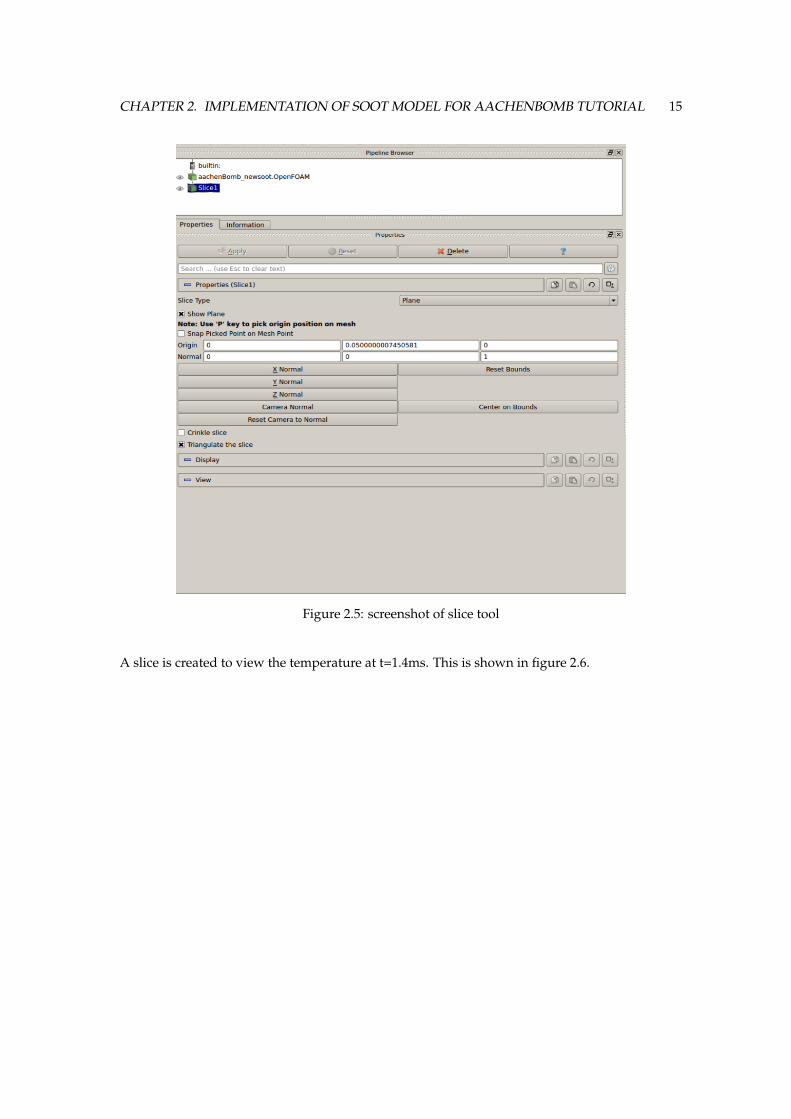
Another tool in paraFoam is ’slice’. Slice is a useful tool to look at the information in a givenplane of interest. In this case it is the slice take normal to the z-plane cutting through the middleof the geometry. A screenshot of the slice window is shown in figure 2.5.


Figure 2.5: screenshot of slice tool

A slice is created to view the temperature at t=1.4ms. This is shown in figure 2.6.


Figure 2.6: slice of temperature at t=1.4 ms.

Finally, a comparison of the soot obtained using the existing OpenFOAM soot model and themodified soot model, is shown in figure 2.7 and 2.8.

0.0002829

0.0005658

0.0008487

0.000e+00

1.132e-03

soot

Figure 2.7: slice of soot from existing model at t=1.4ms


0.00026455

0.00052911

0.00079366

0.000e+00

1.058e-03

soot

Figure 2.8: slice of soot from the modified model at t=1.4ms

The difference between the existing and the modified soot model is clearly seen. The modifiedsoot model has a thinner region of formation of soot, concentrated more towards the centre. Thisis according to what we would expect because, in the centre the fuel has lesse acess to oxygenthan at periphery. This makes it a fuel rich region enabling the production of soot. The sootformation in the existing model (figure 2.7) is similar to CO2 formation. The CO2 formation att=1.4ms is shown in figure 2.9. The fact that the new soot model predicts soot over a thinner

0.047271

0.094541

0.14181

0.000e+00

1.891e-01

CO2

Figure 2.9: slice of CO2 at t=1.4ms

region can also be seen from a plot along the x-axis for y=0.05m(mid-section) and z=0. This plotwas obtained using the sampleDict tool. ref figure 2.10.


xdistance

0 0.005 0.01 0.015 0.02

Soot m

ass fraction

×10-3

0

0.2

0.4

0.6

0.8

1

1.2 existing soot modelmodified soot model

Figure 2.10: soot production versus x distance

2.8 Output Files included for reference

For the purpose of saving time and quickly observing the output, some executables are includedwith the tutorial for reference. The executables include the result of running the case with 4random time steps. One of the timestep included corresponds to the plots displayed in the Post-processing section. In any case if there is a problem encountered with compiling or executingthe case, the given executables can be used. The executable named V ignesh case.tar.gz has thefollowing contents:

• aachenBomb folder

• aachenBomb newsoot folder

• libmyradiationModels.so library

Two cases are included in the executable. These are aachenBomb and aachenBomb newsoot re-spectively. This can be used to observe the difference between the original case and the onemodified with the inclusion of soot model.The library libmyradiationModels.so is also given in the executable. If the user wants to savetime for compiling, then instead the given library file can be used. This should be copied andpasted in the user library folder.

2.9 Study Questions

• Which solver is used for constant volume combustion applications?


• Which file contains the input parameters for sootModel?

• What are the initial files and changes that need to be made before executing the aachenBombcase?

• In which library is the code for sootModel included?

Bibliography

[1] Engine combustion network, Sandia, U.S.A; website: http : //www.sandia.gov/ecn/.

[2] OpenFOAM v2.3.0: Physical Modelling: section: Combustion/Pyrolysis ; website: http ://www.openfoam.org/version2.3.0/physical −modelling.php.

[3] NASA polynomials and coefficients; website: http ://combustion.berkeley.edu/gri mech/data/nasa plnm.html

20

project work: implementation of soot model for aachenbomb...

Documents