Project THEMIS Technical Report No. 17

WIND-TUNNEL MODELING OF FLOW AND DIFFUSION OVER AN URBAN COMPLEX

by

F. H. Chaudhry

and

J. E. Cermak

Prepared under

Office of Naval Research

Contract No. N00014-68-A-0493-000l

Project No. NR 062-4l4/6-6-68(Code 438)

U. S. Department of Defense

Washington, D.C.

"This document has been approved for public release and sale; its distribution is unlimited."

Fluid Dynamics and Diffusion Laboratory College of Engineering

Colorado State University Fort Collins, Colorado

May, 1971

CER70-7lFHC-JEC24

Ull.,Ol 05751.,5

DISCLAIMER

THE FINDINGS IN THIS DOCUMENT ARE NOT TO BE CONSTRUED AS AN OFFICIAL DEPARTMENT OF THE ARMY POSITION UNLESS SO DESIGNATED BY OTHER AUTHORIZED DOCUMENTS. THE USE OP TRADE NAMES IN THIS REPORT DOES NOT CONSTITUTE AN OFFICIAL ENDORSEMENT OR APPROVAL OF THE USE OF SUCH COMMERCIAL HARDWARE OR SOFTWARE. THIS REPORT MAY NOT BE CITED FOR PURPOSES OF ADVERTISEMENT.

DISPOSITION INSTRUCTIONS

DESTROY THIS REPORT WHEN NO LONGER NEEDED DO NOT RETURN IT TO THE ORIGINATOR

ABSTRACT

The purpose of this study is to explore and test the powerful

potential of wind-tunnel modeling as an alternative to the more expensive

and tedious full-scale urban diffusion experiments.

A model of the city of Fort Wayne was constructed to a horizontal

scale of 1:4000 and a vertical scale of 1:2000. Flow and diffusion over

the model was studied in the environmental wind tunnel of the Fluid

Dynamics and Diffusion Laboratory at Colorado State University. If the

roughness and the heat-island effects modeled properly, and the

approach flows made similar, the flow over the model city was found to

conform to that in the field. The pattern of the heat island over Fort

Wayne is reproduced almost exactly in the model. Simulation of diffusion

from an aerial line source was accomplished by traversing a continuously

emitting source of Krypton-85 upwind of the city. The measured dosages

of this tracer over the city compare well with the corresponding field

data except immediately downwind from the source where the downdraft

from the disseminating aircraft becomes significant in the field. The

model is found to give same overall picture of the effect of the city on

dispersion process as that observed in the field. The results show that

the heat island effect vitiates the environment by bringing pollutants

down from elevated releases through enhanced vertical mixing. The model

results compare reasonably with approximate theory of Smith (1957).

The results of this study have proved that it is indeed possible to

simulate the flow over a city and obtain useful information, relatively

inexpensively, on urban diffusion. This investigation opens the way for

studies of air-pollution problems for purposes of urban planning. The

ii

location of industrial sites relative to major topographical features,

the location of freeways through existing cities, the grouping of tall

buildings in an urban-development program, or even the judicious placing

of parks, residential and industrial areas in an entirely new city to

minimize air pollution potentials under adverse meteorological conditions

can be studied systematically.

iii

ACKNOWLEDGMENT

This study was initiated by Deseret Test Center (Dugway Proving

Ground) as an attempt to determine the feasibility of wind tunnel

modeling of the meteorological regimes of cities as an alternative to

making extensive field measurements. A copy of the original field

study at Fort Wayne, Indiana by Hilst and Bowne (sponsored by Deseret

Test Center through program IT062111A128) was provided to Colorado

State University by Deseret Test Center for comparative purposes and is

normally available only in the Department of Defense. Funding for the

wind tunnel study was provided by program IT06211lAl28 through contract

DAAB07-68-C-0423, which is monitored by the United States Army Electronics

Command (ECOM) and administered by the United States Army Materiel

Command (AMC).

The authors wish to acknowledge the help of all the personnel of

the Fluid Mechanics Program, College of Engineering, Colorado State

University, who were associated with this study.

Special thanks are due to Dr. G. Hsi for his contributions at the

early stages of this work when the problems appeared insurmountable.

The efforts of Mr. R. Johansen contributed greatly to the model construc­

tion. Our discussions with Messers J. Garrison, Fluid Dynamics

Laboratory Supervisor and R. Asmus, Machine Shop Supervisor during design

of equipment contributed very much toward performing the quasi­

instantaneous diffusion experiments and are greatly appreciated.

Appreciation is expressed to Mr. S. Sethuraman and Mr. K. Nambudripad

for their assistance in data collection and analysis. The writers are

thankful to Dr. M. Julliand for his participation in the diffusion

iv

experiments. Thanks are due to Miss H. Akari for excellent drafting and

to Mary Grace Smith for careful typing.

v

Table

I.

II.

III.

IV.

LIST OF TABLES

Surface Dosages (with heating) . . . .

Surface Dosages (without heating) ..

Fixed Source Concentrations . . . . .

Surface Air Temperatures . . .

vi

Page

40

41

42

43

LIST OF FIGURES

Figure

1. Environmental Wind Tunnel . . . . . 44

2. Free Stream Velocity Variation in the Longitudinal Direction .. 45

3. Transverse Velocity Distribution at x=20 and 32 ft. 46

4. Traversing Arrangement . . . . . . . . . . . . . . . 47

5. Schematic Diagram of the Tracer Release System. . . . . 48

6. Sampling System . . . . .. .. . . . . • . • • 49

7. Model Lay-Out and Diffusion Sampling Stations .50

8. Layout of Nichrome-wire Heating Elements ...• 51

9. Comparison of Model and Prototype Velocity Profiles Approaching the City . . . .. .................... 52

10. Comparison of Model and Prototype Turbulence Intensities .... 53

11. Development of Velocity Profiles over Model City ........ 54

12. Development of Turbulence Intensity Profiles over the Model City . . . . . . . . . . . • . . . . . • . • • .. • 55

13. Development of Temperature Profiles over the Model City . . 56

14. "Heat Island" Generated Over the Model City . . • 57

15.

16.

"Heat Island" Observed over Fort Wayne

Smoke Diffusion over the Model ...•.•

. . . . . 58

. • 59

17. Surface Dosage Pattern Observed over the Model. The Numbers on the IS~Dosage Lines Indicate Non-Dimensional Dosage Defined on Page 28 . . . . . . . • . . • • . • • • • . . • • • . . . . 60

18. Surface Dosage Pattern Observed in Fort Wayne During Trial 65-06-G2. The Numbers on the Iso-Dosage Lines Indicate Non­Dimensional Dosage Defined on Page 28 . . . • • • . • . • . • . 61

19. Average Surface Dosage Observed in Fort Wayne City and Rural Areas During 70 Trials, in Particle-Min/Liter (After Hilst and Bowne 1966) . . . . • . . . • . . . . . • .. .... . 62

20. Comparison of Model and Field Surface Dosages at 7 Mile Distance from Release Line . . . . . . . • • . .. .63

21. Longitudinal Variation of Surface Dosages Over the Model City and the Prototype . . . . . • . . . . . . . . . . . . . . . . . 64

22. Comparison of Rate of Decrease of Surface Dosage with Distance Observed over the Model and Prototype .•........... 65

23. Comparison of Field and Wind Tunnel Rates of Vertical Growth of the Cloud . . . . . . . . • . . . • . . . . . . . . . . . . . . 66

24. Comparison of Surface Dosages Observed over the Model With Those Predicted from Smith's Theory ................. 67

vii

LIST OF FIGURES - (cont'd)

Figure

25. Comparison of Vertical Dosage Profile Observed at the First Sampling Line in the Model with Smith's Theory ........ 68

26. Comparison of Vertical Dosage Profile Observed at the Last Sampling Line in the Model with Smith's Theory. . • . .• 69

27. Surface Concentration Pattern due to the Fixed Elevated Continuous Source Placed Upwind from the City Model 70

viii

Symbol

A

c' f

D

D o

ID

g

G

h

h c

k

K m

LIST OF SYMBOLS

Description

Area of the heated part of the model

Lr. cal skin-friction coefficient

Dosage (pci-min/cc)

Non-dimensional ground level dosage Duhh

Non-dimensional dosage = ---Q---

Acceleration due to gravity

Geometrical factor in radiant heat-transfer

Source height

Convective heat-transfer Coefficient

Thermal conductivity

Actual height of roughness

Equivalent sand-roughness

Turbulent eddy diffusivity at height h

Turbulent eddy diffusivity for momentum

K Turbulent eddy diffusivity in x - direction x K Turbulent eddy diffusivity in z - direction z L Characteristic length

m Coefficient of relative surface rugosity

M Subscript indicating a quantity pertaining to model

n Number of nichrome wires in a circuit

p Subscript indicating a quantity pertaining to prototype

Pr Prandtl number = k7~c p

q Total heat transfer from the model

ql Convective heat transfer

ix

R x

T

T a

Tf

AT o

u

U

U o

x,y,z

a.

y

LIST OF SYMBOLS - (cont'd)

Description Conductive heat transfer

Radiative heat transfer

Bulk Richardson number = U x

00

Reynolds number = --v

Temperature

Average temperature

Film temperature

Free stream temperature

gLllT o

U2 T o a

Absolute temperature in degrees Rankine

Temperature difference between the surface and reference height

Average velocity at any point

Shear velocity = 1To/p

R.M.S. of the fluctuating component of velocity

Average velocity at any point

Average velocity at the reference height

Average velocity at the height of source

Free stream velocity

Distances in longitudinal, lateral and vertical directions

Exponant in power-law for velocity; also the vertical exaggeration of the model

Concentration of roughness elements

Emissivity

z Non-dimensional height = h

Kinematic viscosity

Non-dimensional longitudinal distance = x~

Uh h 2

P Mean mass density of air

x

Symbol

CJ

CJ Z

T o

LIST OF SYMBOLS - (cont'd)

Description

Stefan-Boltzman constant

Vertical dispersion

Surface shear stress

xi

Chapter

I.

II.

III.

IV.

V.

TABLE OF CONTENTS

LIST OF TABLES .

LIST OF FIGURES

LIST OF SYMBOLS

INTRODUCTION .. . .

EXPERIMENTAL EQUIPMENT .

2.1 Wind Tunnel ...

2.2 Instrumentation and Measurement Techniques 2.2.1 Velocity profile · · · · · · · 2.2.2 Temperature measurement · · · 2.2.3 Turbulence intensity profiles 2.2.4 Visualization . · · · · · · · 2.2.5 Diffusion tracer · · · · · .. .. 2.2.6 Simulation of air craft release 2.2.7 Sampling system · · · · · ·

2.3 Fort Wayne City Model . 2.3.1 Roughness characteristics 2.3.2 Heat-island effect .•...

·

· · · · · · · · ·

2.4 Velocity Profile Production Technique ...

· · · · · · · · · · ·

·

SIMULATION OF URBAN ATMOSPHERE AND DESIGN OF MODEL .

3.1 Reynolds Number and Geometrical Similarity 3.2 Richardson Number Similarity ••••..••• 3.3 Approach Flow Similarity ..•. 3.4 Diffusion Similarity . . . . • . • • .

EXPERIMENTAL RESULTS AND DISCUSSION . .. • • .

4.1 Data ...... . 4.2 Approach Flow ...........•. 4.3 Flow over the Model City .... 4.4 Visual Observations . . . .. • • 4.5 Diffusion Results and Comparison with Field Data 4.6 Comparison with Theory .....

CONCLUSIONS

REFERENCES .

APPENDICES . .

TABLES .

FIGURES

xii

·

·

·

· vi

· vii

· ix

1

5

5

· · 6 6 6

· · 6 7 7

· · 7 9

· • 10 .. 11

12

· 12

· 14

· 15 · 20

24 25

· 26 26

· 26 27

• 28 28

· 31

· 34 36

· 38

• 40

· 44

I. INTRODUCTION

Knowledge of turbulent diffusion over urban areas can be useful

in predicting the occurrence of air-pollution episodes and controlling

the release of pollutants into the atmosphere from existing or proposed

industrial locations and thus improve the deteriorating urban atmosphere.

The ability of the atmosphere to disperse the pollutants is variable

especially in urban areas. Atmospheric dispersion processes are not

completely predictable but the advances made in the last two decades

enable one to estimate, with fair confidence, the concentrations of

pollutants released over relatively flat terrain under different

stability conditions. Diffusion over urban areas is more complex and

involves additional parameters such as non-uniform surface roughness,

topographic relief and climatic modifications due to higher temperatures

in the city or the so called ttheat-island effect".

Davis (1968) and Myrup (1969) have reviewed the urban heat-island

studies and also the explanations for this phenomenon offered by differ­

ent authors. The heat-island effect is associated in varying degrees

with self heating due to industrial and domestic combustion in a city,

crowded population, blanketing effect of urban atmospheric pollution, re­

duced evaporation, large heat capacity and conductivity of building and

paving materials etc. Myrup (1969) concludes that the urban heat island

is the result of a complex set of interacting physical processes. The

urban heat-island effect is significant during inversion conditions in

that it produces less stable lapse rates near the surface causing greater

dispersion over urban areas.

Experimental investigations have formed the foundation of present

understanding and practice of relating dispersion to meteorological

2

parameters in the atmosphere. The emphasis, however, has been on the

study of diffusion over level terrain so that the problem of treating

diffusion over complex surfaces is relatively new.

The experimental investigations of diffusion over urban areas are

few and the results are inconclusive. Turner (1964) attempted to extend

the Gaussian distribution approach to dispersion from multiple sources

in Nashville, Tennessee for which 24-hr sUlphur-dioxide measurements

were made over a year. Seventy percent of the calculated values were

found to be within a factor of two. This model, however, disregarded

the topographic variations and heat-island effect in addition to other

simplifying assumptions. Such attempts, while providing means of esti­

mating pollution do not contribute toward understanding of the dispersion

process. Pooler (1966) has reported a field program of a tracer study

over St. Louis to obtain "evidence to indicate at least order-of-magnitude

urban area dispersion parametertt• The limited results suggested the for­

mation of a slightly unstable layer as the air passed over the city during

evening. The most exaustive field experiments, yet, are those performed

at Fort Wayne, Indiana (Hilst and Bowne, 1966) to study primarily the

influence of urban complex on atmospheric diffusion. In these experiments,

diffusion downwind from a quasi-instantaneous line source created by re­

lease of flourescent pigment by an aeroplane flying cross wind was studied.

A rather complete surface dosage distribution pattern in the city and the

adjoining rural area were obtained. Their analysis revealed no preferred

regions of high or low dosage within either city or rural areas. Hilst

and Bowne (1966) concluded that a city of the size and structure of Fort

Wayne may be considered a single surface anomaly for the purpose of pre­

dicting its effect on aerosol diffusion. Although this study provided a

3

set of data which is the best as yet, it has by no means completed the

knowledge On urban effects. Many more experimental investigations need

to be made; however, only a limited number is feasible due to the pro­

hibitive cost of field studies. An alternative method is, therefore,

required to inquire into this important problem.

Aerodynamic modeling has contributed greatly in the understanding

of fluid-flow phenomena which cannot be treated theoretically or, ex­

perimentally through prototype investigations. The problem under con­

sideration is defiant in the same manner and a logical approach to

obtain further knowledge would be to make a scale-model study of disper­

sion over a typical city- Fort Wayne, Indiana is most suited for such a

study for two reasons. Firstly, it has nearly all the characteristics of

a typical big city with an environment made up of an industrial and

agricultural complex and has the simplifying features of a surrounding

flat rural topography. Secondly, extensive prototype data are available

which can facilitate modeling the flow over the city. An attempt to

study temperature distributions by modeling the urban atmosphere was made

by Davis (1968). The basis of modeling and the interpretation of results

by Davis left much to be desired in modeling of such flows. It is neces­

sary to use the more accepted modeling techniques such as those discussed

by Cermak et.al. (1965) and McVehil et.al. (1967). Although sufficient

knowledge is available on wind-tunnel modeling to make studies of the

urban atmosphere feasible, the correspondance between model and prototype

result must, however, be established.

The purpose of this study is to explore and test the application of

wind-tunnel modeling to diffusion over urban areas. If the model and

prototype data compare favorably, this investigation would not only meet

4

the above stated objective but also open the way for studies of air

pollution problems for purposes of urban planning. The location of in­

dustrial sites relative to major topographical features, the location of

freeways through existing cities, the grouping of tall buildings in an

urban development program, or even the geometrical features of an entirely

new city to minimize air pollution potentials under adverse meteorological

conditions could be studied systematically.

The experiments were performed in the new environmental wind tunnel

of the Fluid Dynamics and Diffusion Laboratory at Colorado State University.

The model of the city of Fort Wayne was constructed to a scale of 1:4000

in the horizontal and two main features which significantly effect

atmospheric motion and aerosol dispersion have been incorporated into the

model. One is the surface roughness in the form of buildings and the other

is the "heat-island effect". The latter was accomplished by placing

nichrome wires over the city area and applying a predetermined voltage.

A traversing system carrying a continuously emitting source of

Krypton-8S upwind of the city to simulate aircraft releases of fluorescent

particle tracers in the field. The modeling requirements, the experimental

methods and the results are discussed in the following sections.

5

II. EXPERIMENTAL EQUIPMENT

2.1 Wind Tunnel

The experimental work was carried out in the new environmental wind

tunnel of the Fluid Dynamics and Diffusion Laboratory at Colorado State

University. Its large 12 ft wide test section can accommodate large

models like that of the city of Fort Wayne. The environmental wind

tunnel is an open-circuit type as shown in Fig. 1. AlSO H.P. blower

generates stable air speeds from about 8 ft/sec up to 60 ft/sec in a 12

ft x 8 ft test section. The air speed is set by varying the fan-blade

pitch. The wind-tunnel ceiling can be adjusted to achieve a zero pres­

sure gradient in the longitudinal direction. The large entrance is

provided with honey-comb straighteners and a pair of screens to calm the

flow into the test section and eliminate large-scale disturbances.

A sizable portion of 52 ft long test section has a uniform free-

stream velocity. Figure 2 shows the free-stream velocity variation. The

pressure gradient along the tunnel was zero for this set of measurements.

The effect of the constriction at the end of the wind tunnel extends up­

stream for about 12 ft only. The section of the wind tunnel between

x = 20 ft and x = 32 ft, thus, seemed the most suitable one for the

location of the model. Transverse velocity distributions at three different

heights are shown in Fig. 3 for a free stream velocity of 10 ft/sec. These

distributions are uniform and thus facilitate modeling of the approaching

atmospheric flow which is a turbulent two-dimensional shear flow. The side­

wall boundary layers are each about 10 in. thick, thus leaving a working

width for the wind tunnel of more than 10 ft.

The velocity profiles exhibit a 1/7th power law behavior which is

typical of turbulent boundary layers over flat terrain. The wind profiles

6

approaching the Fort Wayne model were, however, modified to match the

field profiles. The modification technique is described later in this

chapter.

2.2 Instrumentation and Measurement Techniques

2.2.1 Velocity profiles - The velocity distributions were measured

with a pitot-static tube of standard design, 3.2 mm in diameter. The two

pressure ports of the tube were connected to the two ports of an electronic

differential pressure transducer (transonic, equibar tube 120). The pi tot

tube was mounted on a remote control vertical carriage and its vertical

position was monitored through a potentiometer mounted on the carriage.

The D.C. output of this differential-capacitor device was recorded on an

x~y plotter versus the height of the pitot tube. Dynamic pressure pro-

files were converted to wind velocity by evaluating local density from

local temperature and barometric-pressure measurements.

2.2.2 Temperature measurement - Surface air temperatures and temper-

ature profiles in the thermal boundary layer were measured with copper-

constantan thermocouples with their reference junctions in an ice bath.

Fifty thermocouples were fixed on the surface of the model to obtain the

spatial variation of temperature. The vertical profiles were taken by

traversing a copper-constantan thermocouple on a carriage by remote control.

The thermocouple emf was read out on a sensitive millivolt potentiometer.

2.2.3 Turbulence intensity profiles - Longitudinal turbulence

lu '2 intensity (-u--) profiles were measured by the use of a hot-wire probe

mounted normally to the flow. The hot-wire sensor used in these experi-

ments was 0.00035 in. diameter tungsten wire mounted on a Disa probe.

A constant temperature hot-wire anemometer (FDDL-IL WW-WC-769-3) designed

7

at Colorado State University was used. The mean value of the anemometer

output was measured by an integrator in conjunction with a Hewlett-Packard

digital voltmeter. For the rms of the fluctuating signal a Disa Type 55

D 35 RMS voltmeter was used. In the thermally stratified flow, a hot-wire

sensor responds to both the temperature and velocity fluctuations and

measurement techniques are more involved. In the present study, the method

developed by Corrsin (1949) and Kovasnay (1953) was used.

2.2.4 Visualization - Smoke was used to visually observe the diffu­

sion pattern~ o~ cr the model. Titanium tetrachloride was used to provide

dense smoke required for photographic purposes. A polaroid camera was

used to photograph the plumes.

2.2.5 Diffusion tracer - Krypton-8S was used as a diffusion tracer

for this investigation. It is a beta-emitting radioactive gas with a

half life of 10.6 years. Kr-8S has many advantages over other tracers

used in wind-tunnel studies. Its detection procedure is fairly simple

and direct. It is diluted with air more than a thousand times before use

to achieve a density nearly the same as that of air. The source strength

can be controlled easily.

Its versatility makes possible the dosage measurements in the wind

tunnel for which no other technique seems to be available at the present

time.

2.2.6 Simulation of aircraft release - In order to simulate the

elevated line source emitted by an aircraft, a traversing arrangement was

designed as shown in Fig. 4. The schematic diagram of the tracer release

system is presented in Fig. 5. The system can be described by considering

the different components separately as follows.

a. Traverse. A quasi-instantaneous line source waS produced by

traversing a continuously emitting source of Kr-8S across the width of the

8

wind tunnel. In order to reduce the effect of the traversing arrangement

on the flow patterns over the model, it was considered necessary to design

a system which had the smallest possible dimensions normal to the flow

and would, yet, be strong enough to carry the source smoothly. A stream­

lined brass plate 6 in. x 4 in. x 1/8 in. served as a carriage and could

slide, by its four 1/2 in. long grooved supports, on two taut 16 gauge

piano wires. These wires were tightened across the wind tunnel 12 in.

above the wind tunnel floor and tension on them was adjusted to eliminate

any oscillation due to the wind. The carriage was bound in a closed

nylon thread loop which passed over four 1/4 in. 0.0. sheaves. The spring

tensioned loop along with the carriage was driven by a 15 in. diameter

sheave belted to 1 HP D.C. variable-speed motor. A 1/8 in. 1.0. brass

tubing mounted on the carriage was used to release the tracer gas in the

direction of flow. The height of release could be adjusted by raising

or lowering the tube.

b. Kr-85 feed system. The tracer gas was fed to the moving source

through a Mayon tubing supported along one of the piano wires with twenty­

four 1/2 in. steel rings. As the carriage moved from one wall of the

tunnel to the other, the extra length of Mayon tubing was retained outside

the wind tunnel. This was done by displacing equal length of stainless

steel wire cable over a 1 1/2 in. 0.0. sheave set at a height of 15 ft

above the carriage. An adjusted counter-weight at the end of the wire

cable facilitated a smooth transfer of the tubing. A Fisher and Porter

flowmeter was used to measure the rate of release which was kept constant

throughout this study at 500 cc/min. Once the flow rate was adjusted,

using a pressure regulator on the source cylinder and the flow meter, the

feed was controlled by a 6V DC miniature electric valve placed in the line

only 13 ft from the release point.

9

c. Sudden release and closure. For a quasi-instantaneous source

experiment in the wind tunnel, it is very essential to turn the tracer

gas on and off precisely when the traversing starts and stops. This was

accomplished by providing 1/4 in. 1.0. suction ports in front of the

release point both at its starting and stopping positions. The suction

was applied by a vacuum pump which discharged the gas withdrawn back to

the wind tunnel at a section downwind from the city model. Thus release

began as the source moved away from the suction port at the start and

was stopped automatically as the source reached the other port. A rapid

acceleration of the carriage to a predetermined speed was obtained by

suddenly pressing an idler pully mounted on a lever against the slack

motor belt. The carriage motion was most effectively stopped before the

end suction port by applying brake to the 15 in. diameter sheave.

d. Disposal of Kr-85. The Kr-85 gas released into the wind

tunnel was discharged from the building into the atmosphere through a

vertical duct. Since its concentration was smaller than the maximum

permissible concentration, no health hazard existed. Furthermore, there

was no chance for the discharged gas to re-enter the tunnel and cause

error due to fluctuations in background activity.

2.2.7 Sampling system - The concentration of a tracer released from

a quasi-instantaneous source varies with time at a fixed point in space.

A sampling device for such finite time releases usually is designed to

obtain "dosage" --the time integral of the variable concentration. Thus

the fundamental requirements for such a device are that it collects all

tracer material passing by a sampling station and permits easy analysis

of the total amount of tracer present in the sample. The system used in

this study literally meets these requirements and is described under the

same headings.

10

a. Collection equipment. Samples at an equivalent prototype

height of 6 ft were drawn from the wind tunnel through 1/16 in. 1.0.

brass tubes and collected in glass bottles as shown in Fig. 6. The tube

site was selected to permit isokinetic sampling. Twenty-five samples

could be obtained at the same time for one release. The samples were

collected by displacement over water. Each of the 2S collector bottles,

initially filled with water, was connected to a common reservoir of water

through a spherical connector to ensure equal pressure drop. A flowmeter

between the connector and the reservoir monitored the volumetric rate at

which water was withdrawn from the bottle. This flow rate controlled

the sampling rate from the wind tunnel. In order to collect the samples,

a predetermined negative air pressure was created above the water surface

in the reservoir with a vacuum pump and the ball valve was opened.

After the required volume (about 200 cc) of the sample was obtained, this

valve was closed.

b. Analysis. Each sample was transferred into a cylindrical

jacket around a Geiger-Mueller (G.M.) tube by a reverse process. Now the

jacket was filled with water and pressure applied to air in the reservoir

forced the sample from a collector bottle to transfer to the jacket. The

volume of the jacket was exactly equal to that of the sample collected.

Four jacketed G.M. tubes were used to facilitate transfer and analysis.

Each G.M. tube was calibrated by using a gas of known concentration. The

samples after transfer to G.M. tube jackets were counted by a scaler.

2.3 Fort Wayne City Model

A scale model of the city of Fort Wayne, Indiana was designed and

built in the Fluid Dynamics and Diffusion Laboratory. The horizontal

scale of the model was governed by the area to be modeled and the available

11

space in the environmental wind tunnel. In order to produce data com­

parable to the field study by Hilst and Bowne (1966), it was found

necessary to model some of the surrounding rural area in addition to the

city proper. Thus, a prototype width of 8 miles was required to be

accommodated within 11 ft of the wind-tunnel width. A horizontal scale

of 1:4000 satisfied this requirement and was used in the construction of

the model. A vertical scale of 1:2000 was used to incorporate the vertical

features like buildings. This exaggeration in the vertical was necessary

because the building heights, if based on horizontal scales, were reduced

so much that the model would behave as an "aerodynamically smooth" surface.

The formalities of such a technique are discussed in the next chapter.

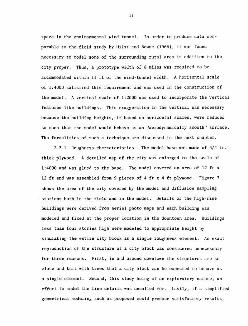
2.3.1 Roughness characteristics - The model base was made of 3/4 in.

thick plywood. A detailed map of the city was enlarged to the scale of

1:4000 and was glued to the base. The model covered an area of 12 ft x

12 ft and was assembled from 9 pieces of 4 ft x 4 ft plywood. Figure 7

shows the area of the city covered by the model and diffusion sampling

stations both in the field and in the model. Details of the high-rise

buildings were derived from aerial photo maps and each building was

modeled and fixed at the proper location in the downtown area. Buildings

less than four stories high were modeled to appropriate height by

simulating the entire city block as a single roughness element. An exact

reproduction of the structure of a city block was considered unnecessary

for three reasons. First, in and around downtown the structures are so

close and knit with trees that a city block can be expected to behave as

a single element. Second, this study being of an exploratory nature, an

effort to model the fine details was uncalled for. Lastly, if a simplified

geometrical modeling such as proposed could produce satisfactory results,

12

further development of wind-tunnel models as a tool for studying urban

diffusion would be justified.

City blocks were cut out of masonite sheets to proper proportions

and shape as dictated by the map and aerial photos. The rural area was

modeled by placing coarse sandpaper (SO Grit) and isolated patches of

higher roughness were made from coarser paper. Each of the features

were selected to contribute to the true roughness behavior of the city.

2.3.2 Heat-island effect - This feature of the prototype was

incorporated into the model by placing heat sources at the surface of the

model. Nichrome wires were laid in four different circuits over the

model as shown in Fig. 8. By changing the voltage across these circuits,

the form of the surface temperature distribution in the model city could

be controlled. Strips of fiberglass drapery cloth were placed beneath

the nichrome wires along their entire length to prevent the model surface

from being charred due to heat. The appreciable expansion experienced by

the nichrome wires during heating was taken up by providing 0.1 in. 0.0.

tensioned wire springs at the two ends of each wire. Each time the

voltage was applied to the heating wires, the model surface temperatures

were allowed to reach a steady state before data collection.

2.4 Velocity-Profile Production Technique

A number of methods were tried to produce a velocity profile over

the model similar to that in the field. The final arrangement was a grid

of cardboard tubes 2 1/2 in. diameter which were placed longitudinally at

the entrance section across the width of the tunnel in two layers. This

technique has similar advantages as those presented by Lloyd (1966) for

flat boards. Also, a 16 foot-length of the wind-tunnel floor between

13

these tubes and the model was covered with fine roughness (rice grains

glued to plywood sheets).

14

III. SIMULATION OF URBAN ATMOSPHERE AND DESIGN OF MODEL

In order that the wind-tunnel model flow corresponds to those oc­

curring in the field, it is essential that the two flows be dynamically

similar. This similarity conditions are usually sought in the differential

equations cribing motion in the prototype flow as well as in the model

flow. The conditions of dynamic similarity of a frictionless atmosphere

were first examined by Batchelor (1953). His important conclusion is that

if the flow fields are such that pressure and density everywhere depart

by small fractional smounts only from the values of an equivalent atmos­

phere in adiabatic equilibrium and if the vertical distances over which

appreciable changes in velocity occur are small compared with those for

which density variations are appreciable, the Richardson number is the

sole parameter governing dynamical similarity. Nemoto (1961 a,b,c, 1962),

Cermak et. ale (1966) and McVehil et. ale (1967) have considered a

variety of simulation problems. It is generally agreed that in case of a

thermally stratified flow of turbulent air in the surface layer, dynamical

similarity would be achieved if the model satisifes the following con­

ditions.

1. Geometrical similarity

2. Reynolds number equality

3. Richardson number equality

4. Approach flow similarity.

Effect of earth's rotation on flow in the atmospheric surface layer can

be ignored as the convective accerlation dominates the Coriolis accelera­

tion and the horizontal extent of the surface under consideration is

rather small. Cermak et.al. (1966) point out that if the prototype

lengths are less than 150 km, the Coriolis forces do not produce large

15

differences in flow patterns between model and prototype. The proposed

Fort Wayne model covers only an area of 8 x 8 miles and thus qualifies

for this simplification.

The above stated similarity criteria cannot, however, be satisfied

simultaneously between the model and the prototype. This problem is not

new in modeling practice and can be analyzed by considering the relative

importance of the different conditions in dispute. In conclusion, we

may have to resort to partial simulation when the consequences of non-

duplication of certain similarity parameters is properly understood.

The approach is that of making known and calculated approximations based

on sound knowledge.

3.1 Reynolds Number and Geometrical Similarity

Reynolds-number similarity based on the viscosity of air is neither

practical nor essential to the present modeling effort. Two alternatives

have been offered by different authors. Nemoto (196la) evolves an "eddy"

Reynolds number defined as

R e

UL = K

m

(1)

as a similarity parameter. It is obviously not a practical criterion

because the eddy diffusivities are not known off hand in the field or in

the wind tunnel. On the basis of assumptions of local isotrophy and

identity of rates of energy dissipation in the two flows, Nemoto expresses

the Reynolds number criterion for modeling wind velocity as

UocM U

cap (2)

16

This is a much more plausible form of Reynolds number similarity and has

the effect of scaling down the wind velocity instead of requiring it to

be increased for the model as was the case with ordinary Reynolds number.

The above approach to Reynolds number similarity disregards the

effects of surface terrain on flow phenomena. The fact that the turbulent

flow of air in the surface layer over an urban area is invariably

aerodynamical rough 1 opens up a new possibility. According to McVehil

et.al. (1967) an aerodynamically rough flow is similar to any other

aerodynamically rough flow irrespective of its velocity, roughness length

and kinematic viscosity. In other words, the velocity of flow, roughness

length and viscosity can be varied independently of each other. Thus if

the flow over the model is rough, the Reynolds numbers need not be equal.

On the other hand, it is essential that the surface features be suf-

fiently large and the Reynolds number sufficiently large for the model to

guarantee that the flow will have the characteristics of a flow over an

aero-dynamically rough surface.

The question whether a given surface produces an aerodynamically

fully rough flow has been discussed by Sutton (1953) and Schlichting

(1955). According to Sutton an aerodynamically rough surface is one in

which the irregularities project into the flow enough to prevent the

formation of a non-turbulent viscous layer, so that the motion is

turbulent between the roughness elements. From Nikuradse's measurements

on flow through pipes whose surfaces were uniformly covered with sand

grains of height k , the criterion for fully rough flow was determined s

to be

(3) -- ;> 75

17

where u* is the friction velocity (defined as ./TO/P , T being the o

surface shear stress and p the density of fluid) and v is the

kinematic viscosity. Nikuradsets surface roughness was so placed that a

single length such as k was sufficient to describe its properties. s

For other surfaces like the model of the city of Fort Wayne, the number

of such length parameters is increased. In addition to the height of the

city blocks, some other lengths specifying their spacing must be con-

sidered. Schlichting (1936) simplified the problem by introducing a

length called equivalent sand roughness k s

for such surfaces. He

carried out experimental determination of k for a number of roughness s

types as a function of concentration of the roughness elements. Since

then, several others have experimented with sharp edged roughness

elements (see Koloseus and Davidian 1966). Such information makes it

possible to use Nikuradse's test for roughness (as stated above) on the

city model.

Geometrical similarity between the model and the prototype is

realized if the spatial boundaries in the two bear the same ratio at the

corresponding locations. As indicated in the description of the model,

the wind-tunnel width fixes the horizontal scale of the model at 1:4000.

Now if we adopt the same ratio to scale the vertical heights in the model,

geometrical similarity will be satisfied; however, an average residential

area city block with its buildings and trees (taken to be about 25 ft

high) would scale down to 0.075 in. in the model. The concentration of

the blocks, A, is defined as the ratio of the sum of projected areas of

the blocks normal to the wind direction, to the total floor area. Rouse

(1965) and Koloseus and Davidian (1966) found, based on data from

numerous sources, that a simple relation exists between the ratio of k s

18

to actual height of roughness kl and the roughness concentration y

which is independent of the roughness shape and arrangement over the

lower range of concentration, say, below 0.1. Estimate of concentration

of blocks can be made from the map of the city. From three areas, selected

at random, a rather uniform value of 0.022 for the concentration A is

obtained if the height of the blocks is scaled to 0.075 in. From Koloseus

and Davidian (1966), equivalent sand roughness to height ratio against

It. = 0.022 is

k s -- = 2.2 mk

l

(4)

where m is an indicator of relative surface rugosity taken to be equal

to 0.88 for rectangular roughness~ With kl = 0.075 in., Eq. (4) gives

k s = 0.145 in. (5)

Using this estimate of k ,the criterion for a rough surface (Eq. 3) s

may be checked after an approximate value for u* has been established.

As is explained in the next section, Richardson-number similarity

requires the wind velocity to be as low as practicable which is opposite

to the need of keeping the flow over the model fully rough. The higher

the velocity, the greater is the temperature differential required to

produce the heat-island effect. The choice of wind velocity is thus

limited to the minimum stable value attainable with the existing wind-

tunnel propeller system. This velocity is 8 ft/sec and is used to

evaluate the similarity criteria.

If the boundary layer over a flat plate is turbulent from the leading

edge, the local skin-friction coefficient cf is given by Schlichting

(,1955) as

19

2 u* 1 U2 = 2 c t

f 00

5 x 105 <

=

R x

0.0296 (R)- 1/5 x

< 107 (6)

where R U x and is distance from the leading edge. If the model = ()() x x

v is placed 20 ft from

= 0.345 ft/sec.

the leading edge, R x

Using this value and

14k s v =

= lOG

k s

and from Eq. (6) ,

from Eq. (5), we get

26.1 < 75 (7)

According to Nikuradse's criterion given by Eq. (3), flow over a model

scaled by 1:4000 vertically and horizontally is not aerodynamically rough.

There are only two alternatives available to improve upon the

magnitude of to ensure that the flow is fully rough. One is to v

augment u* by increasing the wind velocity over the model and the

other is to increase k s The former tends to make similarity of the

heat-island effect impracticable and has to be discarded as a means of

rectifying the situation. We are, thus, left with only one choice viz.,

to exaggerate the vertical scale of the model. The distorted models are

not uncommon in hydraulics and ocean engineering laboratory studies.

This compromise between geometrical and Reynolds number similarity is

not expected to introduce any serious limitation if a fully rough flow

is produced in the wind tunnel. Some encouragement for distorted models

comes from the equations of motion of a turbulent atmosphere as brought

out by Nemoto (1961). The degree of vertical exaggeration is related

to ISc and K , the turbulent diffusivities in the longitudinal and z

vertical directions respectively, as

[K K '] _ 2E. zM 1/2

(l - K . K xM zp·

(8)

20

where subscripts M and p stand for model and prototype. In the wind

tunnel K and K are expected to be of the same order whereas in the x z

field Kx is at least one order of magnitude bigger than K z (see for

example, Kao and Wendell 1968 and Orgill 1970). Thus a vertical ex­

aggeration a = /DO ~ 3 is permissible in modeling atmospheric flow.

Let us consider a vertical exaggeration of the model by a factor of

2 which, by definition, doubles the concentration of the city block.

From Koloseus and Davidian (1966)

number is

k = 0.58 in. and surface Reynolds s

= 104 > 75 (9)

Thus Nikuradse's criterion is satisfied and the flow over the model is

fully rough aerodynamically if a vertical scale 1:2000 is used.

3.2 Richardson Number Similarity

In order to model the heat-island effect, the bulk Richardson

numbers must be equal for model and prototype. It is defined as

gL ~T = 0 (10)

U~ Ta

where the subscript '0' denotes the value of a quantity with respect to

a reference height. Thus, U is the velocity at the reference height o

and ~T is the temperature difference between the surface and the ref­o

erence height, T denotes the average temperature, a L the character-

istic length of flow and g the gravitational acceleration. In this

study, the entire thermal structure is considered to be developed by

heat sources within the city; therefore, elevated inversions and lapses

in the upstream flow are eliminated from consideration. The thermal

21

structure over the model and the prototype will be similar if

[gL£\T ~1

U2 T 1M o a

= [

gL£\Tol

u2 T Jp o a

To start with, it is reasonable to assume that (Ta)M' the average

temperature in the model is the same as that for the prototype (Ta)p'

then the condition of similarity is

In order to evaluate the temperature differential over the model

we shall consider the specific field tri~l intended to be modeled. Of

the six "reliabletl trials analyzed by Csanady, Hilst and Bowne (1967),

half are designated as stable and half as moderately stable. As the

(11)

(12)

present study is limited to the consideration of a neutral approach flow,

one of the near-neutral trial 6S-06-G2 is selected for modeling. For

simulating the vertical heat-island effect, a reference height equal to

100 ft is selected. From G.T. Tower temperature data, the temperature

differential £\T is found to be about 0.28oC. The ratio U op ( oM) may

U U be approximated by ( ~1) since the velocity profile in the op wind

UOO

tunnel is also to be R maoe similar to that in the field. For the trial

under consideration, velocity at about 3000 ft in the field is on the

average 26 ft/sec and can be taken to be comparable to the proposed wind-

tunnel air speed of 8 ft/sec. Thus, the temperature differential in the

wind tunnel is given by Eq. (12) as,

~ ToM = 0.28 (2000) (2~)2 °c

= 53.2oC ~ 960 F (13)

22

Thus, the Richardson number over the model will be similar to that over

Fort Wayne within the first 100 ft at the G.T. Tower if a temperature

differential of about 1000F is maintained in the model at the corresponding

position.

If the surface of the model is to be heated by resistance filaments

(nichrome wire), it is necessary to investigate the feasibility of this

scheme. This can be done by evaluating the power needed to huat the

model in order to maintain the design temperature differential over it.

We shall, thus, have to consider the heat transfer from the model in all

the three modes--convection , conduction and radiation.

1. Forced Convection~-There will be a spatial distribution of

temperature over the model and the total temperature differential between

the surface air and the free stream may be in excess of 1000P. On the

average, however, we may assume that the surface is maintained, say, at

l500p above the ambient temperature (of, say, 600p). The average heat-

transfer coefficient, h , over a rough plate under forced convection is c

(see for example, Krieth 1967),

[u L]O.S

he= 0.037 .: ~ (Pr)0.33 (14)

where k and Pr are the thermal conductivity and Prandtl number for

air, L is the length of heated surface which is about 6 ft in the model,

and Uw is the freestream velocity 8 ft/sec. If the fluid properties

are evaluated at

1 0 Tf = -2 (T f + T ) = 135 P sur ace 00 (15)

Eq. (14) gives Accordingly, the heat transfer

from the model (area ~ 36 ft 2 ) due to forced convection is

23

q1· = h (T f - T ) x model area c sur ace 00

= 1.8 (150) x 36 ~ 9,700 Btu/hr (16)

2. Conduction--If there is a Ii in. thick layer of plywood between

the heated surface and the bottom of the wind-tunnel floor which may be

at near-ambient temperature, some of the heat will be conducted through

the plywood and lost by convection through the room. Taking thermal

conductivity k of plywood as 0.1 Btu/hr ft of and floor temperature

of, say, 100oF, heat transfer due to conduction through the wind tunnel

floor is

A k U -T ) q2 = t surface floor plywood

36xO.l (110) = 1.5/12 ~ 3,200 Btu/hr (17)

3. Radiation--The model is nearly completely surrounded by the

wind tunnel on one side such that the geometry factor, G , may be

taken to be 0.5. The net rate of heat transfer is given by

q3 = o£AG (T· 4d 1 - TW'4T 11) mo e . . wa s (18)

where 0 is the Stefan-Boltzmann constant with a value of 0.17lxlO-s

Btu/sq ft °R4 and is the emissivity of a plywood surface and Tt

is the absolute temperature in degrees Rankine. Upon substitution of

the relevant data, the heat transfer due to radiation is

~ 4,100 Btu/hr (19)

24

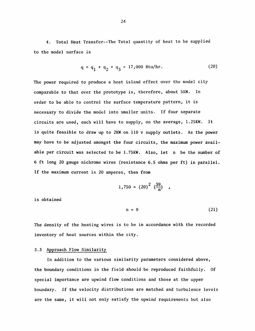
4. Total Heat Transfer--The Total quantity of heat to be supplied

to the model surface is

q = ql + q2 + q3 = 17,000 Btu/hr.

The power required to produce a heat island effect over the model city

comparable to that over the prototype is, therefore, about 5KW. In

order to be able to control the surface temperature pattern, it is

necessary to divide the model into smaller units. If four separate

(20)

circuits are used, each will have to supply, on the average, 1.25KW. It

is quite feasible to draw up to 2KW on 110 v supply outlets. As the power

may have to be adjusted amongst the four circuits, the maximum power avail-

able per circuit was selected to be 1.75KW. Also, let n be the number of

6 ft long 20 gauge nichrome wires (resistance 6.5 ohms per ft) in parallel.

If the maximum current is 20 amperes, then from

is obtained

1,750 = (20)2 (39) n

n = 9 (21)

The density of the heating wires is to be in accordance with the recorded

inventory of heat sources within the city.

3.3 Approach Flow Similarity

In addition to the various similarity parameters considered above,

the boundary conditions in the field should be reproduced faithfully. Of

special importance are upwind flow conditions and those at the upper

boundary. If the velocity distributions are matched and turbulence levels

are the same, it will not only satisfy the upwind requirements but also

25

take care of the boundary-layer thickness over the model. Moreover, the

longitudinal pressure gradient in the ambient flow over the model should

be adjusted zero as is the case in the field.

3.4 Diffusion Similarity

Once the similarity of flow is established, similarity in diffusion

characteristics will follow if the linear dimensions of the source

configuration are scaled properly. For example, the height of the quasi­

instantaneous source in the wind tunnel should correspond to the best

estimates of the airp1ance elevation. Csanady et.a1. (1969) fix the

cloud height at 75m for the trial 65-06-G2 which scales down to 1.48 in.

in the model. Also the speed of the tracer release air craft is scaled

to about 4 ft/min. One aspect of the field release method which cannot

be readily simulated is the initial dispersion of the cloud in the wake

of the air craft. This inability to model the initial conditions of the

diffusion phenomena should not seriously affect similarity of distribution

of the tracer material at distance downwind extending 10 - 20 times the

source height.

26

IV. EXPERIMENTAL RESULTS AND DISCUSSION

In this chapter are presented the results of the measurements per­

formed on the model of the city of Fort Wayne in the environmental wind

tunnel at the Fluid Dynamics and Diffusion Laboratory of Colorado State

University_ The performance of the model in reproducing field flow

characteristics is discussed. The model results are compared with those

of the field trial 65-06-G2 (which was specifically modelled) and theory.

Results of some visualization experiments, which were conducted before

intensive model testing, are also presented.

4.1 Data

Model data were based on the values of test variables selected in

the chapter on model design. Some of the data, which could not be pre­

sented wholly in graphical form, is arranged in tablular form in Appendix

A. This is mostly the surface-dosage data obtained with and without

incorporating the heat-island effect in the city model. All the vertical

distributions are given only in graphical form. These include vertical

temperature, velocity, turbulence and dosage data.

4.2 Approach Flow

The flow approaching the city area is characterized mainly by

velocity and turbulence distribution in the vertical~ For the velocity

profile reproduction, tower data (G.T.) and balloon data (Site 2) formed

a set which could be compared directly to wind-tunnel velocity data at

the corresponding location. After many trials, the two profiles were

matched as shown in Fig. 9. Although turbulence data are sparse in the

field, a comparison of whatever data are available is essential from the

point of view of assessing model behavior. Figure 10 shows the vertical

27

distribution of longitudinal turbulence intensity in the wind tunnel

along with field data. The agreement between the field and wind tunnel

velocity and turbulence intensity profiles approaching the city provides

much encouragement for arriving at a satisfactory simulation of flow

and diffusion near the city.

4.3 Flow Over the Model City

The model city modifies the approaching flow both in respect to

velocity and temperature characteristics. Figure 11 shows the velocity

distributions at WANE T.V., G.T. Tower and mid-city locations. Whereas

the WANE and G.T. profiles are nearly alike, that over the mid-city

differs considerably and the joint effect of roughness and heating ex­

tends to a height equivalent to 200 meters in the prototype. Longitudinal

turbulence intensity at the city block top level registers an increase

from 29% at WANE to 42% at G.T. near the downtown area as shown in Fig.

12. The effect of the roughness on turbulence intensity is more pro­

nounced than that on mean velocity and has already reached about the 75

meter level at G.T. Figure 13 shows the development of vertical temper­

ature profiles over the model. The location of vertical temperature

profile stations is indicated on the surface temperature map. The shape

of the heat island produced in the wind tunnel is depicted in Fig. 14

and is based on surface temperature data gathered at SO locations. Al­

though field data for the trial 6s-06-G2 is available only at 10 locations,

the rough picture of the heat island that emerges from them (Fig. IS) is

remarkably similar to that obtained in the wind tunnel as shown in Fig.

14. This likeness in the heat-island shapes may be regarded as an

evidence of the right interaction between the model geometry and the

proper distribution of heat sources. Thus, flow over the city of Fort

28

Wayne is modelled well when the bulk Richardson numbers for model and

prototype are equal at the city center.

4.4 Visual Observations

The dispersion of smoke plumes released at ground level upwind from

the city was studied visually to observe if any spurious circulation

patterns were present. The flow was found to be generally well behaved.

In Fig. 16 are presented pictures of a smoke plume released at the start

of the model upwind from WANE T.V. Tower. It is noticed that the plume

experiences a sudden increase in its vertical spread as it passes over

the city proper. Also, the lateral movement at the surface is seen to be

along the streets. All this agrees generally with the field experience.

4.5 Diffusion Results and Comparison with the Field Data

The model diffusion results are first compared with the field data

and then with the theory. All the dosage data is reduced to non-dimen-

sional form for these comparisons by writing the non-dimensional dosage

D as

ID (22)

where D is the observed dosage, Uh the wind velocity at the source

height hand Q the source strength. Model quantities were control-

led and were, thus, known precisely. There is, however, some uncertainty

regarding hand Q values in the field. The adjusted figures for

these parameters as given by Csanady et.al. (1967) are used in pre-

ference to those based on air-craft data.

The surface dosage measurements, made at 250 stations on the model,

are presented in Fig. 17 in the form of iso-dosage lines. These iso-lines

are based on five station dosage averages to smooth the variability of

29

the individual dosages and to highlight the general characteristics.

The highest non-dimensional dosage occurs in the rural area and has a

value of 0.36. Also the area covered by a dosage equivalent to the city

maximum is much larger in the rural area then it is in the city.

A closed contour downwind from the downtown area can be attributed

to mixing by the high-rise buildings which help to diffuse the higher

concentration in the core of the plume to ground level. The lines up to

1 1/2 ft from the walls are obliterated as the end effects due to the

finite length of the line source become important in this region. The

iso-dosage lines are fairly parallel upwind from the city and far in the

rural area (say, 5 miles from mid-city) beside it. Thus the effect of

the city extends in the cross-wind direction up to about half the city

width from the outskirts beyond which the two dimensionality of the flow

and the line source diffusion remains intact.

A similar plot of iso-dosage lines from field data (based on five

station averages) is shown in Fig. 18. No systematic conclusions can

be drawn from these data as the dispersion over the city area does not

distinguish itself as clearly from that over the rural area. A better

picture of surface dosage distributions over these areas is obtained

from Fig. 19 reproduced from Hilst and Bowne (1966). This represents

an average of all the 70 field trials and is in qualitative agreement

with the model pattern. A comparison of the non-dimensional surface

dosages obtained in the model experiments and the field trial 65-06-G2

at the fourth sampling line is made in Fig. 20. The two lateral dosage

distributions show remarkable similarity in exhibiting the effect of the

city on the dispersion process. Both show a dip of nearly the same shape

in the dosage variation downwind from the city. Ten station average

30

dosages, plotted in the same figure further illustrate the effect of the

city. The field dosages, however, show much more variability than the

model data.

The longitudinal variation of ground dosages in the model city and

the prototype are presented in Fig. 21. Also imposed on the oraph is a

similar relationship for the model but without the heat-island effect.

The ground-level dosage in the field rises much more rapidly with dis-

tance than that in the model and starts decreasing from the first

sampling line downwind. This is rather a sudden fall of the tracer

material to the ground and takes place upwind of the city. Csanady

et.al. (1967) explained it to be due to turbulence generated by the

rural area (indicating a roughness length

Hanna (1970) shows a value of 15 cm for

z o = 3M). Analysis by

z which seems more appropriate o

index of roughness over farmlands. It appears that the initial disper-

sion of the tracer in the wake behind the air-craft which could not be

reproduced in the laboratory might have been responsible for transporting

the material to the ground earlier than would be caused by rural area

turbulence alone. The effect of the downdraft from the disseminating

air craft in causing substantial increase in ground-level dosages has

been recognized by Vaughan and McMullen (1963) and Vaughan (1965). In

such circumstances, direct comparison with the field data is not possible

near the source. Away from the release line, the model and prototype

data indicate nearly the same rate of decrease of dosage with distance

and is indicated more clearly in Fig. 22. This comparison is very

significant in that the rate of decrease of dosage represents the total

effect of the city (both roughness and heat island). Moreover, the two

cases become equivalent, despite the downdraft anomaly, at large

31

distances from the source as the tracer tends to "forget" its initial

position. Thus the model gives a better overall picture of the effect

of the city on dispersion process by excluding the aircraft downdraft

effect in the field tests. The comparison of the model curves for

dosage variation with and without the inclusion of the heat island

effects in the city, clearly shows the importance of the internal heating

upon the dispersion over a city. The maximum dosage in the city due to

an elevated source would be reduced if the heat island is not present

but the rate of decrease of dosage would be much slower. In general,

elevated releases over an urban complex cause greater ground-level

dosages than similar releases over a flat terrain. This effect emphasizes

the need for locating industrial plants with tall stacks away from the

cities.

Some idea of the growth of plumes in the field and the model can be

obtained by computing a z

ground dosage is related

from Sutton's model.

a z as

D o = /!.. h

1f a z

The non-dimensional

(23)

For a given value of Do' ~ and hence az can be obtained from Eq. (23). a z

Figure 23 shows a comparison of field and wind-tunnel rates of growth of

the cloud vertically. The two sets of data match reasonably well away

from the source.

4.6 Comparison with Theory

Presently there is no theory of diffusion of a passive substance

which incorporates surface roughness inhomogeneity and the heat-island

effect. However, it is of practical importance to investigate the

32

possibility of using theoretical results based on the assumption of

horizontal homogeneity. This can be done by using the local value of

variable flow characteristics like shear velocity, roughness length

determined from the flow field at the position of interest. The com-

parison between wind-tunnel data and theoretical results will be limited

to Smith's (1957) model. According to this model, the velocity and

vertical diffusivity are assumed to be distributed as follows:

and

~h = [{r

K z

~ [

zll-a = hj

(24)

(25)

(~ is the vertical diffusivity at source height, h). The solution of

the two-dimensional diffusion equation for non-dimensional dosage ID

is then given by

I

where Q = source strength (~ci/cm),

D = mean dosage (~ci-min/cc),

z Z;; = h = non-dimensional height, and

2Z;; (l+2a)/2l (l+2a)2~ ~

non-dimensional longitudinal distance,

I = Modified Bessel function of the first order.

(26)

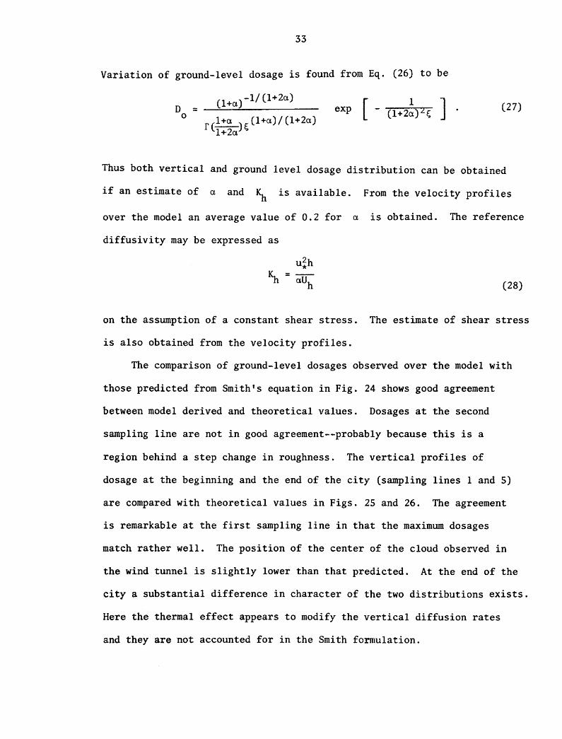
33

Variation of ground-level dosage is found from Eq. (26) to be

( l+a) -1/ (l+2a) D = --~~~------------

o rcl +a )~(1+a)/(l+2a) l+2a

exp (27)

Thus both vertical and ground level dosage distribution can be obtained

if an estimate of a and ~ is available. From the velocity profiles

over the model an average value of 0.2 for a is obtained. The reference

diffusivity may be expressed as

(28)

on the assumption of a constant shear stress. The estimate of shear stress

is also obtained from the velocity profiles.

The comparison of ground-level dosages observed over the model with

those predicted from Smith's equation in Fig. 24 shows good agreement

between model derived and theoretical values. Dosages at the second

sampling line are not in good agreement--probably because this is a

region behind a step change in roughness. The vertical profiles of

dosage at the beginning and the end of the city (sampling lines land 5)

are compared with theoretical values in Figs. 2S and 26. The agreement

is remarkable at the first sampling line in that the maximum dosages

match rather well. The position of the center of the cloud observed in

the wind tunnel is slightly lower than that predicted. At the end of the

city a substantial difference in character of the two distributions exists.

Here the thermal effect appears to modify the vertical diffusion rates

and they are not accounted for in the Smith formulation.

34

v. CONCLUSIONS

The possibility of modeling urban atmospheres and diffusion was

explored by reproducing characteristics of flow over the city of Fort

Wayne, Indiana in a wind tunnel. The dynamic similarity between wind

tunnel and natural full~scale flows was achieved by designing the model

such that flow over it was fully rough in an aerodynamic sense and the

Richardson numbers were the same. The condition of fully rough flow

was considered more crucial than strict geometrical similarity which was

compromised for by exaggerating the vertical scale. In addition, the

approach flow in the model was made to be similar to the atmospheric

boundary layer.

The heat-island pattern in the wind tunnel was found to be similar

to that in the field, which is good evidence that the model geometry and

heat-source distribution interacted in a similar manner in the two cases.

The surface-dosage measurements lead to the same general conclusions as

the field data. The highest dosages occur in the rural area. The high­

rise buildings tend to cause a local region of high dosages. The effect

of the city extends in the cross-wind direction up to about half the city

width from the outskirts beyond which the two dimensionality of flow

remains intact. The rate of decrease of dosage at street level, far

from the source, follows the same trend for model and full-scale data.

The vertical and ground-level dosage distribution compares well with

Smith's (1957) analysis.

A method of dosage determination is evolved for analyzing quasi­

instantaneous source diffusion. Also the method of heating the model

surface with nichrome-wire heating elements offers great versatility in

producing thermal stratifications in the wind tunnel.

35

The present study did not include effects from undulation of the

terrain and the approach flow was considered neutral. Furthermore, no

attempt was made to model the climatic variation other than wind and

temperature. The agreement found in flow and diffusion data for the

model and the full-scale natural flow indicate that these complicating

features can be studied by means of physical modeling.

The results of this study have proved that it is possible, at least

for neutral approach flows, to simulate the flow over complex surface

such as a city and obtain useful information, relatively inexpensively,

on urban diffusion. This investigation opens the way for studies of

air-pollution problems for purposes of urban planning. The location of

industrial sites and power-generation complexes relative to major

topographical features, the location of freeways through existing cities,

the grouping of tall buildings in an urban-development program, or the

location of an entirely new city relative to topographic features to

minimize air pollution potentials under adverse meteorological conditions

can be studied systematically.

36

REFERENCES

Batchelor, G. K. (1953), "The Conditions for Dynamical Similarity of Motions of Frictionless Perfect-Gas Atmosphere." Quarterly Journal of Royal Meteorological Society, Vol. 79, pp. 224-235.

Cermak, J. E., Sandborn, V. A., Plate, E. J., Binder, G. H. Cnuang, H., Meroney, R. N., and Ito, S. (1966), "Simulation of Atmospheric Motion by Wind Tunnel Flows," Fluid Dynamics and Diffusion Laboratory Report CER66-l7, Colorado State University.

Corrsin, S. (1949), "Extended Applications of the Hot-Wire Anemometer," NACA Tech. Note 1864.

Csanady, G. T., Hilst, G. R., and N. E. Bowne (1967), "Turbulent Dif­fusion From a Cross-Wind Line Source in Shear Flow at Fort Wayne, Indiana," Atmospheric Environment, Permagon Press, Vol. 1, pp. 79-99.

Davis, M. L. (1968), "Modeling Urban Atmospheric Temperature Profiles," Ph.D. Dissertation, Department of Civil Engineering, University of Illinois, Urbana, Illinois.

Hanna, S. R. (1970), "Turbulence and Diffusion in The Atmospheric Boundary Layer Over Urban Areas," Seminar presented at Syracuse U., Feb. 1970.

Hilst, G. R., and Bowne, N. E. (1966), "A Study of the Diffusion of Aerosols Released from Aerial Line Sources Upwind of an Urban Complex." Final Report, Contract No. DA42-007-AMC-38(R), to Dugway Proving Ground. The Travelers Research Center, Inc., Hartford, Conn.

Kao, S. K., and Wendell, L. K. (1968), "Some Characteristics of Relative Particle Dispersion in the Atmosphere's Boundary Layer," Atmospheric Environment, Pergamon Press, Vol. 2, pp. 397-407.

Koloseus, H. J., and Davidian, J. (1966), "Roughness-Concentration Effects on Flow Over Hydrodynamically Rough Surfaces," U.S. Geological Survey Water-Supply Paper l592-C, D.

Kovasnay, L. S. G. (1953), "Turbulence in Supersonic Flow," Journal of Aeronautical Sciences, Vol. 20, pp. 657-674.

Kreith, F. (1962), "Principles of Heat Transfer," International Text Book Co., Scranton, Penn.

Lloyd, A. (1966), "The Generation of Shear Flow in a Wind Tunnel," Quarterly Journal of Royal Meteorology, Vol. 93, pp. 79-96.

McVehil, G. E., Ludwig, G. R., and Sundaram, T. R. (1969), "On the Feasibility of Modeling Small Scale Atmospheric Motions," Cornell Aeronautical Laboratory, Inc., CAL Report No. 2B-2328 P-l.

37

Myrup, L. O. (1969), itA Numerical Model of the Urban Heat Island," Journal of Applied Meteorology, Vol. 8, pp. 908-918.

Nemoto, S. (196la), "Similarity Between Natural Wind in the Atmosphere and Model Wind in a Wind Tunnel (I)," Papers in Meteorology and Geophysics, Vol. 12, No.1, pp. 30-52.

Nemoto, S. (196lb), "Similarity Between Natural Wind in the Atmosphere and Model Wind in a Wind Tunnel (II)," Papers in Meteorology and Geophysics Vol. 12, No.2, pp. 117-128.

Nemoto, S. (196lc), "Similarity Between Natural Wind in the Atmosphere and ~fodel Wind in a Wind Tunnel (III), II Papers in Meteorology and Geo­physics, Vol. 12, No.2, pp. 129-154.

Nemoto, S. (1962), "Similarity Between Natural Wind in the Atmosphere and Model Wind in a Wind Tunnel (IV)," Papers in Meteorology and Geophysics, Vol. 13, No.2, pp. 171-195.

Orgill, M. M. (1970), Personal Communication on Magnitude of Diffusivities.

Rouse, H. (1965), "Critical Analysis of Open Channel Resistance," Pro­ceedings of the American Society of Civil Engineers, Journal of the Hydraulics Division, Paper 4387.

Schlichting, H. (1936), "Experimentelle Untersuchungen zun Rauhigkeit's Problem," Ingenieur-Archiv., Vol. 7, No.1, pp. 1-34 [Translation, NACA Tech. Memo, 823, April 1937].

Schlichting, H. (1960), ttBoundary Layer Theory," Fourth Edition, McGraw­Hill, New York.

Smith, F. B. (1959), "The Diffusion of Smoke from a Continuous Elevated Point Source into a Turbulent Atmosphere," Journal of Fluid Mechanics, Vol. 2, pp. 49-76.

Sutton, O. G. (1953), "Micrometeorology," McGraw-Hill, New York.

Turner, D. B. (1964), "A Diffusion Model for an Urban Area," Journal of Applied Meteorology, Vol. 3.

Vaughan, L. M. (1965), "Further Analysis of Intermediate-Scale Aerosol Cloud Travel and Diffusion Data from a Low-Level Aerial Line Releases," Technical Report No. 117, Aerosol Laboratory, Metronics Associates, Inc., Pala Alto, California.

Vaughan, L. M., and McMullen, R. W. (1963), "Intermediate Scale Aerosol Cloud Travel and Diffusion from Low-Level Aerial Line Releases," Technical Report No. 97, Aerosol Laboratory, Metronics Associates, Inc., Pala Alto, California.

38

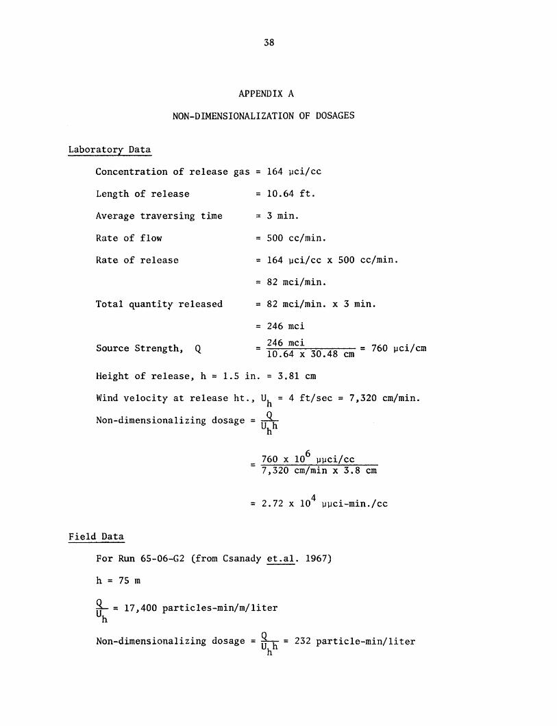
APPENDIX A

NON-DIMENSIONALIZATION OF DOSAGES

Laboratory Data

Concentration of release gas = 164 pei/ee

Length of release = 10.64 ft.

Average traversing time = 3 min.

Rate of flow = 500 ee/min.

Rate of release = 164 pei/ee x 500 ee/min.

= 82 mei/min.

Total quantity released = 82 mei/min. x 3 min.

= 246 mei

246 mei 760 }.lei/em = = 10.64 x 30.48 em Source Strength, Q

Height of release, h = 1.5 in. = 3.81 em

Wind velocity at release ht., Uh = 4 ft/see = 7,320 em/min.

Non-dimensiona1izing dosage = ~ Uhh

760 x 106 ppei/ee = =-~~--~~~=-~--7,320 em/min x 3.8 em

= 2.72 x 104 ppci-min./ce

Field Data

For Run 65-06-G2 (from Csanady et.a1. 1967)

h = 75 m

&- = 17,400 partic1es-min/m/1iter h

Non-dimensiona1izing dosage = ~ = 232 particle-min/liter Uhh

39

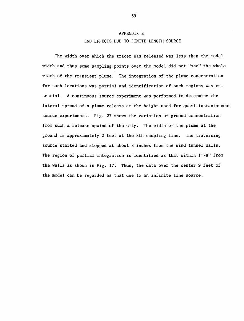
APPENDIX B

END EFFECTS DUE TO FINITE LENGTH SOURCE

The width over which the tracer was released was less than the model

width and thus some sampling points over the model did not "see" the whole

width of the transient plume. The integration of the plume concentration

for such locations was partial and identification of such regions was es­

sential. A continuous source experiment was performed to determine the

lateral spread of a plume release at the height used for quasi-instantaneous

source experiments. Fig. 27 shows the variation of ground concentration

from such a release upwind of the city. The width of the plume at the

ground is approximately 2 feet at the 5th sampling line. The traversing

source started and stopped at about 8 inches from the wind tunnel walls.

The region of partial integration is identified as that within 1'-8" from

the walls as shown in Fig. 17. Thus, the data over the center 9 feet of

the model can be regarded as that due to an infinite line source.

40

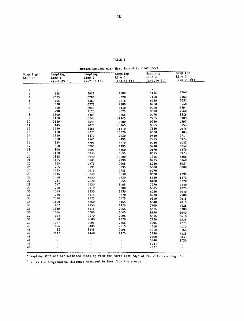
TABLE

Surface Dosages ~ith Heat Island l ~~c i-mini ee)

SampUng* Sampling Sampling Sampling Sampling SalllpIill~

Station Line 1 Line 2 Line 3 Line -l Line :;

+(x-1.03 ft) (x=2.87 ft) (x=4.33 ft) (x=6,16 ft) lx=S.llll ft)

1 Sib9 2 535 2915 4880 4125

3 2325 678S 9320 7150 730~

4 555 7360 9575 6940 7032 5 530 6775 7500 8950 b53S 6 520 8945 8440 9950 5494 7 790 7170 9075 9090 -l5uO 8 1300 7485 9765 9050 53':!:> 9 1170 6240 11445 7725 5989

10 1140 7345 9700 9730 6593 11 445 7025 10765 8005 uI5:; 12 1230 5365 11410 7530 6U4S 13 470 9320 10270 6650 b483 14 1320 8470 9930 9410 5714 15 620 7545 8495 7975 b923 16 33t; 8795 8770 9040 6043 17 650 6980 7495 10210 5054 18 800 7095 8360 9170 5879 19 1420 69.30 6655 8675 6923' 20 1115 bb40 105()0 7715 6868 21 1185 bIS5 7990 8275 6868 22 565 6875 7465 8280 5934 23 765 595 9095 6500 5000 24 1335 9515 7585 6970 25 1615 10840 8<>30 8670 4395 26 1460 8680 9120 8540 1373 27 711 7220 9555 8400 5770 28 787 9150 I10b5 7970 5840 29 200 9110 9380 6585 4875 30 1395 9450 5430 6050 50-l0 31 749 8115 9370 6230 7580 32 2320 8925 7975 6610 7615 33 1509 6360 6155 6640 7015 34 467 7550 7725 7400 6525 35 1319 8115 7055 6325 5780 36 1026 6200 7645 9150 5040 37 924 7270 7095 8815 5610 38 1390 8600 7320 7720 5525 39 1047 9095 7865 5295 4275 40 656 9485 7615 4910 4':10 41 412 5145 7095 4720 5165 42 2112 1440 4475 5740 5825 43 b400 5835 44 5940 5730 45 52·U 46 4532

* Samp 1 ing stations are numbereo starting from the north cast eoge of the city lst.'c Fig. :-1. + is the longitudinal distance measured in feet from the source. x

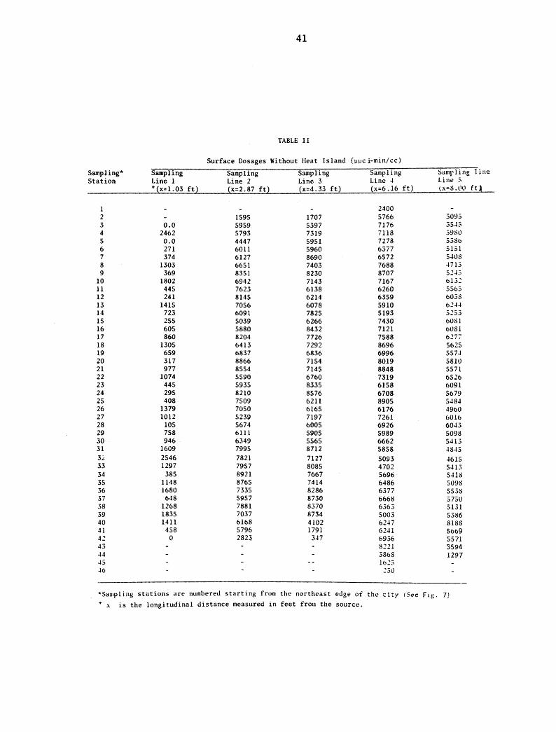
41

TABLE II

Surface Dosages Without Heat Island (uuc i-min/eel

Sampling* Sampling Sampling Sampling Sampling Sampling 1ine Station Line 1 Line 2 Line 3 Line .t Line 5

+ (x=1.03 ft) (x=2.87 ft) (x=4.33 ft) (x=6.16 ft) lx=S.LlLl ftA

1 2400 2 1595 1707 5766 3095 3 0.0 5959 5397 7176 .35.t5 4 2462 5793 7319 7118 3980 5 0.0 4447 5951 7278 53S<> 6 271 6011 5960 6377 5151 7 374 6127 8690 6572 5.t08 8 1303 6651 7403 7688 .t713 9 369 8351 8230 8707 52.t5

10 1802 6942 7143 7167 01.32 11 445 7623 6138 6260 5505 12 241 8145 6214 6359 6038 13 1415 7056 6078 5910 02.t.t 14 723 6091 7825 5193 5253 15 255 5039 6266 7430 60S1 16 605 5880 8432 7121 6081 17 860 8204 7726 7588 6277 18 1305 6413 7292 8696 5625 19 659 6837 6836 6996 557.t 20 317 8866 7154 8019 5810 21 977 8554 7145 8848 5571 22 1074 5590 6760 7319 6526 23 445 5935 8335 6158 6091 24 295 8210 8576 6708 5679 25 408 7509 6211 8905 5484 26 1379 7050 6165 6176 4900 27 1012 5239 7197 7261 6010 28 105 5674 6005 6926 604.3 29 758 6111 5905 5989 5098 30 946 6349 5565 6662 5413 31 1609 7995 8712 5858 .t845 3';: 2546 7821 7127 5093 4615 33 1297 7957 8085 4702 5-113 34 385 8921 7667 5696 5-118 35 1148 8765 7414 6486 5098 36 1680 7335 8286 6377 5538 37 648 5957 8730 6668 5750 38 1268 7881 8370 636.3 5131 39 1835 7037 8734 5003 5386 40 1411 6168 4102 6247 8188 41 458 5796 1791 6241 6609 42 0 282.') 347 6936 5571 43 8221 5594 44 .>8oS 1297 45 Ib25 46 230

*Salllpi ing stations are numbered starting from the northeast edge of the ~ity (S~e Fig. 7) + x is the longitudinal distance measured in feet from the source.

42

TABLE III

ELEVATED FIXED SOURCE CONCENTRATIONS AT GROU~O LEVEL

WITU HEAT ISLANO

Sampling *y Line (in)

1 +4.5 +(x=I.03 ftl +2~S

+1.5 +0.5 -0.5 -1.0 -1.5 -2.0 -2.5 -4.0

3 +12.0 (x=4.33 ft) +9.0

+6.0 +4.0 +3.0 +2.0 +1.0

0 -1.0 -3.0 -5.0 -6.5 -9.S

Concentration ()Juci/cc)

2 19 96

230 247 193 102

71 38 0

0 15 69

234 431 520 576 758 843 663 331 62 10

*y is the model distance measured Positive towards north

Q = 1550 IAci/min

Sampling Y Concentration Sampling Line (in) (1JIJci/cc) Line

7A +7.0 0 2 (x=1.95 ft) +5.0 32 (x=l.87 ft)

+3.0 161 +2.0 478 +1.0 905

0 922 -1.0 1011 -2.0 685 -2.5 365 -4.25 106 -5.25 23 -7.25 7 -9.25 0

4 +12.0 0 5 (x=6.1t> ft) +9.0 0 (x=S.OO ft)

+5.0 85 +3.0 240 +1.0 400

0 457 -1.0 461 -2.0 451 -3.0 321 -4.0 148 -6.0 29 -9.0 12 -12.0 0

in inches from the centreline of the plume.

+ x is the longitudinal distance measured in feet from the source.

Y Con..::cntrati..>11 (in) te~d!~d

+8.0 0 +7.0 0 +5.0 90 +3.0 .. 50 +2.0 767 +1.0 907

0 890 -1.0 910 -2.0 799 -4.0 .335 -6.0 35 -S.O 22

+12.0 18 +9.0 84 +6.0 180 +4.5 247 +3.0 289 +1.5 301

0 279 -1.0 321 -3.0 225 -6.0 130 -9.0 41 -12.0 6

43

TABLE IV

SURFACE AIR TEMPERATURES OVER THE ~1ODEL

Sampling *y' Temp. Sampling y' Temp. Sampling Y' rl..'mp. Line (in) ( OF) Line (in) (oF) Line (in) \. oF)

28 77.5 2 16 60.0 3 13 57.5 ... (x:;::!. 03 ft) 40 100.5 (x=2.87 ft) 28 61.0 (x=4.33 ft) 25 58.0

52 77.5 40 62.0 37 65.5 64 95.0 52 83.5 51 156.5 76 91.5 77 210.5 67 1.19.0 88 135.5 98 201.5 79 118.0

100 164.5 111 148.0 92 132.3 112 103.0 131 176.0 107 158.5 124 66.5 143 58.0 119 123.5 139 60.5 127 120.0

4 19 57.5 5 16 56.0 (x=6.16 ft) 31 58.2 (x=8.00 ft) 40 57.0

43 61.0 55 66.5 55 73.0 67 62.5 67 72.6 79 78.0 79 172.0 91 88.5 91 215.0 103 68.2

100 104.5 116 66.4 112 70.3 124 63.2 121 70.0

+x is the longitudinal distance measured in feet from the line source.

*y' is the distance measured in inches from the northeast edge of the model.

44

ENVIRONMENTAL WIND TlNVEL

Figure 1. Environmental Wind Tunnel

'-

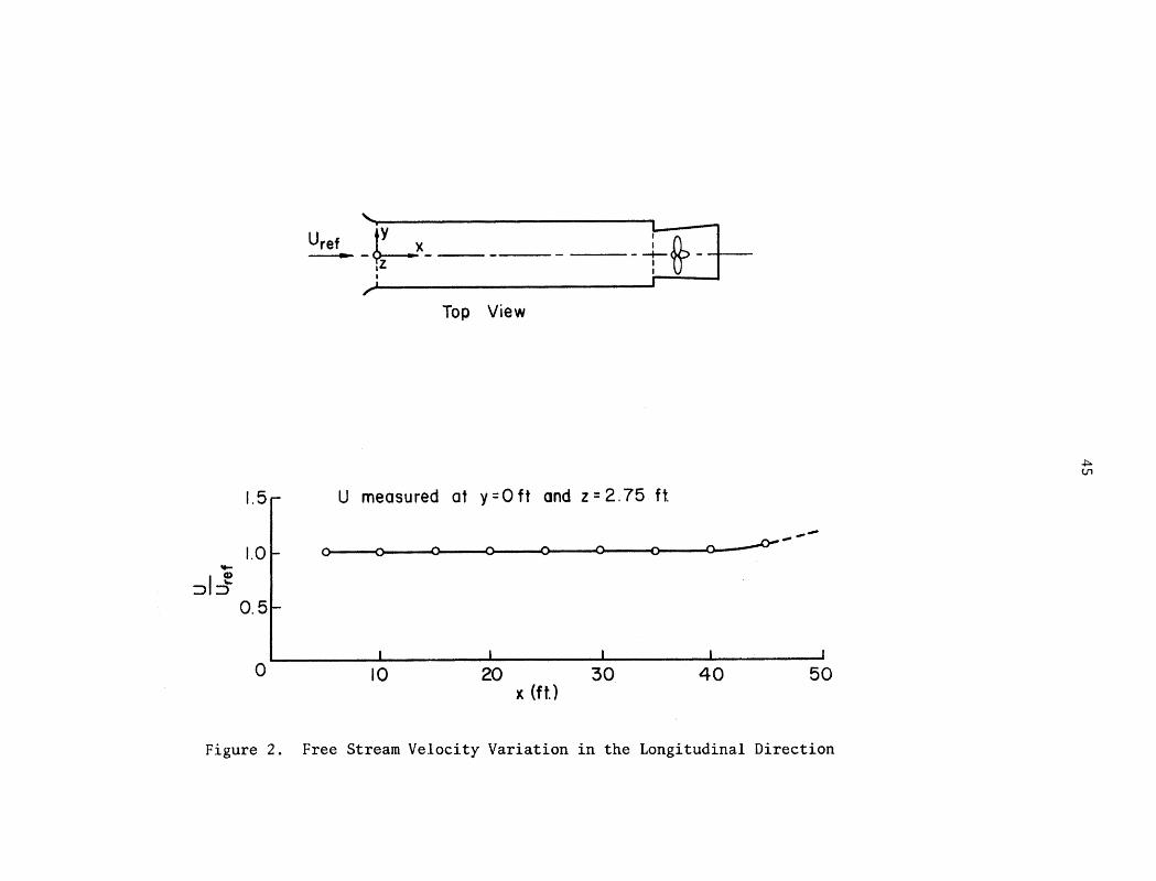
Uref -t:-~- -i~-t-, r

Top View

1.5r U measured at y = 0 ft and z = 2.75 ft

1.01- 0 0 0 0 0 0 0 0 .JJ-"'''*--

o 10 20 30 40 50 x (ft.)

Figure 2. Free Stream Velocity Variation in the Longitudinal Direction

.+;::. V1

46

~ '2.:y-TWO 2"x 2" angles

~e--- -SH-I. 52' .. I

12

10

8 -f/) 0-...... 6 -:::>

4 x = 32' Symbol z (ft.) 0 1.5

2 a 1.0 <> 0.5

q6

12

10

8

-en 0-...... - X = 20' Symbol z (ftJ :::>

0 1.5

2 0 1.0 <> 0.5

0 -6 -5 -4 -3 -2 -I 0 2 3 4 5 6

y (ft. )

Figure 3. Transverse Velocity Distribution at x=20 and 32 ft

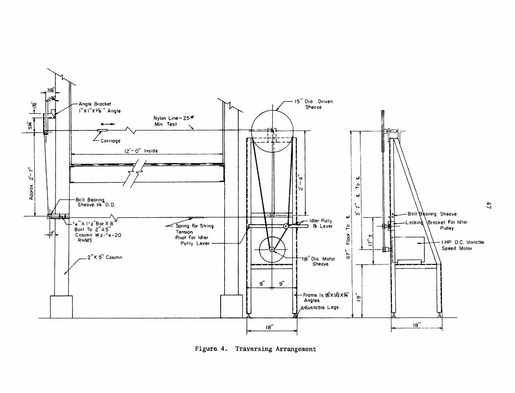
-I'-­

I -N

,( o ~ a. <t

Angle Brocket l"xI"XVa" Angle

---r-, \I ZcOrriOge

'-

~ Nylon Line- 25# Min. Test

" 12'- 0" Inside

I

~ /t J

~ -"~-~1'4"X 112"Bor X 8-:.1 • Bolt To 2"X5"

2. Column W2-'4-20 RHMS

~FOrString Tension II Pivot For Idler

Putty Lever

~

I

I

IS" Dio Driven Sheave

<:;t

I -N

Idler Pully :t:t=::::(;~~::::' a Le ver

-IYl" Dio. Motor Sheove

g" gil

IS"

I.f-Frome Is IrlXIY2XY4' Angles

wAdjUstoble Legs

Figure 4. Traversing Arrangement

.J o I-

= I ~I

~ I

~-

ill

oring Sheave

Bracket For Idler . Pulley

':n IS" 1-------------

::. -...J

WIND TUNNEL TEST SECTION

48

Stainless Steel Miniature Wire Cable

6V D.C. Miniature Electric Valve

~--------------------------121----------------------~~

(Tension

," 12" 0.0. Sheave

Flex i ble ....::::::;.---Ilr--tr ...

Tubing

~85

Tubing

Brass Tubing r'O. Steel Rings I" i 1.0. 12"

Wind Tunnel Floor

Nylon Line- 25 lb. Min. Test

Electric Valve Switch

~ .. Brass Tubing

Flexible Tubing _ To the Wind Tunnel Section

Downwind from the Model

Vacuum Pump Flowmeter

Kr-85 Source Cylinder

Battery

fKr- 85

Figure 5. Schematic Diagram of the Tracer Release System

Glass Jacket

Scaler and

High Voltage

......... ---

<D Valves

-- Tubing

...... --"'" Sample

25 Collector Bottles

• Flow Direction During Sampling

- ..... -- Flow Direction During Transfer

2

Samples from Wind Tunnel

3

+ I I

24

Connector

Figure 6. Sampling System

25

I I I t

By-Pass

Air

I + Reservoir' I I Air

1 Water Il 1 Vacuum

--®­Control Valve

Flow Meter

t Vacuum Pump

Ball Valve

.j:::o. 1.0

o 6000ft I •

~ . '".

'-,,-, /

" ",

/ /

"

Figure 7. Model Lay-Out and Diffusion Sampling Stations

01 ffusion Sampling Statton

Model Field

V1 o

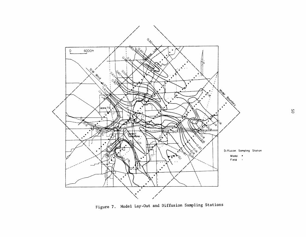
o 6000ft I I

/

y /i

/1

~./ tt-

l' ~,.,

</~, 0' ~o ') ")

_, '/6' u'\... '/6'

////

/ / "

"-"­"-

· .. ·:~",,)t •

% ~

,<90. ,~"

• ,00. . ,~ . "-/

/

)

~I\ ~ ~-~-~IVr=i / ~~n.nl ~~~'hl/

"-"-, /

/ /

Figure 7. Model Lay-Out and Diffusion Sampling Stations

Diffusion Sampling Station

Model • Field

V1 o

1.0

Z Zref O.9

0.8

0.7

0.6

52

1-161-~·1 Model '-'

Fine Roughness

-----.. -- Ure f

Two Rows of 3ft. Long Tubes 2 1/2 in. in Diameter

Velocity Profile Production Arrangement

o Model o Prototype

(Balloon and Tower Data)

Zref = 2500ft.

00 0.1

Figure 9. Comparison of Model and Prototype Velocity Profiles Approaching the City

.L Z'.f

1.0

09

08 o Model

o Prototype Q7

Q6

05

04

03

02

01

0 0 0.1 0.2 0.3 0.35

Turbulence Intensity t Jii u

Figure 10. Comparison of MOdel and Prototype Turbulence Intensities

(J1

<.N

54

20

18

16

>. ~ - TV OM

In 0 Wane Tower u ~ 14

0 G.T. Tower ..... (.) Q)

"0 c: v Mid City 0 ~

N J.4 Q)

--"' 12 > 0

CP -0 II)

0 Q) ..... ~ OM

4-1 0 ... J.4

~ 10 ~

0 >. ~ 'M 0 - 0 .s:; .....

C' Q) 0i) 8 >

I 4-1 0

~ ~ Q)

e Po.

6 0 ..... Q)

> Q) 0

4 ..... ..... Q) J.4 ~ be

OM t1.

2

oL---~--~~~~~~~--L----L ____ L-__ -L __ ~ o 2 3 4 5 6 7 8 9

Wind Velocity, U Ups)

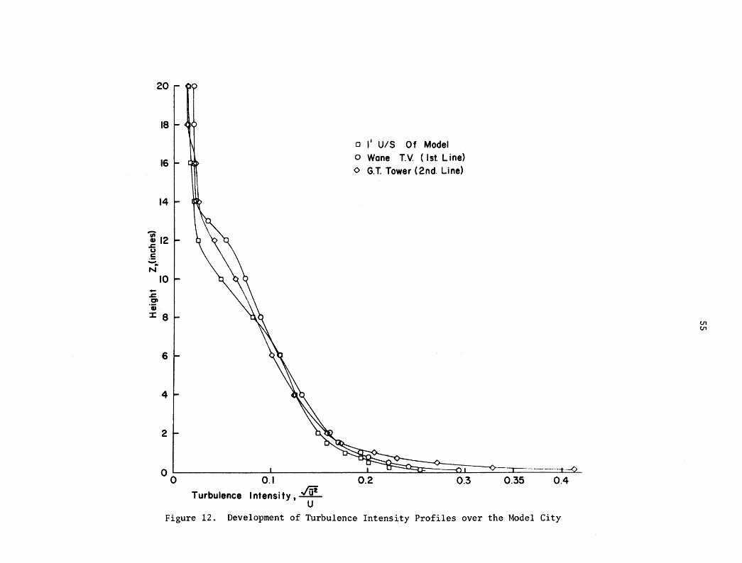
20

18

16

14

:,2 -5 .5 -.. N

10 -.t:: ., 'i J: 8

6

4

2

00 0.1 Jui Turbulence I ntensi ty , _U_

U

o II U/S Of Model

o Wane T.v. (1st Line) <> G.T Tower (2nd. Line)

~----.----.---0.2 0.3 0.35 0.4

Figure 12. Development of Turbulence Intensity Profiles over the Model City

t.n t.n

15 t- v

14

12

10

en 8 • .s::: (,,) c

*' 6 N

-.s::: 01

~ 4

2

o Wane TV. v Mid City

o Station 2 A Station 4

0 1 '~I ~ "A:i: ~ v 50 60 70 80 90 100

Temperature (Of)

Figure 13. Development of Temperature Profiles over the Model City

til a-.

o GOOOh . , I /(

/. t I

~tr-// I

xz~. I /

i'-:>.

y: 0'

'"

/

// /

// "'-" "-

" /' Ii L1

"" ~ .,-1 .. ~ •

.% ~

,<90. ,~.,.

• ,"0'0. . ,~

. '" /

/

)

~~-I/ ~~:~/

"~. /

/ /

Oi ffusion Samphng Station

Model • Field

Figure 14. "Heat Island" Generated Over the Model City

VI "".J

o 6000ft. , I

/

/////

" ", "

"~ ~ ..... ~. ",,[ . . • • ..

•

.~

~ ,<90. ,~'" • ,O'~

• 'Ij.. . '\

~".' _ .. ~, ~t:W~ 1////)

Figure 15 ..

",,- ,/

/ /

"Heat Island" Observed over Fort Wayne

Oi ffusion Sampling Station

Model • Field

V1 00

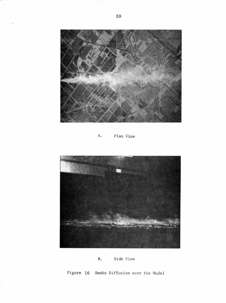
59

A. Plan View

B. Side View

Figure 16 Smoke Diffusion over t he Model

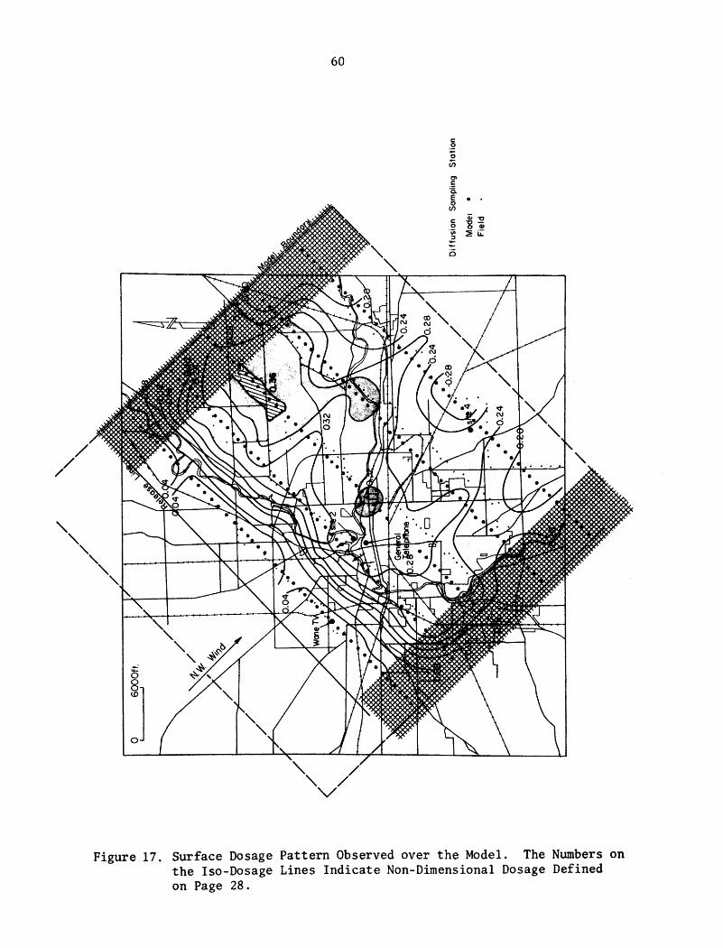
60

Figure 17. Surface Dosage Pattern Observed over the Model. The Numbers on the Iso-Dosage Lines Indicate Non-Dimensional Dosage Defined on Page 28.

~o o·

61

Figure 18. Surface Dosage Pattern Observed In Fort Wayne During Trial 65-06-G2. The Numbers on the Iso-Dosage Lines Indicate Non-Dimensional Dosage Defined on Page 28.

-- . -/ /

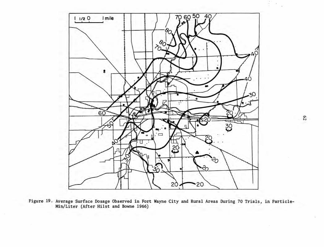
I 1/2 0 I mile

Figure 19. Average Surface Dosage Observed in Fort Wayne City and Rural Areas During 70 Trials, in Particle­Min/Liter (After Hilst and Bowne 1966)

a­N

.4

io II

d .3

CD CJt o

8 CD

~ (/)

_ ,2

§ 'iii

~ :.0 I g Z

.1

I I I I I I r I I

~ 0 f , I \ I , I \ I If \ p.., , y ~ / ~.J

" '0

f 0 tmile ! I

Wind Tunnel Experiments o Runt • Run 2 • 10 Station Average

Field Experiments (TRC) o Trial 6S-06-G2 o 10 Station Average

r'-. 1\ I \ I \ I \ I \

o

I /I 10 ~ "I \ I ( I • .. " ,..i \ I \ I I d '.,./ ~ , f

I I \ \ I /' I f ~ X ~~, I! \ I 1 \ 1\ '\j 'd \.. II \ "~I ~ II \ 1\ ,J \ I I \ 1 \ ~, 0 I \ II \ I \ ' 'lI ,"-1/ ~ I \' \ r-.......) 8 \ I ,1 \ I' I

\ I d '\ }\ I ',yA.i

~ \ I\./ '~ \ I '\. j \ I l>"'"

\1 o - l r Rural Area I· Urban Area ..

Figure 20. Comparison of Model and Field Surface Dosages at 7 Mile Distance from Release Line

(J\ (.N

0.6

.t:::.

:;:).1: 10 0.4 o

II

00

I~' I " , "

With Heat Island } Wind Tunnel

6. ___ Without Heat Island Data

o

o ____ Field Data

Q) c­o U)

I " I " I o

o Q) (J

..E ... :::J (/) 0.2

c c o U) c Q)

E o I c o z

I J I J I , , I I I

o ' «

o 2

" 6-~_b-___ ~ '""-- .

.... ""Z ~_~ __

" " '~

o ----..cL

345 6 7 8 Distance from Source X, (m iles)

-- ----

..............

Figure 21. Longitudinal Variation of Surface Dosages over the Model City and the Prototype

()'\ ~

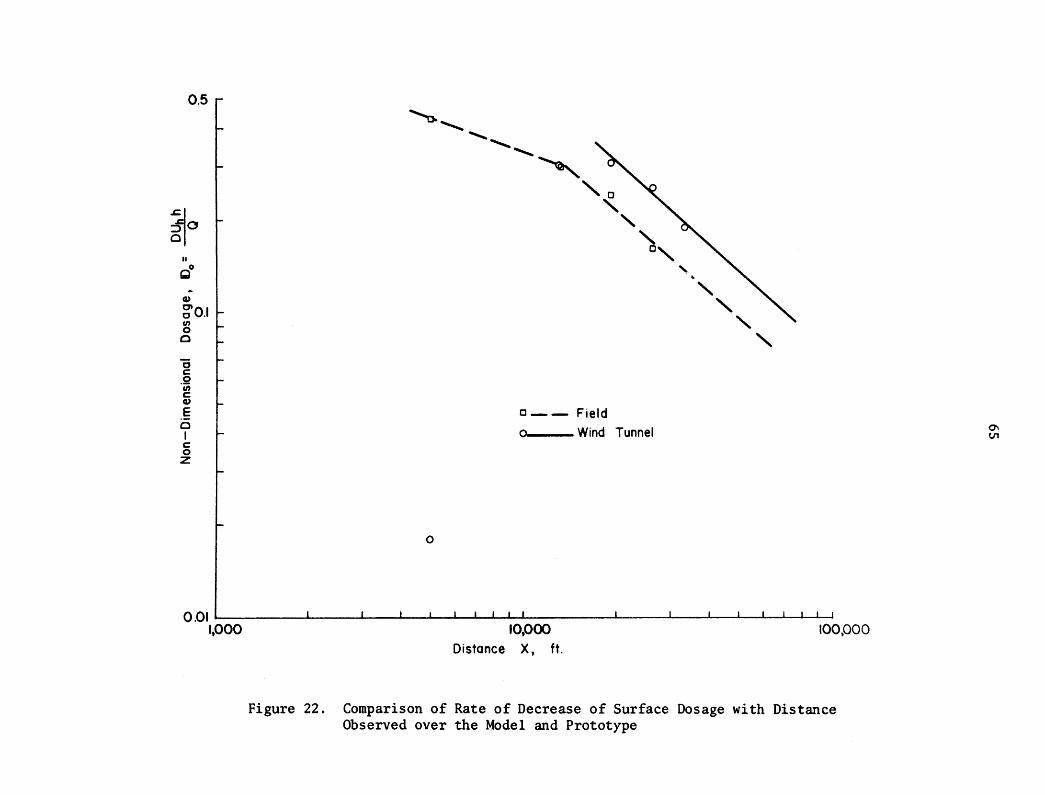
0.5

~o " gO

Q)

gOJ en o o

'0 c .2 en c: CD

E o I c o Z

""-0.." .......................

o

....... , "

"-

0 __ Field

),

o Wind Tunnel

" \0

" " " "

0.01' I I I I ! !

1.000 10.000 100.000 Distance X, ft.

Figure 22. Comparison of Rate of Decrease of Surface Dosage with Distance Observed over the Model and Prototype

0\ V1

1000

-..... b

N

c: 0

..-0 .,. 41

0

-... 0 '0

100 c: 0 <I-CJ)

a (.)

t: • >

10 1,000

r:I

/ /

/ /

/

/ /

66

/

1" /

I I I I I

10.000

Distance X, ft.

/'

,)l/ ,/

/

J/ /

/ /

/ o

/

o Wind Tunnel

- -...0-- Field

Figure 23. Comparison of Field and Wind Tunnel Rates of Vertical Growth of the Cloud

I I

100,000

06

~

.cIa ::> o

II

00

Q) 0.4 C' c (/)

8 Q) o o -... ... ::J en 0°·2 c: o (/) c: Q)

E o I c: o Z

Smith's Model o Wind Tunnel Experiment

o

o

° .-----------------------------------------------------------------------------------~ ° 2

Non- Dimensional Distance from Source Li ne

3 t=~

U2 h h

4

Figure 24. Comparison of Surface Dosages Observed over the Model with those Predicted from Smith's Theory

0\ -......]

fj; CD .c 0 .S

N

-.c 0 'i) :1:

4

3

2

68

--0-

0.2 Non -Dimensional Dosaoe

Smith's Model Wind Tunnel

---

DU h 0.3 [0=--

Q

0.4

Figure 25. Comparison of Vertical Dosage Profile Observed at the First Sampling Line in the Model with Smith's Theory.

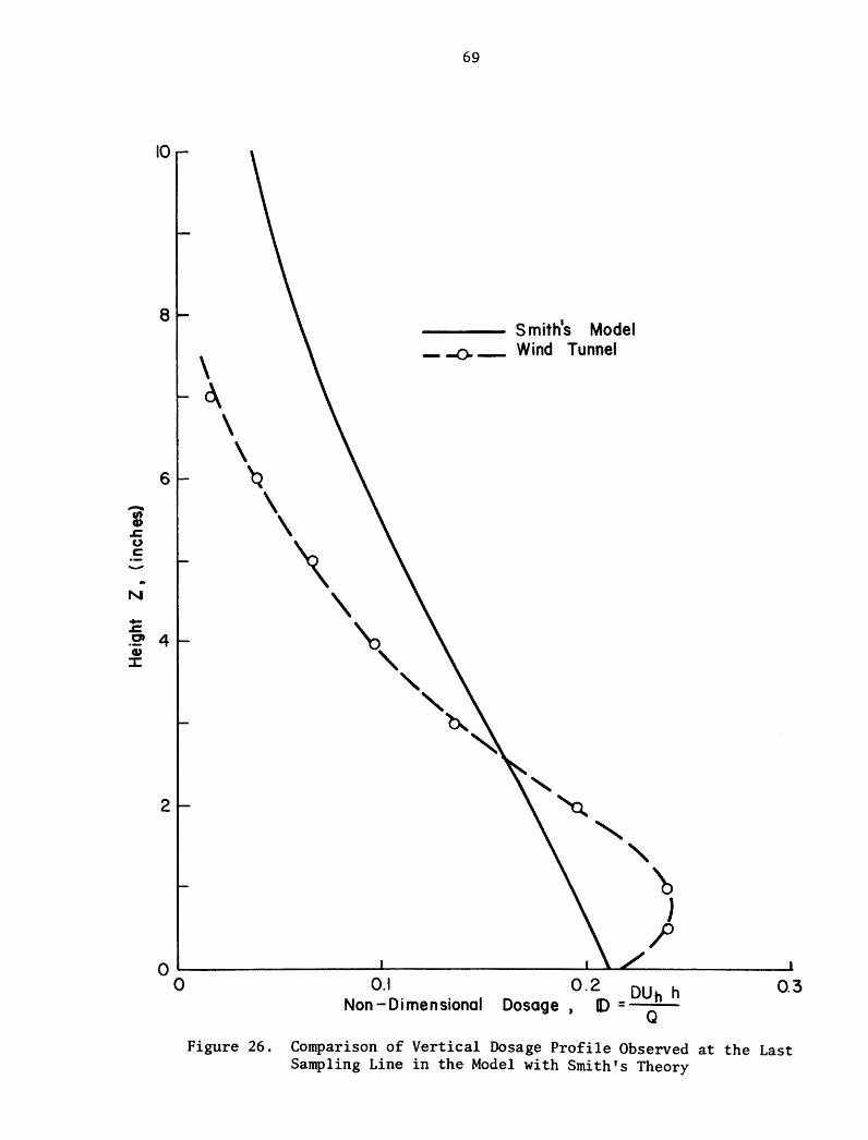
10

8

6

-fh CI)

.c. 0 c: -

N

....

.c.

.2' 4 CI)

::J:

2

0 0

69

Smith's Model

\ _ -0- _ Wind Tunnel

c\ \ \ ~ \ \

\ \

\,

" " " ~ ~ " ~

'" " b J

I' 0.1 0.2 DUh h 0.3

Non -Dimensional Dosage J D= Q

Figure 26. Comparison of Vertical Dosage Profile Observed at the Last Sampling Line in the Model with Smith's Theory

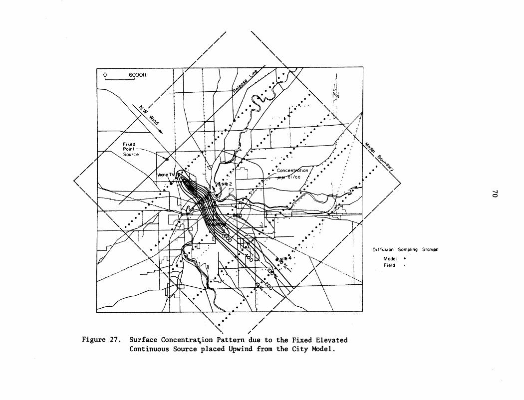
o GooOH. I •

///

// /

", ", !

~ ~ " ~~ " "

,~o ,~.., . ,~ . "\:~ . '\

/ /

)

:t:~ c:(~ 1//

~ Figure 27. Surface Concentra~ion Pattern due to the Fixed Elevated

Continuous Source placed Upwind from the City Model.

Diffusion Sampling StollG)(l

Model • Field

......:I o

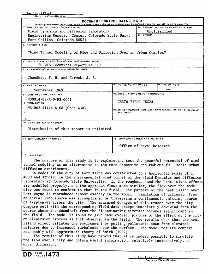
IInel ass; f; ed Securtty Classification

DOCUMENT CONTROL DATA - R&D j§ecuritv classifieation of title boc!.E. of abstract and mdexi'!S.. annotatron must be entered when the overall report is classified)

1. ORIGINATING ACTIVITY (Corporate Bllthor) 28. REPORT SECURITY CLASSIFICATION

Fluid Dynamics and Diffusion Laboratory Engineering Research Center, Colorado State Univ. Fort Collins, Colorado 80521

Unclassified lb. GROUP

3. REPORT TITLE

"Wind Tunnel Modeling of Flow and Diffusion Over an Urban Complex"

4. DESCRIPTIVE NOTES (Type 01 report and Inclusive dates)

THEMIS Technical Report No. 17 5. AUTHORISI (First name, middle initIal, last name)

Chaudhry, F. H. and Cermak, J. E.

6- REPORT DATE

Sep~tember 1969 8d CONTRACT OR GRANT NO.

N00014-68-A-0493-0001 b. PROJ ECT NO.

NR 062-414/6-6-68 (Code 438)

d.

10. DISTRIBUTION ST ATEMENT

Distribution of this report is unlimited

11. SUPPLEMC:NTARY NOTES

13 ABSTRACT

7n. TOT AL NO. OF PAGES

17b. NO. OF REFS

.27 9a. ORIGINATOR'S REPORT NUMBER'S)

CER70-7lFHC-JEC24

9b. OT HER REPORT NOIS) (Any other numbers that ma)· be Bssigned thIs report)

12. SPONSORING MILITARY ACTIVITY

Office of Naval Research

The purpose of this study is to explore and test the powerful potential of wind­tunnel modeling as an alternative to the more expensive and tedious full-scale urban diffusion experiments.

A model of the city of Fort Wayne was constructed to a horizontal scale of 1: 4000 and studied in the environmental wind tunnel of the Fluid Dynamics and Diffusion Laboratory at Colorado State University. If the roughness and the heat-island effects are modelled properly, and the approach flows made similar, the flow over the model city was found to conform to that in the field. The pattern of the heat island over Fort Wayne is reproduced almost exactly in the model. Simulation of diffusion from an aerial line source was accomplished by traversing a continuously emitting source of Krypton-85 across the city. The measured dosages of this tracer over the city compare well with the corresponding field data except immediately downwind from the source where the downdraft from the disseminating aircraft becomes significant in the field. The model is found to give same overall picture of the effect of the city on dispersion process as that observed in the field. The results show that the heat island effect vitiates the environment by pulling pollutants down from elevated releases due to increased turbulence near the surface. The model results compare reasonably with approximate theory of Smith (1957).

The results of this study have proved that it is indeed possible to simulate the flow over a city and obtain useful information, relatively inexpensively, on urban diffusion.

~-------------------------------------------------------------------------------: IIne l ass; fj ed

Security Classification

Unclassified Security Classification

14 LINK A LINK 8 LINK C

KEY WORDS ROLE WT ROLE WT ROLE WT

Atmospheric Simulation

Urban Diffusion Models

Urban Planning

Urban Atmosphere

"Heat Island" effect

Diffusion

Air Pollution Meteorology

Wind Tunnel Modeling

Turbulent Boundary Layer

I

Unclassified Security Classification

April 1971

DISTRIBUTION LIST FOR UNCLASSIFIED TECHNICAL REPORTS ISSUED UNDER

CONTRACT N00014-68-A TASK 000-414 0493-0001

Defense Documentation Center Cameron Station Alexandria, Virginia 22314

Technical Library

(12)

Naval Ship Research and Development Laboratory Annapolis, Maryland 21402

Professor Bruce Johnson Engineering Department Naval Academy Annapolis, Maryland 21402

Library Naval Academy Annapolis, Maryland 21402

Professor W.R. Debler Department of Engineering Mechanics University of Michigan Ann Arbor, Michigan 48108

Professor W.P. Graebel Department of Engineering Mechanics University of Michigan College of Engineering Ann Arbor, Michigan 48108

Professor Finn C. Michelsen Naval Architecture and Marine Engineering 445 West Engineering Building University of Michigan Ann Arbor, Michigan 48108

Dr. Francis Ogilvie Department of Naval Architecture and Marine Engineering University of Michigan Ann Arbor, Michigan 48108

Professor W.W. Willmarth Department of Aerospace Engineering University of Michigan Ann Arbor, Michigan 48108

Dr. S.A. Piacsek Argonne National Laboratory Applied Mathematics Division 9700 S. Cass Avenue Argonne, Illinois 60439

AFOSR (REM) 1400 Wilson Boulevard Arlington, Virginia 22204

Professor S. Corrsin l-fechanics Department The Johns Hopkins University Baltimore, Maryland 20910

Professor L.S.G. Kovasznay The Johns Hopkins University Baltimore, ~1aryland 20910

Professor O.M. Phillips The Johns Hopkins University Baltimore, Maryland 20910

Librarian Department of Naval Architecture University of California Berkeley, California 94720

Professor Israel Cornet Department of Mechanical Engineering University of California Berkeley, California 94720

Professor M. Holt Division of Aeronautical Sciences University of California Berkeley, California 94720

Professor E.V. Laitone Department of Mechanical Engineering University of California Berkeley, California 94720

Professor P. Lieber Department of Mechanical Engineering University of California Institute of Engineering Research Berkeley, California 94720

Professor J.R. Paulling Department of Naval Architecture University of California Berkeley, California 94720

Professor J.V. Wehausen Department of Naval Architecture University of California Berkeley, California 94720

Professor E.R. van Driest Virginia Polytechnic Institute and University Department of Aerospace Engineering Blacksburg, Virginia 24061

Conunander Boston Naval Shipyard Boston, Massachusetts 02129

Director Office of Naval Research Branch Office 495 Sununer Street Boston, Massachusetts 02210

Conunander Puget Sound Naval Shipyard Bremerton, Washington 98314

Professor J.J. Foody Chairman, Engineering Department State University of Ne\~ York Maritime College Bronx, New York 10465

Dr. Alfred Ritter Assistant Head, Applied ~Iechanics Department Cornell Aeronautical Laboratorr, Inc. Buffalo, New York 14221

Dr. J .W. MorTis Manager, Material Sciences Section Advanced Materials Research Bell Aerospace Company P.O. Box 1 Buffalo, New York 14240

Professor G.H. Carrier Department of Engineering and Applied Physics Harvard University Cambridge, Massachusetts 02138

Commanding Officer NROTC Naval Administrative UT_lt Massachusetts Institute of Technology Cambridge, Massachusetts 02139

Professor ~1.A. Abkowitz Department of Naval Architecture and Marine Engineering Massachusetts Institute of Technology Cambridge, Massachusetts 02139

Professor A.T. Ippen Department of Civil Engineering Massachusetts Institute of Technology Cambridge, Massachusetts 02139

Professor L.N. Howard Department of Mathematics Massachusetts Institute of Technology Cambridge, Massachusetts 02139

Professor E.W. Merrill Department of Mathematics Massachusetts Institute of Technology Cambridge, Massachusetts 02139

Professor E. Mollo-Christensen Room 54-1722 Massachusetts Institute of Technology Cambridge, Massachusetts 02139

Professor N. Newman Department of Naval Architecture and Marine Engineering Massachusetts Institute of Technology Cambridge, Massachusetts 02139

Professor A.H. Shapiro Department of Mechanical Engineering Massachusetts Institute of Technology Cambridge, Massachusetts 02139

Commander Charleston Naval Shipyard U.S. Naval Base Charleston, South Carolina 29408

A.R. Kuhlthau, Director Research Laboratories for the Engineering Sciences Thorton Hall, University of Virginia Charlottesville, Virginia 22903

Director Office of Naval Research Branch Office 536 South Clark Street Chicago, Illinois 60605

Library Naval Weapons Center China Lake, California 93555

2

Professor J.M. Burgers Institute of Fluid Dynamics and Applied Hathematics University of Maryland College Park, Maryland 20742

Professor Pai Institute for Fluid Dynamics and Applied r.tathematics University of Maryland College Park, Maryland 20740

Acquisition Director NASA Scientific & Technical Information P.O. Box 33 College Park, Maryland 20740

Technical Library Naval Weapons Laboratory Dahlgren, Virginia 22448

Computation & Analyses Laboratory Naval Weapons Laboratory Dahlgren, Virginia 22448

Dr. C.S. Wells, Jr. Manager - Fluid Mechanics Advanced Technology Center, Inc. P.O. Box 6144 Dallas, Texas 75222

Dr. R.H. Kraichnan Dublin, New Hampshire 03444

Commanding Officer Army Research Office Box CM, Duke Station Durham, North Carolina 27706

Professor A. Charnes The Technological Institute Northwestern University Evanston, Illinois 60201

Dr. Martin H. Bloom Polytechnic Institute of Brooklyn Graduate Center, Dept. of Aerospace Engineering and Applied Mechanics Farmingdale, New York 11735

Technical Documents Center Building 315 U.S. Army Mobility Equipment Research and Development Center Fort Belvoir, Virginia 22060

Professor J.E. Cermak College of Engineering Colorado State University Ft. Collins, Colorado 80521

Technical Library Webb Institute of Naval Architecture Glen Cove, Long Island, New York 11542

Professor E.V. Lewis Webb Institute of Naval Architecture Glen Cove, Long Island, New York 11542

Dr. B.N. Pridmore Brown Northrop Corporation NORAIR-Div. Hawthorne, Caiifornia 90250

Dr. J. P. Bres lin Stevens Institute of Technology Davidson Laboratory Hoboken, New Jersey 07030

Dr. D. Savitsky Stevens Institute of Technology Davidson Laboratory Hoboken, New Jersey 07030

Mr. C.H. Henry Stevens Institute of Technology Davidson Laboratory Hoboken, New Jersey 07030

Dr. J.P. Craven University of Hawaii 1801 University Avenue Honolulu, Hawaii 96822

Professor E.L. Resler Graduate School of Aeronautical Engineering Cornell University Ithaca, New York 14851

Professor John Miles c/o I.G.P.P. University of California, San Diego La Jolla, California 92038

Director Scrippe Institution of Oceanography University of California La Jolla, California 92037

Professor A. Ellis University of California, San Diego Department of Aerospace & Mechanical Engineering La Jolla, California 92037

Dr. B. Sternlicht Mechanical Technology Incorporated 968 Albany-Shaker Road Latham, New York 12110

Dr. Coda Pan Mechanical Technology Incorporated 968 Albany-Shaker Road Latham, New York 12110

Mr. P. Eisenberg, President Hydronautics, Inc. Pindell School Road Howard County Laurel, Maryland 20810

Mr. M.P. Tulin Hydronautics, Inc. Pindell School Road Howard County Laurel, Maryland 20810

Mr. Alfonso Alcedan L.,Director Laboratorio Nacional De Hydraulics Antigui Cameno A. Ancon Casilla Jostal 682 Lima, Peru

Commander Long Beach Naval Shipyard Long Beach, California 90802

3

Professor John Laufer Department of Aerospace Engineering University Park Los Angeles, California 90007

Professor .J .~1. Killen St. Anthony Falls Hydraulic Lab. University of Minnesota Minneapolis, ~1innesota 55414

Lorenz G. Straub Library St. Anthony Falls Hydraulic Lab. Mississippi River at 3rd Avenue S.E. Minneapolis, Minnesota 55414

Professor J. Ripkin St. Anthony Falls Hydraulic Lab. University of Minnesota Minneapolis, Minnesota 55414

Dr. W. Silberman St. Anthony Falls Hydraulic Lab. Mississippi River at 3rd Avenue S.E. ~1inneapolis, Minnesota 55414

Superintendent Naval Postgraduate School Library Code 0212 Monterey, California 93940

Professor A.B. Metzner University of Delaware Newark, New Jersey 19711

Technical Library Naval Underwater Systems Center Newport, Rhode Island 02840

Professor Dudley D. Fuller Department of Mechanical Engineering Columbia University New York, New York 10027

Professor V. Castelli Department of Mechanical Engineering Columbia University New York, New York 10027

Professor H. Elrod Department of Mechanical Engineering Columbia University New York, New York 10027

Professor J.J. Stoker Institute of Mathematical Sciences New York University 251 Mercer Street New York, New York 10003

Society of Naval Architects and t-tarine Engineering 74 Trinity Place New York, New York 10006

Engineering Societies Library 345 East 47th Street New York, New York 10017

Office of Naval Research New York Area Office 207 W. 24th Street New York. New York 10011

~fiss O.M. Leach, Librarian National Research Council Aeronautical Library Montreal Road Ottawa 7, Canada

Technical Library Naval Ship Research and Development Center Panama City, Florida 32401

Technical Library Naval Undersea R&D Center Pasadena Laboratory 3202 E. Foothill Boulevard Pasadena, California 91107

Dr. Andrew Fabula Naval Undersea Research & Development Center Pasadena Laboratory 3202 E. Foothill Boulevard Pasadena, California 91107

Dr. J.W. Hoyt Naval Undersea R&D Center Pasadena Laboratory 3202 E. Foothill Boulevard Pasadena, California 91107

Professor A. Acosta Department of Mechanical Engineering California Institute of Technology Pasadena, California 91109

Professor H. Liepmann Department of Aeronautics California Institute of Technology Pasadena, California 91109

Professor M.S. Plesset Engineering Division California Institute of Technology Pasadena, California 91109

Professor A. Roshko California Institute of Technology Pasadena, California 91109

Professor T.Y. Wu Department of Engineering California Institute of Technology Pasadena, California 91109

Director Office of Naval Research Branch Office 1030 E. Green Street Pasadena, California 91101

Naval Ship Engineering Center Philadelphia Division Technical Library Philadelphia, Pennsylvania 19112

Technical Library Philadelphia Naval Shipyard Philadelphia, Pennsylvania 19112

Professor R.C. Mac Camy Department of t-tathematics Carnegie Institute of Technology Pittsburgh, Pennsylvania 15213

4

Dr. Paul Kaplan Oceanics, Inc. Plainview, Long Island, New York 11803

Technical Library Naval Missile Center Point ~fugu, California 93441

Technical Library Naval Civil Engineering Laboratory Port Hueneme, California 93041

Commander Portsmouth Naval Shipyard Portsmouth, New Hampshire 03801

Commander Norfolk Naval Shipyard Portsmouth, Virginia 23709

Professor F.E. Bisshopp Division of Engineering Brown University Providence, Rhode Island 02912

Dr. William A. Gross, Vice President Ampex Corporation 401 Broadway Redwood City, California 94063

Dr. H.N. Abramson Southwest Research Institute 8500 Culebra Road San Antonio, Texas 78228

Editor Applied Mechanics Review Southwest Research Institute 8500 Culebra Road San Antonio, Texas 78206

Office of Naval Research San Francisco Area Office 50 Fell Street San Francisco, California 94102

Library Pearl Harbor Naval Shipyard Box 400 FPO San Francisco, California 96610

Technical Library Hunters Point Naval Shipyard San Francisco, California 94135

Librarian Naval Ordnance Laboratory White Oak Silver Spring, r.1aryland 20910

Fenton Kennedy Document Library The Johns Hopkins University Applied Physics Laboratory 8621 Georgia Avenue Silver Spring, Maryland 20910

Professor E.Y. Hsu Department of Civil Engineering Stanford University Stanford, California 94305

Dr. Byrne Perry Department of Civil Engineering Stanford University Stanford, California 94305

Dr. R. L. Street Department of Civil Engineering Stanford University Stanford, California 94305

Professor Milton Van Dyke Department of Aeronautical Engineering Stanford University Stanford, California 94305

Professor R.C. Di Prima Department of Mathematics Rensselaer Polytechnic Institute Troy, New York 12180

Professor J. Lumley Ordnance Research Laboratory Pennsylvania State University University Park, Pennsylvania 16801

Dr. M. Sevik Ordnance Research Laboratory Pennsylvania State University University Park, Pennsylvania 16801

Dr. J.M. Robertson Department of Theoretical and Applied Mechanics University of Illinois Urbana, Illinois 61803

Technical Library Mare Island Naval Shipyard Vallejo, California 94592

Code 438 Office of Naval Research Department of the Navy Arlington, Virginia 22217

Code 461 Office of Naval Research Department of the Navy Arlington, Virginia 22217

Code 463 Office of Naval Research Department of the Navy Arlington, Virginia 22217

Code 472 Office of Naval Research Department of the Navy Arlington, Virginia 22217

Code 468 Office of Naval Research Department of the Navy Arlington, Virginia 22217

Code 473 Office of Naval Research Department of the Navy Arlington, Virginia 22217

Code 481 Office of Naval Research Department of the Navy Arlington, Virginia 22217

(3)

5

Code 2627 Naval Research Laboratory Washington, D.C. 20390

Library, Code 2620 (ONRL) Naval Research Laboratory Washington, D.C. 20390

Code 6170 Naval Research Laboratory Washington, D.C. 20390

Code 4000 Director of Research Naval Research Laboratory Washington, D.C. 20390

Code 8030 (Maury Center) Naval Research Laboratory Washington, D.C. 20390

Code 8040 Naval Research Laboratory Washington, D.C. 20390

Code 031 Naval Ship Systems Command Washington, D.C. 20390

Code 0341 Naval Ship Systems Command Washington, D.C. 20390

Code 034l2B (L. Benen) Naval Ship Systems Command Washington, D.C. 20390

Code 03412 (J. Schuler) Naval Ship Systems Command Washington, D.C. 20390

Code 2052 Naval Ship Systems Command Washington, D. C. 20390

Code 6034 Naval Ship Engineering Center Center Building Prince George's Center Hyattsville, Maryland 20782

Code 6110 Naval Ship Engineering Center Center Building Prince George's Center Hyattsville, Maryland 20782

Code 6113 Naval Ship Engineering Center Center Building Prince George's Center Hyattsvi lIe, ~lary land 20782

Code 6114 Naval Ship Engineering Center Center Building Prince George's Center Hyattsville, ~lary1and 20782

Code 6120E Naval Ship Engineering CeDter Center Building Prince George's Center Hyatts\,i lle, ~Iaryl and :0-:-8:

(6)

(6)

Code 6136 Naval Ship Engineering Center Center Building Prince George's Center Hyattsville, ~1ary1and 20782

Dr. A. Powell Code 01 Naval Ship Research and Development Center Washington, D.C. 20034

Mr. W.M. Ellsworth Code OH50 Naval Ship Research and Development Center Washington, D.C. 20034

Central Library Code L42 Naval Ship Research and Development Center Washington, D.C. 20034

Dr. W.E. Cununins Code 500 Naval Ship Research and Development Center Washington, D.C. 20034

Mr. S.F. Crump Code 513 Naval Ship Research and Development Center Washington, D.C. 20034

Mr. R. Wermter Code 520 Naval Ship Research and Development Center Washington, D.C. 20034

Dr. P. Pien Code 521 Naval Ship Research and Development Center Washington, D.C. 20034

Dr. W.B. Morgan Code 540 Naval Ship Research and Development Center Washington, D.C. 20034

Mr. P. Granvi lIe Code 541 Naval Ship Research and Development Center Washington, D.C. 20034

Mr. J.B. Hadler Code 560 Naval Ship Research and Development Center Washington, D.C. 20034

Dr. H.R. Chaplin Code 600 Naval Ship Research and Development Center Washington, D.C. 20034

Mr. G.H. G1eissner Code 800 Naval Ship Research and Development Center Washington, D.C. 20034

Dr. M. Strasberg Code 901 Naval Ship Research and Development Center Washington, D.C. 20034

6

Mr. J. HcCarthy Code 552 Naval Ship Research and Development Center Washington, D.C. 20034

Code 03 Naval Air Systems Command Washington, D.C. 20360

AIR 5301 Naval Air Systems Command Department of the Navy Washington, D.C. 20360

Code ORD 03 Naval Ordnance Systems Conunand Washington, D.C. 20360

Code ORO 035 Naval Ordnance Systems Conunand Washington, D.C. 20360

Code ORD 05413 Naval Ordnance Systems Conunand Washington, D.C. 20360

Code ORO 9132 Naval Ordnance Systems Conunand Washington, D.C. 20360

Oceanographer of the Navy Washington, D.C. 20390

Conunander Naval Oceanographic Office Washington, D.C. 20390

Chief Scientist (CNM PM-I) Strategic Systems Project Office Department of the Navy Washington, D.C. 20360

Technical Division (CNM PM 11-20) Deep Submergence Systems Project Office Department of the Navy Washington, D.C. 20360

Dr. A.L. Slafkosky Scientific Advisor Conunandant of the Marine Corps (Code AX) Washington, D.C. 20380

Librarian Station 5-2 Coast Guard Headquarters NASSIF Building 400 7th Street, S.W. Washington, D.C. 20591

Office of Research and Development Maritime Administration 441 G. Street, N.W. Washington, D.C. 20235

Division of Ship Design Maritime Administration 441 G. Street, N.W. Washington, D.C. ~0235

National Science Foundation Engineering Division 1800 G. Street, N.W. Washington, D.C. 20550

Dr. G. Ku1in National Bureau of Standards Washington, D.C. 20234

Science & Technology Division Library of Congress Washington, D.C. 20540

Chief of Research & Development Office of Chief of Staff Department of the Army The Pentagon, Washington, D.C. 20310

Professor A. Thiruvengadam Department of Mechanical Engineering The Catholic University of America Washington, D.C. 20017

Professor G. BiTkhoff Department of Mathematics Harvard University Cambridge, Massachusetts 02138

AIR 604 Naval Air Systems Command Department of the Navy Washington, D.C. 20360

7

Dr. A.S. Iberall, President General Technical Services, Inc. 451 Penn Street Yeadon, Pennsylvania 19050

Professor J.F. Kennedy, Director Iowa Institute of Hydraulic Research State University of Iowa Iowa City, Iowa 52240

Professor L. Landweber Iowa Institute of Hydraulic Research State University of Iowa Iowa City, Iowa 52240

Dr. Lee Segel Department of Mathematics Rensselaer Polytechnic Institute Troy, New York 12180

Code 6101E Naval Ship Engineering Center Center Building Prince George's Center Hyattsville, Maryland 20782