project report

1

CHAPTER 1

INTRODUCTION

1.1 GENERAL

The Thannermukkom salt water barrier was constructed as a part of the Kuttanad Development

Scheme to prevent tidal action and intrusion of salt water into the Kuttanad low-lands across

Vembanad Lake between Thannermukkom on South and Vechur on North. It is the largest mud

regulator in India. This barrier essentially divides the lake into two parts - one with brackish

water perennially and the other half with fresh water fed by the rivers draining in to the lake. The

TMB was planned to be of 1402m length with 93 shutters. The TMB was commissioned to

prevent saline intrusion from Cochin gut into the southern part of Vembanad Lake (where paddy

cultivation is practised) to protect the crop from damage from saltwater intrusion. The plan was

to build the Thannermukkom Barrage in three phases. The first phase at Thannermukkom end

comprising 31 shutters and 2 locks for navigation was completed in 1968. The second phase at

Vechoor end with 31 shutters and one lock was completed in 1974. When the work on the third

phase with 31 shutters was delayed, a coffer dam was erected in 1975 to stop the salt water flow.

The expected benefit from TBM was safe punja paddy and the intensification to a second

crop(virippu crop) in about 18,500 ha of kayal and lower kuttanad.

Though the partial commissioning of the barrage could prevent the saline water to the southern

side and thereby supported paddy cultivation, it created several problems in the wet land system,

the major ones are

(1) Concentration of pollutants due to inadequate tidal flushing due to closure of the bund and

due to blockage at the centre 1/3rd portion(ie coffer dam)

(2) Reduction in flood discharge during monsoon as the central 1/3rd portion is blocked

(3) Silting at the southern side of the barrage

During 2007, Union Ministry of Agriculture invited M.S.SWAMINATHAN RESEARCH

FOUNDATION (MSSRSF) for a detailed study of the economic and ecological problems of the

Alappuzha district as well as the Kuttanad wetland ecosystem as a whole and to recommend the

possible solutions. One of the recommendations given by MSSRF is as follows.

2

1.2 MEASURES FOR SALINITY AND FLOOD MANAGEMENT IN KUTTANAD

1. Undertake and complete the work on phase 3 of the TMB following modern design,

compatible with the renovated phase 1 and phase 2 portions and with all shutters operatable.

2. Dismantle and remove the coffer dam without letting the soil and debris spreading on the lake

bed. Dredge the part of Lake south of the coffer dam to suitable depth based on proper

bathymetric studies and gradient analysis.

We feel that the construction of third stage of Thenneermukkom barrage is the need of the hour

and hence we choose the design of third stage as project.

Fig 1.1 : Thanneermukkom Salt Water Barrier

3

CHAPTER 2

LITERATURE REVIEW

2.1 GENERAL

The main purpose of Thanneermukkom salt water barrier is to protect paddy cultivation on

Kuttanad area from saline intrusion from Cochin gut. At the same time, water transport and land

transport across the site should not be affected. To maintain water transport, lock gates are

constructed and to maintain land transport, the bridge is constructed. Since our project is limited

to central portion which is presently a coffer dam and is being replaced by a concrete bridge

structure with regulators, only the design of central portion is included. After comparison of

different types of section of girders, T beam girder is selected. The shape and height of pier

selected has also their own significance. Different papers from which information gathered for

the progress of the project work are included in this section.

2.2 ARTICLE DETAILS

Arnold W. Hendry , Leslie G. Jaeger(1955) in their article ―The Load Distribution in

Interconnected Bridge Girders with Special Reference to Continuous Beams” explained about

how a method which is usually applied to a simply supported beam, can be applied to analysis of

an interconnected continuous beam. The method outlined is for the analysis of interconnected

bridge girders having any degree of torsional rigidity and is based on two assumptions that the

transverse members can be replaced by a continuous medium and that torsion of these members

can be neglected. The solution is reached by harmonic analysis and distribution coefficients are

tabulated for single span bridges having from two to six main girders for all harmonics of the

bending moment and deflection curves for the span. The application of the method to continuous

beam systems by superposition is also explained. A method for the derivation of influence lines

for bending moments in the longitudinals of continuous bridges is also developed.

Mundzir Hasan Basri (2001), in the article “Two New Methods for Optimal Design of

Subsurface Barrier to Control Seawater Intrusion” analysed two new methods to control

seawater intrusion using a subsurface barrier through development and application of the implicit

and explicit simulation-optimization approaches and had developed implicit and explicit

4

simulation-optimization models for design of a subsurface barrier that controls seawater

intrusion. No prior work has been done in which a model for optimal design of a barrier for

controlling seawater intrusion is developed. The objective of the seawater intrusion control

problem is to minimize the total construction costs while requiring that salt concentrations be

held below specified values at two control locations at the end of the design period.

Nan Hu and Gonglian Dai (2010) in the article “The Comparative Study of Portal-Frame Pier

for High-Speed Railway” explained about the performance of portal-frame pier. They proved

that it not only provides comfort of passengers but also the safety of the vehicles. The study was

made by the comparison of five different portal-frame piers and based on it, the type, selection

for structure design and the effect of different structure parameters on structure performance as

well as stability of vehicle has been analysed.

The essentiality of replacement of central bunded portion of Thanneermukkom salt water barrage

is explained in the report named “Study for modernizing the Thanneermukkom bund and

Thottappally spillway for efficient water management in Kuttanad region, Kerala” (2011)

submitted to Kerala Governmnent on August 2011, based on studies conducted by Indian

Institute of Technology, Madras, Chennai and Centre for Water resources development and

management, Kozhikode, Kerala. The study revealed that the middle bunded portion of the

barrage does not have significant effect on flooding in the study area. But due to the absence of

natural flushing action, accumulation of pollutants occurs in the lake. Improper working of

several existing gates of the barrage also creates problems. The report suggest to replace mud

regulator with a gated structure with provisions for natural flushing and at the same time

restricting the salinity to levels below critical value for normally grown paddy by proper

monitoring of salt concentration.

M.G. Kalyanshetti, C.V. Alkunte (2012) carried out a study for effectiveness of IRC live load for

various height of pier and span of bridge for different shape of pier in the article “Study on

Effectiveness of IRC Live load on R.C.R Bridge Pier”. The effectiveness of IRC live load for

various height of pier and span of bridge for different shape of pier is studied using computer

5

programming. The study reveals that pier designed by considering IRC class A loading should be

checked for IRC 70R wheeled loading.

Parvin Eghbali, Amir Ahmad Dehghani, Hadi Arvanaghi, Maryam Menazadeh (2013) explained

about scouring around bridge foundations which is one of the major causes of bridge damaging

in the article “The Effect of Geometric Parameters and Foundation Depth on Scour Pattern

around Bridge Pier”. The effect of shape, level and position angle of foundation on scour pattern

were investigated experimentally and the results showed that the scour depth depends on

foundation depth, shape and foundation alignment to the approach flow. The best foundation

shape which leads to minimum scour was aerodynamic shape along the channel, square,

aerodynamic across the channel and cylindrical shape respectively, the best positioning of

foundation is that below the initial channel bed and the best angle for positioning of foundation is

zero (parallel to flow direction).

Amit Saxena and Dr.Savita Maru (2013) in the article “Comparative Study of the Analysis and

Design of T-Beam Girder and Box Girder Superstructure” compared T-beam girder and Box

girder to check which among the two is favourable. The decisions were taken based on obvious

element of Engineering - safety, serviceability and economy. They had concluded that service

load bending moments and shear force for T-beam girder are lesser than box girder which allow

the designer to have lesser heavier section for T-beam girder than Box girder for span upto 25m.

Also the cost of concrete and quantity of steel required by the T-beam girder is less.

Manjeetkumar M Nagarmunnoli and S V Itti (2014) in their article “Effect of Deck Thickness in

RCC T-beam Bridge” explained that the increased traffic demand, material ageing, cracking of

bridge components, physical damages incurred by concrete, corrosion of reinforcement and

inadequate maintenance of bridges necessitate the assessment of bridges periodically for their

performances. The non linear analysis is a tool to simulate the exact material behaviour, to

evaluate strength in inelastic range. An attempt has been made to perform non linear finite

element analysis to analyse the component of a selected road bridge. They studied about the

fatigue life evaluation of reinforced Concrete Highway Bridge and has carried out Non-linear

6

analysis of the structural element using ANSYS. RCC T-beam Bridge has been chosen for

detailed 3D nonlinear analysis.

H P Santhosh, Dr. H M Rajashekhara Swamy, Dr. D L Prabhakara (2014) in their article

“Construction Of Cofferdam -A Case Study” explained about the present state of construction of

cofferdam techniques and techniques developed world wide for mitigating hydraulic forces on

the temporary structures. A cofferdam is a temporary structure designed to keep water and soil

out of the excavation in which a bridge pier or other structure is built. When construction must

take place below the water level, a cofferdam is built to give workers a dry work environment.

Sheet piling is driven around the work site, seal concrete is placed into the bottom to prevent

water from seeping in from underneath the sheet piling, and the water is pumped out.

Kavitha.N, Jaya kumari.R, Jeeva.K, Bavithra.K, Kokila.K (2015) in their article “Analysis and

Design of Flyover” conducted a traffic survey at the four road junction in Salem town and

designed all the structural parts for the grade separator. The grade separator is of 640 m length

with 21 spans, 20m per span. It consists of a deck slab, longitudinal girders, cross girders, deck

beam, pier and foundation. Slab is designed by Working stress method as per the

recommendation of IRC:21-2000, Clause 304.2.1. Cantilever slab is designed for maximum

moment due to cantilever action. Longitudinal girders are designed by Courbon‘s method. Cross

girders are designed mainly for stiffness to longitudinal girders. Elastomeric reinforced bearing

plate is used. The deck beam is designed as a cantilever on a pier. The Pier is designed for the

axial dead load and live load from the slab, girders, deck beam. Foundation designed as footing

for the safe load bearing in the soil.

Praful N K and Balaso Hanumant (2015) in their article “Comparative Analysis of T-Beam

Bridge by Rational Method and Staad Pro” explained that the bridge is a structure providing

passage over an obstacle without closing the way beneath. The required passage may be for a

road, a railway, pedestrians, a canal or a pipeline. T-beam bridge decks are one of the principal

types of cast-in place concrete decks. T-beam bridge decks consist of a concrete slab integral

with girders. The finite element method is a general method of structural analysis in which the

solution of a problem in continuum mechanics is approximated by the analysis of an assemblage

7

of finite elements which are interconnected at a finite number of nodal points and represent the

solution domain of the problem. A simple span T-beam bridge was analyzed by using I.R.C.

loadings as a one dimensional structure using rational methods. The same T-beam bridge is

analysed as a three dimensional structure using finite element plate for the deck slab and beam

elements for the main beam using software STAAD ProV8i. Both FEM and 1D models where

subjected to I.R.C. Loadings to produce maximum bending moment, Shear force and similarly

deflection in structure was analysed. The results obtained from the finite element model are

lesser than the results obtained from one dimensional analysis, which means that the results

obtained from manual calculations subjected to IRC loadings are conservative.

8

CHAPTER 3

DESIGN

3.1 GENERAL

A T beam bridge with suitable foundation is designed based on codal provisions. Codes used for

the design are IS 456:2000, SP 16:1980, IRC 6:2000, IRC 21: , IS 2911-1979 (Part 1) and IS

6966 (Part 1): 1989. Following components are designed in this section:

1. Deck slab

2. Cantilever slab

3. Longitudinal girder

4. Cross girder

5. Bearings

6. Pedestals

7. Operating platform

8. Pier

9. Pier cap

10. Pile

11. Pile cap

12. Apron and cut off

Design of pier is done using STAAD.Pro and the remaining components are designed manually.

Designing is done based on data obtained from previous records of similar bridges, study reports

and drawings given from the site and codal provisions.

Given Details

Clear roadway = 7.5m

Effective span of T-beam = 13.22m

Four longitudinal T-beams of thickness 625mm spaced at 2.625m intervals

Five cross beams of thickness 300mm spaced at 3.305m intervals

The preliminary dimensions may be assumed as shown in Fig 5.1. These may be checked later

and modified, if necessary. M30 grade concrete and high yield deformed bars of Fe415 grade

conforming to IS 1786 will be used. Clear cover to reinforcement is taken as 40mm.

9

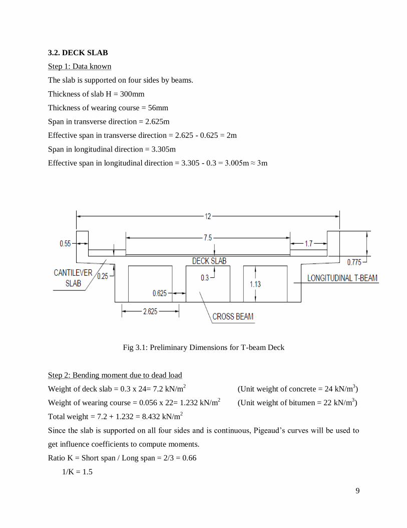
3.2. DECK SLAB

Step 1: Data known

The slab is supported on four sides by beams.

Thickness of slab H = 300mm

Thickness of wearing course = 56mm

Span in transverse direction = 2.625m

Effective span in transverse direction = 2.625 - 0.625 = 2m

Span in longitudinal direction = 3.305m

Effective span in longitudinal direction = 3.305 - 0.3 = 3.005m ≈ 3m

Fig 3.1: Preliminary Dimensions for T-beam Deck

Step 2: Bending moment due to dead load

Weight of deck slab = 0.3 x 24= 7.2 kN/m2

(Unit weight of concrete = 24 kN/m3)

Weight of wearing course = 0.056 x 22= 1.232 kN/m2

(Unit weight of bitumen = 22 kN/m3)

Total weight = 7.2 + 1.232 = 8.432 kN/m2

Since the slab is supported on all four sides and is continuous, Pigeaud‘s curves will be used to

get influence coefficients to compute moments.

Ratio K = Short span / Long span = 2/3 = 0.66

1/K = 1.5

10

From Pigeaud‘s curves, m1 = 0.045 and m2 = 0.018

Total dead weight W = 8.432 x 2 x 3 = 50.6 kN

Moment along short span = W (m1 + 0.15m2) = 50.6 [0.045 + (0.15 x 0.018)] = 2.42kNm

Moment along long span = W (m2 + 0.15m1) = 50.6 [0.018 + (0.15 x 0.045)] = 1.25kNm

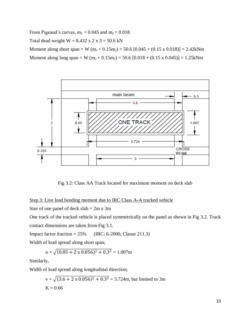
Fig 3.2: Class AA Track located for maximum moment on deck slab

Step 3: Live load bending moment due to IRC Class A-A tracked vehicle

Size of one panel of deck slab = 2m x 3m

One track of the tracked vehicle is placed symmetrically on the panel as shown in Fig 3.2. Track

contact dimensions are taken from Fig 3.1.

Impact factor fraction = 25% (IRC: 6-2000, Clause 211.3)

Width of load spread along short span;

u = 0.85 + 2 x 0.056 2 + 0.32 = 1.007m

Similarly,

Width of load spread along longitudinal direction;

v = 3.6 + 2 x 0.056 2 + 0.32 = 3.724m, but limited to 3m

K = 0.66

11

u/B = 1.007/2 = 0.503

v/L = 3/3 = 1

Using Pigeaud‘s curve for K= 0.7,

m1 = 7.6x 10-2

m2 = 3.1 x 10-2

Total load per track including impact = 1.25 x 350 (Fig 1, , IRC:6-2000)

= 437.5kN

Effective load on the span W = 437.5 x (3/ 3.724) = 352.44 kN

Moment along shorter span = W (m1 + 0.15m2) = 352.44 [(7.6 + 0.15x3.1) x 10-2

] = 28.42kNm

Moment along longer span = W (m2 + 0.15m1) = 352.44 [(3.1 + 0.15x7.6) x 10-2

] = 14.94kNm

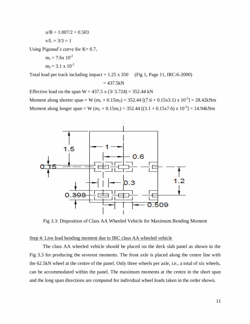
Fig 3.3: Disposition of Class AA Wheeled Vehicle for Maximum Bending Moment

Step 4: Live load bending moment due to IRC class AA wheeled vehicle

The class AA wheeled vehicle should be placed on the deck slab panel as shown in the

Fig 3.3 for producing the severest moments. The front axle is placed along the centre line with

the 62.5kN wheel at the centre of the panel. Only three wheels per axle, i.e., a total of six wheels,

can be accommodated within the panel. The maximum moments at the centre in the short span

and the long span directions are computed for individual wheel loads taken in the order shown.

12

(a) B.M due to wheel 1

Consider the load marked 1 in fig.

Tyre contact dimensions are 300 x 150 mm

u = 0.3 + 2x0.056 2 + 0.32 = 0.509 m

v = 0.15 + 2x0.056 2 + 0.32 = 0.398m

u/B = 0.509/2 = 0.254

v/L = 0.398/3 = 0.132

K = 0.66

Using Pigeaud‘s curves,

m1 = 19 x 10-2

m2 = 15 x 10

-2

Total load allowing for 25% impact, W = 1.25 x 62.5 = 78.1 kN

Moment along short span = W (m1 + 0.15m2) = 78.1 [(19+0.15x15)10-2

] = 16.596 kNm

Moment along long span = W (m2 + 0.15m1) = 78.1 [(15+0.15x19)10-2

] = 13.94 kNm

(b) B.M. due to wheel 2

Here the wheel load is placed unsymmetrically with respect to YY axis of the panel. But

Pigeaud‘s curves have been derived for loads symmetrical about the centre. Hence we use an

approximate device to overcome the difficulty. We imagine the load to occupy an area placed

symmetrically on the panel and embracing the actual area of loading, with intensity of loading

equal to that corresponding to the actual load. We determine the moments in the desired

directions for that imaginary loading. Then we deduct the moment for a symmetrical loaded area

beyond the actual loaded area. Half of the resulting value is taken as the moment due to the

actual loading.

13

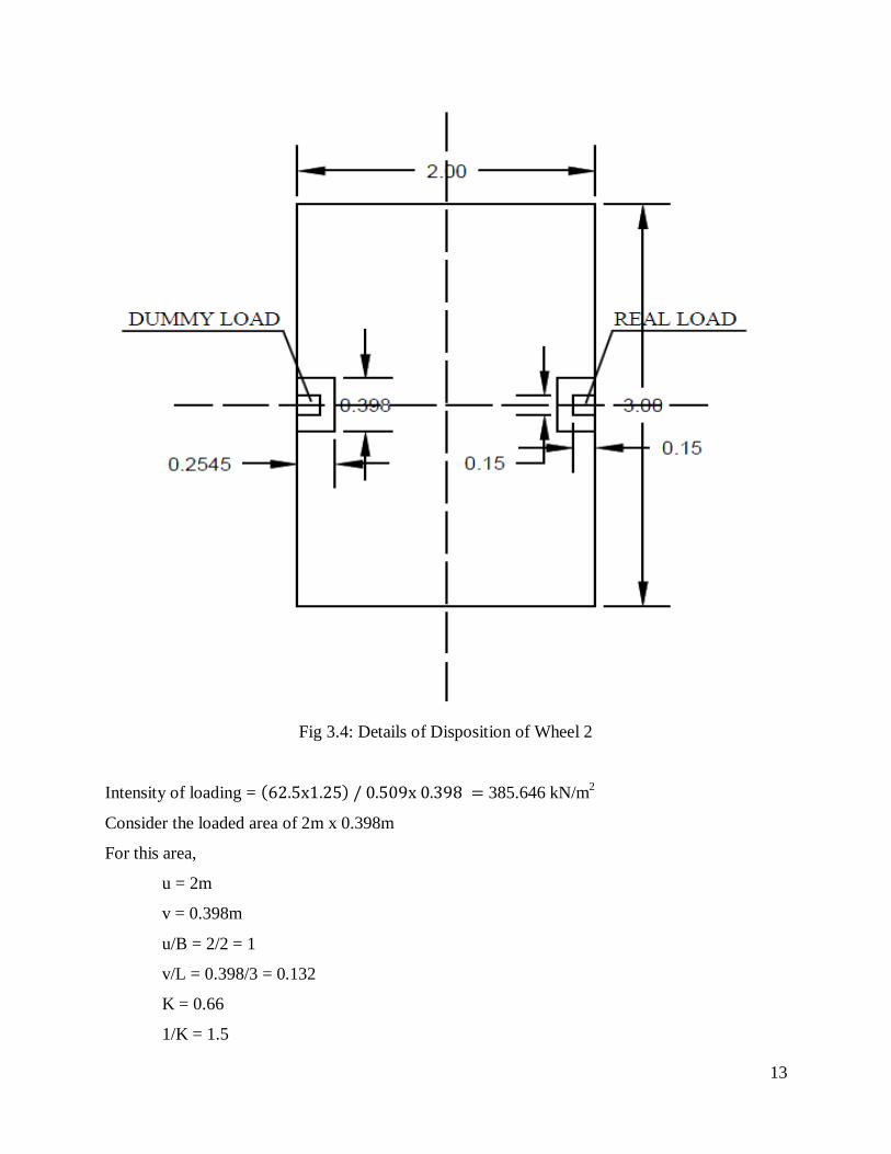
Fig 3.4: Details of Disposition of Wheel 2

Intensity of loading = 62.5x1.25 / 0.509x 0.398 = 385.646 kN/m2

Consider the loaded area of 2m x 0.398m

For this area,

u = 2m

v = 0.398m

u/B = 2/2 = 1

v/L = 0.398/3 = 0.132

K = 0.66

1/K = 1.5

14

Therefore,

m1 = 7.8x10-2

m2 = 8x10-2

Moment along short span = W (m1+ 0.15m2) = 385.646 (7.8 + (0.15x8)10-2

) x 2 x 0.398

= 27.63 kNm

Moment along long span = W (m2 + 0.15m1) = 385.646 (8 + (0.15x7.8) x 10-2

) x 2 x 0.398

= 28.15 kNm

Next, consider the area between the real load and the dummy load

i.e., 1.491 m x 0.398 m

For this moment,

u = 1.491m

v = 0.398m

u/B = 1.491/2 = 0.745

v/L = 0.398/3 = 0.132

Therefore,

m1 = 10.3x10-2

m2 = 10.2x10-2

Moment along short span = 385.646 [10.3 + (0.15 x 10.2) x 10-2

)] x 1.491 x 0.398 = 27.07 kNm

Moment along long span = 385.646 [10.2 + (0.15 x 10.3) x 10-2

] x 1.491 x 0.398 = 26.878 kNm

Net bending moment along short span = ½ [27.63-27.07] = 0.28 kNm

Net bending moment along long span = ½ [28.15-26.878] = 0.636 kNm

By similar figure and procedure for case (b), remaining cases are done.

(c) B.M. due to wheel 3

Intensity of loading = (37.5 x 1.25)/(0.509 x 0.398) = 231.387 kN/m2


For this area,

Moment along shorter span = 231.387 x [7.8 + (0.15 x 8) x 10-2

] x 2 x 0.398

= 16.576 kNm

Moment along longer span = 231.387 x [8 + (0.15 x 7.8) x 10-2

] x 2 x 0.398

= 16.89 kNm

15

The area between the real and the dummy load is 0.691m x 0.398m

u = 0.691

v = 0.398

u/B = 0.691/2 = 0.345

v/L = 0.398/3 = 0.132

Therefore,

m1 = 16.9 x 10-2

m2 = 14 x 10-2

Bending moment along shorter span = 231.387 x [16.9 + (0.15x14) x 10-2

] x 0.691 x 0.398

=12.1 kNm

Bending moment along longer span = 231.387 x [14 + (0.15x16.9) x 10-2

] x 0.691 x 0.398

= 10.52 kNm

Therefore,

Net bending moment along shorter span = ½ (16.576-12.1) = 2.238 kNm

Net bending moment along longer span = ½ (16.89-10.52) = 3.185 kNm

(d) B.M due to wheel 4

Here the load is placed eccentric with respect to the XX axis.

Intensity of loading = 385.646 kN/m2

The loaded area with respect to XX axis = 2m x 0.398m

Moment along shorter span = 27.63 kNm

Moment along longer span = 28.15 kNm

Consider the area between the real load and the dummy load = 0.509m x 0.802m

u = 0.509

v = 0.802

u/B = 0.509/2 = 0.25

v/L = 0.802/3 = 0.267

Therefore,

m1 = 17.8 x 10-2

m2 = 11 x 10-2

16


] x 0.509 x 0.802

= 30.62 kNm


] x 0.509 x 0.802

= 21.52 kNm

Therefore,

Net bending moment along shorter span = ½ (27.63-30.62) = -1.5 kNm


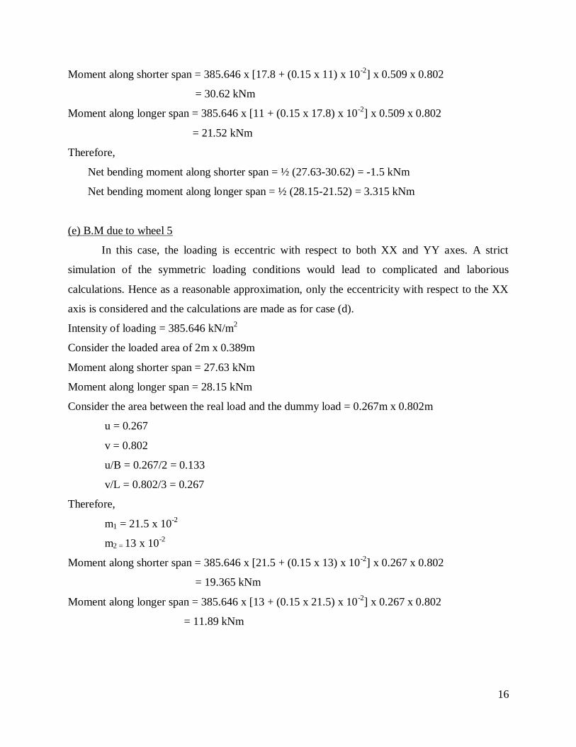
(e) B.M due to wheel 5

In this case, the loading is eccentric with respect to both XX and YY axes. A strict

simulation of the symmetric loading conditions would lead to complicated and laborious

calculations. Hence as a reasonable approximation, only the eccentricity with respect to the XX

axis is considered and the calculations are made as for case (d).






u = 0.267

v = 0.802

u/B = 0.267/2 = 0.133

v/L = 0.802/3 = 0.267

Therefore,

m1 = 21.5 x 10-2

m2 = 13 x 10-2


] x 0.267 x 0.802

= 19.365 kNm


] x 0.267 x 0.802

= 11.89 kNm

17

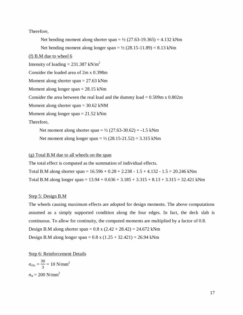
Therefore,

Net bending moment along shorter span = ½ (27.63-19.365) = 4.132 kNm


(f) B.M due to wheel 6






Moment along shorter span = 30.62 kNM


Therefore,

Net moment along shorter span = ½ (27.63-30.62) = -1.5 kNm

Net moment along longer span = ½ (28.15-21.52) = 3.315 kNm

(g) Total B.M due to all wheels on the span

The total effect is computed as the summation of individual effects.

Total B.M along shorter span = 16.596 + 0.28 + 2.238 - 1.5 + 4.132 - 1.5 = 20.246 kNm

Total B.M along longer span = 13.94 + 0.636 + 3.185 + 3.315 + 8.13 + 3.315 = 32.421 kNm

Step 5: Design B.M

The wheels causing maximum effects are adopted for design moments. The above computations

assumed as a simply supported condition along the four edges. In fact, the deck slab is

continuous. To allow for continuity, the computed moments are multiplied by a factor of 0.8.

Design B.M along shorter span = 0.8 x (2.42 + 28.42) = 24.672 kNm

Design B.M along longer span = 0.8 x (1.25 + 32.421) = 26.94 kNm

Step 6: Reinforcement Details

σcbc = 30

3 = 10 N/mm

2

σst = 200 N/mm2

18

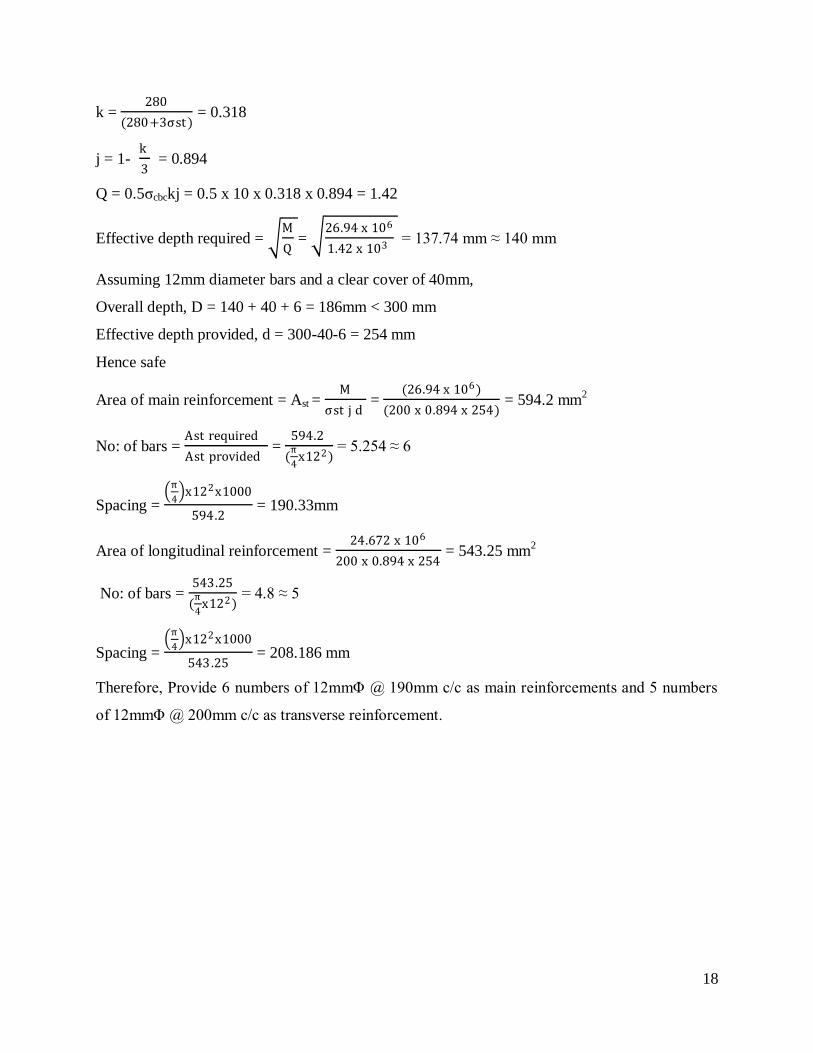
k = 280

(280+3σst ) = 0.318

j = 1- k

3 = 0.894

Q = 0.5σcbckj = 0.5 x 10 x 0.318 x 0.894 = 1.42

Effective depth required = M

Q =

26.94 x 106

1.42 x 103 = 137.74 mm ≈ 140 mm

Assuming 12mm diameter bars and a clear cover of 40mm,

Overall depth, D = 140 + 40 + 6 = 186mm < 300 mm

Effective depth provided, d = 300-40-6 = 254 mm

Hence safe

Area of main reinforcement = Ast = M

σst j d =

(26.94 x 106)

(200 x 0.894 x 254) = 594.2 mm

2

No: of bars = Ast required

Ast provided =

594.2

(π

4x122)

= 5.254 ≈ 6

Spacing = π

4 x122x1000

594.2 = 190.33mm

Area of longitudinal reinforcement = 24.672 x 106

200 x 0.894 x 254 = 543.25 mm

2

No: of bars = 543.25

(π

4x122)

= 4.8 ≈ 5

Spacing = π

4 x122x1000

543.25 = 208.186 mm

Therefore, Provide 6 numbers of 12mmΦ @ 190mm c/c as main reinforcements and 5 numbers

of 12mmΦ @ 200mm c/c as transverse reinforcement.

19

3.3. CANTILEVER SLAB

Step 1: Moment due to dead load

The total maximum moment due to dead load per metre width of cantilever slab is computed as

in the following table; using details from Fig 3.6.

Fig 3.5: Cantilever Slab with Class A wheel

Table 3.1: Dead load Calculation of Cantilever Slab

Sl.No Description Load (kN) Lever arm Moment (kNm)

1.

2.

3.

4.

5.

Handrails

Kerb

Footpath

Slab

rectangular

Slab

triangular

0.550 x (0.995+0.475)

x 24 = 19.4

0.225x0.225x24 = 1.215

1.475x0.275x24 = 9.735

2.25x0.2x24 = 2.7

0.5x2.25x0.05x24 = 1.35

0.550/2 = 0.275

[0.55+1.475+(0.225/2)]= 2.1375

[0.55+(1.475/2)] = 1.2875

2.25/2 = 1.125

2.25/3 = 0.75

5.34

2.6

12.53

3.04

1.0125

Total 51.88

20

Step 2: Moment due to live load

Live load on footpath = 400kg/m2 = 4kN/m

2 (From IRC 6: 2014)

Live load per meter width including impact = 4 x1.25 = 5 kN/m2

Moment due to live load = 5 x 1.475 x (1.475/8) = 1.36 kNm

Step 3: Reinforcement

Total moment due to dead load and live load = 51.88 + 1.36 = 53.24 kNm

Effective depth required = M

Q =

53.24 x 106

1.42 x 103 = 193.63 ≈ 200mm

Effective depth provided = 300 - 40 – 8 = 252 mm

Hence safe

Area of reinforcement required = Ast = M

σst j d =

(53.24 x 106)

(200 x 0.894 x 252) = 1181.59 mm

2

Adopt 16mmΦ bars as main reinforcements,


Ast provided =

1181.59

(π

4x162)

=5.87 ≈ 6

Spacing = π

4 x 162 x 1000

1181 .59 = 170.162mm

Therefore, provide 6 numbers of 16mmΦ @ 170mm c/c as main reinforcements.

B.M for distributors = 0.2 x 51.88 + 0.3 x 1.36 = 10.784 kNm

Area of distributors = 10.784 x 106

200 x 0.89 x 252 = 240.41 mm

2

Assuming 12mmΦ bars as distributors


Ast provided =

240.41

π

4x122

= 2.2 ≈ 4

Spacing = π

4 x 122 x 1000

240.41 = 170.162mm = 470.96mm

Therefore, provide 4 numbers of 12mmΦ @ 450mm c/c as distributors.

21

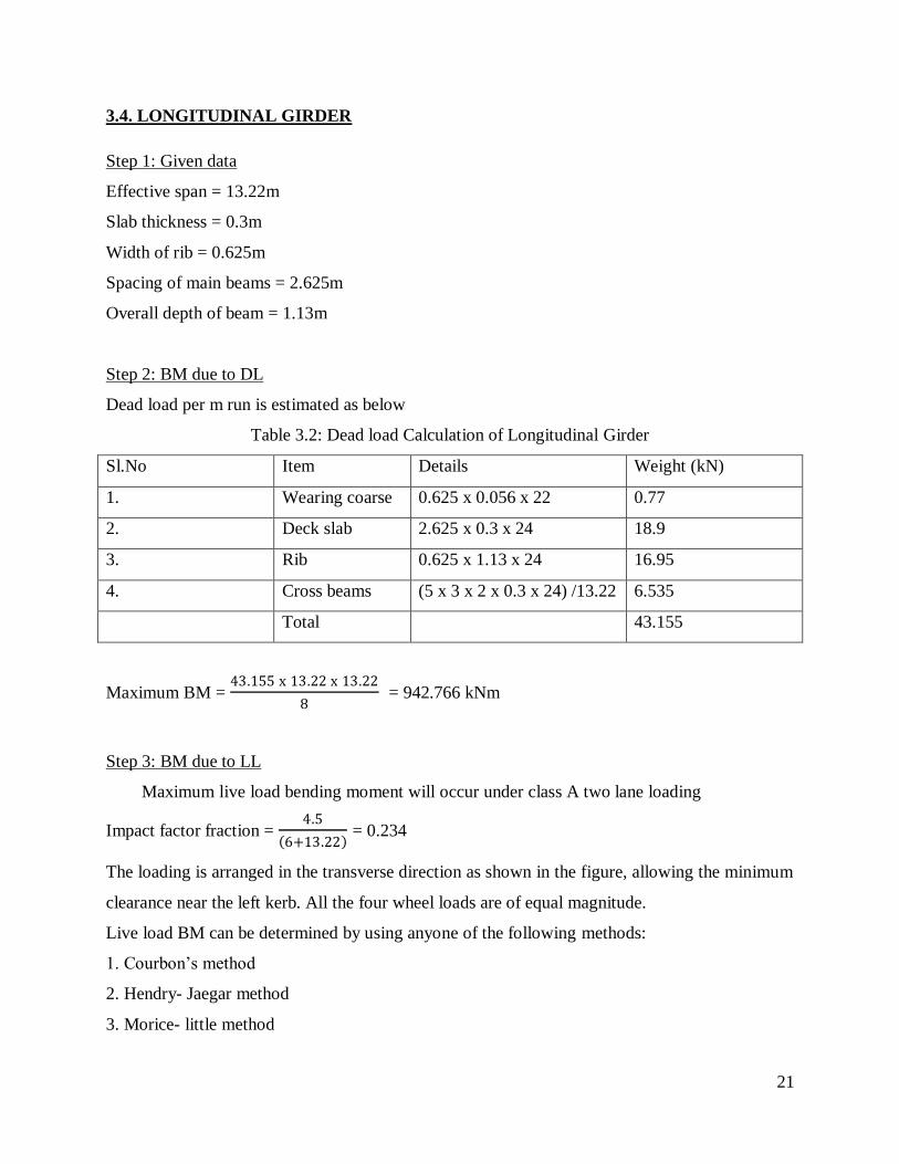
3.4. LONGITUDINAL GIRDER

Step 1: Given data

Effective span = 13.22m

Slab thickness = 0.3m

Width of rib = 0.625m

Spacing of main beams = 2.625m

Overall depth of beam = 1.13m

Step 2: BM due to DL

Dead load per m run is estimated as below

Table 3.2: Dead load Calculation of Longitudinal Girder

Sl.No Item Details Weight (kN)

1. Wearing coarse 0.625 x 0.056 x 22 0.77

2. Deck slab 2.625 x 0.3 x 24 18.9

3. Rib 0.625 x 1.13 x 24 16.95

4. Cross beams (5 x 3 x 2 x 0.3 x 24) /13.22 6.535

Total 43.155

Maximum BM = 43.155 x 13.22 x 13.22

8 = 942.766 kNm

Step 3: BM due to LL

Maximum live load bending moment will occur under class A two lane loading

Impact factor fraction = 4.5

6+13.22 = 0.234

The loading is arranged in the transverse direction as shown in the figure, allowing the minimum

clearance near the left kerb. All the four wheel loads are of equal magnitude.

Live load BM can be determined by using anyone of the following methods:

1. Courbon‘s method

2. Hendry- Jaegar method

3. Morice- little method

22

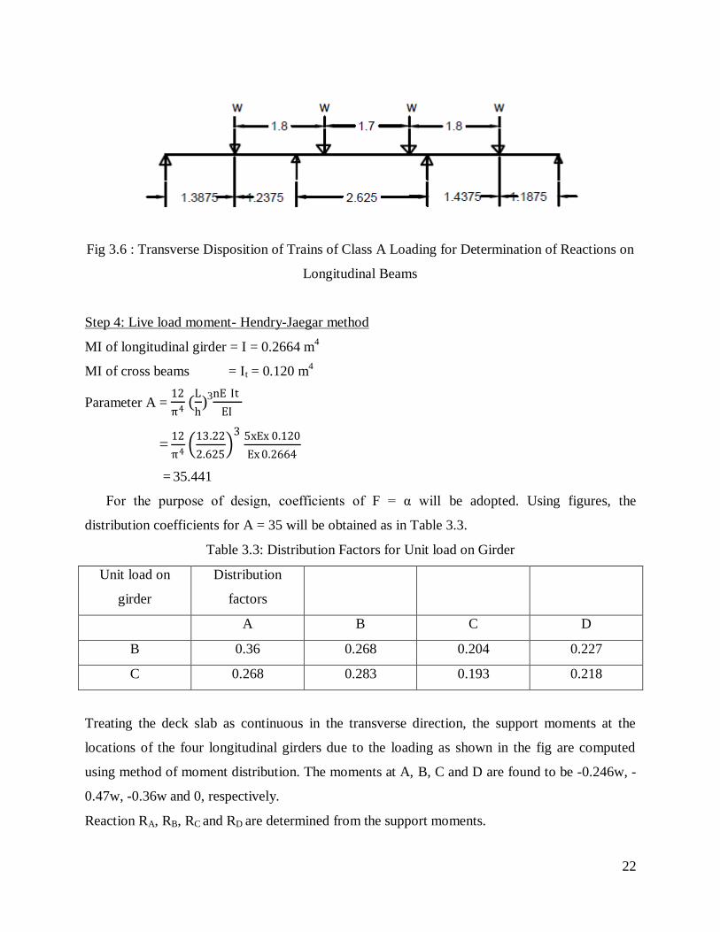
Fig 3.6 : Transverse Disposition of Trains of Class A Loading for Determination of Reactions on

Longitudinal Beams

Step 4: Live load moment- Hendry-Jaegar method

MI of longitudinal girder = I = 0.2664 m4

MI of cross beams = It = 0.120 m4

Parameter A = 12

π4(

L

h)

3nE It

EI

= 12

π4

13.22

2.625

3 5xEx 0.120

Ex 0.2664

= 35.441

For the purpose of design, coefficients of F = α will be adopted. Using figures, the

distribution coefficients for A = 35 will be obtained as in Table 3.3.

Table 3.3: Distribution Factors for Unit load on Girder

Unit load on

girder

Distribution

factors

A B C D

B 0.36 0.268 0.204 0.227

C 0.268 0.283 0.193 0.218

Treating the deck slab as continuous in the transverse direction, the support moments at the

locations of the four longitudinal girders due to the loading as shown in the fig are computed

using method of moment distribution. The moments at A, B, C and D are found to be -0.246w, -

0.47w, -0.36w and 0, respectively.

Reaction RA, RB, RC and RD are determined from the support moments.

23

RA = 0.471w

RB = 1.45w

RC = 1.53w

RD = 0.55w

These reactions are treated as loads on the interconnected girder system and multiplying these

by the respective distribution coefficients and adding the results under each girder and the final

reaction at each girder is obtained as shown in the table

Maximum bending moment on the intermediate beam = 952 kNm

Table 3.4: Reaction Factors on Girder

Load Girder A Girder B Girder C Girder D

1) 1.45w on

girder B

0.36x1.45w

= 0.522w

0.268x1.45w

= 0.3886w

0.204x1.45w

= 0.3w

0.227x1.45w

= 0.33w

2) 1.53w on

Girder C

0.268x1.53w

= 0.41w

0.283x1.53w

= 0.433w

0.193x1.53w

= 0.295w

0.218x1.53w

= 0.33w

Net reaction 0.932w 0.822w 0.6w 0.66w

Step 6: Design maximum bending moment

Live load bending moment obtained from Hendry Jaegar method will be adopted as

Design B.M = Moment due to D.L + Moment due to L.L

= 942.766 + 952 = 1894.766 kNm

≈ 1900 kNm

Step 7: Design of section

Effective flange width for the Tee beam section will be determined as er clause 305.15.2 of IRC

Bridge code.

24

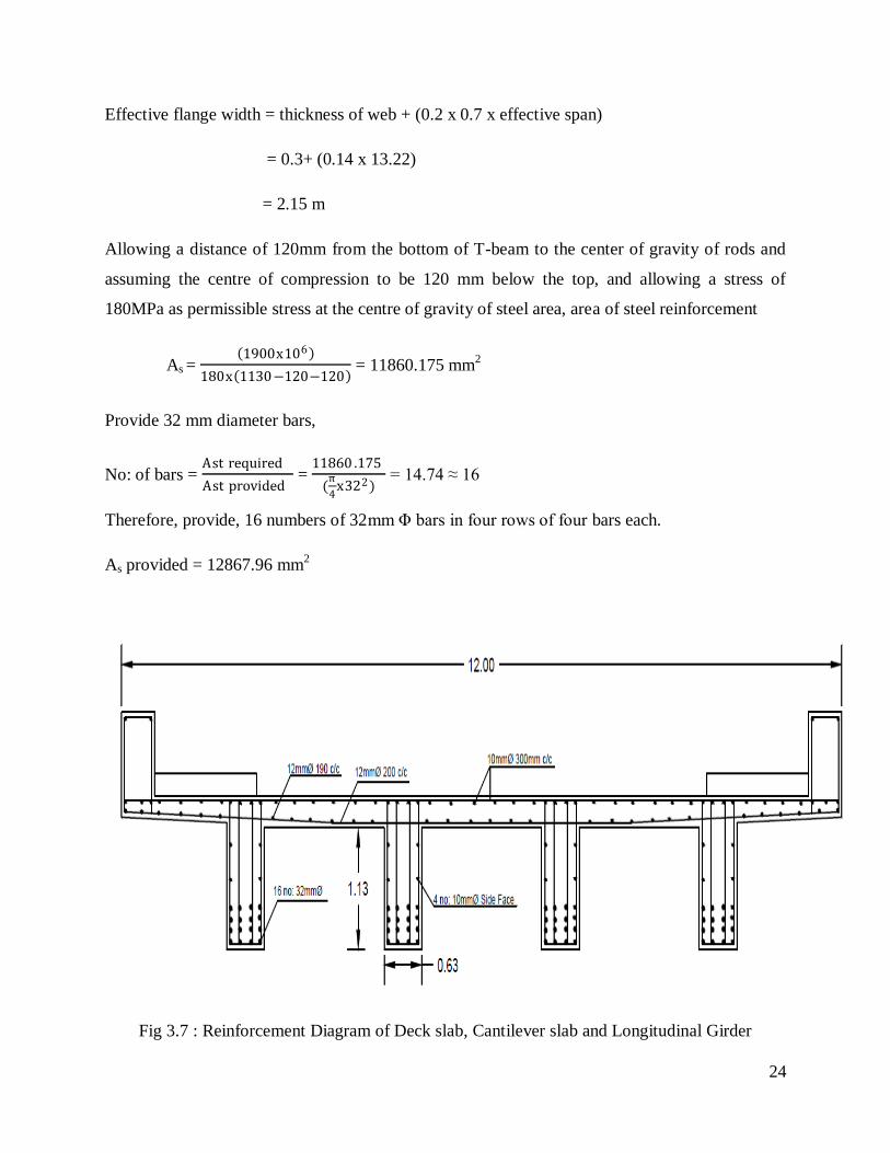
Effective flange width = thickness of web + (0.2 x 0.7 x effective span)

= 0.3+ (0.14 x 13.22)

= 2.15 m

Allowing a distance of 120mm from the bottom of T-beam to the center of gravity of rods and

assuming the centre of compression to be 120 mm below the top, and allowing a stress of

180MPa as permissible stress at the centre of gravity of steel area, area of steel reinforcement

As = 1900x106

180x 1130−120−120 = 11860.175 mm

2

Provide 32 mm diameter bars,


Ast provided =

11860 .175

(π

4x322)

= 14.74 ≈ 16

Therefore, provide, 16 numbers of 32mm Φ bars in four rows of four bars each.

As provided = 12867.96 mm2

Fig 3.7 : Reinforcement Diagram of Deck slab, Cantilever slab and Longitudinal Girder

25

3.5. CROSS GIRDER

Step 1: Given data

Spacing of cross beam = 3m

Effective span = 2.625 - 0.625 = 2 m

Impact factor for 2 m span for

Class AA tracked vehicle = 0.25

Class AA wheeled vehicle = 0.25

Class A loading = 0.55

Step 2: BM due to DL

The weight of slab and wearing course will be apportioned between the cross beams and the

longitudinal girders in accordance with the trapezoidal distribution of the loads on the panel as

shown in Fig 3.10

Fig 3.8: Deck Panel showing Trapezoidal Distribution of Dead Load

26

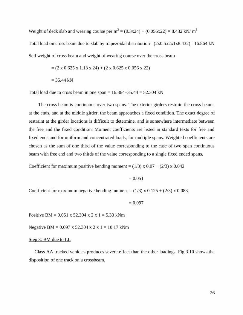
Weight of deck slab and wearing course per m2 = (0.3x24) + (0.056x22) = 8.432 kN/ m

2

Total load on cross beam due to slab by trapezoidal distribution= (2x0.5x2x1x8.432) =16.864 kN

Self weight of cross beam and weight of wearing course over the cross beam

= (2 x 0.625 x 1.13 x 24) + (2 x 0.625 x 0.056 x 22)

= 35.44 kN

Total load due to cross beam in one span = 16.864+35.44 = 52.304 kN

The cross beam is continuous over two spans. The exterior girders restrain the cross beams

at the ends, and at the middle girder, the beam approaches a fixed condition. The exact degree of

restraint at the girder locations is difficult to determine, and is somewhere intermediate between

the free and the fixed condition. Moment coefficients are listed in standard texts for free and

fixed ends and for uniform and concentrated loads, for multiple spans. Weighted coefficients are

chosen as the sum of one third of the value corresponding to the case of two span continuous

beam with free end and two thirds of the value corresponding to a single fixed ended spans.

Coefficient for maximum positive bending moment = (1/3) x 0.07 + (2/3) x 0.042

= 0.051

Coefficient for maximum negative bending moment = (1/3) x 0.125 + (2/3) x 0.083

= 0.097

Positive BM = 0.051 x 52.304 x 2 x 1 = 5.33 kNm

Negative BM = 0.097 x 52.304 x 2 x 1 = 10.17 kNm

Step 3: BM due to LL

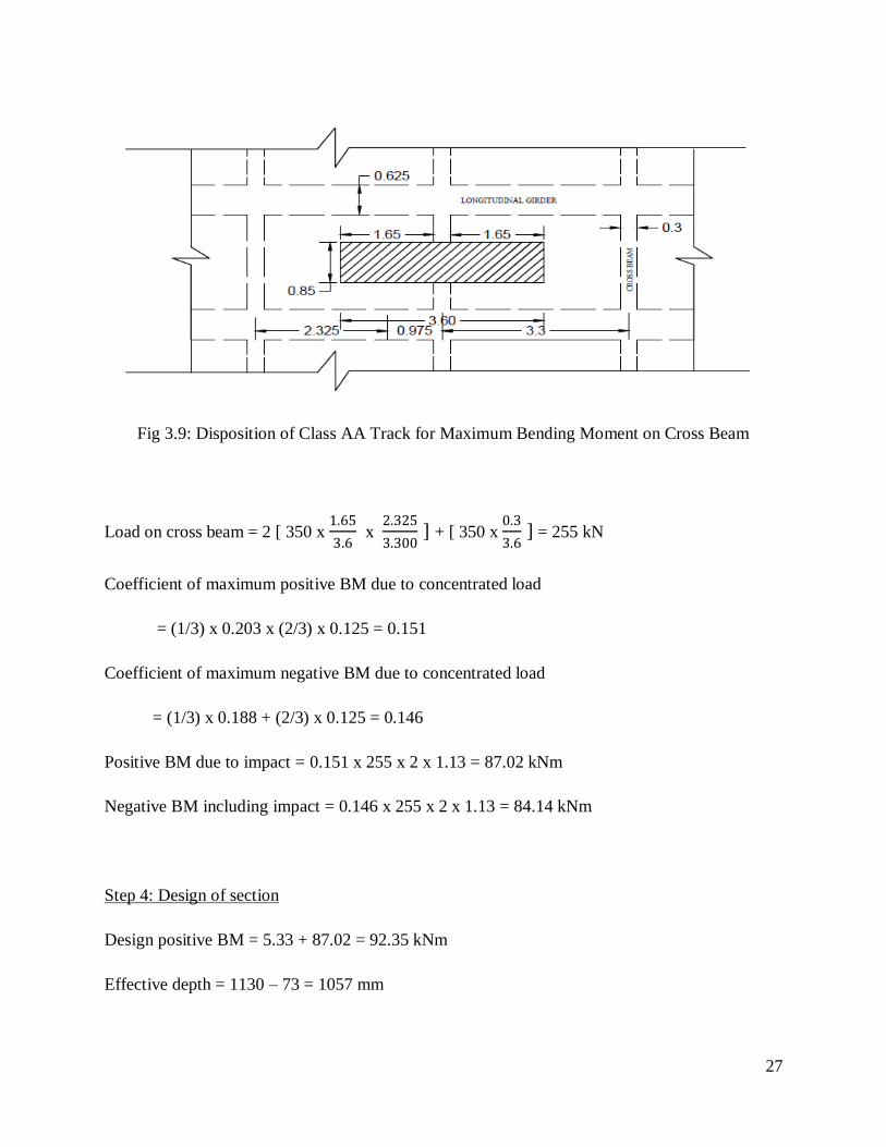
Class AA tracked vehicles produces severe effect than the other loadings. Fig 3.10 shows the

disposition of one track on a crossbeam.

27

Fig 3.9: Disposition of Class AA Track for Maximum Bending Moment on Cross Beam

Load on cross beam = 2 [ 350 x 1.65

3.6 x

2.325

3.300 ] + [ 350 x

0.3

3.6 ] = 255 kN

Coefficient of maximum positive BM due to concentrated load

= (1/3) x 0.203 x (2/3) x 0.125 = 0.151

Coefficient of maximum negative BM due to concentrated load

= (1/3) x 0.188 + (2/3) x 0.125 = 0.146

Positive BM due to impact = 0.151 x 255 x 2 x 1.13 = 87.02 kNm

Negative BM including impact = 0.146 x 255 x 2 x 1.13 = 84.14 kNm

Step 4: Design of section

Design positive BM = 5.33 + 87.02 = 92.35 kNm

Effective depth = 1130 – 73 = 1057 mm

28

Area of steel required = (92.35 x 106)

(200 x 0.89 x 1057) = 490.84 mm

2

Add 0.3% of area of the beam to give additional stiffness to the beam

Additional area of steel required = (0.3/100) x 200 x 1057 =634.2 mm2

Total area of steel required = 490.84 + 634.2 = 1125.04mm2

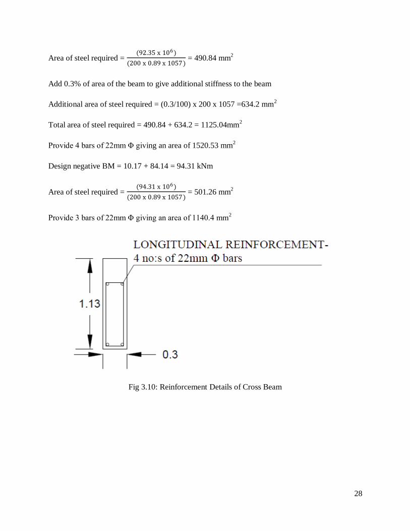
Provide 4 bars of 22mm Φ giving an area of 1520.53 mm2

Design negative BM = 10.17 + 84.14 = 94.31 kNm

Area of steel required = (94.31 x 106)

(200 x 0.89 x 1057) = 501.26 mm

2

Provide 3 bars of 22mm Φ giving an area of 1140.4 mm2

Fig 3.10: Reinforcement Details of Cross Beam

29

3.6. BEARINGS

Design an elastomeric unreinforced neoprene pad bearing to suit the following data.

Vertical DL = 877.34 + 68.8 = 946.14 ≈ 1000 kN

Vertical LL = 700 kN

Horizontal force = 0.2 x 700 = 140 kN

Modulus of rigidity of elastomer = G = 1 N/mm2

Friction coefficient = 0.3

Step 1: Design

Total vertical load = 1000+700 = 1700 kN

Horizontal force = 140 kN

From IRC: 83 1987, Part II,

Select the standard plan dimensions of elastomeric bearings,

a = 350 mm

b = 700 mm

Thickness, (t) should be less than a/5

Therefore, select a thickness of 50 mm

Area, A = 350 x 700 = 245000 mm2

tanΦ = H

GA =

140 x 103

1 x 245000 = 0.571

u = t tanΦ = 50 x 0.571 = 28.55

But t >1.43u

30

1.43 u = 1.43 x 28.55 = 40.82 < 50 mm

Hence design is safe.

Step 2: Axial stress

Shape factor = S = ab

2t(a+b) =

350 x 700

2 x 50 (350+700) = 2.33

σm = P

A1

P = 1000 kN

A1 = (a-u)b = (350 – 28.55) x 700 = 225015 mm

2

σm = 1000 x 103

225015 = 4.44

Check:

σm < 2GS

2GS = 2 x 1 x 2.33 =4.66

4.44 < 4.66

Hence design is safe

σm1 =

PL

A1 =

700 x 103

225015 = 3.11 > 1 +

a

b = 1+

350

700 = 1.5

3.11 > 1.5

Hence design is safe

31

3.7. PEDESTALS

Step 1: Given Details

Total factored load = 3100 kN

Size of base plate = 300mm x 300mm

M30 concrete and Fe415 steel

Step 2: Design

Adopt minimum size of pedestal including 10mm clearance = (size of base plate + clearance)2

= 310mm x 310mm

Safe pressure = bearing strength x 310/300

Bearing strength = fcb = 0.45fck = 0.45x30 = 13.5 N/mm2

Therefore, safe pressure = 13.5 x (310/300) = 13.95 N/mm2

Load carried by pedestal = 13.95 x 310 x 310 = 1340.595 kN

Balance load = 3100 – 1340.595 = 1759.405 ≈ 1760 kN

Area of reinforcements required = (1760 x 10−3)

(0.87 x 415) = 4874.67 mm

2

Assume 24 mm diameter bars,


Ast provided =

4874.67

(π

4x242)

= 10.77 ≈ 12

Spacing = π

4 x242x1000

4874 .67 = 92.8 mm

Provide 6 nos of 24 mm diameter on both sides of the base plate at 90mm c/c

Step 3: Check for percentage steel

% of steel = 4874.67

(310x310)x 100 = 5.07 > 0.4 % , Hence safe

32

3.8. OPERATING PLATFORM

Step 1: Given details

Span = 13.22m

M30 grade concrete

Fe415 grade steel

Total load acting on the operating platform, W = 20 Tonne = 20 x 10 = 200 kN

Therefore, load acting on each beam = 200

2 x 13.22 = 7.56 kN/m

Assume, b/d = 0.5

Step 2: Moment of resistance

Mr = Qbd2

Q = 0.5σcbckj

σcbc = 30

3 = 10 N/mm

2

k = 280

(280+3σst ) = 0.318

j = 1-𝑘

3 = 0.894

Q = 0.5σcbckj = 0.5 x 10 x 0.318 x 0.894 = 1.42

Mr = 1.42 x 0.5d x d2

= 0.71d3

Step 3: Moment calculation

M = W L2

8 =

7.56 x 13.222

8 = 165.156 kNm

33

M = Mr

165.156 x 106 = 0.71d

3

Therefore, d = 615.005 mm = 615mm

b = 0.5d = 0.5 x 615 = 307.5mm

Therefore, adopt dimensions of the beam = 0.31m x 0.62m

Step 4: Reinforcement Details

Ast = M

σst j d =

165.156 x 106

(200 x 0.894 x 620 = 1489.82 mm

2

Adopt 16mmΦ bars,


Ast provided =

1489.82

(π

4x162)

= 7.41 ≈ 8

Spacing = π

4 x162x1000

1489.82 = 134.95mm

Therefore, provide 6 numbers of 16mmΦ @ 130mm c/c.

Ast provided = 6 x (π/4) x 162 = 1206.37 mm

2

Ast remaining = 1489.82-1206.37 = 283.448 mm2

Provide 2 legged 8mm diameter vertical stirrups,

No: of stirrups = 283.448/((π/4) x 82) = 5.64

Therefore, provide 6 nos of 8mmΦ 2 legged vertical stirrups.

34

3.9. PIER

Step 1: Given details

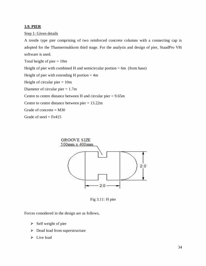
A trestle type pier comprising of two reinforced concrete columns with a connecting cap is

adopted for the Thannermukkom third stage. For the analysis and design of pier, StaadPro V8i

software is used.

Total height of pier = 10m

Height of pier with combined H and semicircular portion = 6m (from base)

Height of pier with extending H portion = 4m

Height of circular pier = 10m

Diameter of circular pier = 1.7m

Centre to centre distance between H and circular pier = 9.65m

Centre to centre distance between pier = 13.22m

Grade of concrete = M30

Grade of steel = Fe415

Fig 3.11: H pier

Forces considered in the design are as follows,

Self weight of pier

Dead load from superstructure

Live load

35

Impact allowance

Load from operating platform

Water pressure on pier

Force on pier due to water pressure from submerged shutter

Breaking force

Wind load

Effect of buoyancy

Step 2: Calculation of design loads

(a) Self weight of pier

StaadPro generates the self weight based on model created.

(b) Dead load from superstructure

Total load including self weight of deck slab, girders, wearing course, parapet =157 KN/m.

This load is equally distributed over 4 main girders.

Load per girder= 39.25 KN/m

(c) Live load

As per IRC 6-2000, clause 207.4 Table 2

2 lanes of class A loading.

(d)Impact Allowance

IRC 6-2000 clause 211.1

Impact factor fraction = 4.5

6+13.22 = 0.234

Impact Factor = 0.234

This fraction of live load has been given as impact allowance.

36

(e) Load from operating platform

Load from operating platform = 70.06 KN on each pier

(f) Water pressure on pier

IRC 6-2000 clause 213.1

P= 0.5 KV2

K=0.66 For piers with semicircular ends

V= 3 m/s

Water pressure = 32.67 kN

(g) Water pressure-submerged shutter

Water pressure from submerged shutter= 235.44 KN

(h)Breaking Force

IRC 6-2000 clause 214.2, 20% of vehicular load is taken.

20% of class AA load = 0.2 x 700 = 140KN

(h) Effect of Buoyancy

The upward force is equal to the weight of water displaced by the submerged body.

Submerged volume of H pier= 6.74 x 5.5 =37.07m3

Unit weight of water = 10KN/m

3

Buoyant force = 370.7 KN

Submerged volume of circular pier =12.48 m3

Buoyant force = 124.8 KN

37

(i) Wind load

IRC 6-2000 clause 212.3

Wind load = Area of exposure x wind intensity

Total wind load = 44.1 KN

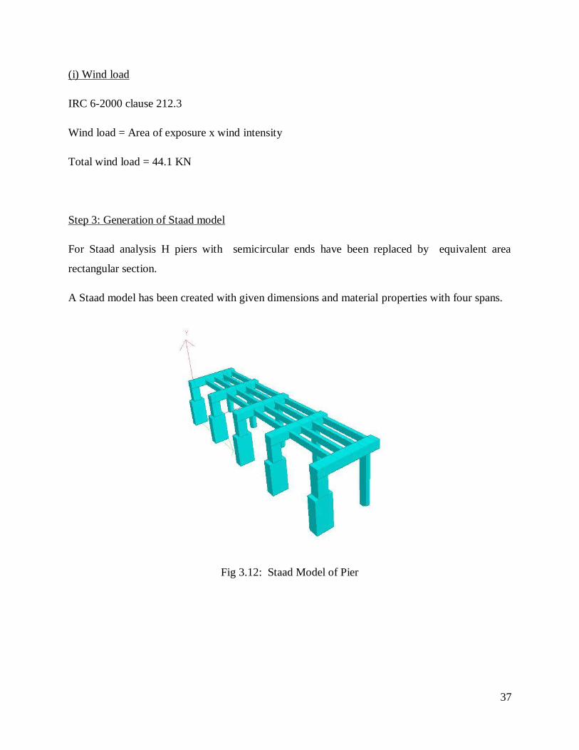
Step 3: Generation of Staad model

For Staad analysis H piers with semicircular ends have been replaced by equivalent area

rectangular section.

A Staad model has been created with given dimensions and material properties with four spans.

Fig 3.12: Staad Model of Pier

38

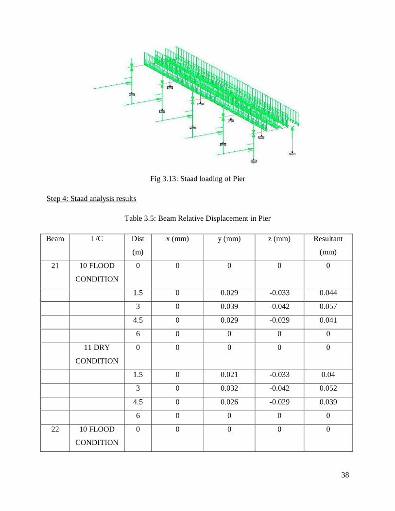
Fig 3.13: Staad loading of Pier

Step 4: Staad analysis results

Table 3.5: Beam Relative Displacement in Pier

Beam L/C Dist

(m)

x (mm) y (mm) z (mm) Resultant

(mm)

21 10 FLOOD

CONDITION

0 0 0 0 0

1.5 0 0.029 -0.033 0.044

3 0 0.039 -0.042 0.057

4.5 0 0.029 -0.029 0.041

6 0 0 0 0

11 DRY

CONDITION

0 0 0 0 0

1.5 0 0.021 -0.033 0.04

3 0 0.032 -0.042 0.052

4.5 0 0.026 -0.029 0.039

6 0 0 0 0

22 10 FLOOD

CONDITION

0 0 0 0 0

39

1 0 0.117 -0.005 0.117

2 0 0.163 -0.008 0.163

3 0 0.127 -0.004 0.127

4 0 0 0 0

11 DRY

CONDITION

0 0 0 0 0

1 0 0.12 -0.005 0.12

2 0 0.166 -0.008 0.166

3 0 0.129 -0.004 0.13

4 0 0 0 0

30 10 FLOOD

CONDITION

0 0 0 0 0

2.5 0 0.537 -0.017 0.538

5 0 0.415 -0.112 0.43

7.5 0 0.084 -0.15 0.172

10 0 0 0 0

11 DRY

CONDITION

0 0 0 0 0

2.5 0 0.537 -0.017 0.537

5 0 0.422 -0.112 0.437

7.5 0 0.097 -0.15 0.179

10 0 0 0 0

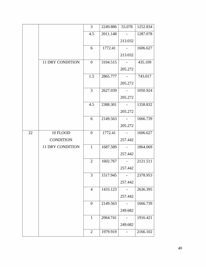
Table 3.6: Axial force – Shear force – Bending moment in Pier

Beam L/C Dist

(m)

Fx (kN) Fy (kN) Mz

(kNm)

21 10 FLOOD

CONDITION

0 2727.363 55.078 1418.068

1.5 2488.624 55.078 1335.451

40

3 2249.886 55.078 1252.834

4.5 2011.148 -

213.032

1287.078

6 1772.41 -

213.032

1606.627

11 DRY CONDITION 0 3104.515 -

205.272

435.109

1.5 2865.777 -

205.272

743.017

3 2627.039 -

205.272

1050.924

4.5 2388.301 -

205.272

1358.832

6 2149.563 -

205.272

1666.739

22 10 FLOOD

CONDITION

11 DRY CONDITION

0 1772.41 -

257.442

1606.627

1 1687.589 -

257.442

1864.069

2 1602.767 -

257.442

2121.511

3 1517.945 -

257.442

2378.953

4 1433.123 -

257.442

2636.395

0 2149.563 -

249.682

1666.739

1 2064.741 -

249.682

1916.421

2 1979.919 - 2166.102

41

249.682

3 1895.098 -

249.682

2415.784

4 1810.276 -

249.682

2665.466

30 10 FLOOD

CONDITION

0 3241.637 258.347 1587.142

2.5 3375.337 258.347 941.274

5 3509.038 258.347 295.407

7.5 3642.738 258.347 -350.46

10 3776.438 258.347 -996.328

11 DRY CONDITION 0 3359.985 250.586 1553.945

2.5 3493.685 250.586 927.479

5 3627.385 250.586 301.013

7.5 3761.085 250.586 -325.453

10 3894.786 250.586 -951.919

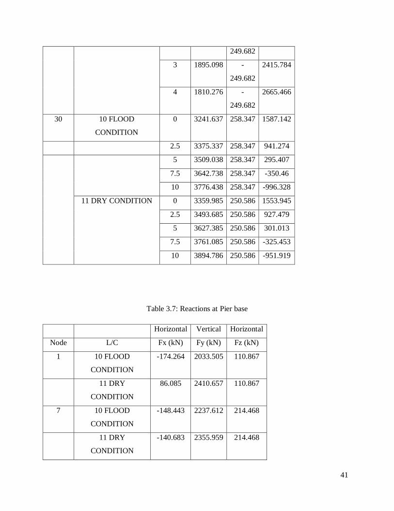
Table 3.7: Reactions at Pier base

Horizontal Vertical Horizontal

Node L/C Fx (kN) Fy (kN) Fz (kN)

1 10 FLOOD

CONDITION

-174.264 2033.505 110.867

11 DRY

CONDITION

86.085 2410.657 110.867

7 10 FLOOD

CONDITION

-148.443 2237.612 214.468

11 DRY

CONDITION

-140.683 2355.959 214.468

42

14 10 FLOOD

CONDITION

-47.768 2768.891 -106.321

11 DRY

CONDITION

212.582 3146.043 -106.321

20 10 FLOOD

CONDITION

-262.542 3895.047 -107.03

11 DRY

CONDITION

-254.781 4013.395 -107.03

25 10 FLOOD

CONDITION

-55.078 2727.363 -71.408

11 DRY

CONDITION

205.272 3104.515 -71.408

31 10 FLOOD

CONDITION

-258.347 3776.438 -75.393

11 DRY

CONDITION

-250.586 3894.786 -75.393

36 10 FLOOD

CONDITION

-48.007 2766.245 -38.282

11 DRY

CONDITION

212.342 3143.397 -38.282

42 10 FLOOD

CONDITION

-262.212 3886.525 -46.872

11 DRY

CONDITION

-254.452 4004.872 -46.872

47 10 FLOOD

CONDITION

-157.369 2052.713 -238.54

11 DRY

CONDITION

102.98 2429.866 -238.54

53 10 FLOOD

CONDITION

-148.57 2297.244 -341.489

43

11 DRY

CONDITION

-140.809 2415.591 -341.489

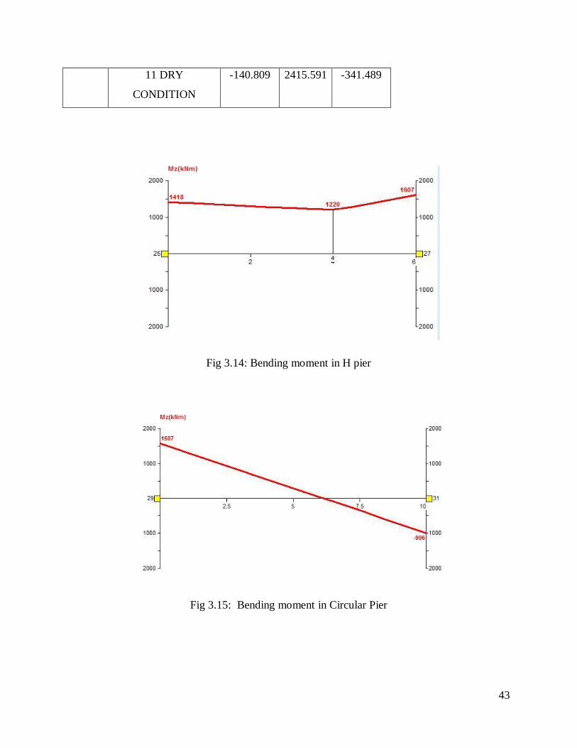
Fig 3.14: Bending moment in H pier

Fig 3.15: Bending moment in Circular Pier

44

Fig 3.16: Stress contour for H pier

Fig 3.17: Stress contour for Circular Pier

45

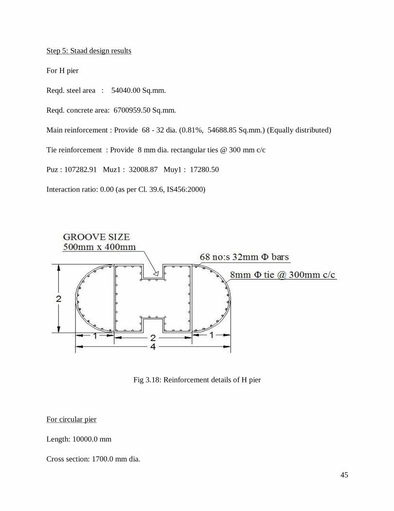
Step 5: Staad design results

For H pier

Reqd. steel area : 54040.00 Sq.mm.

Reqd. concrete area: 6700959.50 Sq.mm.

Main reinforcement : Provide 68 - 32 dia. (0.81%, 54688.85 Sq.mm.) (Equally distributed)

Tie reinforcement : Provide 8 mm dia. rectangular ties @ 300 mm c/c

Puz : 107282.91 Muz1 : 32008.87 Muy1 : 17280.50

Interaction ratio: 0.00 (as per Cl. 39.6, IS456:2000)

Fig 3.18: Reinforcement details of H pier

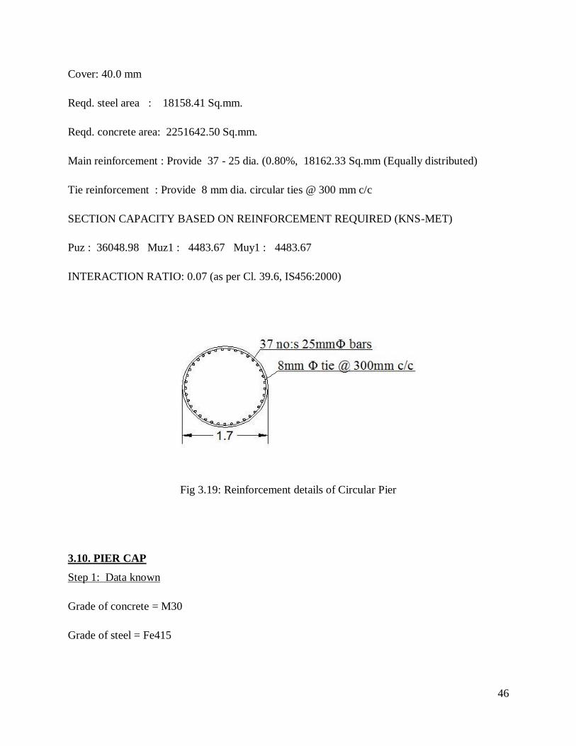
For circular pier

Length: 10000.0 mm

Cross section: 1700.0 mm dia.

46

Cover: 40.0 mm

Reqd. steel area : 18158.41 Sq.mm.

Reqd. concrete area: 2251642.50 Sq.mm.

Main reinforcement : Provide 37 - 25 dia. (0.80%, 18162.33 Sq.mm (Equally distributed)

Tie reinforcement : Provide 8 mm dia. circular ties @ 300 mm c/c

SECTION CAPACITY BASED ON REINFORCEMENT REQUIRED (KNS-MET)

Puz : 36048.98 Muz1 : 4483.67 Muy1 : 4483.67

INTERACTION RATIO: 0.07 (as per Cl. 39.6, IS456:2000)

Fig 3.19: Reinforcement details of Circular Pier

3.10. PIER CAP

Step 1: Data known

Grade of concrete = M30

Grade of steel = Fe415

47

Fig 3.20: Pier Cap Plan

Design loads are as follows,

Superstructure dead load

Live load

Load from operating platform

Self weight

Load from deck slab

The superstructure dead load is equally shared by four girders

Dead load from superstructure = 626.44 KN per girder

Live load

As per IRC 6-2000, clause 207.4 Table 2

2 lanes of class A loading.

Analysis and design are performed in StaadPro V8i.

48

Step 2: Generation of Staad loading

Fig 3.21: Staad loading of Pier Cap

Step 3: Staad analysis results

Table 3.8: Beam Relative Displacement in Pier Cap

Beam L/C Dist

(m)

x

(mm)

y

(mm)

z

(mm)

Resultant

(mm)

31 5 COMBINATION LOAD

CASE 5

0 0 0 0 0

0.25 0 0 0 0

0.5 0 0 0 0

0.75 0 0 0 0

1 0 0 0 0


CASE 5

0 0 0 0 0

2.412 0 -0.928 0 0.928

4.825 0 -1.501 0 1.501

7.237 0 -1.032 0 1.032

9.65 0 0 0 0


CASE 5

0 0 0 0 0

0.588 0 0.007 0 0.007

49

1.175 0 0.006 0 0.006

1.763 0 0.003 0 0.003

2.35 0 0 0 0

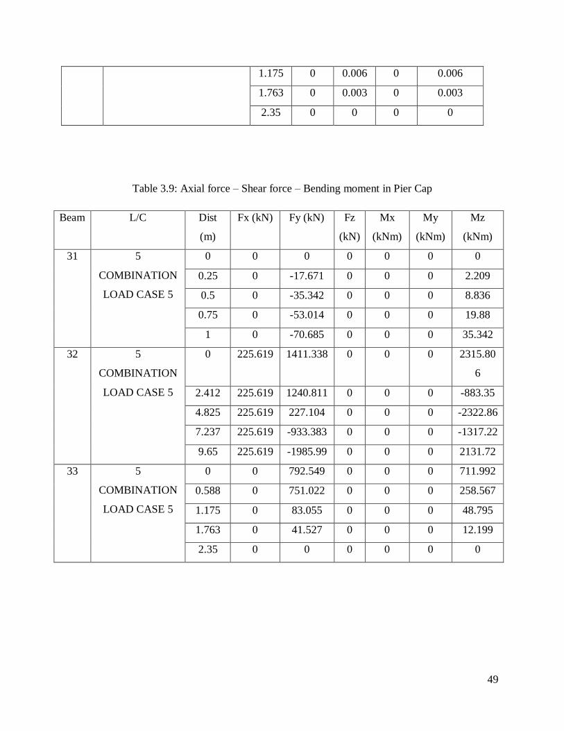
Table 3.9: Axial force – Shear force – Bending moment in Pier Cap

Beam L/C Dist

(m)

Fx (kN) Fy (kN) Fz

(kN)

Mx

(kNm)

My

(kNm)

Mz

(kNm)

31 5

COMBINATION

LOAD CASE 5

0 0 0 0 0 0 0

0.25 0 -17.671 0 0 0 2.209

0.5 0 -35.342 0 0 0 8.836

0.75 0 -53.014 0 0 0 19.88

1 0 -70.685 0 0 0 35.342

32 5

COMBINATION

LOAD CASE 5

0 225.619 1411.338 0 0 0 2315.80

6

2.412 225.619 1240.811 0 0 0 -883.35

4.825 225.619 227.104 0 0 0 -2322.86

7.237 225.619 -933.383 0 0 0 -1317.22

9.65 225.619 -1985.99 0 0 0 2131.72

33 5

COMBINATION

LOAD CASE 5

0 0 792.549 0 0 0 711.992

0.588 0 751.022 0 0 0 258.567

1.175 0 83.055 0 0 0 48.795

1.763 0 41.527 0 0 0 12.199

2.35 0 0 0 0 0 0

50

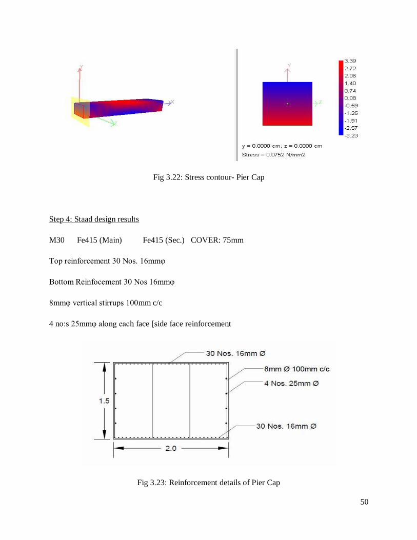
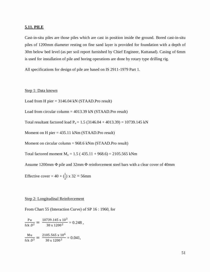
Fig 3.22: Stress contour- Pier Cap

Step 4: Staad design results

M30 Fe415 (Main) Fe415 (Sec.) COVER: 75mm

Top reinforcement 30 Nos. 16mmυ

Bottom Reinfocement 30 Nos 16mmυ

8mmυ vertical stirrups 100mm c/c

4 no:s 25mmυ along each face [side face reinforcement

Fig 3.23: Reinforcement details of Pier Cap

51

5.11. PILE

Cast-in-situ piles are those piles which are cast in position inside the ground. Bored cast-in-situ

piles of 1200mm diameter resting on fine sand layer is provided for foundation with a depth of

30m below bed level (as per soil report furnished by Chief Engineer, Kuttanad). Casing of 6mm

is used for installation of pile and boring operations are done by rotary type drilling rig.

All specifications for design of pile are based on IS 2911-1979 Part 1.

Step 1: Data known

Load from H pier = 3146.04 kN (STAAD.Pro result)

Load from circular column = 4013.39 kN (STAAD.Pro result)

Total resultant factored load Pu = 1.5 (3146.04 + 4013.39) = 10739.145 kN

Moment on H pier = 435.11 kNm (STAAD.Pro result)

Moment on circular column = 968.6 kNm (STAAD.Pro result)

Total factored moment Mu = 1.5 ( 435.11 + 968.6) = 2105.565 kNm

Assume 1200mm Φ pile and 32mm Φ reinforcement steel bars with a clear cover of 40mm

Effective cover = 40 + (1

2) x 32 = 56mm

Step 2: Longitudinal Reinforcement

From Chart 55 (Interaction Curve) of SP 16 : 1960, for

Pu

fck 𝐷2=

10739.145 x 103

30 x 12002 = 0.248 ,

Mu

fck 𝐷3=

2105.565 x 106

30 x 12003 = 0.041,

52

d′

D=

56

1200 = 0.046 ≈ 0.05 and

fy = 415N/mm2 ,

Percentage steel required for longitudinal reinforcement in piles ‗p‘ is given by P

fck = 0.02

p = 0.02 x 30 = 0.6%

Minimum p = 1.25% of Ag for Le

D < 30 where Ag is the gross sectional area of pile

Therefore, provide p = 1.25%

Area of longitudinal steel, As = 1.25

100 x

π

4 x 1200

2 ≈ 14137.166 mm

2

Number of 32mm Φ bars = 14137 .166

804.2477 = 18

Provide 22 no:s of 32mm Φ bars with total area 17694mm2

as longitudinal reinforcement.

Step 3: Lateral reinforcement

The minimum lateral reinforcement in a pile should be as follows:

a) Diameter of lateral tie should not be less than 5mm

b) Volume of lateral ties = 0.6% of gross volume of pile at ends(length 3D from endpoint)

= 0.2% of gross volume of pile at body

Use 12mm Φ Fe 415 lateral ties

1. At body of pile,

Volume of lateral reinforcement (for 1m length) = 0.2

100 x

π x 12002

4 x 1000 =2261.946 x 10

3 mm

3

53

Volume of single lateral tie = 1088π x π x 122

4 = 386.572 x 10

3 mm

3

No: of ties = 2261 .946 x 103

386.572 x 103 = 5.85 ≈ 6

Spacing of ties = 1000

6 = 166.66 mm

Code provision for spacing of ties:

i. < least lateral dimension = 1200mm

ii. < 16 times diameter of longitudinal reinforcement = 16 x 32 = 512mm

iii. < 300mm

iv. Should not be less than 150mm

v. > actual spacing required = 166.66mm

Provide 12mm Φ ties @ 200mm c/c

2. At upper and lower ends of pile,

Volume of lateral reinforcement (for 1m length) = 0.6

100 x

π x 12002

4 x 1000 = 6785.84 x 10

3 mm

3

Volume of single lateral tie = 1088π x π x 122

4 = 386.572 x 10

3 mm

3

No: of ties = 6785 .84 x 103

386.572 x 103 = 17.555 ≈ 18

Spacing of ties = 1000

18 = 55.55 mm

Code provision for spacing of ties:

i. < least lateral dimension = 1200mm

ii. < 16 times diameter of longitudinal reinforcement = 16 x 32 = 512mm

iii. < 300mm

iv. Should not be less than 150mm

v. > actual spacing required = 55.55mm

54

Provide 12mm Φ ties @ 200mm c/c

Fig 3.24: Reinforcement Details of Pile

5.1.11. PILE CAP

Pile cap is the thick concrete mat that rests on piles that have been driven into the soft or unstable

ground to provide a suitable stable foundation.

Step 1: Data known

Use M30 grade concrete and HYSD steel bars of grade Fe415

For M 30 Concrete, fck = 30 N/mm2

For Fe 415 Steel , fy = 415 N/mm2

Load from H pier = 3146.04 kN (STAAD.Pro result)

Load from circular column = 4013.39 kN (STAAD.Pro result)

No: of piles n = 8

55

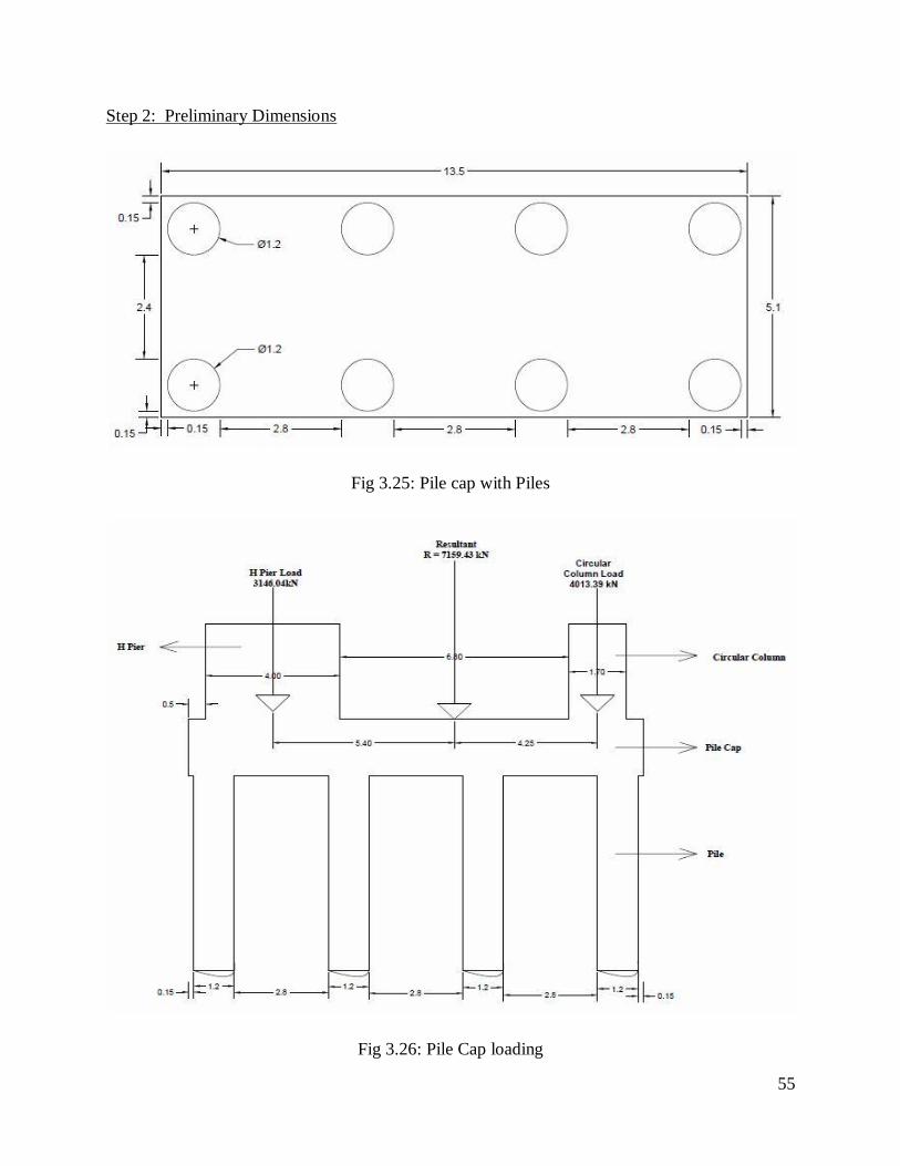
Step 2: Preliminary Dimensions

Fig 3.25: Pile cap with Piles

Fig 3.26: Pile Cap loading

56

Diameter of pile, d = 1200 mm

Here, a pile cap is designed for a group of eight piles of diameter 1200 mm.

As per IS 2911, Cl 6.6.1,

Spacing between 2 piles = 2d to 2.5d = 2400 mm to 3000mm

Breadth of pile cap = 2400 + (2 × 1200) + (2 × 150)

= 5100 mm

Depth of pile cap = Development length of column bar + Cover+ Projection

As per Table 65 of SP 16: 1980,

For 25 mm dia bars, development length, Ldt = 940 mm

Assuming a clear cover of 150 mm and a 50 mm projection of pile in to the cap concrete

Depth of pile cap = 940 + 50 + 150 + 150 = 1290 mm

Provide a depth of 1800 mm for the pile cap

Length of pile cap = (4 x 1200) + (3 x 2800) + (2 x 150) = 13500mm

Hence, size of pile cap = 13500 mm x 5100 mm x 1800 mm

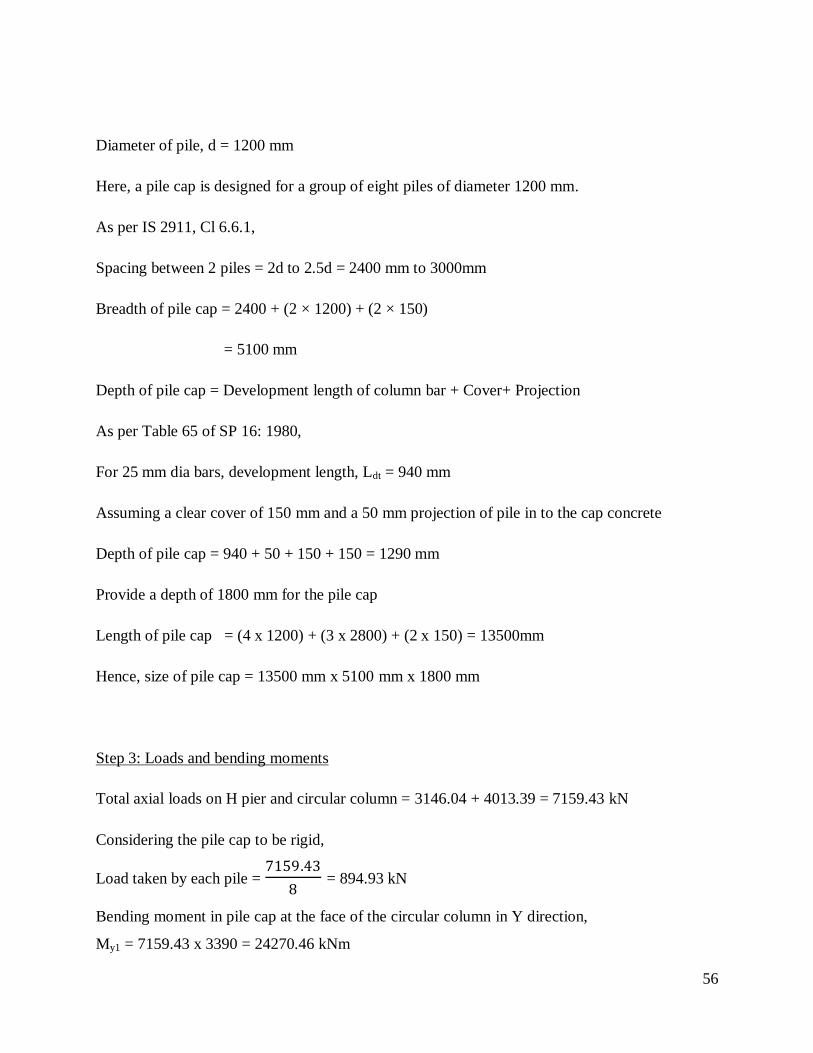
Step 3: Loads and bending moments

Total axial loads on H pier and circular column = 3146.04 + 4013.39 = 7159.43 kN

Considering the pile cap to be rigid,

Load taken by each pile = 7159.43

8 = 894.93 kN

Bending moment in pile cap at the face of the circular column in Y direction,

My1 = 7159.43 x 3390 = 24270.46 kNm

57

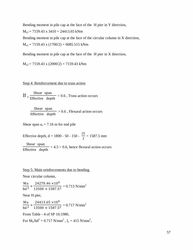
Bending moment in pile cap at the face of the H pier in Y direction,

My2 = 7159.43 x 3410 = 24413.65 kNm

Bending moment in pile cap at the face of the circular column in X direction,

Mx1 = 7159.43 x (1700/2) = 6085.515 kNm

Bending moment in pile cap at the face of the H pier in X direction,

Mx2 = 7159.43 x (2000/2) = 7159.43 kNm

Step 4: Reinforcement due to truss action

If , Shear span

Effective depth < 0.6 , Truss action occurs

Shear span

Effective depth > 0.6 , Flexural action occurs

Shear span av = 7.16 m for end pile

Effective depth, d = 1800 - 50 - 150 - 25

2 = 1587.5 mm

Shear span

Effective depth = 4.5 > 0.6, hence flexural action occurs

Step 5: Main reinforcements due to bending

Near circular column,

Mu

bd 2 = 24270 .46 ×106

13500 × 1587.52 = 0.713 N/mm2

Near H pier,

Mu

bd 2 = 24413 .65 ×106

13500 × 1587.52 = 0.717 N/mm2

From Table - 4 of SP 16:1980,

For Mu/bd2 = 0.717 N/mm

2 , fy = 415 N/mm

2,

58

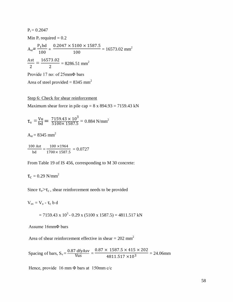
Pt = 0.2047

Min Pt required = 0.2

Ast= Pt bd

100 =

0.2047 × 5100 × 1587.5

100 = 16573.02 mm

2

Ast

2 =

16573.02

2 = 8286.51 mm

2

Provide 17 no: of 25mmΦ bars

Area of steel provided = 8345 mm2

Step 6: Check for shear reinforcement

Maximum shear force in pile cap = 8 x 894.93 = 7159.43 kN

τv = Vubd = 7159.43 × 103

5100× 1587.5 = 0.884 N/mm2

Ast = 8345 mm2

100 Ast

bd =

100 ×1964

1700 × 1587.5 = 0.0727

From Table 19 of IS 456, corresponding to M 30 concrete:

τc = 0.29 N/mm2

Since τv>τc , shear reinforcement needs to be provided

Vus = Vu - τc b d

= 7159.43 x 103 - 0.29 x (5100 x 1587.5) = 4811.517 kN

Assume 16mmΦ bars

Area of shear reinforcement effective in shear = 202 mm2

Spacing of bars, Sv = 0.87 dfyAsv

Vus = 0.87 × 1587.5 × 415 × 202

4811.517 ×103 = 24.06mm

Hence, provide 16 mm Φ bars at 150mm c/c

59

Fig 3.27 : Reinforcement Details of Pile Cap

5.1.12. APRON AND CUTOFF

The third stage of regulator will have 17 spans of 13.22m centre to centre distance.The critical

differential heads under which the regulator has to be operated is as follows:

Step 1: Water head

When the shutters are down,

Water on paddy fields side = 1.22m

Water on sea side = -0.46m

Maximum differential head = 1.22+0.46 = 1.68m

In the reverse direction (shutters are open),

Water on sea side = 0.85m

Water on land side = - 0.61m

Max differential head = 0.85 - 0.61 = 0.24m

60

So design the foundation apron for a critical differential head of 1.8m on either direction.

Step 2: Discharge based on maximum flood level

Maximum probable monsoon flood is calculated as follows:

Ryve‘s formula, Q = CA (2/3)

=8.45 x1124(2/3)

=913.5 cumec

Q = Discharge in cumecs

C = Flood coefficient (obtained from Table 1)

Table 3.10: Flood coefficient in Ryve‘s formula

Location of catchment C

1. Areas within 24km from coast 6.75

2. Areas within 24km to 161km from Coast 8.45

3. Limited areas near hills 10.1

Discharge through Thottapilly spillway = 400cumec (From records)

Net discharge Q‘ = Total discharge – Discharge through spillway

= 913.5- 400

= 513.5 cumec

Length of waterway L = Number of spans x span = 17 x 13.22 = 224.74m

Discharge per unit width, q = Q ′

L =

513.5

224.74 = 2.28 cumec/m

Scour depth R = [1.35( q2

f)(1/3)

]x 1.9

= [1.35( 2.282

1)

(1/3)]x 1.9

=4.44 m

61

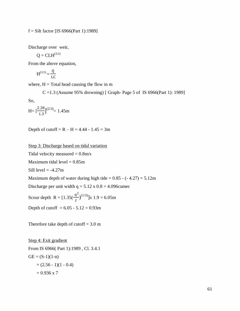
f = Silt factor [IS 6966(Part 1):1989]

Discharge over weir,

Q = CLH(3/2)

From the above equation,

H(3/2)

= Q

LC

where, H = Total head causing the flow in m

C =1.3 (Assume 95% drowning) [ Graph- Page 5 of IS 6966(Part 1): 1989]

So,

H= [2.28

1.3](2/3)

= 1.45m

Depth of cutoff = R – H = 4.44 - 1.45 = 3m

Step 3: Discharge based on tidal variation

Tidal velocity measured = 0.8m/s

Maximum tidal level = 0.85m

Sill level = -4.27m

Maximum depth of water during high tide = 0.85 - (- 4.27) = 5.12m

Discharge per unit width q = 5.12 x 0.8 = 4.096cumec

Scour depth R = [1.35( q2

f)

(1/3)]x 1.9 = 6.05m

Depth of cutoff = 6.05 - 5.12 = 0.93m

Therefore take depth of cutoff = 3.0 m

Step 4: Exit gradient

From IS 6966( Part 1):1989 , Cl. 3.4.1

GE = (S-1)(1-n)

= (2.56 - 1)(1 - 0.4)

= 0.936 x 7

62

= 6.55

where,

S = Specific gravity

n = Porosity

Safe exit gradient = 1

GE =

1

6.55 ≈

1

7

Step 5: Dimensions of apron

We have ,

GE = H

d x

1

π √λ

1

7 =

1.8

2.7 x

1

π √λ

i.e, 1

π √λ = 0.21

which implies α = 4.0

From Khosla‘s curve

α = b

d = 4.0

b = 4.0 x 2.7 ≈ 11 m.

i.e, Length of apron = 11 m.

From Khosla‘s curve,

1

α = 0.2

ΦD = 28

ΦE=40

ΦC1 = 100 - ΦE = 100- 40 = 60%

ΦD1 = 100 - ΦD = 100- 28 = 72%

a) Correction for mutual interference

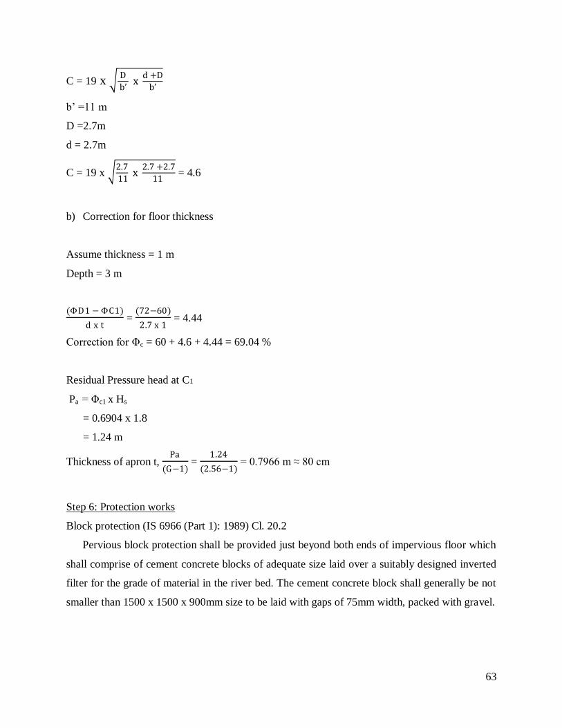
63

C = 19 x D

b’ x

d +D

b’

b‘ =11 m

D =2.7m

d = 2.7m

C = 19 x 2.7

11 x

2.7 +2.7

11 = 4.6

b) Correction for floor thickness

Assume thickness = 1 m

Depth = 3 m

(ΦD1 − ΦC1)

d x t =

(72−60)

2.7 x 1 = 4.44

Correction for Φc = 60 + 4.6 + 4.44 = 69.04 %

Residual Pressure head at C1

Pa = Φc1 x Hs

= 0.6904 x 1.8

= 1.24 m

Thickness of apron t, Pa

(G−1) =

1.24

(2.56−1) = 0.7966 m ≈ 80 cm

Step 6: Protection works

Block protection (IS 6966 (Part 1): 1989) Cl. 20.2

Pervious block protection shall be provided just beyond both ends of impervious floor which

shall comprise of cement concrete blocks of adequate size laid over a suitably designed inverted

filter for the grade of material in the river bed. The cement concrete block shall generally be not

smaller than 1500 x 1500 x 900mm size to be laid with gaps of 75mm width, packed with gravel.

64

The length of block protection shall be approximately equal to 1.5D where this length is

substantial, block protection with inverted filter may be provided in part of the length and block

protection only with loose stone spawls in remaining length.

Fig 3.28: Apron And Cutoff Wall

65

CHAPTER 4

CONCLUSIONS

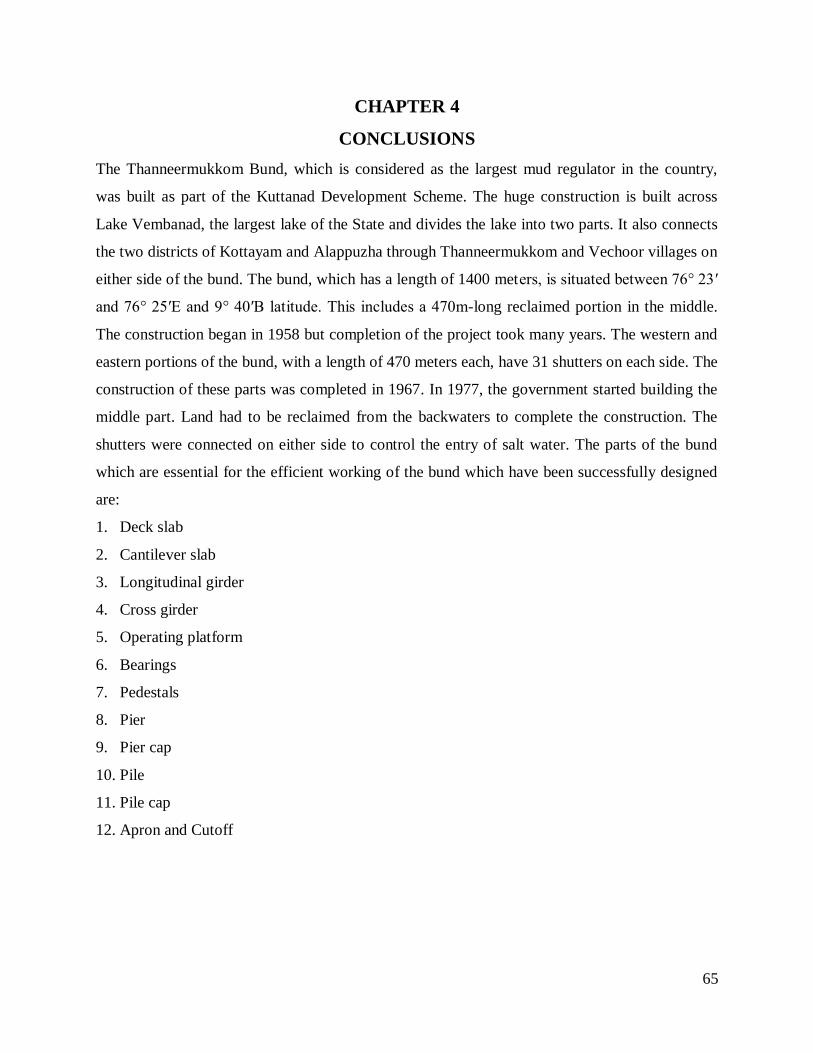
The Thanneermukkom Bund, which is considered as the largest mud regulator in the country,

was built as part of the Kuttanad Development Scheme. The huge construction is built across

Lake Vembanad, the largest lake of the State and divides the lake into two parts. It also connects

the two districts of Kottayam and Alappuzha through Thanneermukkom and Vechoor villages on

either side of the bund. The bund, which has a length of 1400 meters, is situated between 76° 23′

and 76° 25′E and 9° 40′B latitude. This includes a 470m-long reclaimed portion in the middle.

The construction began in 1958 but completion of the project took many years. The western and

eastern portions of the bund, with a length of 470 meters each, have 31 shutters on each side. The

construction of these parts was completed in 1967. In 1977, the government started building the

middle part. Land had to be reclaimed from the backwaters to complete the construction. The

shutters were connected on either side to control the entry of salt water. The parts of the bund

which are essential for the efficient working of the bund which have been successfully designed

are:

1. Deck slab

2. Cantilever slab

3. Longitudinal girder

4. Cross girder

5. Operating platform

6. Bearings

7. Pedestals

8. Pier

9. Pier cap

10. Pile

11. Pile cap

12. Apron and Cutoff

66

CHAPTER 5

SCOPE FOR FUTURE WORK

Analysis and designs of different components are done based on general procedures and software

available. But various limitations, as listed below, are present which could be overcome in

future, if proper facilities become available.

1. Pier analysis in STAAD.Pro encountered limitations in considering sloshing effect and

earthquake effect.

2. As the time for completion of project work is limited, only a single span is considered for

analysis and design based on the single span is provided for the whole structure.

67

REFERENCES

1. Amit Saxena, Dr.Savita Maru. (2013), ―Comparative Study of the Analysis and Design of T-

Beam Girder and Box Girder Superstructure‖, IJREAT, International Journal of Research in

Engineering & Advanced Technology

2. Arnold W. Hendry , Leslie G. Jaeger. (1955), “The Load Distribution in Interconnected

Bridge Girders with Special Reference to Continuous Beams”, Publisher- IABSE

publications, Memoires AIPC,IVBH Abhandlungen

3. H P Santhosh, Dr. H M Rajashekhara Swamy, Dr. D L Prabhakara. (2014), ―Construction Of

Cofferdam -A Case Study‖, IOSR Journal of Mechanical and Civil Engineering (IOSR-

JMCE)

4. IS 2911-1-1 (2010): Design and Construction of Pile Foundations — Code of Practice, Part

1: Concrete Piles

5. IS 456: 2000, Plain and Reinforced concrete

6. Kavitha.N, Jaya kumari.R, Jeeva.K, Bavithra.K, Kokila.K. (2015), ―Analysis and Design of

Flyover‖, National Conference on Research Advances in Communication, Computation,

Electrical Science and Structures (NCRACCESS-2015)

7. Manjeetkumar M Nagarmunnoli and S V Itti. (2014), ―Effect of Deck Thickness in RCC T-

beam Bridge‖, International Journal of Structural and Civil Engineering Research, ISSN

2319 – 6009, Vol. 3, No. 1

8. M.G. Kalyanshetti, C.V. Alkunte. (2012), ―Study on Effectiveness of IRC Live load on

R.C.R Bridge Pier‖, International Journal of Advanced Technology in Civil Engineering,

ISSN: 2231 –5721, Volume-1, Issue-3,4

9. Mundzir Hasan Basri. (2001), ―Two New Methods for Optimal Design of Subsurface

Barrier to Control Seawater Intrusion‖

10. Nan Hu, Gonglian Dai. (2010), ―The Comparative Study of Portal-Frame Pier for High-

Speed Railway‖

11. N. Krishna Raju. (2013), “Advanced Reinforced Concrete Design (IS:456-2000)”, Publisher-

CBS Publisher, Edition-2

68

12. Parvin Eghbali, Amir Ahmad Dehghani, Hadi Arvanaghi, Maryam Menazadeh. (2013), ―The

Effect of Geometric Parameters and Foundation Depth on Scour Pattern around Bridge Pier‖,

Journal of Civil Engineering and Urbanism, Volume 3, Issue 4: 156-163

13. P.N.Modi. (2008), “Irrigation Water Resources and Water Power Engineering”, Publisher-

Standard Book House Delhi, Edition-7

14. Praful N K , Balaso Hanumant. (2015), ―Comparative Analysis of T-Beam Bridge by

Rational Method and Staad Pro‖, International Journal of Engineering Sciences & Research

Technology

15. SP 16 : 1980

16. S. Ponnuswamy (2007), “Bridge Engineering”, Publisher- Mcgraw Hill Education, Edition-2

17. ―Study for modernizing the Thanneermukkom bund and Thottappally spillway for efficient

water management in Kuttanad region, Kerala‖, Indian Institute of Technology,

Madras,Chennai and Centre for Water Resources Development and Management,

Kozhikode, Kerala (2011)

18. Victor, Johnson D. (2007), “Essentials of Bridge Engineering”, Publisher- Oxibh, Edition-6

69

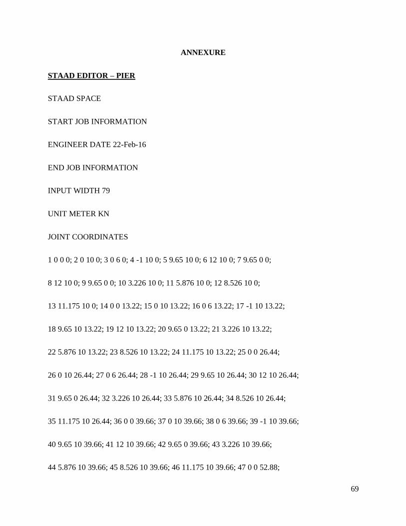
ANNEXURE

STAAD EDITOR – PIER

STAAD SPACE

START JOB INFORMATION

ENGINEER DATE 22-Feb-16

END JOB INFORMATION

INPUT WIDTH 79

UNIT METER KN

JOINT COORDINATES

1 0 0 0; 2 0 10 0; 3 0 6 0; 4 -1 10 0; 5 9.65 10 0; 6 12 10 0; 7 9.65 0 0;

8 12 10 0; 9 9.65 0 0; 10 3.226 10 0; 11 5.876 10 0; 12 8.526 10 0;

13 11.175 10 0; 14 0 0 13.22; 15 0 10 13.22; 16 0 6 13.22; 17 -1 10 13.22;

18 9.65 10 13.22; 19 12 10 13.22; 20 9.65 0 13.22; 21 3.226 10 13.22;

22 5.876 10 13.22; 23 8.526 10 13.22; 24 11.175 10 13.22; 25 0 0 26.44;

26 0 10 26.44; 27 0 6 26.44; 28 -1 10 26.44; 29 9.65 10 26.44; 30 12 10 26.44;

31 9.65 0 26.44; 32 3.226 10 26.44; 33 5.876 10 26.44; 34 8.526 10 26.44;

35 11.175 10 26.44; 36 0 0 39.66; 37 0 10 39.66; 38 0 6 39.66; 39 -1 10 39.66;

40 9.65 10 39.66; 41 12 10 39.66; 42 9.65 0 39.66; 43 3.226 10 39.66;

44 5.876 10 39.66; 45 8.526 10 39.66; 46 11.175 10 39.66; 47 0 0 52.88;

70

48 0 10 52.88; 49 0 6 52.88; 50 -1 10 52.88; 51 9.65 10 52.88; 52 12 10 52.88;

53 9.65 0 52.88; 54 3.226 10 52.88; 55 5.876 10 52.88; 56 8.526 10 52.88;

57 11.175 10 52.88;

MEMBER INCIDENCES

1 1 3; 2 3 2; 3 2 4; 4 2 10; 5 10 11; 6 11 12; 7 12 5; 8 5 13; 9 13 6; 10 5 7;

11 14 16; 12 16 15; 13 15 17; 14 15 21; 15 21 22; 16 22 23; 17 23 18; 18 18 24;

19 24 19; 20 18 20; 21 25 27; 22 27 26; 23 26 28; 24 26 32; 25 32 33; 26 33 34;

27 34 29; 28 29 35; 29 35 30; 30 29 31; 31 36 38; 32 38 37; 33 37 39; 34 37 43;

35 43 44; 36 44 45; 37 45 40; 38 40 46; 39 46 41; 40 40 42; 41 47 49; 42 49 48;

43 48 50; 44 48 54; 45 54 55; 46 55 56; 47 56 51; 48 51 57; 49 57 52; 50 51 53;

51 10 21; 52 21 32; 53 32 43; 54 43 54; 55 11 22; 56 22 33; 57 33 44; 58 44 55;

59 12 23; 60 23 34; 61 34 45; 62 45 56; 63 13 24; 64 24 35; 65 35 46; 66 46 57;

DEFINE MATERIAL START

ISOTROPIC CONCRETE

E 2.17185e+007

POISSON 0.17

DENSITY 23.5616

ALPHA 1e-005

DAMP 0.05

71

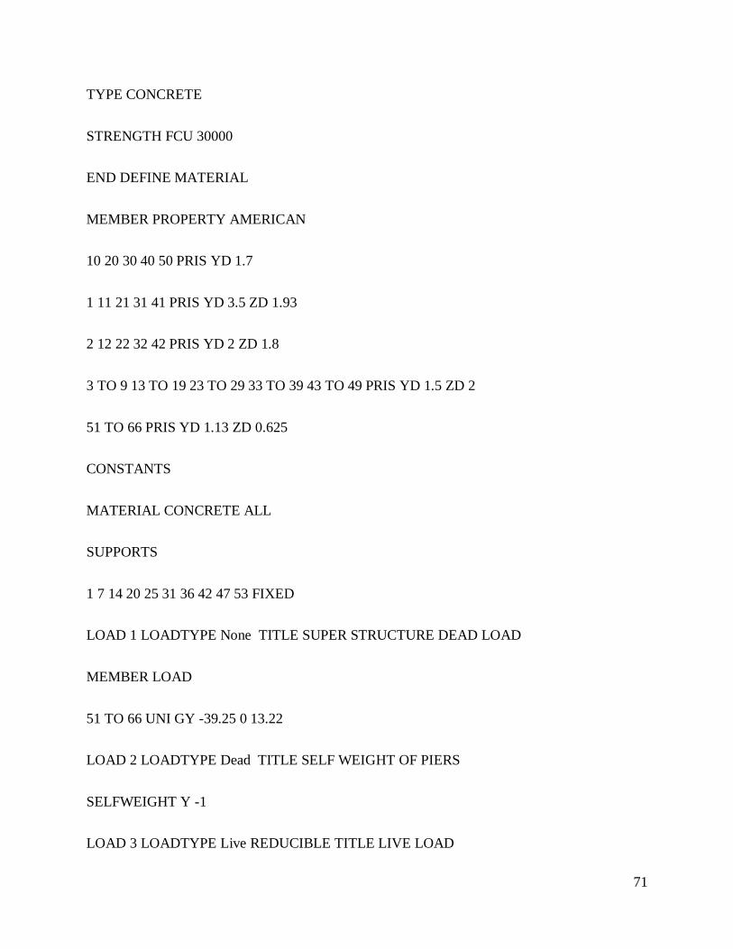
TYPE CONCRETE

STRENGTH FCU 30000

END DEFINE MATERIAL

MEMBER PROPERTY AMERICAN

10 20 30 40 50 PRIS YD 1.7

1 11 21 31 41 PRIS YD 3.5 ZD 1.93

2 12 22 32 42 PRIS YD 2 ZD 1.8

3 TO 9 13 TO 19 23 TO 29 33 TO 39 43 TO 49 PRIS YD 1.5 ZD 2

51 TO 66 PRIS YD 1.13 ZD 0.625

CONSTANTS

MATERIAL CONCRETE ALL

SUPPORTS

1 7 14 20 25 31 36 42 47 53 FIXED

LOAD 1 LOADTYPE None TITLE SUPER STRUCTURE DEAD LOAD

MEMBER LOAD

51 TO 66 UNI GY -39.25 0 13.22

LOAD 2 LOADTYPE Dead TITLE SELF WEIGHT OF PIERS

SELFWEIGHT Y -1

LOAD 3 LOADTYPE Live REDUCIBLE TITLE LIVE LOAD

72

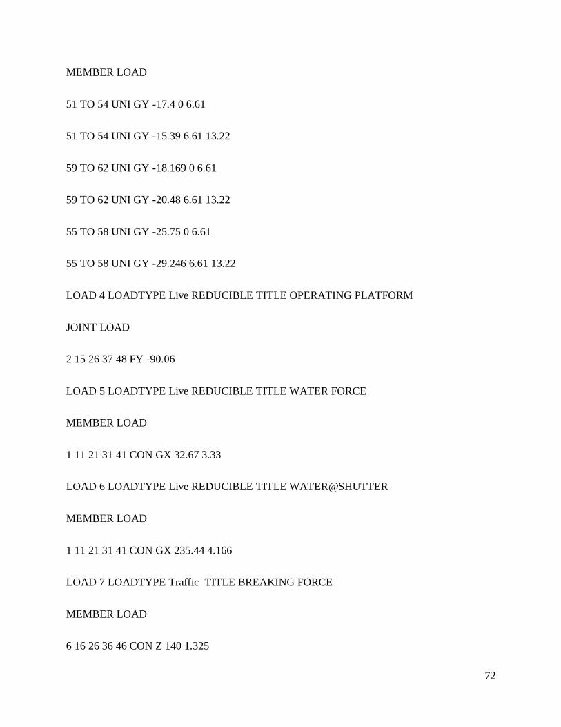
MEMBER LOAD

51 TO 54 UNI GY -17.4 0 6.61

51 TO 54 UNI GY -15.39 6.61 13.22

59 TO 62 UNI GY -18.169 0 6.61

59 TO 62 UNI GY -20.48 6.61 13.22

55 TO 58 UNI GY -25.75 0 6.61

55 TO 58 UNI GY -29.246 6.61 13.22

LOAD 4 LOADTYPE Live REDUCIBLE TITLE OPERATING PLATFORM

JOINT LOAD

2 15 26 37 48 FY -90.06

LOAD 5 LOADTYPE Live REDUCIBLE TITLE WATER FORCE

MEMBER LOAD

1 11 21 31 41 CON GX 32.67 3.33

LOAD 6 LOADTYPE Live REDUCIBLE TITLE WATER@SHUTTER

MEMBER LOAD

1 11 21 31 41 CON GX 235.44 4.166

LOAD 7 LOADTYPE Traffic TITLE BREAKING FORCE

MEMBER LOAD

6 16 26 36 46 CON Z 140 1.325

73

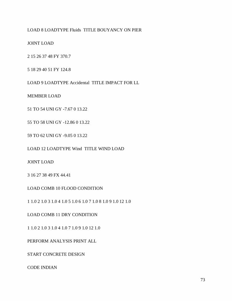
LOAD 8 LOADTYPE Fluids TITLE BOUYANCY ON PIER

JOINT LOAD

2 15 26 37 48 FY 370.7

5 18 29 40 51 FY 124.8

LOAD 9 LOADTYPE Accidental TITLE IMPACT FOR LL

MEMBER LOAD

51 TO 54 UNI GY -7.67 0 13.22

55 TO 58 UNI GY -12.86 0 13.22

59 TO 62 UNI GY -9.05 0 13.22

LOAD 12 LOADTYPE Wind TITLE WIND LOAD

JOINT LOAD

3 16 27 38 49 FX 44.41

LOAD COMB 10 FLOOD CONDITION

1 1.0 2 1.0 3 1.0 4 1.0 5 1.0 6 1.0 7 1.0 8 1.0 9 1.0 12 1.0

LOAD COMB 11 DRY CONDITION

1 1.0 2 1.0 3 1.0 4 1.0 7 1.0 9 1.0 12 1.0

PERFORM ANALYSIS PRINT ALL

START CONCRETE DESIGN

CODE INDIAN

74

CONCRETE TAKE

FC 30000 ALL

FYMAIN 415000 ALL

FYSEC 415000 ALL

DESIGN COLUMN 21 22 30

END CONCRETE DESIGN


FINISH

STAAD EDITOR – PIER CAP

STAAD SPACE

START JOB INFORMATION

ENGINEER DATE 22-Feb-16

END JOB INFORMATION

INPUT WIDTH 79

UNIT METER KN

JOINT COORDINATES

25 0 0 26.44; 26 0 10 26.44; 27 0 6 26.44; 28 -1 10 26.44; 29 9.65 10 26.44;

31 9.65 0 26.44; 32 12 10 26.44;

75

MEMBER INCIDENCES

21 25 27; 22 27 26; 30 29 31; 31 28 26; 32 26 29; 33 29 32;

DEFINE MATERIAL START

ISOTROPIC CONCRETE

E 2.17185e+007

POISSON 0.17

DENSITY 23.5616

ALPHA 1e-005

DAMP 0.05

TYPE CONCRETE

STRENGTH FCU 30000

END DEFINE MATERIAL

MEMBER PROPERTY AMERICAN

30 PRIS YD 1.7

21 PRIS YD 3.5 ZD 1.93

22 PRIS YD 2 ZD 1.8

31 TO 33 PRIS YD 1.5 ZD 2

CONSTANTS

MATERIAL CONCRETE ALL

76

SUPPORTS

25 31 FIXED

LOAD 1 LOADTYPE None TITLE SUPER STRUCTURE DEAD LOAD

MEMBER LOAD

32 CON Y -626.44 3.226

32 CON Y -626.44 5.876

32 CON Y -626.44 8.526

33 CON Y -626.44 0.825

LOAD 3 LOADTYPE Live REDUCIBLE TITLE LIVE LOAD

MEMBER LOAD

32 CON Y -216.74 3.226

32 CON Y -363.52 5.876

32 CON Y -255.64 8.526

LOAD 4 LOADTYPE Live REDUCIBLE TITLE OPERATING PLATFORM

JOINT LOAD

26 FY -90.06

LOAD 2 LOADTYPE None TITLE PIERCAP SELF WEIGHT

SELFWEIGHT Y -1 LIST 31 TO 33

LOAD COMB 5 COMBINATION LOAD CASE 5

77

1 1.0 3 1.0 4 1.0 2 1.0


START CONCRETE DESIGN

CODE INDIAN

FYSEC 415000 MEMB 21 22 30

CONCRETE TAKE

FYMAIN 415000 ALL

FYSEC 415000 ALL

FC 30000 ALL

DESIGN BEAM 31 TO 33

END CONCRETE DESIGN


FINISH