project number: salvador antoniou crn: 21493 erik … · 2010-03-05 · degree of bachelor of...

Project Number: Salvador Antoniou CRN: 21493

Erik Khzouz CRN: 21291

Trading System Development

An Interactive Qualifying Project Report

submitted to the Faculty

of the

WORCESTER POLYTECHNIC INSTITUTE

in partial fulfillment of the requirements for the

Degree of Bachelor of Science

by

Salvador Antoniou

&

Erik Khzouz

Date: March 5, 2010

Associate Professor Michael J. Radzicki, Major Advisor

1. trading system

2. stock

3. development

This report represents the work of one or more WPI undergraduate students submitted to the faculty as evidence of

completion of a degree requirement. WPI routinely publishes these reports on its web site without editorial or peer review.

2

Acknowledgements

First off, we would like to thank Professor Radzicki of the WPI Social Sciences

Department for supervising our project as well as offering us his guidance throughout. He was of

great help in steering us in a progressive direction with such an open ended project and the

resources he shared with us were of great use. We would also like to thank some specific

members of the TradeStation community that aided us modeling and coding. We thank

Greg@TSSec of TradeStation Securities for his assistance in the modeling of the MAGNET

Simple Scanner, which played an integral role in the project. We also offer our gratitude to Mark

J. Krisburg (MarkSanDiego) of the TradeStation forum community who helped Erik in the code

for the Expectancy portion of our analysis.

3

Abstract

The purpose of this IQP is to create a trading system using the TradeStation platform

based around the MAGNET Simple Scanner and daily bars. The scanner tells a user which

stocks have the potential to breakout, however it does not tell a trader when to enter or exit a

market. Thus, the value added by this project is characterized by the determination of successful

entries and exits through the studies done. This report is formatted in such a way as to first

provide some initial background for the reader regarding some trade and market concepts, as

well as information on the TradeStation Platform. We then move on to discuss some of the major

developments of the project regarding the strategies we employed and tested. Summarized

results in the forms of tables are included in these sections along with the conclusions drawn

from them. Next, some specific analysis techniques will be discussed when they were applied to

our leading strategy. Lastly, there is a miscellaneous works section that catalogs many of our

side developments along the way that did not see fruition, but whose outcomes were nonetheless

important to the progress of the project.

4

Table of Contents

I. Introduction ......................................................................................................................................... 9

1.1- Introduction Statement ............................................................................................................... 9

1.2 - Significance ................................................................................................................................. 9

1.3 - What the Project Entails ............................................................................................................. 9

1.4 - Project Goals ............................................................................................................................ 10

II. Background ....................................................................................................................................... 11

2.1 - What Is a Trade System ............................................................................................................ 11

2.2 - Parts of a Trade System ............................................................................................................ 11

Target Markets ............................................................................................................................. 11

Scanners ....................................................................................................................................... 12

Indicators ...................................................................................................................................... 13

Entry/Exit Conditions and Triggers ............................................................................................... 13

2.3 - TradeStation Platform .............................................................................................................. 14

2.4 - Resources ................................................................................................................................. 16

III. Scanner ............................................................................................................................................ 18

3.1 - Significance of Scanner ............................................................................................................. 18

3.2 - Types of Scanners Looked At .................................................................................................... 18

Types of Scanners ......................................................................................................................... 18

Main Scanners Focused On .......................................................................................................... 19

3.3 – Selection: The Magnet Simple Scanner ................................................................................... 20

Scanner Details ............................................................................................................................. 20

3.4 - Scanner Results and Final List of Stocks ................................................................................... 22

IV. Indicators ......................................................................................................................................... 23

4.1 - The ShowMe ............................................................................................................................. 23

4.2 - The Paintbar ............................................................................................................................. 24

4.3 - Conclusions ............................................................................................................................... 25

V. The First Strategy ............................................................................................................................. 26

5.1 - Strategy Basis ........................................................................................................................... 26

5.2 – Easy Language Code ................................................................................................................ 26

5.3 - Tests ......................................................................................................................................... 27

5.4 - Results ...................................................................................................................................... 29

Performance Summary ................................................................................................................. 30

Equity Curve ................................................................................................................................. 32

5

Trade Efficiency Graph ................................................................................................................. 33

Periodical Returns Table ............................................................................................................... 34

First Strategy Summary Tables ..................................................................................................... 35

VI. The Volume Entry Strategy ............................................................................................................. 37

6.1 - Strategy Basis ........................................................................................................................... 37

6.2 – Easy Language Code ................................................................................................................ 37

6.3 - Tests ......................................................................................................................................... 38

6.4 - Results ...................................................................................................................................... 38

Volume Entry Summary Tables .................................................................................................... 39

VII. The Volume Exit Strategy ............................................................................................................... 40

7.1 - Strategy Basis ........................................................................................................................... 40

7.2 - Easy Language Code ................................................................................................................. 40

7.3 - Tests ......................................................................................................................................... 41

7.4 - Results ...................................................................................................................................... 42

Volume Exit Summary Tables ....................................................................................................... 43

VIII. The LeBeau Exit Strategy ............................................................................................................... 45

8.1 - Strategy Basis ........................................................................................................................... 45


8.3 - Tests ......................................................................................................................................... 47

8.4 – Results ..................................................................................................................................... 48

LeBeau Exit Summary Tables ........................................................................................................ 49

IX. The LeBeau Short Exit Strategy ....................................................................................................... 51

9.1 - Strategy Basis ........................................................................................................................... 51


9.3 - Tests ......................................................................................................................................... 52

9.4 - Results ...................................................................................................................................... 53

LeBeau Exit Summary Tables ........................................................................................................ 53

X. Analysis Techniques – Expectancy and Expectunity ......................................................................... 55

10.1 - Expectancy .............................................................................................................................. 55

EasyLanguage Code ...................................................................................................................... 56

Results .......................................................................................................................................... 57

10.2 - Expectunity ............................................................................................................................. 57

Formulation .................................................................................................................................. 57

Results .......................................................................................................................................... 58

XI. Miscellaneous Strategies and Other Works .................................................................................... 59

6

11.1 - The Charlie Wright Coke Strategy .......................................................................................... 59

11.2 - Exit with a Profit/Exit with a Loss ........................................................................................... 60

11.3 - Exchange-Traded Fund (ETF) .................................................................................................. 61

11.4 - The Chicago Board Options Exchange Volatility Index (VIX) .................................................. 62

XII. Concluding the Development ......................................................................................................... 64

12.1 - Final Optimization .................................................................................................................. 64

12.2 - Results .................................................................................................................................... 64

12.3 - Real Time Simulation .............................................................................................................. 65

12.4 - Going Further ......................................................................................................................... 66

Position Sizing ............................................................................................................................... 66

Monte Carlo Analysis .................................................................................................................... 66

XIII. Closing Statement ......................................................................................................................... 67

Appendix ............................................................................................................................................... 68

Section A: TradeStation Easy Language Code .................................................................................. 68

Section B: First Strategy (2004-2008) ............................................................................................... 88

Sample of Strategy Overlay on Stock Chart .................................................................................. 88

Performance Summaries .............................................................................................................. 91

Equity Curves ................................................................................................................................ 99

Trade Efficiency Graphs .............................................................................................................. 103

Periodic Returns ......................................................................................................................... 107

Section C: Volume Entry (2004-2008) ............................................................................................ 111

Sample of Strategy Overlay on Stock Chart ................................................................................ 111

Performance Summaries ............................................................................................................ 114

Equity Curves .............................................................................................................................. 122


Periodic Returns ......................................................................................................................... 130

Section D: Volume Entry (2004-2008) ............................................................................................ 134



Equity Curves .............................................................................................................................. 145


Periodical Returns ...................................................................................................................... 153

Section E: Volume Entry (2007-2009) ............................................................................................ 157



7

Equity Curves .............................................................................................................................. 168



Section F: Volume Entry 2004-2009 ............................................................................................... 180



Equity Curves .............................................................................................................................. 191



Section G: LeBeau Exit 2004-2008 .................................................................................................. 203



Equity Curves .............................................................................................................................. 214



Section H: LeBeau Exit (2007-2009) ............................................................................................... 226



Equity Curves .............................................................................................................................. 237



Section I: LeBeau Exit Short (2004-2008) ....................................................................................... 248



Equity Curves .............................................................................................................................. 259



Section J: LeBeau Exit Short (2007-2009) ....................................................................................... 271



Equity Curves .............................................................................................................................. 282



Section K: Communications with MarkSanDiego ........................................................................... 294

Bibliography ........................................................................................................................................ 298

8

Summary of Tables_____________________________

Table 1 - Value Scanners....................................................................................................................... 20 Table 2 - Growth Scanners ................................................................................................................... 20 Table 3 - Growth and Value Scanners .................................................................................................. 20 Table 4 - List of Stocks from Scanner.................................................................................................... 22 Table 5 - Summary of First Strategy Test Parameters .......................................................................... 28 Table 6 - First Strategy Optimized Variables ........................................................................................ 35 Table 7 - First Strategy Results Summary ............................................................................................. 36 Table 8 - Volume Entry Parameter Test Summary ............................................................................... 38 Table 9 - Volume Entry Strategy Optimized Variables ......................................................................... 39 Table 10 - Volume Entry Strategy Results Summary ............................................................................ 39 Table 11 - Volume Exit Strategy Parameter In-Sample-Test Summary ................................................ 41 Table 12 - Volume Exit Strategy Parameter Out-of-Sample Test Summary ......................................... 42 Table 13 - Volume Exit Strategy Optimized Variables .......................................................................... 43 Table 14 - Volume Exit Strategy Results Summary (2004-2008) .......................................................... 43 Table 15 - Volume Exit Strategy Results Summary (2007-2009) .......................................................... 44 Table 16 - LeBeau Exit Strategy Parameter In-Sample-Test Summary ................................................. 47 Table 17 - LeBeau Exit Strategy Parameter Out-of-Sample Test Summary ......................................... 48 Table 18 - LeBeau Exit Strategy Optimized Variables ........................................................................... 49 Table 19 - LeBeau Exit Strategy Results Summary (2004-2008) ........................................................... 49 Table 20 - LeBeau Exit Strategy Results Summary (2007-2009) ........................................................... 50 Table 21 - LeBeau Short Exit Strategy Parameter In-Sample-Test Summary ....................................... 52 Table 22 - LeBeau Short Exit Strategy Parameter Out-of-Sample Test Summary ................................ 52 Table 23 - LeBeau Short Exit Strategy Optimized Variables ................................................................. 53 Table 24 - LeBeau Short Exit Strategy Results Summary (2004-2008) ................................................. 54 Table 25 - LeBeau Short Exit Strategy Results Summary (2007-2009) ................................................. 54 Table 26 - Expectancy per Stock ........................................................................................................... 57 Table 27 - Expectunity per Stock .......................................................................................................... 58 Table 28 - Volume Exit Strategy Optimized Variables (2004-2009) ..................................................... 64 Table 29 - Volume Exit Strategy Results Summary (2004-2009) .......................................................... 65

9

I. Introduction

1.1- Introduction Statement

The ensuing IQP report documents the Trading System Development Project undertaken

by Salvador Antoniou and Erik Khzouz. The duration of the project spanned three consecutive

terms from the beginning of September 2009 to the end of February 2010. The project was

overseen by Professor M. J. Radzicki of the Social Sciences Department at WPI.

1.2 - Significance

Over the last decade, there has been a large emergence of trading platforms, such as

ScottTradeTM and AmeriTradeTM that allow an individual to take control of his or her financial

future. It has become very easy for the average citizen to access this technology through the

internet from the comfort of their own homes. The problem is that many of these users have no

real concept of what a trade system is. Frequently their decisions are based on recommendations

of other websites. They often do not dig deeper as to why the source is making the

recommendation that it does. The significance of this project is that it will demonstrate a method

by which the average individual can educate themselves about market trading through utilizing

the notion of a trading system. The value added by this project will be in constructing a

profitable trading system around a scanner, which is one of the components of such a system.

The scanner alone only tells the individual what stocks to buy, however does not tell them when

to buy in and when to exit.

1.3 - What the Project Entails

Throughout this document, the reader will get a glimpse of the journey made by two

engineering students delving into stock trading and system development. As engineering

students, we entered this project with only a rudimentary understanding of economics and do not

claim to have created a comprehensive, mother-of-all trade systems. Throughout the project, we

needed to do much research into terminology and trading functions (e.g. short-selling, buy-to-

10

cover, etc.) Many of these concepts and terms will be introduced and explained as we discover

them and integrate them into our project. The main portion of the project will be learning how to

use the TradeStation Platform and devising strategies that we think will be successful in

generating greater profits on investments. TradeStation allows us to simulate our theories on

historical stock data to see how it would have performed. From that we can determine a

system‟s viability. More on this will be discussed in the Background and Study sections further

into the report. Lastly, once we develop a strategy we feel is viable, we will further test our trade

system using some established analysis techniques that will be able to quantify its performance.

1.4 - Project Goals

In this part, we will outline the goals that we ascertained for this project upon its commencement.

- Gain insight into economics and stock trading

- Learn how use TradeStation and rule based trading

- Design and test a trading system scientifically

- Develop a profitable trading system

11

II. Background

In this part of the report we will be providing the reader with background concerning the

components of trading systems as well as some methodologies that go into the developmental

process. Furthermore, we will be addressing how we approached some of these aspects.

2.1 - What Is a Trade System

For our project, a trade system is defined as a computerized method that follows a set of

rules to trade in a given market. Hence, trade system development is the process by which one

determines the sets of rules and parameters for when to enter and exit a given market. It is a

methodical, scientific process involving a series of tests and analyses. Considering that we lack

the market insight that a seasoned economics major or investor has, our primary method of

analyses were trial and error and maximization. We tested some simple tactics that we

developed, as well as some more complex ones at the advice of our instructor and sought to

maximize the profit gained from our system. The procedure was found to be a modular process

in which we worked with interchangeable subsystems. Testing involved changing one

component and holding the rest constant so that outcomes could be compared.

2.2 - Parts of a Trade System

In our experience through the project, we have determined that a trade system can be

broken down into a handful of fundamental parts: the target markets, the scanner, indicators, and

entry/exit conditions and triggers.

Target Markets

The basis of a trade system lies in its target market. These markets include, but are not

limited to, equities, futures, FOREX, and bonds. Equities, traditionally known as stocks to those

outside of the profession, are the most commonly known market because of their ample coverage

12

by the media. Trading futures involves contracts to buy or sell commodities at certain dates in

the future. The FOREX is a foreign exchange market in which people take advantage of the

fluctuations in value between global currencies and trade them. Lastly, the bonds market is a

market where people buy and sell debt securities. For a seasoned investor, the target market is

important because it can carry a number of implications since each one has its own set of

tendencies.

For our project, we have chosen to center our system on trading equities because we have

some past experience with them. We also found them to be more straightforward than some of

the other market types and we wanted to pick a market we would be comfortable with as we

would be spending an ample amount of time with it.

Scanners

In a trade system, the scanner is akin to a stock filter and they make excellent tools for

finding stocks of a particular type one wishes to build a system around. Scanners take a set of

parameters, which can be based on any available company data and apply them to a market,

returning only the stocks that fulfill the conditions in the parameters. Such an example of a basic

parameter would be for the scanner to only return stocks of companies that have grown at least

10% YOY (Year over Year). This has powerful implications for trade system development

because it allows one to quickly isolate stocks of a particular type, allowing one to build a trade

system that is more likely to be consistent across the stocks it trades.

There are three main types of stock scanners, Growth Scans, Value Scan, Growth and

Value Scans. Growth screens look to identify potential stocks which are deemed to have a rapid

growth in earnings within the immediate future, while Value screens identify stocks that may be

trading at a discount to their intrinsic value. Lastly, there are Growth and Value Scans which, as

expected, is a hybrid type that combines certain aspects from both fields.

For the purposes of our project, we have opted to go with a Growth and Value scan

because it seemed like a balanced approach to us. More on the decision process is discussed in

the Scanner section of this report.

13

Indicators

The next type of tool in the trade system developer‟s arsenal to introduce is indicators.

Indicators are trade system tools that summarize data and are useful for highlighting emerging

trends within a chart. With easily visible trends, a system developer can make judgments and

modifications to their strategy with the bigger picture in mind. Because they highlight trends,

they tend to be simple in structure because more complex patterns can be more difficult to

analyze. An example of an indicator rule might be to paint bars on a price chart a specific color if

the bars of a stock are trending upward or downward.

Entry/Exit Conditions and Triggers

Entry/exit conditions are sets of rules in a trade system that tell the system when it should

buy and sell in a market. The triggers are the commands in the code that perform the buy and sell

function.

The rules for entries and exits are limited only by one‟s ingenuity and can be incredibly

simple or complex. There are many different ways to approach entry points. Examples include

entering as soon as the stock begins to trend upwards; to determining if a stock is underpriced; to

analyzing their liquidity and determining if the company is expected to experience growth in the

coming quarter. Exit points are similar in that they can be as simple as exiting as soon as a

specified profit has been made or as complex and comprehensive as the LeBeau exits that we

experimented with in our project. Complexity of a strategy though does not always mean it will

produce a greater yield as we discovered in our studies.

In some ways, entries and exits are related in that your entry point will often determine

your exit point. However, they can also be treated as independent of each other. In a short term

trading system you may wish to exit the market as soon as you have made a profit, however in a

long term trading system, one will be more inclined to ride out some of the lows or highs

because one‟s analysis has led them to believe that the stock will see even higher highs. It is

often said that knowing when to enter the market is the easier part; knowing when and how to

exit after making substantial gains or taking a loss is exceedingly more difficult.

Regarding triggers, it should be noted that while buying and selling sound like simple

functions, they are made much more dynamic by the fact that there are multiple ways to buy and

14

sell. An example of buying is the buy-to-cover function. Buy-to-cover involves closing out a

short position, which happens to be a type of selling function. A short position is betting that a

stock‟s price will go down. To make money off of this, one gets loaned the stock, sells it, and

buys it later from someone else to return it. Conversely, if the value of the stock increases, the

short position will cause the person to lose money. These examples are but two of many

techniques that modern trades have in their repertoire.

2.3 - TradeStation Platform

The main tool we used for this project was the TradeStation 8.6 Client program by

TradeStation Securities. It is an extensive tool to develop and test trading systems which give the

user great flexibility and freedom when designing a system. TradeStation accomplishes this

through EasyLanguage.

EasyLanguage is a coding language specific to TradeStation that allows a user to create

custom commands and strategies. EasyLanguage allows those without extensive computer

training to be able to create trading systems. The EasyLanguage Manual can be found on the

TradeStation website1.

TradeStation normally requires a monthly subscription fee of over $100 that can reach as

high as $500 depending on the types of features you wish to include. Luckily, through our

advisor, we have received developer accounts that will only cost us approximately $30 a month

where we will only be able to simulate our work. Figure 1 on the following page is an example

of the TradeStation interface.

1 https://www.tradestation.com/support/books/

15

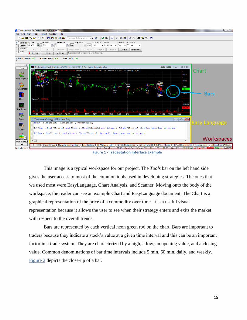
Figure 1 - TradeStation Interface Example

This image is a typical workspace for our project. The Tools bar on the left hand side

gives the user access to most of the common tools used in developing strategies. The ones that

we used most were EasyLanguage, Chart Analysis, and Scanner. Moving onto the body of the

workspace, the reader can see an example Chart and EasyLanguage document. The Chart is a

graphical representation of the price of a commodity over time. It is a useful visual

representation because it allows the user to see when their strategy enters and exits the market

with respect to the overall trends.

Bars are represented by each vertical neon green rod on the chart. Bars are important to

traders because they indicate a stock‟s value at a given time interval and this can be an important

factor in a trade system. They are characterized by a high, a low, an opening value, and a closing

value. Common denominations of bar time intervals include 5 min, 60 min, daily, and weekly.

Figure 2 depicts the close-up of a bar.

16

Figure 2 - Close-up Bar Representation

For our project, we have chosen to focus on daily bars. Due to our term schedule and how

fast the project would move, it was the best choice if we were to eventually progress to a point

where we ran our strategy in real time. Daily bars would allow us to pick up on fluctuations in

the stock price faster than weekly bars.

2.4 - Resources

Throughout our time working on this project we have had to turn to many different

sources to help us along. Our most comprehensive sources included Professor Radzicki, Charlie

Wright‟s book, Trading as a Business, the webpage for the American Association of

Independent Investors (AAII) and the TradeStation Forums. Each of these sources played a

pivotal role in shaping our trading system.

Professor Radzicki, throughout our project has helped to steer us in the right direction

offering both help and guidance as we worked toward our goal. Through our weekly meetings,

he scrutinized our results from the previous weeks as well as offered suggestions of what can be

done for the weeks ahead preventing us from losing sight of the bigger picture. He introduced us

to countless analysis techniques and tests that could be performed to evaluate our system‟s

performance, some of which are the LeBeau Exit and Expectancy/Expectunity. The LeBeau Exit

17

Strategy was developed by Charles “Chuck” LeBeau. His website can be found here2.

Expectancy and Expectunity are concepts that were developed by Van Tharp. An exposition on

this topic by Van Tharp can be referenced in an article published by The Trader’s Journal3.

Charlie Wright‟s book, Trading as a Business, was our first encounter with trading

systems development. Within his book, Wright lays the foundation for how one should proceed

to build a trading system. The emphasis throughout his book is to not build the “holy grail”

trading system, but to design one that can trade a particular market type. Wright also introduced

the possibility of trading with a stock screener to narrow down the pool of potential stocks to a

more manageable number. The full version of his book can be found online here4.

The homepage of the American Association of Independent Investors was suggested to us

by Professor Radzicki. This page became a pivotal cornerstone of our trading system once the

idea of using a stock screener became clear. AAII hosts a section of their site dedicated to over

50 different stock screeners which are updated on a monthly cycle. Each of these scans is placed

in one of three categories, Value Screens, Growth Screens as well as Growth and Value Screens.

The amount of information for each scan is extensive, including Screening Criteria, Performance

Charts, as well as Passing Companies. Scans can be compared to one another by comparing their

percent return on both year to date and total time frames. This webpage allowed us to see a broad

range of scanners and to narrow the list down to the top performing stocks within each category

and ultimately choose the MAGNET Scanner used in this project.

The TradeStation forum community5 is a thriving database of knowledge contributed by a

vast number of investors around the world. Countless times, we searched through the forums

when we were met with a roadblock in our design process. Whether it was assistance in

modeling the MAGNET Simple scanner, or it was attempting to get the Expectancy Function to

perform correctly, the TradeStation community was able to aid us in our process.

2 http://www.traderclub.com/

3 http://www.mtptrader.com/TJMay.pdf

4 http://www.elitetrader.com/tr/index.cfm

5 https://www.tradestation.com/Discussions/Forum.aspx?Forum_ID=213

18

III. Scanner

This section of the report catalogs the research, selection, and modeling of choosing a

stock scanner.

3.1 - Significance of Scanner

Throughout the length of our project, the stock scanner played a vital role in the success

of our strategy. A scanner allows the user to search through a vast database of information and to

filter out unwanted results, leaving a desired handful. For instance, in our project we used a stock

scanner which scans through all possible 7,876 stocks to return a total of eight. The scanner

became the cornerstone of our strategy, and thus would eventually lead to the success or failure

of our system.

3.2 - Types of Scanners Looked At

While researching different scanners, many different avenues were investigated with

eventual success or failure of each. Initial research of scanners led us to Google Finance™ which

houses their own stock scanner. Google‟s scan allows the user the ability to customize the

criteria filters that the scanner will use as well as specify exchange and sector to analyze. The

shortcomings of the Google Finance™ scanner are that the scans cannot be saved and thus would

have to be recreated each time a new scan was performed. Another issue that arose is that the

equities that passed the scan would have to manually be inserted into TradeStation of analysis.

Upon examination of TradeStation‟s toolbar, the program includes a built in Scanner tool

to aid traders. This native scanner allows for a greater level of customization and convenience

since actions such as Scheduling and Notification are integrated into the platform.

Types of Scanners

Once we had chosen to use TradeStation‟s native scanner, we were faced with either

creating our own screener or using one that had already been tested and has historical

performance data. Given that the scanner is the pivotal component that the rest of the strategy

19

would be based upon, the decision to use an already established scan was made. Professor

Radzicki in one of our meetings suggested we use the American Association for Independent

Investors (AAII) webpage as we focus on choosing the correct scanner. The AAII6 webpage has

a comprehensive list of over 50 different scans that are updated on a monthly basis. These scans

are separated into three main sections: Value, Growth, and Growth and Value.

Value scans seek to profit from misjudgments by other investors. This is done by

searching for “unfashionable stocks” which other investors have passed by for those that may

have been swept up in “market euphoria”. Once the euphoria has passed, investors rediscover the

once overlooked stocks. The idea is to locate these overlooked stocks before the spotlight shifts

upon them.

Growth scans seek to locate stocks that are about to jump. Companies that pass a growth

scan are generally growing above the rate of the overall economy (20% annual growth rate in

earnings per share). An important weakness to a growth stock is that the internal cash flow

occasionally cannot support the growth rate and thus more shares of the company are issued by

the corporation diluting the shares of current shareholders.

Growth and Value scans are an attempt to create a marriage between both Growth and

Value scans. This merger attempts to locate undervalued stocks that have high growth rates.

Since both Value and Growth scans attempt to locate niche stocks that have individually proven

to be successful, locating a stock which can bridge the gap between the two scans would allow

for the highest chance of success when investing.

Main Scanners Focused On

To narrow down the list of over 50 scans to a more manageable list, we decided to focus

on the top three performing scanners from each of the three categories. The performance of each

of these scans can be seen in the following three tables below.

% Return YTD % Return Total

Price to Free Cash Flow 108.6 605

Fundamental Rule of Thumb 68.1 649

6 http://www.aaii.com/

20

Dreman With Est Revisions 51.2 363.5 Table 1 - Value Scanners


O’Neil’s CANSLIM 88.9 2641.4

Driehaus 74.7 152.7

IBD Stable 70 36.9 144.2 Table 2 - Growth Scanners


MAGNET Simple 240.8 819.6

MAGNET Complex 20.7 813.8

Fisher (Philip) 90 140.2

Magic Formula 76.8 307.8 Table 3 - Growth and Value Scanners

In Table 3, there are four scanners listed instead of three. The reasoning for this is that

MAGNET Simple and MAGNET Complex are virtually built from the same foundation, but

have just been tweaked slightly to better suit the user.

3.3 – Selection: The Magnet Simple Scanner

Upon further review of our now smaller pool of scanners to choose from, we ultimately

chose the MAGNET Simple Scan. In the process of eliminating scanner types, we decided that

we wanted to go with a Growth and Value Scan because we wanted to work with stocks that

were growing steadily with the potential to have large moves. Another reason we settled on this

particular scanner was for its YTD and percent returns.

Scanner Details

The MAGNET Scan is an acronym, where each letter stands for a certain scanning

criteria. Management / Momentum (M), Acceleration in Revenues / Earnings (A), Growth at a

Reasonable Price (G), New Products / Management (N), Emerging Products / Industry (E),

Timing (T). Each letter provides a specific action to the overall scan, when viewed holistically a

sturdy framework is built to ensure that companies who pass through the scan are making a

valuable contribution to their respective industry. The MAGNET Scan itself is two scans in one,

MAGNET Simple and MAGNET Complex. The differences between these two scans are which

21

letters of MAGNET they encompass. MAGNET Simple uses M.A.G. while Complex uses

M.A.G.N.E.T. The Simple scan provides for a basic scan covering the basis which qualifies it as

a Growth and Value Screener, growing momentum, acceleration in earnings, and growth at a

reasonable price. The Complex scan provides for a more complete scan which encompasses all

aspects of the simple scan as well as product development, management and a minimum stock

price.

Ultimately we further narrowed our choice down to the MAGNET Simple over the

MAGNET Complex because the Complex version was too selective and we were not getting

enough results to work with. Below in Figure 3, an image of the Scan Criteria tab can be seen

which lists these criteria used. The amount of customization of each scan can be seen in the drop

down menu also in Figure 3.

22

Figure 3 - MAGNET Scanner Details

3.4 - Scanner Results and Final List of Stocks

The MAGNET Simple scan was modeled in TradeStation using criteria from the AAII

webpage which lists the filters that the scanner applies. The results of the MAGNET Simple scan

can be seen in Table 4.

Passing Stocks for MAGNET Simple Scan

APWR

CLMT

JST

KGS

NEU

NGLS

NRGP

NXG Table 4 - List of Stocks from Scanner

A scanner searches for stocks that currently pass its filters. Due to this restriction, it is not

possible to run the scanner on a specific date in the past to see if a particular stock would have

appeared. To deal with this, Professor Radzicki advised that we use the assumption that “stocks

that show up on a scan are “hot” stocks, and it can be assumed that they have always shown up

as results”. For this reason we decided to keep the eight original stocks shown in Table 4 for our

development and analysis later in the project. A discrepancy was observed between the results

we received from our scanner modeled in TradeStation and the expected results from AAII's scan

results web page. Multiple factors could attribute to the skewed data, the most prominent being

the accessibility of data. TradeStation uses real time data in its Scanner algorithm, allowing for

up to the minute, on demand results. In contrast, AAII's scans are updated in the middle of each

month with prior month-end data, allowing for accurate, but heavily delayed results.

23

IV. Indicators

While in the process of narrowing down a scanner, we simultaneously began working on

strategy formulation. As stated earlier, indicators are tools used to highlight emerging patterns in

charts of stock data. Using an indicator would allow us to take a structured approach and

provide us with a concrete reference point for further work.

4.1 - The ShowMe

The first study that we worked on was called a ShowMe. The ShowMe paints a colored

dot on a bar that meets a condition. Span this over multiple bars and it becomes easier to tell

whether a stock is trending upwards or downwards and how much time it spends in such phases.

For our first indicator, we were interested in seeing the trends of a particular stock‟s highs

and lows. To accomplish this effect, we created a new Easy Language ShowMe Document and

inputted the following code:

If High > High[15] then Plot1(High); If Low < Low[15] then Plot2(Low);

The way the code works is it takes a bar and performs a check on the previous 15th

bar. If

the highest price in the current bar is higher, then it will plot a red dot whereas if it is lower, it

will plot a blue dot. We then applied this code to the first stock of our preferred scanner, the

MAGNET Simple, and obtained the following chart for APWR in Figure 4.

Figure 4 - APWR ShowMe Indicator

24

It should be noted that 15 is a picked value. We inputted other values ranging between 5

and 25, but in the end found 15 to produce the best results in revealing trends with some level of

consistency with daily bars. This coding approach would later on become the basis for our first

strategy.

4.2 - The Paintbar

The second study that we worked on was called a Paintbar. The only real difference

between the Paintbar and the ShowMe is that instead of using dots to reveal trends, the Paintbar

colors the entire bar. To create the Paintbar indicator, we created another new Easy Language

file, this time under the Paintbar classification and inputted the following code:

If Close > Average(Close,10) Then PlotPaintBar(High,Low);

We took a different approach to this indicator and worked with averages instead of

specific past points. For this case, we wanted to see if there were any noteworthy trends

involving the closing price with respect to the average of the last 10 closes. Once again, 10 is a

picked value that was eventually settled on after testing a range of values from 5 to 25. The

results of applying this indicator to APWR daily bars are shown on the following page in

Figure 5.

Figure 5 - APWR Daily Bars Paintbar

25

4.3 - Conclusions

These studies were our first taste at coding in TradeStation using Easy Language. They

introduced us to using the built in help directories of TradeStation in order to find functions and

implement them with the proper syntax.

Another way in which the use of indicators influenced us was in the development of our

first strategy. In visual inspection of the charts, we found there to be a greater level of

consistency in highlighting trends with the ShowMe coding approach. This led us into

approaching the First Strategy using the „High‟ and „Low‟ function approach as opposed to

averaging functions.

26

V. The First Strategy

This section of the report catalogs the formulation, testing, and results of the First

Strategy applied to the stocks of the MAGNET Simple scanner.

5.1 - Strategy Basis

With a consistent list of stocks provided from the MAGNET Simple scanner, we moved

onto the development of our first strategy. The inspiration for this strategy came mainly from our

work with the ShowMe Indicator. We felt that if a system could be designed to enter and exit

around the trends revealed in the indicator, a decent profit could be generated.

5.2 – Easy Language Code

With EasyLanguage being universal for any coding done in TradeStation, we were able

to use the same functions used in the indicator for this strategy. The main difference came from

the fact that we were changing the action performed by the trigger. Another important attribute

that this code has gained with respect to the Indicator code is that variable inputs were

introduced. Instead of using static values for functions, we now use dynamic variables that

TradeStation can optimize. Each stock and date range is unique and these have an effect on the

optimized variables. Below is the code for our First Strategy.

Input: Slength(15), Llength(15); if High > High[Llength] and Close > Close[Llength] then buy next bar at market; if Low < Low[Slength] and Close < Close[Slength] then sell short next bar at market;

The first line is used to define all the variables that will appear in the following code. The

fact that each variable is valued at 15 is an educated guess about the number of bars that will

define out breakout channel. and doesn‟t matter because we will be using TradeStation to

optimize and replace those values. The next lines can be broken down into conditions and

triggers. For our conditions, we stuck with comparing the value of the bar with respect to

previous bars, but also felt that the closing price was important. The process to join both variable

27

conditions into one is similar to many other coding languages and is accomplished by using

„and‟. Next, the predicate of the line of code is the action the program will take should the

conditions be met. In our case, it‟s the trigger to buy shares at the next bar. The first set of

conditions and trigger are our entry strategy while the proceeding line is our exit. We chose to go

with selling short over the regular sell function because we would always be in the market in

order to catch the big move. It can be said that the exit signal for a long is when the conditions

are right for a short, and vice versa. That way, we could either catch it in the positive or negative

direction. At any point relative to our entry, we were betting that the stock price was likely to fall

and short selling is an effective measure for making a profit on falling stocks. Otherwise, our

strategy would stay in with the stock until it showed signs of potentially tanking.

5.3 - Tests

With the code syntax verified as correct by TradeStation, we then proceeded to apply it to

the MAGNET Simple stocks. The testing phase in TradeStation involved us performing an

exhaustive optimization of our code‟s variables over specific value range and a date range. An

exhaustive optimization involves testing every possible combination of variables to find the best

fit. So, for example, if we had 3 variables with a range of 1 through 75 each, this would result in:

753 = 421,875 𝑝𝑜𝑠𝑠𝑖𝑏𝑙𝑒 𝑝𝑎𝑟𝑎𝑚𝑒𝑡𝑒𝑟 𝑐𝑜𝑚𝑏𝑖𝑛𝑎𝑡𝑖𝑜𝑛𝑠

With modern computers, one should be able to zip through that number of computations.

However, we are limited by the algorithm used by TradeStation to perform these operations.

TradeStation also does not support multiple core processors meaning that our computers are

unable to perform simultaneous calculations to speed up the process. Unfortunately, due to these

factors, our computers were limited to a computational bandwidth of about 25 calculations per

second. That said, optimizing for the above example would take us approximately a little more

than 4.5 hours per stock.

We would now like the reader to take a moment and imagine the horror of performing

one of these optimization sets where a mistake was involved in either a stock or a set of stocks

using the wrong date range, variable range, or coding that was not consistent with the rest of

28

our studies. Suffice to say, they occurred sporadically and we learned to take the utmost care

when performing sets of optimizations that we would leave running through the day and night.

For the testing of this strategy, we chose to hold the date range constant until we

developed a strategy that we felt was sufficient to proceed with further testing since variable

optimization can be a time consuming process. Therefore, the date range chosen for this

optimization, as well as all subsequent ones, was 12/10/2004 to 12/10/2008. An important point

to note is that not all of the stocks that we worked with have historical data as far back as the

starting point for the date range. Some stocks such as APWR and CLMT are newer and so we

must make do with all the available data in their history.

The variables we would be optimizing for this case were the number of bars that the

conditions looked back upon. The chosen range for this was 1 to 50 bars back. This range was

chosen because anything looking beyond 50 bars would have little to no impact on the current

trading data. We wanted our system to make judgments based on relatively local data.

Otherwise, it could be skewed by past stock rallies and bear markets that might no longer be

relevant to the time frame.

Lastly, two other factors were held constant in our tests. A commission charge of $7.50

per trade was added to each trade in order to account for both commission and slippage. Slippage

is the difference between the expected price of a trade and the actual price that it is carried out at.

This will add an additional layer of realism for more accurate results. Also, the quantity of shares

involved in all trades would be held at 100 shares. A table is provided below summarizing the

test parameters for quick reference.

Variable Value

Date Range 12/10/2004 to 12/10/2008

Commission Charge $7.50 per Trade

Position Size 100 Shares

Slength 1 to 50

Llength 1 to 50

Tests: 2,500

Table 5 - Summary of First Strategy Test Parameters

29

5.4 - Results

The comprehensive results of this study can be found in Section B of the Appendix. We

will only be going over the results on one stock, APWR, in this section to demonstrate the

process of going through the collected data and which data points we focused on. However,

tables will be provided summarizing the relevant data for the rest of the stocks in the set. To

finish, conclusions will be drawn based on the summarized data.

Our main target for determining the success of the study is how much net profit can be

generated. Other factors we were interested in were the number of trades the system made for the

stock and overall profit factor. There are a number of other types of statistics that TradeStation

provides, however we will mostly be taking them at face value in order to maintain our focus.

30

Performance Summary

The first results of the optimization run are contained in the Performance Summary. The

Performance Summary provides a concise summary of the total net profit, number of trades, and

the average outcomes of trades. It goes as far as breaking them down even further into long and

short trades. This was our primary and initial metric for the performance of our strategies

throughout the project. Figure 6 is the performance summary generated for the stock APWR with

the First Strategy.

Figure 6 - Performance Summary for APWR First Strategy

31

The data points that we catalogged from this summary for each stock were the Total Net

Profit, Profit Factor, and Total Number of Trades. Some points of interest include the Profit

Factor and the Percent of Profitable Trades. Profit Factor, per TradeStation, is “the amount made

in relation to the amount lost.” Therefore, any value less than 1 indicates a negative net profit

while any value greater than 1 indicates a positive net profit. Generally, any profit factor over 2

is considered excellent and signifies that there is some worth to the system used. The user may

then want to look to the Adjusted Profit Factor which presents a worst case scenario outcome of

using the system. The other point of interest, the percentage of profitable trades, is also

important.

While one‟s eyes may zero in on the fact that overall, the system was profitable, this

value will tell you what pitfalls may have arisen in order to get to that point. There is a

psychological factor at stake. While the Total Net Profit for AWPR in this case was $2,991, the

system was making winning trades only 37.84% of the time. Looking at this value from the other

perspective means that 62.16% of trades made by the system were losing trades. In the greater

scheme, this is actually a decent rate, however this demonstrates the point that the path towards

making the Total Net Profit matters. Some systems are designed that when they make a winning

trade, they win huge. The drawback of taking such an approach is that the individual will likely

experience a long streak of losing trades. On the other hand, there are systems that have a very

high percentage of winning trades, but at the cost of the gains they can make. Can the individual

withstand losing 90% of the time but win huge 10% of the time, or would they prefer to win 60-

70% of the time and only make miniscule to small gains. It all comes down to the psychological

vigor of the individual.

32

Equity Curve

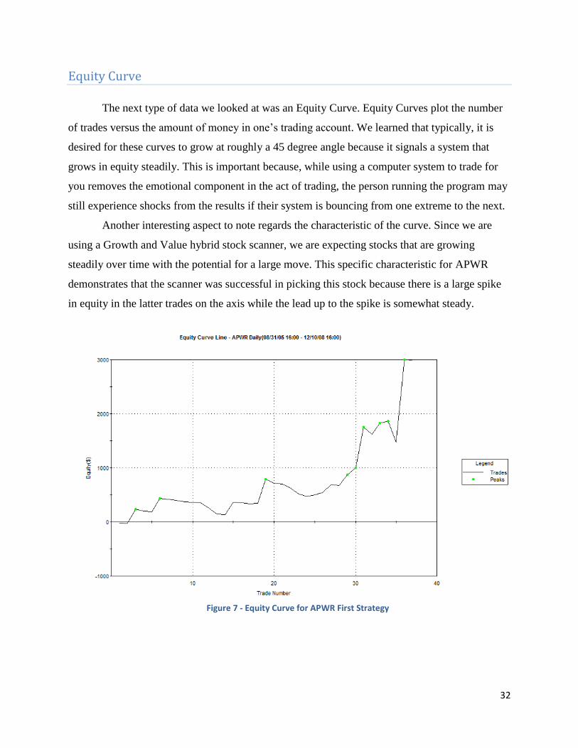
The next type of data we looked at was an Equity Curve. Equity Curves plot the number

of trades versus the amount of money in one‟s trading account. We learned that typically, it is

desired for these curves to grow at roughly a 45 degree angle because it signals a system that

grows in equity steadily. This is important because, while using a computer system to trade for

you removes the emotional component in the act of trading, the person running the program may

still experience shocks from the results if their system is bouncing from one extreme to the next.

Another interesting aspect to note regards the characteristic of the curve. Since we are

using a Growth and Value hybrid stock scanner, we are expecting stocks that are growing

steadily over time with the potential for a large move. This specific characteristic for APWR

demonstrates that the scanner was successful in picking this stock because there is a large spike

in equity in the latter trades on the axis while the lead up to the spike is somewhat steady.

Figure 7 - Equity Curve for APWR First Strategy

33

Trade Efficiency Graph

The next graph we looked at was the Trade Efficiency Graph. This type of graph plotted

all of the trades that were made versus their efficiency, or in other words, their increase in value.

This provided us with a great overview because we could see the distribution. Big winning and

losing trades are characterized by trades being plotted on the extrema of the chart. We were

hoping for distributions that would have data points predominantly in the positive range of the

efficiency axis. An even more ideal distribution would have the points clustered in a narrow

range of percentages which would indicate steady growth. That would be the equivalent to the

Equity Curve with a 45 degree angle.

Figure 8 - Trade Efficiency Graph for APWR First Strategy

34

Periodical Returns Table

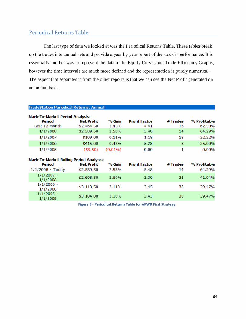
The last type of data we looked at was the Periodical Returns Table. These tables break

up the trades into annual sets and provide a year by year report of the stock‟s performance. It is

essentially another way to represent the data in the Equity Curves and Trade Efficiency Graphs,

however the time intervals are much more defined and the representation is purely numerical.

The aspect that separates it from the other reports is that we can see the Net Profit generated on

an annual basis.

Figure 9 - Periodical Returns Table for APWR First Strategy

35

At first, since this was our attempt at anything like this, we were pleasantly surprised and

a bit shocked at the results. Over a 4 year period, the system was able to generate $21,207 worth

of profit. We definitely were not anticipating that it would be this easy to generate a sizeable

profit. Our cautious optimism was quickly sobered when our advisor, Professor Radzicki,

explained that this occurrence was due probably to the fact that our strategy was effectively

curve fitted to each stock for the time period. Despite this, it was acknowledged that the results

were decent considering such a simple strategy because normally it takes a few iterations to

break even.

To deal with potentially skewing future results with curve fitting, we learned of a method

that we could apply once we refined our overall strategy. The method, out-of-sample testing, will

be introduced and explained in the Volume Exit Section where it was first applied.

First Strategy Summary Tables

This section presents two tables summarizing key results for quick reference. The first is

of optimized variables for each stock.

Table 6 - First Strategy Optimized Variables

First Strategy Optimized

Variables

Stock Symbol Slength Llength

APWR 18 19

CLMT 6 4

JST 41 42

NEU 12 7

NGLS 2 4

NRGP 34 34

NXG 44 44

KGS 1 1

36

Next is a table summarizing the number of trades, net profit, and profit factor for each

stock. These results would go on to be our baseline reference to compare to when analyzing the

results of new strategies. Values highlighted in red indicate a loss.

First Strategy Summary

Stock Symbol

Total Number of Trades

Total Net Profit

Profit Factor

APWR 37 $2,991.00 3.34

CLMT 132 $4,165.00 1.85

JST 72 $168.00 0.94

KGS 73 $615.00 1.21

NEU 185 $7,078.00 1.61

NGLS 83 $1,778.00 1.73

NRGP 43 $5,356.00 4.27

NXG 40 $608.00 0.30

Average 83.125 $2,650.88 1.91

Total 665 $21,207.00 Table 7 - First Strategy Results Summary

37

VI. The Volume Entry Strategy

This section of the report catalogs the formulation, testing, and results of the Volume

Entry Strategy applied to the stocks of the MAGNET Simple scanner.


The next strategy that we worked with was a modified version of the First Strategy that

incorporated a volume condition. During one of our meetings, we inquired about the role volume

played in the stock market and Professor Radzicki described it as “the number of votes in favor

of a move in price” and so, the more volume that is generated, the greater the chance of a larger

sustained move. The traditional definition of volume is the number of shares of a stock that are

traded in a given period of time. Adding a volume condition to the strategy entry would allow for

more selective entries, ensuring the strategy would not be in the market unless the volume of that

bar was greater than a number of bars ago. Therefore, we hypothesized that incorporating the

variable would lead to larger net profits since we increased the odds that we would enter during a

time frame during which there was a greater chance of a sustained move in price. For this first

study involving volume, we held our exit constant and only fine tuned the entry strategy so that

we could more accurately compare it to our First Strategy.

6.2 – Easy Language Code

The coding for this strategy simply involved adding an additional condition to the entry

strategy. Thus, we had to label a new variable that we would be optimizing. Upon searching

through TradeStation functions, not surprisingly, the Volume function came up as the one we

wanted to use for this approach. The following is the code for our Volume Entry Strategy:

Input: Slength(15), Llength(15), Vlength(15); if High > High[Llength] and Close > Close[Llength] and Volume > Volume[Vlength] then buy next bar at market; if Low < Low[Slength] and Close < Close[Slength] then sell short next bar at market;

38

6.3 - Tests

We tested this strategy in the same fashion as the First Strategy using exhaustive

optimization. „Vlength‟ was the same type of variable as the initial two and so all that was

needed was to select the range of values that we would test it for. Since volume is a much more

locally sensitive variable than past closes, highs, and lows, the range for the variable was set to

be between 1 to 15 bars instead of the 1 to 50 range for „Slength‟ and „Llength‟. Once again, the

date range was held constant between 12/10/2004 to 12/10/2008 to allow us to accurately

compare the outcomes between our two existing strategies. Additionally, a commission of $7.50

per trade was included. With the addition of a third variable, the number of tests increases from

2,500 to 37,500. A table is included for quick reference.

Variable Value

Date Range 12/10/2004 to 12/10/2008



Slength 1 to 50

Llength 1 to 50

Vlength 1 to 15

Tests: 37,500

Table 8 - Volume Entry Parameter Test Summary

6.4 - Results

Our hypothesis that including a volume variable in the entry conditions would increase

profit was proven correct. In the end, this set of tests concluded with only one stock being at a

net deficit. Also, the net profit for many of the other stocks was increased and the strategy ended

with an overall net of $31,405. This is a 48.09% increase in efficiency over the First Strategy.

Another important fact to note is that this strategy made 448 trades, which is less than the First

Strategy. In the Strategy Basis section, we hypothesized that there would be fewer trades due to

39

the selectiveness of the new entry conditions. These results were consistent with our

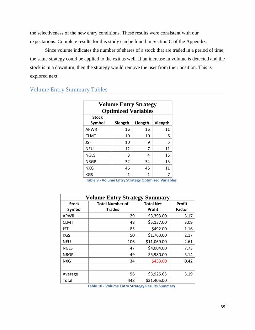
expectations. Complete results for this study can be found in Section C of the Appendix.

Since volume indicates the number of shares of a stock that are traded in a period of time,

the same strategy could be applied to the exit as well. If an increase in volume is detected and the

stock is in a downturn, then the strategy would remove the user from their position. This is

explored next.

Volume Entry Summary Tables

Volume Entry Strategy

Optimized Variables

Stock Symbol Slength Llength Vlength

APWR 16 16 11

CLMT 10 10 6

JST 10 9 5

NEU 12 7 11

NGLS 3 4 15

NRGP 32 34 15

NXG 46 45 11

KGS 1 1 7 Table 9 - Volume Entry Strategy Optimized Variables

Volume Entry Strategy Summary

Stock Symbol


Total Net Profit

Profit Factor

APWR 29 $3,393.00 3.17

CLMT 48 $5,137.00 3.09

JST 85 $492.00 1.16

KGS 50 $1,763.00 2.17

NEU 106 $11,069.00 2.61

NGLS 47 $4,004.00 7.73

NRGP 49 $5,980.00 5.14

NXG 34 $433.00 0.42

Average 56 $3,925.63 3.19

Total 448 $31,405.00 Table 10 - Volume Entry Strategy Results Summary

40

VII. The Volume Exit Strategy

This section of the report catalogs the formulation, testing, and results of the Volume Exit



The Volume Exit Strategy continues to build upon the success previous strategies. With

what we felt to be a solid entry in place, we proceeded towards developing our exit strategy. The

first exit strategy that we tried incorporated a volume condition. With the entry strategy turning

out the way it did, we hypothesized that taking the same approach with the exit might lead to

even better results. Like the volume entry, adding a volume exit condition would make for more

selective exits. This could be a double edged sword though because we might stay in longer if

the stock is moving too slowly and be trapped in a slow downtrend. On the other hand, if there

was sufficient volume, we would be exiting the market more often, thus giving us more

opportunities to enter. Nonetheless, while it is a relatively simple minded approach, we felt it

was worth trying before moving onto some more complex exits at the advice of our advisor.

7.2 - Easy Language Code

The coding for this strategy mimicked the previous section and to accomplish the desired

goal, we needed to add an additional condition to the exit. To differentiate between volume

variables, we labeled the entry „VElength‟ and the exit „VXlength‟. The following code was

complied:

Input: Slength(15), Llength(15), VElength(15), VXlength(15); if High > High[Llength] and Close > Close[Llength] and Volume > Volume[VElength] then buy next bar at market; if Low < Low[Slength] and Close < Close[Slength] and Volume > Volume[VXlength] then sell short next bar at market;

41

7.3 - Tests

With our strategy becoming more defined, we began to test more comprehensively. For

the first two studies, we were curve fitting our results to maximize our base profit. This is

referred to as in-sample testing. In our exit tests, we started off by performing in-sample testing

and then performed a second test by applying the results of the previous test to a different,

partially untested, time frame. This testing method is referred to as testing out-of-sample. It is an

intermediary step towards running the system on real time data. As in previous tests, the curve

fitting date range, commission charge and position size will be held constant. The new variable

„VXlength‟ will be tested over the same range as „VElength‟ of 1 to 15. With the addition of now

a fourth variable, the number of tests increases from 37,500 to 562,500! The date range for the

second test was 12/10/2007 to 12/10/2009. Tables are included for quick reference.

Variable Value

Date Range 12/10/2004 to 12/10/2008



Slength 1 to 50

Llength 1 to 50

VElength 1 to 15

VXlength 1 to 15

Tests: 562,500

Table 11 - Volume Exit Strategy Parameter In-Sample-Test Summary

42

Variable Value

Date Range 12/10/2007 to 12/10/2009



Slength Using values obtained in the Test 1

optimization. Llength

VElength

VXlength

Table 12 - Volume Exit Strategy Parameter Out-of-Sample Test Summary

7.4 - Results

In this study, our hypothesis that extending the volume condition to the exit strategy

would increase profits was supported. This set of tests concluded with all stocks being profitable

except for NXG. The same outcome occurred in the previous two studies. Once again, the net

profit for many of our scanner‟s stocks was enhanced further leading to an overall net of

$39,773. This is a 26.64% increase over the Volume Entry Strategy and an 87.54% increase over

the First Strategy. Based on these results we concluded that Volume plays an essential rule in

trading since the results were improved by such a staggering margin.

The number of trades made by this system for the 2004 to 2008 time interval was 529

which ended up being higher than the previous system‟s 448 trades. We were somewhat

expecting fewer trades to occur since adding another condition makes the exit more specific and

thus less common.

The last set of results involves applying the 2004-2008 optimized variables to the out of

sampled time range of 2007-2009. The system managed to generate $16,987 worth of profit over

2 years. We thought that this was very good considering that 2008 was an extremely rough year

for the markets due to the housing crisis. These results would now go on to be our baseline for

future comparisons and from here on out we would only be changing the exit strategy since that

is typically more difficult that determining and entry point. Comprehensive results for this study

can be found in Sections D and E of the Appendix

43

Volume Exit Summary Tables

Volume Exit Strategy Optimized

Variables

Stock Symbol Slength Llength VElength Vxlength

APWR 12 19 2 9

CLMT 3 2 1 8

JST 17 4 10 8

NEU 19 7 9 15

NGLS 1 11 15 4

NRGP 8 6 11 12

NXG 23 21 10 1

KGS 41 1 7 2 Table 13 - Volume Exit Strategy Optimized Variables

Volume Exit Strategy Summary (2004-2008)

Stock Symbol


Total Net Profit

Profit Factor

APWR 55 $4,598.00 5.43

CLMT 74 $5,459.00 2.30

JST 121 $4,215.00 2.00

KGS 39 $2,502.00 4.00

NEU 84 $12,478.00 3.95

NGLS 44 $3,596.00 5.15

NRGP 66 $7,159.00 5.25

NXG 46 $234.00 0.69

Average 66.125 $4,971.63 3.60

Total 529 $39,773.00 Table 14 - Volume Exit Strategy Results Summary (2004-2008)

44


Stock Symbol


Total Net Profit

Profit Factor

APWR 36 $3,339.00 3.26

CLMT 48 $3,495.00 3.04

JST 70 $1,612.00 1.31

KGS 46 $1,771.00 2.06

NEU 28 $3,825.00 1.83

NGLS 63 $1,138.00 1.47

NRGP 29 $2,000.00 1.94

NXG 20 $193.00 0.59

Average 42.5 $2,123.38 1.94


45

VIII. The LeBeau Exit Strategy

This section of the report catalogs the formulation, testing, and results of the LeBeau Exit



For our next study, we tested the LeBeau Exit Strategy at the recommendation of our

advisor. The LeBeau Exit Strategy is a complex system involving three different exit strategies

working in tandem. It was created by Charles “Chuck” LeBeau, who is a successful systematic

trader of stocks and futures. He has been active for over 40 years. More on Chuck LeBeau and

his strategies can be found on his website7. Since it is an exit strategy, we would be maintaining

our Volume Entry Strategy and rotate out our Volume Exit Strategy for the LeBeau Exit

Strategy. Before pursuing any tests, some outside reading and research was required in order to

even begin understanding how some of the functions were working. We were not sure what kind

of results we were to expect upon applying the strategy. In fact, the only real hypothesis we

could draw was whether or not this massive leap in system complexity would result in greater

profits.


The code for this strategy had been adapted to EasyLanguage and was supplied to us by

our advisor. It can be found in Section A of the Appendix as it spans multiple pages. Through our

research we were able to gain a basic understanding of some of the functions and operations that

were occurring within this strategy.

For starters, the LeBeau Strategy includes three different exits: Chandelier, Yo Yo, and

Modified Parabolic. According to the LeBeau PDF file, to understand the Chandelier and Yo Yo

exits an understanding of the Average True Range (ATR) is necessary.

The Average True Range (ATR) is the largest of the following three calculations: (1) The

difference between today's high and today's low. (2) The difference between today's high and

yesterday's close. (3) The difference between today's low and yesterday's close. The ATR is

7 http://www.traderclub.com/

46

always considered to be a positive value. From what can be seen, this value is possible to be

added as an indicator to a chart within TradeStation.

The Chandelier Exit is a trailing exit that changes as the high changes. This exit is

effective because it hangs down from the high price of the trade and moves up proportionally

whenever a new high is made. The "chain" on the Chandelier exit will contract and expand

slightly as the ATR adjusts to changes in volatility. The Chandelier exit usually starts new trades

with the default ATR of 3 (High minus 3 ATRs).

The Yo Yo Exit is a supplemental exit and cannot be used as a primary exit strategy. The

Yo Yo exit indicates when your position is on the wrong side of the market by identifying

abnormal volatility in the wrong direction. This exit is usually set at 2 ATRs below the most

recent close.

Modified Parabolic Exit is a trailing stop that moves closer and closer to the recent price

as new highs are made. According to LeBeau, the Unmodified Parabolic Exit is too sensitive and

exits too soon, thus the need for the Modified Parabolic Exit. These Parabolic Exits are based

upon the work of Welles Wilder in his book, New Concepts in Technical Trading8. The

Acceleration Factor (AF) is set to .02 and it is recommended to try .01 or .015 instead.

Setting profit targets within LeBeau's exit strategies are done using the Average

Directional Index (ADX), which is another concept introduced by Welles Wilder. When the

ADX is on the rise, patience is a virtue and large profits should be expected and vice versa

(Large is 4 ATR or more, Small is 1 or 2 ATR).

8 http://www.marketmasters.com.au/86.0.html

47

8.3 - Tests

We would proceed to test this strategy using the same method as in the previous section

where we optimized the variables and then tested out of sample. For our entry variables

„Slength‟, „Llength‟, and „Vlength‟, we would be using the same ranges as before. Concerning

the LeBeau variables, we initially did not know what range to optimize for. Searching on the

TradeStation Forums, we found some recommended values for some of the variables and upon

looking at the code, we found those values to already be inputted. Based on this, we concluded it

would be best to leave the LeBeau variables as they were and did not optimize for any of them.

Furthermore, including them may have resulted in days worth of optimizations being required for

each stock. This conclusion was based on the fact that just 4 variables required over 565,000

tests taking up a good portion of the day. Even adding one more variable at a range of 1-15

resulted in a grand total of 8,437,500 tests. We quickly realized that for complex trading systems,

time was a huge factor. TradeStation has a tool to speed such optimizations up through use of a

genetic algorithm. However, for our project, it was preferred that we stick with exhaustive

optimizations because they were pinpoint accurate and repeatable while genetic optimizations

were estimations.

Variable Value

Date Range 12/10/2004 to 12/10/2008



Slength 1 to 50

Llength 1 to 50

Vlength 1 to 15

LeBeau Variables Held at values in code.

Tests: 37,500

Table 16 - LeBeau Exit Strategy Parameter In-Sample-Test Summary

48

Variable Value

Date Range 12/10/2004 to 12/10/2008





Vlength


Tests: 37,500

Table 17 - LeBeau Exit Strategy Parameter Out-of-Sample Test Summary

8.4 – Results

The results for this study were somewhat disappointing. Considering the background and

complexity of the strategy, we were hoping for at least comparable net profits if not better. It

went to show that complex does not necessarily mean better. Over the optimized 4 year range in

the first test, the LeBeau Exit Strategy only netted $7,254 which was abysmally lower than the

Volume Exit Strategy. It also had three stocks at an overall net loss. When applied in the Out-of-

Sample test, it netted $7,099. Overall, it also had less activity than any previous system we‟ve

used before conducting only 377 and 226 trades. Another noteworthy result was that all of the

„Slength‟ values were 1. It was a curious trend, though not something we were able to find the

answer to. Due to the poor level of profit generated, it was later conjectured that there may have

been an incompatibility between the types of stocks that the MAGNET Scanner and the types of

stocks that the LeBeau Exit Strategy typically traded. This did not deter us from our next test

though. We sought to see if we could improve the LeBeau exit with some minor modifications.

Comprehensive results for this study are contained in Sections G and H of the Appendix.

49

LeBeau Exit Summary Tables

LeBeau Exit Strategy

Optimized Variables


APWR 1 19 5

CLMT 1 33 6

JST 1 6 4

NEU 1 12 53

NGLS 1 2 5

NRGP 1 17 15

NXG 1 6 4

KGS 1 16 14 Table 18 - LeBeau Exit Strategy Optimized Variables

LeBeau Exit Strategy Summary (2004-2008)

Stock Symbol


Total Net Profit

Profit Factor

APWR 57 $1,523.00 2.12

CLMT 42 $131.00 0.95

JST 70 $774.00 1.29

KGS 10 $345.00 0.29

NEU 63 $5,886.00 2.07

NGLS 19 $278.00 1.41

NRGP 54 $276.00 1.12

NXG 62 $1,007.00 0.08

Average 47.125 $906.75 1.17

Total 377 $7,254.00 Table 19 - LeBeau Exit Strategy Results Summary (2004-2008)

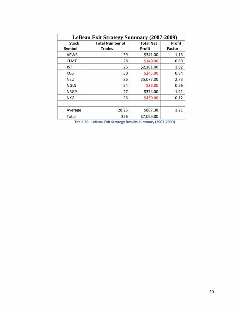
50

LeBeau Exit Strategy Summary (2007-2009)

Stock Symbol


Total Net Profit

Profit Factor

APWR 39 $341.00 1.13

CLMT 28 $140.00 0.89

JST 26 $2,161.00 1.82

KGS 30 $245.00 0.84

NEU 26 $5,077.00 2.73

NGLS 24 $39.00 0.96

NRGP 27 $374.00 1.21

NXG 26 $430.00 0.12

Average 28.25 $887.38 1.21

Total 226 $7,099.00 Table 20 - LeBeau Exit Strategy Results Summary (2007-2009)

51

IX. The LeBeau Short Exit Strategy

This section of the report catalogs the formulation, testing, and results of the LeBeau

Short Exit Strategy applied to the stocks of the MAGNET Simple scanner.


In this study, we sought to try and improve the LeBeau Exit Strategy. Through inspecting

the code, we found that it used a regular sell function. In most of our tests, we have been using

short selling as our exit from the market to decent success. Therefore it was hypothesized that we

could potentially improve the LeBeau Exit Strategy by changing instances of selling to short

selling.


Below is the isolated portion of the LeBeau Exit code that we edited. We found the

section of code we were interested in under Exits. We then proceeded to change all instances of

„sell‟ to „sell short‟.

//***** Exits *****

if Market_Position = 1 then

begin

if Chandelier_Touched >= Times_Touched then

Sellshort ( "LX_Cdlr" ) currentshares shares next bar at Chandelier_Stop STOP ;

if YoYo_Touched >= Times_Touched then

Sellshort( "LX_YoYo" ) currentshares shares next bar at YoYo_Stop STOP ;

Sellshort ( "LX_Pblc" ) currentshares shares next bar at Parabolic_Stop STOP ;

52

9.3 - Tests

The tests performed in this study are identical to the ones done in the previous study.

Tables are provided for quick reference and completeness.

Variable Value

Date Range 12/10/2004 to 12/10/2008



Slength 1 to 50

Llength 1 to 50

Vlength 1 to 15


Tests: 37,500

Table 21 - LeBeau Short Exit Strategy Parameter In-Sample-Test Summary

Variable Value

Date Range 12/10/2004 to 12/10/2008





Vlength


Tests: 37,500

Table 22 - LeBeau Short Exit Strategy Parameter Out-of-Sample Test Summary

53

9.4 - Results

Based on the generated results of the tests, we found that we were in fact able to make the

LeBeau Exit slightly better with the incorporation of short selling in the exit code. Compared to

the original version, the short version netted $3,091 or 42.61% more in the optimization, and

$5,904 or 83.17% more in the out-of-sample testing. So far through all of our studies, short

selling has proven to be a pretty strong method for exiting the market. This might be the case

considering the financial crisis. With the economy unstable as it is, a lot of equities have the

potential to tank and so we are constantly betting on things taking a dive and reacting as such in

our strategies. Contrary to the regular Lebeau Exit, this strategy experienced much more activity

conducting 768 trades through the optimized 4 year period and 440 trades in the out-of-sample

period. It tended to take heavier losses from stocks, but those were offset by larger gains in

others. Once again, the all the „Slength‟ values ended up being 1. We have not been able to find

an explanation for this occurrence yet. Comprehensive results for this study are contained in

Sections I and J of the Appendix.

LeBeau Exit Summary Tables

LeBeau Short Exit Strategy

Optimized Variables


APWR 1 38 2

CLMT 1 32 6

JST 1 46 8

NEU 1 13 10

NGLS 1 3 9

NRGP 1 48 4

NXG 1 10 4

KGS 1 16 14 Table 23 - LeBeau Short Exit Strategy Optimized Variables

54

LeBeau Short Exit Strategy Summary (2004-

2008)

Stock Symbol


Total Net Profit

Profit Factor

APWR 96 $2,515.00 2.15

CLMT 98 $743.00 1.15

JST 160 $3,467.00 1.59

KGS 22 $355.00 0.55

NEU 118 $7,735.00 1.76

NGLS 48 $117.00 1.05

NRGP 102 $2,180.00 0.67

NXG 124 $1,697.00 0.20

Average 96 $1,293.13 1.14

Total 768 $10,345.00 Table 24 - LeBeau Short Exit Strategy Results Summary (2004-2008)

LeBeau Short Exit Strategy Summary (2007-

2009)

Stock Symbol


Total Net Profit

Profit Factor

APWR 52 $537.00 1.24

CLMT 58 $995.00 0.68

JST 52 $7,429.00 4.52

KGS 62 $1,794.00 0.41

NEU 48 $8,531.00 2.70

NGLS 54 $214.00 1.08

NRGP 51 $122.00 1.04

NXG 63 $1,041.00 0.14

Average 55 $1,625.38 1.48

Total 440 $13,003.00 Table 25 - LeBeau Short Exit Strategy Results Summary (2007-2009)

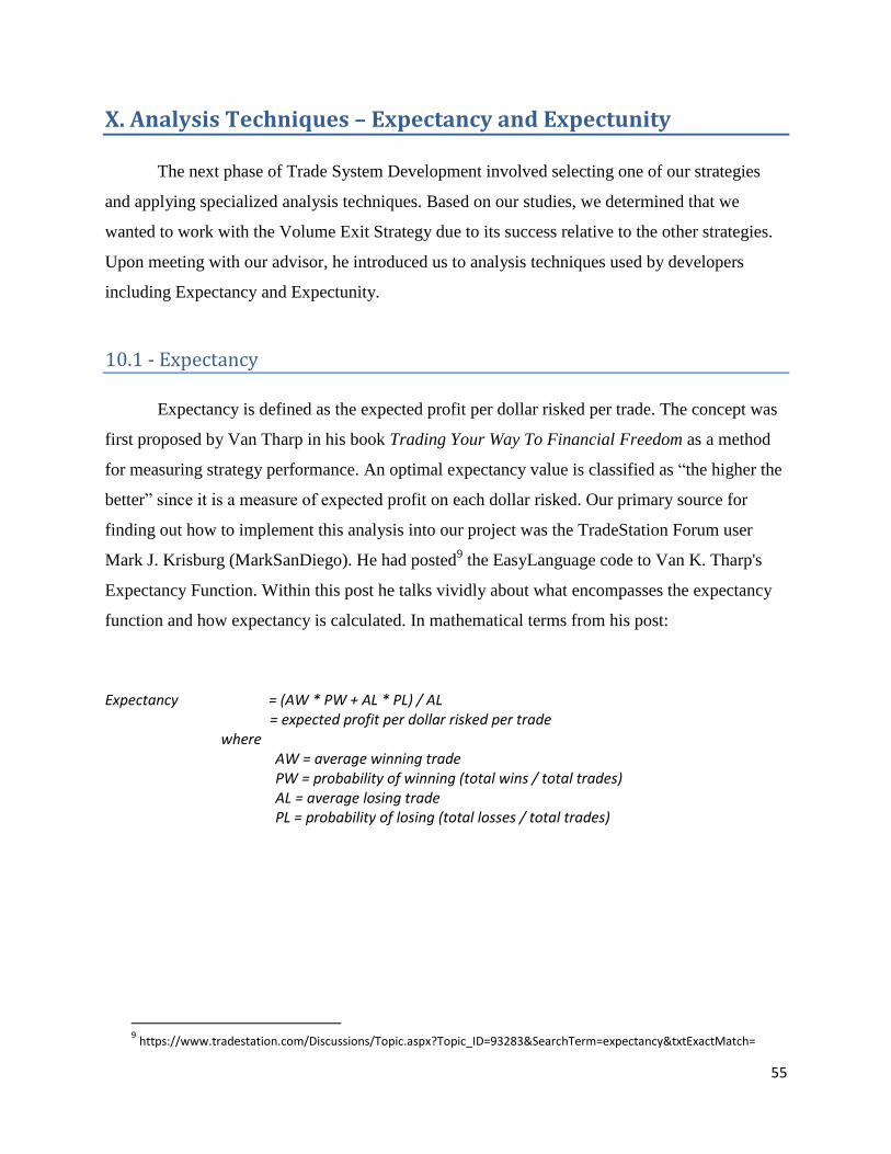
55

X. Analysis Techniques – Expectancy and Expectunity

The next phase of Trade System Development involved selecting one of our strategies

and applying specialized analysis techniques. Based on our studies, we determined that we

wanted to work with the Volume Exit Strategy due to its success relative to the other strategies.

Upon meeting with our advisor, he introduced us to analysis techniques used by developers

including Expectancy and Expectunity.

10.1 - Expectancy

Expectancy is defined as the expected profit per dollar risked per trade. The concept was

first proposed by Van Tharp in his book Trading Your Way To Financial Freedom as a method

for measuring strategy performance. An optimal expectancy value is classified as “the higher the

better” since it is a measure of expected profit on each dollar risked. Our primary source for

finding out how to implement this analysis into our project was the TradeStation Forum user

Mark J. Krisburg (MarkSanDiego). He had posted9 the EasyLanguage code to Van K. Tharp's

Expectancy Function. Within this post he talks vividly about what encompasses the expectancy

function and how expectancy is calculated. In mathematical terms from his post:

Expectancy = (AW * PW + AL * PL) / AL = expected profit per dollar risked per trade where AW = average winning trade PW = probability of winning (total wins / total trades) AL = average losing trade PL = probability of losing (total losses / total trades)

9 https://www.tradestation.com/Discussions/Topic.aspx?Topic_ID=93283&SearchTerm=expectancy&txtExactMatch=

56

EasyLanguage Code

Based off of his post, we were eventually able to construct the code required to calculate

the expectancy of our strategy over our set of stocks. In the process, we experienced a number of

difficulties that led us in having to contact Mr. Krisburg. A transcript of our exchanges with him

can be found in Section K of the Appendix. Ultimately the following code was applied to our

trading system:

Input: slength(15), Llength(15),VElength(15),VXlength(15); vars: int TradingDays(0), float oExpectPerTrade(0), float oExpectancy(0); //buy if High > High[Llength] and Close > Close[Llength] and Volume > Volume[VElength] then buy next bar at market; //sell if Low < Low[Slength] and Close < Close[Slength] and Volume > Volume[VXlength] then sell short next bar at market; { within calling strategy } if Date <> Date[1] then TradingDays = TradingDays + 1; if LastBarOnChart then begin value1 = _Expectancy(TradingDays, oExpectPerTrade, oExpectancy); end; Print("ExpectancyPerTrade: ", oExpectPerTrade, " Expectancy: ", oExpectancy);

This code relies on another function, _Expectancy, which needed to be imported into

TradeStation. The EasyLanguage code for this function can be referenced in Section A of the

Appendix.

57

Results

The results in Table 26 below summarize the results of this analysis. Expectancy per Trade and

Expectancy are both outputs from the applied function. In comparing the Expectancy values to

the Total Net Profit from the Volume Exit Strategy, it can be seen that there is a relationship. The

stocks NEU and NRGP were the most profitable for that strategy and this is reflected in these

stocks having the two highest expectancy values in the set.

Stock Symbol

Number of Trades

Expectancy Per Trade Expectancy

APWR 68 2.12 38.29

CLMT 99 0.75 20.09

KGS 71*10 0.89 29.17

JST 161 0.46 15.46

NEU 199 1.05 43.63

NGLS 56 1.03 21.76

NRGP 164 0.95 36.68

NXG 34 -0.07 -0.48 Table 26 - Expectancy per Stock

10.2 - Expectunity

Expectunity, another function created by Van Tharp, is a variation of Expectancy. It is a

combination of Expectancy and Opportunities, which are the number of possible trades in a year.

The definition for Expectunity is the expected return for each dollar risked per opportunity.

Formulation

Unlike Expectancy, Expectunity is an analysis that is better done on a Microsoft Excel

Spreadsheet. Since we already had the Expectancy values calculated from before, we needed to

define and calculate Opportunities. Research led us to find that:

𝑂𝑝𝑝𝑜𝑟𝑡𝑢𝑛𝑖𝑡𝑖𝑒𝑠 = # 𝑜𝑓 𝑇𝑟𝑎𝑑𝑒𝑠 ∗ 365

𝑆𝑡𝑢𝑑𝑦 𝐷𝑎𝑦𝑠

10

Discrepancy in value, unable to repeat the 78 trades existent in the Performance Summary.

58

The fraction is the total days in a year divided by study days. Study days are the number

of possible trading days in a year multiplied by the duration of years that the study spans. The

number of trading days in one year was found to be 252. In our case, we were looking at the

window of time between 2004 and 2009, so our number of years was 5. This led to a total of

1260 study days.

Results

The following table summarizes the results of the variables and equations plugged into a

Microsoft Excel Spreadsheet. From this we could see that NEU and NRGP were stocks that

performed exceedingly well using our trading system.

Stock Symbol Expectancy

Number of Trades Opportunities Expectunity

APWR 38.29 68 19.70 754.25

CLMT 20.09 99 28.68 576.15

KGS 29.17 71*11 22.31 650.65

JST 15.46 161 46.64 721.04

NEU 43.63 199 57.65 2515.13

NGLS 21.76 56 16.22 353.00

NRGP 36.68 164 47.51 1742.59

NXG -0.48 34 9.85 -4.73 Table 27 - Expectunity per Stock

11

Discrepancy in value, unable to repeat the 78 trades existent in the Performance Summary.

59

XI. Miscellaneous Strategies and Other Works

This section is a catalog of attempted tests and coding done concurrently throughout the

project with some of the aforementioned chapters. Unfortunately for one reason or another, these

avenues did not see fruition or completion, but nonetheless deserve some sort of recognition.

Some of these sections will include partial transcripts of journal entries since they describe the

work done on the topic in the best manner and it has been a substantial amount of time since we

worked with some of them. While most topics in the overall report are covered in a very

straightforward and sometimes simple manner, this section will hopefully illustrate that things

were not always so easy and smooth sailing. There were a number of occasions where we would

hit blocks and be stalled for some periods of time while we tried to find solutions to our

problems.

11.1 - The Charlie Wright Coke Strategy

Early in our project, while we were determining which scanner to select, we started

working on understanding entry and exit strategies. One of these sets of strategies we worked

with was Charlie Wright‟s KO5 Strategy, which was the 5th

incarnation and most refined strategy

covered in his book we read, Trading as a Business. His code can be found in Section A of the

Appendix. While we did not extensively test this strategy, it played an important role early on in

our learning process where it gave us a strategy to apply and mess around with. The passage

below is a transcript of a journal entry concerning its use and a result.

October 26th - 30th 2009

… From here I decided to look into Charlie Wright's Coke strategy again on a weekly chart of AWPR (one of the results from the MAGNET Scan, randomly selected). Applying KO5 to the weekly chart produced 3 trades over the course of 2005-2009, 2 short trades and 1 long. A profit factor of 5.31, and a net profit of $478. Observing the weekly bar graph of AWPR from 2005-2009, it becomes obvious that KO5, even though it had a net profit, missed many trading opportunities due to not identifying shorts accurately. The Long trade appears like it could not have been made any better since the strategy was in the market during "the big one", but shorted to late and thus lost many potential profits. The shorting system will have to be looked at and possibly tweaked to better optimize it. This lack of shorting got me to thinking to better indicate on the chart where a bar of interest appears

60

using PaintBars and created "MyFirstPaintBar" after viewing the EasyLanguage introduction tutorial. With this, the chart will be colored red when a bar of interest appears (ex: when the close of the current bar is less than that of the past 10 bars). This can be very useful to determine where the trades should have occurred.

11.2 - Exit with a Profit/Exit with a Loss

At the point before we started incorporating volume conditions in our entry and exit

strategies, we did some work with some exit strategies that exit once a certain threshold has been

met. So, for example, if the trade had made or lost $100, it would exit immediately. It was only

partially successful and in the end we had two gripes with it. One of the problems that we had

with this strategy is that sometimes it would not initiate a sell. Another consisted of the fact that

it would sell and then never re-enter the market. At some points, we were able to get it to work

successfully, however it would then work contrary to our goals. Unfortunately, we were unable

to get the strategy to work positively and consistently, and as time progressed, this strategy was

laid on the backburner and we did not returned to it since we were having much greater

successes with our Volume Entry and Exit Strategies. The passages below are journal entries

cataloging the work done on this strategy as well as the code we used.

November 15th - 21st 2009 ... A crude model of a Exit with a Profit (Profit stop) was crafted. The results upon first glace appeared promising with only teal profit bars to be seen and no red loss bars. Upon examination of the strategy, a total net profit of $2,338 was reached with a $70 profit stop. The EasyLanguage code for this strategy is listed below: Inputs: slength(15), Llength(15),PositionBasis( false ), Amount( 100 ) ; if High > High[Llength] and Close > Close[Llength] then buy next bar at market; if PositionBasis then SetStopPosition; SetProfitTarget( Amount ) ; Upon examination of the code, it became quite clear as to why only profitable trades were noted, the only exit was a profit, and thus would hold onto the position until a profit of $70 was made, then it would exit. This brings up the important note that this is not to be a sole exit, but to be used in conjunction with a primary exit such as the short. The profit and loss stop exits are meant to be a secondary exit, where if the initial criteria is not reached, but the secondary is, it will exit to keep the best interest of the trader in mind.

61

A stop loss exit was also crafted, the code is listed below: Input: Llength(15), PositionBasis( false ), Amount( 1 ) ; if High > High[Llength] and Close > Close[Llength] then buy next bar at market; if PositionBasis then SetStopPosition else SetStopShare ; SetStopLoss( Amount ) ; This is meant to be a secondary exit to a primary short exit. What was noticed with this strategy is it would only sell once a loss of $100 was achieved.

November 22nd - 28th 2009

Stop Loss & Profit Loss The Stop Loss & Profit Loss were tested in conjunction with the newly formed Volume Entry Strategy as a way to ensure maximum profit. Even though these two strategies are meant to act as a fail safe to protect profits, they in turn hindered them. The Profit Loss strategy when optimized across APWR provided positive results, but there was an apparent error within both this strategy and the Stop Loss. It was noted that within both strategies, the number of trades have increased dramatically since the stop was being triggered quite often. Each time the stop triggered, the strategy reset itself in terms of what data to look at for entries and exits. This became a crucial error within this system as the strategy missed many crucial entry and exit points that would normally not have been avoided.

11.3 - Exchange-Traded Fund (ETF)

Another topic we worked with through our journey was ETF. In short terms, it is

something akin to a stock for an entire market sector and trades at about the same price as the net

asset value of the industry. In researching this topic, we were looking for ways to compare the

performance of an individual stock to the performance of the overall sector. This data could be

used in our scanner to return more selective results among other things. The following passage

summarizes our work on the topic.


ETF for Market Share This would be used for each market sector, an example would be comparing the price of Oil versus Exxon. If Oil is declining rapidly, it would not be wise to hold Exxon stock. To be able to model this in TradeStation, we would need to know what industries the stocks that are returned from the scan are. Adding the "Sector" filter to display in the MAGNET Scan. The sectors returned are Utilities, Technology, Basic Materials, Energy and Services.

62

A new strategy would have to be implemented for each sector, thus a strategy for: Basic Materials, Capital Goods, Conglomerates, Consumer Cyclical, Consumer / Non-Cyclical, Energy, Financial, Healthcare, Services, Technology, Transportation, Utilities. Each strategy would look at the sectors movement in comparison to the movement of the equity in question and if the price of the equity rose or remained constant while the sector declined, then it would be unwise to continue to hold a stake of that company. Upon first glance it would appear that ETF would be implemented on the strategy level, after searching the TradeStation Forums, EasyLanguage Dictionary and Help Center, this is not the case. The ETF command would be implemented on Scanner level, thus eliminating the need for a multitude of different strategies. It would appear that this could also be done on the Industry level, doing so would provide a less specific result though. Sector > Industry (Showing that the sector is outperforming the industry), decreases the list of potential stocks from 7 to 2. Sector < Industry, 5 results from 7 Sector >= Industry, 2 results form 7 Sector <= Industry, 5 results from 7 In theory this approach appears to be a solid reasoning for following or ignoring a stock by looking at its sector strength to its industry strength. But this does not give a specific of the stock itself, a sector could excel or decline in performance due to a couple outlining companies. Without a way to compare the equity to either the sector or the industry.

11.4 - The Chicago Board Options Exchange Volatility Index (VIX)

The VIX is another board exchange similar to ETFs that measures the volatility in prices

within the S&P 500. We were also looking for potential ways to incorporate its trends and results

into the strategies we were using but ran into an impassible wall. Unfortunately, acquiring access

to the VIX required an additional $10 to $55 per month in subscription fees. This was out of our

budget considering that this project was coming out of our own pocket. The following passage

contains our brief exploration of the exchange.


$VIX VIX, also known as the Chicago Board Options Exchange Volatility Index measures expectations of volatility or fluctuations in price within the S&P 500. Higher values of the Volatility Index indicate the outlook of investors. They believe that the S&P 500 will fluctuate greatly, but does not indicate direction

63

since it could be a dramatic profit or loss. For this reason, the Volatility Index is also known as the "Fear Index". Attempting to enter in the symbol VIX for the S&P Volatility Index or VXN for the Nasdaq Volatility Index within TradeStation both produced errors stating "No Symbol Found". After searching within the forums for some time, a post from 2008 started that (at that time TradeStation did not include these indices), another post listed the VIX index as the symbol $VIX.X entering this ticker into the Symbol/Lookup Bar produced an error "Data Request Failed: Account not enabled for this data". To access this feature within TradeStation it would cost an additional $10-$55 a month on top of the $29 currently for the service. The Volatility Index can still be viewed, just not within TradeStation, thus adding any measurable unbiased change to the strategy would not be possible, at least not with automation.

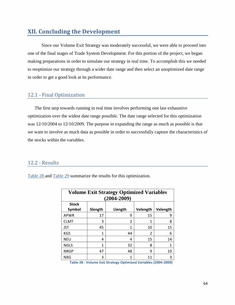
64

XII. Concluding the Development

Since our Volume Exit Strategy was moderately successful, we were able to proceed into

one of the final stages of Trade System Development. For this portion of the project, we began

making preparations in order to simulate our strategy in real time. To accomplish this we needed

to reoptimize our strategy through a wider date range and then select an unoptimized date range

in order to get a good look at its performance.

12.1 - Final Optimization

The first step towards running in real time involves performing one last exhaustive

optimization over the widest date range possible. The date range selected for this optimization

was 12/10/2004 to 12/10/2009. The purpose in expanding the range as much as possible is that

we want to involve as much data as possible in order to successfully capture the characteristics of

the stocks within the variables.

12.2 - Results

Table 28 and Table 29 summarize the results for this optimization.

Volume Exit Strategy Optimized Variables

(2004-2009)

Stock Symbol Slength Llength Velength Vxlength

APWR 17 9 15 9

CLMT 3 2 1 8

JST 45 1 10 15

KGS 1 44 2 6

NEU 4 4 15 14

NGLS 1 32 8 1

NRGP 47 48 9 10

NXG 3 1 11 3 Table 28 - Volume Exit Strategy Optimized Variables (2004-2009)

65


Stock Symbol


Total Net Profit

Profit Factor

APWR 68 $4,953.00 4.35

CLMT 99 $6,903.00 2.42

JST 161 $4,156.00 1.63

KGS 78 $2,902.00 2.36

NEU 199 $20,858.00 2.69

NGLS 56 $3,546.00 3.21

NRGP 164 $7,770.00 2.67

NXG 34 $64.00 0.91

Average 107.375 $6,378.00 2.53


12.3 - Real Time Simulation

Through the last stretch of our project, we ran our trading system in real time. To do this,

we performed an out-of-sample test where no date in the range had been included in any

optimizations. We applied the optimized variables in Table 28 to the date range: 12/10/2009 –

2/29/2010. In performing this simulation, no net profits were generated. However, it should be

noted that APWR entered the market on 2/26/2010 and NRGP entered the market on 2/25/2010.

Overall, this was at least somewhat promising for such a short time frame. Many of the stocks

have variables that are looking between 30 and 40 bars back and it is unreasonable to expect any

major gains in such a small time frame since there is a lack of data points.

66

12.4 - Going Further

The process one goes through in Trading System Development does not end here. As a

matter of fact, there are still a myriad of avenues one can take with their system. Below are two

topics that we did some preliminary work into, however could not complete because of the time

limit we had on the project.

Position Sizing

Another component of trade systems that we looked at while we were developing our

strategies was position sizing. As the reader recalls, we kept our shares per trade constant at 100.

Including position sizing code into our strategies would allow our system to change that value to

take advantage of situations based on the current value of the fund. Unfortunately, we ran into

another cost constraint with this as the license. The function called in the code that made position

sizing possible cost $299. Incidentally there existed a user created function that would have

allowed us to achieve the same ends, however it took too much time to acquire and we were not

able to successfully implement it before the end of the project.

Monte Carlo Analysis

Monte Carlo Analysis is a technical analysis through which one scrambles the order of the

trades that their trading system will encounter. Doing so allows the user to determine whether or

not the account traded will be wiped out with a string of unprofitable trades. Monte Carlo also

tells us the maximum number of losing trades in a row, thus if ran in real time and there were

five losing trades in a row and yet the maximum number possible in a row was seven, you would

have a frame of reference of where the absolute rock bottom was.

67

XIII. Closing Statement

Through the months of working on this project, we have come to develop an appreciation

for the method behind Trading System Development as well as TradeStation itself. At times, it

was a constant uphill struggle in order to get some functions to work properly, however

TradeStation still remains a powerful tool. In pursuing this methodology, we were able to

achieve each of our goals to some degree. We gained a number of insights into stock trading and

became familiar with a lot more terminology. We successfully learned how to use a few tools in

TradeStation, though it would seem there are still and endless amount to go through. We were

also able to successfully design and test a trading system scientifically and build it block by

block. Thus we were able to add value to the MAGNET Scanner by determining some viable

entry and exit strategies. We hope that our work demonstrates that the average user can

profitably create and trade on a trading system while utilizing the power of scanners to aide them

in their efforts.

68

Appendix

Section A: TradeStation Easy Language Code

My First Showme If High > High[15]

then Plot1(High); If Low < Low[15] then Plot2(Low);

My First Paintbar If Close > Average(Close,10) Then PlotPaintBar(High,Low);

Charlie Wright’s KO5 Input: AvgLen(30),PrctRLen(10), BuyLvl(20),SellLvl(80); IF CurrentBar > 1 and Average(Close,AvgLen) > Average(Close,AvgLen)[1] and PercentR(PrctRLen) crosses above 20 Then Buy("%R Buy") Next Bar at market; IF CurrentBar > 1 and Average(Close,AvgLen) < Average(Close,AvgLen)[1] and PercentR(PrctRLen) crosses below 80 Then Sell Short ("%R Sell") Next Bar at market; Sell Short ("LL") Next Bar at Lowest(low,50) - 1 point stop; Buy ("HH") Next Bar at Highest(high,50) + 1 point stop; If Date = 970725 and MarketPosition = 1 Then Sell Next Bar at Market; If Date = 970725 and MarketPosition = -1 Then Buy to Cover Next Bar at Market;

First Strategy Input: slength(15), Llength(15);

if High > High[Llength] and Close > Close[Llength] then buy next bar at market; if Low < Low[Slength] and Close < Close[Slength] then sell short next bar at market;

69

Volume Entry Strategy Input: slength(15), Llength(15), Vlength(15);

if High > High[Llength] and Close > Close[Llength] and Volume > Volume[Vlength] then buy next bar at market; if Low < Low[Slength] and Close < Close[Slength] then sell short next bar at market;

Volume Exit Strategy Input: slength(15), Llength(15), VElength(15), VXlength(15);

if High > High[Llength] and Close > Close[Llength] and Volume > Volume[VElength] then buy next bar at market; if Low < Low[Slength] and Close < Close[Slength] and Volume > Volume[VXlength] then sell short next bar at market;

Lebeu Exit Strategy Inputs: slength(15), Llength(15), Vlength(15), Chandelier_AvgRange (2.5), YoYo_AvgRange (2), Times_Touched (10), // MIT only if Chandelier and YoYo Parabolic_Accel_Factor (.01), // futures default -- for equities use 0.05 +- AvgRange_Length (21), Profit_AvgRange (1), Profit_Switch_Factor (0.6), Commentary_On ( False ) ; If High > High[Llength] and Close > Close[Llength] and Volume > Volume[Vlength] then buy next bar at market; VARIABLES: aChandelier_AvgRange( AbsValue( Chandelier_AvgRange ) ), // aYoYo_AvgRange ( AbsValue( YoYo_AvgRange ) ), // Parabolic_AF ( AbsValue( Parabolic_Accel_Factor ) ), // convert inputs to absolute value| aAvgRange_Length ( AbsValue( AvgRange_Length) ), // aProfit_AvgRange ( AbsValue( Profit_AvgRange ) ), // Acceleration_Factor ( Parabolic_AF ),

Parabolic_AF_Limit ( Parabolic_AF * 10 ), // set limit 10x factor Average_Range ( 0 ),

Market_Position ( 0 ), IntrabarPersist Trade_High ( 0 ), // highest high of current trade IntrabarPersist Trade_Low ( 0 ), // lowest low of current trade

70

YoYo_Amount ( 0 ) // YoYo stop amount YoYo_Price ( 0 ), // pin price to last bar close IntrabarPersist Chandelier_Stop ( 0 ), // IntrabarPersist YoYo_Stop ( 0 ), // stop prices Parabolic_Stop ( 0 ), // Profit_Amount ( 0 ), //

IntrabarPersist Profit_Switch ( False ), // point at which Chandalier Stop tightens

Not_Optimizing ( True ), GV_Name ( NumToStr( AbsValue( GetAppInfo( aiAppID ) ), 0 ) ), PT_On ( False ), // get from PT_MIT strategy IntrabarPersist Chandelier_Touched ( 0 ), IntrabarPersist YoYo_Touched ( 0 ), IntrabarPersist Bar_Number ( 0 ), PT_Range_Mult ( aProfit_AvgRange ), PT_Range_Length ( aAvgRange_Length ), PT_Average_Range ( 0 ), Avg_Entry_Price ( 0 ), aProfit_Switch_Fac ( AbsValue( Profit_Switch_Factor ) ), New_Entry ( False ) ;

//***** Housekeeping ***** if CurrentBar = 1 then

Not_Optimizing = GetAppInfo( aiOptimizing ) <> 1 ; //---------------------------------------------------------------------------------------------------------------------------------------| // This code gets the PT_MIT strategy settings to calculate the PT settings of the LeBeau | // Stops. If no PT_MIT present, then uses local LeBeau settings. | //---------------------------------------------------------------------------------------------------------------------------------------| if CurrentBar = 2 then

begin PT_Range_Mult = GVGetNamedDouble( GV_Name + "PT_Range_Mult", aProfit_AvgRange ) ; PT_Range_Length = GVGetNamedDouble( GV_Name + "PT_Range_Length", aAvgRange_Length ) ; if Not_Optimizing then begin Value1 = GVSetNamedDouble( GV_Name + "Chandelier_AvgRange", aChandelier_AvgRange ) ; Value2 = GVSetNamedDouble( GV_Name + "YoYo_AvgRange", aYoYo_AvgRange ) ; Value3 = GVSetNamedDouble( GV_Name + "Parabolic_AF", Parabolic_AF ) ;

71

Value4 = GVSetNamedDouble( GV_Name + "LeBeau_AvgRange_Length", aAvgRange_Length ) ; Value6 = GVSetNamedDouble( GV_Name + "Parabolic_AF_Limit",Parabolic_AF_Limit ) ;

Value5 = GVSetNamedDouble( GV_Name + "Profit_AvgRange", PT_Range_Mult ) ; Value7 = GVSetNamedDouble( GV_Name + "LePT_Range_Length", PT_Range_length ) ; Value8 = GVSetNamedDouble( GV_Name + "Profit_Switch_Factor", aProfit_Switch_Fac ) ; end ; // not optimizing end ; // 2nd bar housekeeping

//***** Compute Stops *****

Market_Position = MarketPosition ; // in order to access historical bar market position if BarStatus(1) = 2 then // calc only once per bar begin Average_Range = AvgRange( aAvgRange_Length ) ; Avg_Entry_Price = AvgEntryPrice ; New_Entry = Avg_Entry_Price[1] <> Avg_Entry_Price ; PT_Average_Range = AvgRange( PT_Range_Length ) ; Profit_Amount = Round( PT_Range_Mult * PT_Average_Range, 2 ) ; YoYo_Amount = aYoYo_AvgRange * Average_Range ; end // calc once else if Bar_Number <> CurrentBar then // calc on first tick of new bar formation begin Bar_Number = CurrentBar ; if Not_Optimizing and GetAppInfo( aiRealTimeCalc ) = 1 then begin Chandelier_Touched = 0 ; YoYo_Touched = 0 ; end // reset at end of bar if not optimizing else begin Chandelier_Touched = Times_Touched ; YoYo_Touched = Times_Touched ; end ; // if optimizing, set to limit end ; // reset touched each new bar if Market_Position[1] <> 0 then YoYo_Price = Close[1] else YoYo_Price = Open ; if Market_Position <> 0 then // eval market position on current bar

72

begin

//*** Long Position *** if Market_Position = 1 then begin if Market_Position[1] <> 1 or New_Entry then // eval market position on prior bar and reset variables if begin Profit_Switch = False ; // reset profit switch Trade_High = High ; // reset trade high end // reset else if High > Trade_High then // find new high Trade_High = High ; //* Chandelier Stop * if Profit_Switch or // if switch = true Trade_High >= AvgEntryPrice + ( Profit_Amount * aProfit_Switch_Fac ) then begin Profit_Switch = True ; Chandelier_Stop = Round( Trade_High - ( aChandelier_AvgRange *

Average_Range * aProfit_Switch_Fac ), 2 ) ; // tighten stop end // tighten Chandelier stop when profit point exceeded else Chandelier_Stop = Round( Trade_High - ( aChandelier_AvgRange * Average_Range ), 2 ) ;

// normal stop if Market_Position[1] = 1 and New_Entry = False and Chandelier_Stop < Chandelier_Stop[1] then Chandelier_Stop = Chandelier_Stop[1] ; // prevent retracement if Close <= Chandelier_Stop then Chandelier_Touched = Chandelier_Touched + 1 ; //* YoYo Stop * YoYo_Stop = Round( YoYo_Price - YoYo_Amount, 2 ) ; if Close <= YoYo_Stop then YoYo_Touched = YoYo_Touched + 1 ; //* Parabolic Stop * if Market_Position[1] <> 1 or

73

New_Entry then begin Parabolic_Stop = Chandelier_Stop ; // initial setting Round( AvgEntryPrice - ( aChandelier_AvgRange *

Average_Range ), 2 ) ; // tie to entry price Acceleration_Factor = Parabolic_AF ; end // eval market postion on prior bar else begin {if BarStatus(1) = 2 then begin} if Trade_High > Trade_High[1] and Acceleration_Factor < Parabolic_AF_Limit then Acceleration_Factor =

Acceleration_Factor + MinList( Parabolic_AF, Parabolic_AF_Limit - Acceleration_Factor ) ; Parabolic_Stop = Parabolic_Stop + Acceleration_Factor * (

Trade_High - Parabolic_Stop ) ; if Parabolic_Stop > Low then // force stop <= low of last bar Parabolic_Stop = Low ; {end ;} // update only at end of bar end ; // long parabolic stop end // long market postion //*** Short Position *** else begin // short market position if Market_Position[1] <> -1 or New_Entry then // eval market position on prior bar begin Profit_Switch = False ; // reset profit switch Trade_Low = Low ; // reset trade low end else if Low < Trade_Low then // find new low Trade_Low = Low ; //* Chandelier Stop * if Profit_Switch or // if switch = true Trade_Low <= AvgEntryPrice - ( Profit_Amount * aProfit_Switch_Fac ) then begin Profit_Switch = True ;

74

Chandelier_Stop = Round( Trade_Low + ( aChandelier_AvgRange * Average_Range * aProfit_Switch_Fac ), 2 ) ; // tighten stop

end // tighten Chandelier stop when profit point exceeded else Chandelier_Stop = Round( Trade_Low + ( aChandelier_AvgRange * Average_Range ), 2 ) ;

// normal stop if Market_Position[1] = -1 and New_Entry = False and Chandelier_Stop > Chandelier_Stop[1] then Chandelier_Stop = Chandelier_Stop[1] ; // prevent retracement if Close >= Chandelier_Stop then Chandelier_Touched = Chandelier_Touched + 1 ; //* YoYo Stop * YoYo_Stop = Round( YoYo_Price + YoYo_Amount, 2 ) ; if Close >= YoYo_Stop then YoYo_Touched = YoYo_Touched + 1 ; //* Parabolic Stop * if Market_Position[1] <> -1 or New_Entry then begin Parabolic_Stop = Chandelier_Stop ; Round( AvgEntryPrice + ( aChandelier_AvgRange * Average_Range ),

2 ) ; // tie to entry price Acceleration_Factor = Parabolic_AF ; end // eval market postion on prior bar else begin {if BarStatus(1) = 2 then begin} Parabolic_Stop = Parabolic_Stop + Acceleration_Factor * ( Trade_Low

- Parabolic_Stop ) ; if Trade_Low < Trade_Low[1] and Acceleration_Factor < Parabolic_AF_Limit then Acceleration_Factor = Acceleration_Factor +

MinList( Parabolic_AF, Parabolic_AF_Limit - Acceleration_Factor ) ; if Parabolic_Stop < High[1] then Parabolic_Stop = High[1] ; {end ;} // only once per bar

75

end ; // short parabolic stop end ; // short market position //***** Exits ***** if Market_Position = 1 then begin if Chandelier_Touched >= Times_Touched then Sell ( "LX_Cdlr" ) currentshares shares next bar at Chandelier_Stop STOP ; if YoYo_Touched >= Times_Touched then Sell( "LX_YoYo" ) currentshares shares next bar at YoYo_Stop STOP ; Sell ( "LX_Pblc" ) currentshares shares next bar at Parabolic_Stop STOP ; end // long stops else begin if Chandelier_Touched >= Times_Touched then BuyToCover ( "SX¯Cdlr" ) currentshares shares next bar at Chandelier_Stop STOP ; if YoYo_Touched >= Times_Touched then BuyToCover ( "SX¯YoYo" ) currentshares shares next bar at YoYo_Stop STOP ; BuyToCover ( "SX¯Pblc" ) currentshares shares next bar at Parabolic_Stop STOP ; end ; // short stops end ; // set stops -- MarketPostion <> 0

//***** Commentary ***** if Commentary_On and AtCommentaryBar then Commentary( ( Date - ( Year( Date ) * 10000 ) ):0:0, Time:5:0, " -- BarNumber = ", CurrentBar:5:0, NewLine, "High = ", High, NewLine, "Low = ", Low, NewLine, "Open = ", Open, NewLine, "Close = ", Close, NewLine, "PT_On = ", PT_On, NewLine, "AvgRange Length = ", aAvgRange_Length:0:0, NewLine, "AvgRange = ", Average_Range:0:2, NewLine, "Chandelier AvgRange Multip lier = ", aChandelier_AvgRange:0:2, NewLine, "YoYo AvgRange Multiplier =", aYoYo_AvgRange:0:2, NewLine, "Times Touched = ", Times_Touched:0:2, NewLine, "Parabolic Acceleration Factor = ", Parabolic_AF:0:3, NewLine,

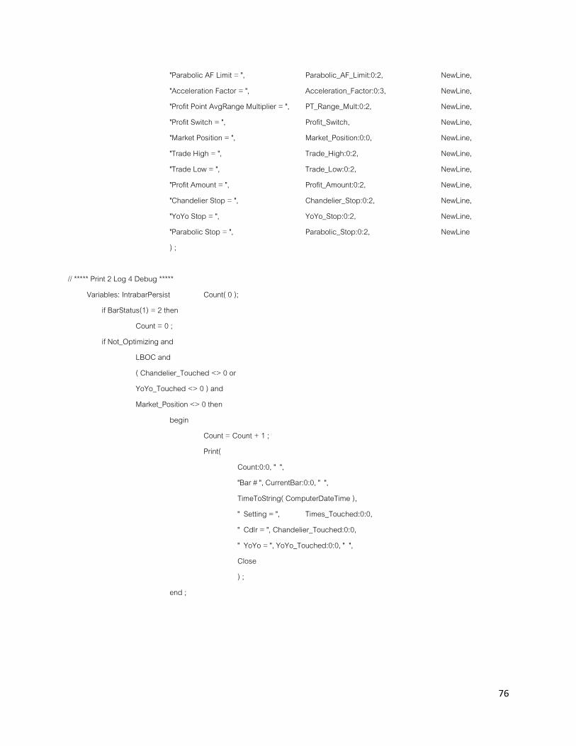
76

"Parabolic AF Limit = ", Parabolic_AF_Limit:0:2, NewLine, "Acceleration Factor = ", Acceleration_Factor:0:3, NewLine, "Profit Point AvgRange Multiplier = ", PT_Range_Mult:0:2, NewLine, "Profit Switch = ", Profit_Switch, NewLine, "Market Position = ", Market_Position:0:0, NewLine, "Trade High = ", Trade_High:0:2, NewLine, "Trade Low = ", Trade_Low:0:2, NewLine, "Profit Amount = ", Profit_Amount:0:2, NewLine, "Chandelier Stop = ", Chandelier_Stop:0:2, NewLine, "YoYo Stop = ", YoYo_Stop:0:2, NewLine, "Parabolic Stop = ", Parabolic_Stop:0:2, NewLine ) ;

// ***** Print 2 Log 4 Debug ***** Variables: IntrabarPersist Count( 0 );

if BarStatus(1) = 2 then Count = 0 ; if Not_Optimizing and LBOC and ( Chandelier_Touched <> 0 or YoYo_Touched <> 0 ) and Market_Position <> 0 then begin Count = Count + 1 ; Print( Count:0:0, " ", "Bar # ", CurrentBar:0:0, " ", TimeToString( ComputerDateTime ), " Setting = ", Times_Touched:0:0, " Cdlr = ", Chandelier_Touched:0:0, " YoYo = ", YoYo_Touched:0:0, " ", Close ) ; end ;

77

LeBeu Exit Short Code Input: slength(15), llength(15), vlength(15); If High > High[llength] and Close > Close[llength] and Volume > Volume[vlength] then buy next bar at market;

//***** Set-up *****

[IntrabarOrderGeneration = True] INPUTS: Chandelier_AvgRange (2.5), YoYo_AvgRange (2), Times_Touched (10), // MIT only if Chandelier and YoYo Parabolic_Accel_Factor (.01), // futures default -- for equities use 0.05 +- AvgRange_Length (21), Profit_AvgRange (1), Profit_Switch_Factor (0.6), Commentary_On ( False ) ;

VARIABLES: aChandelier_AvgRange( AbsValue( Chandelier_AvgRange ) ), //----------------------------------------------------| aYoYo_AvgRange ( AbsValue( YoYo_AvgRange ) ),

Parabolic_AF ( AbsValue( Parabolic_Accel_Factor ) ), // convert inputs to absolute value

aAvgRange_Length ( AbsValue( AvgRange_Length) ), aProfit_AvgRange ( AbsValue( Profit_AvgRange ) ),

Acceleration_Factor ( Parabolic_AF ), Parabolic_AF_Limit ( Parabolic_AF * 10 ), // set limit 10x factor Average_Range ( 0 ), Market_Position ( 0 ), IntrabarPersist Trade_High ( 0 ), // highest high of current trade IntrabarPersist Trade_Low ( 0 ), // lowest low of current trade YoYo_Amount ( 0 ), // YoYo stop amount YoYo_Price ( 0 ), // pin price to last bar close IntrabarPersist Chandelier_Stop ( 0 ), IntrabarPersist YoYo_Stop ( 0 ), // stop prices Parabolic_Stop ( 0 ), Profit_Amount ( 0 ), IntrabarPersist Profit_Switch ( False ), // point at which Chandalier Stop tightens Not_Optimizing ( True ),

78

GV_Name ( NumToStr( AbsValue( GetAppInfo( aiAppID ) ), 0 ) ), PT_On ( False ), // get from PT_MIT strategy IntrabarPersist Chandelier_Touched ( 0 ), IntrabarPersist YoYo_Touched ( 0 ), IntrabarPersist Bar_Number ( 0 ), PT_Range_Mult ( aProfit_AvgRange ), PT_Range_Length ( aAvgRange_Length ), PT_Average_Range ( 0 ), Avg_Entry_Price ( 0 ), aProfit_Switch_Fac ( AbsValue( Profit_Switch_Factor ) ), New_Entry ( False ) ;

//***** Housekeeping ***** if CurrentBar = 1 then

Not_Optimizing = GetAppInfo( aiOptimizing ) <> 1 ; //---------------------------------------------------------------------------------------------------------------------------------------| // This code gets the PT_MIT strategy settings to calculate the PT settings of the LeBeau | // Stops. If no PT_MIT present, then uses local LeBeau settings. | //---------------------------------------------------------------------------------------------------------------------------------------| if CurrentBar = 2 then

begin PT_Range_Mult = GVGetNamedDouble( GV_Name + "PT_Range_Mult", aProfit_AvgRange ) ; PT_Range_Length = GVGetNamedDouble( GV_Name + "PT_Range_Length", aAvgRange_Length ) ; if Not_Optimizing then begin Value1 = GVSetNamedDouble( GV_Name + "Chandelier_AvgRange", aChandelier_AvgRange ) ; Value2 = GVSetNamedDouble( GV_Name + "YoYo_AvgRange", aYoYo_AvgRange ) ; Value3 = GVSetNamedDouble( GV_Name + "Parabolic_AF", Parabolic_AF ) ; Value4 = GVSetNamedDouble( GV_Name + "LeBeau_AvgRange_Length", aAvgRange_Length ) ;

Value6 = GVSetNamedDouble( GV_Name + "Parabolic_AF_Limit",Parabolic_AF_Limit ) ; Value5 = GVSetNamedDouble( GV_Name + "Profit_AvgRange", PT_Range_Mult ) ; Value7 = GVSetNamedDouble( GV_Name + "LePT_Range_Length", PT_Range_length ) ; Value8 = GVSetNamedDouble( GV_Name + "Profit_Switch_Factor", aProfit_Switch_Fac ) ; end ; // not optimizing end ; // 2nd bar housekeeping

//***** Compute Stops *****

Market_Position = MarketPosition ; // in order to access historical bar market position

79

if BarStatus(1) = 2 then // calc only once per bar begin Average_Range = AvgRange( aAvgRange_Length ) ; Avg_Entry_Price = AvgEntryPrice ; New_Entry = Avg_Entry_Price[1] <> Avg_Entry_Price ; PT_Average_Range = AvgRange( PT_Range_Length ) ; Profit_Amount = Round( PT_Range_Mult * PT_Average_Range, 2 ) ; YoYo_Amount = aYoYo_AvgRange * Average_Range ; end // calc once else if Bar_Number <> CurrentBar then // calc on first tick of new bar formation begin Bar_Number = CurrentBar ; if Not_Optimizing and GetAppInfo( aiRealTimeCalc ) = 1 then begin Chandelier_Touched = 0 ; YoYo_Touched = 0 ; end // reset at end of bar if not optimizing else begin Chandelier_Touched = Times_Touched ; YoYo_Touched = Times_Touched ; end ; // if optimizing, set to limit end ; // reset touched each new bar if Market_Position[1] <> 0 then YoYo_Price = Close[1] else YoYo_Price = Open ; if Market_Position <> 0 then // eval market position on current bar begin

//*** Long Position *** if Market_Position = 1 then begin if Market_Position[1] <> 1 or New_Entry then // eval market position on prior bar and reset

variables if begin Profit_Switch = False ; // reset profit switch

80

Trade_High = High ; // reset trade high end // reset else if High > Trade_High then // find new high Trade_High = High ;

//* Chandelier Stop * if Profit_Switch or // if switch = true Trade_High >= AvgEntryPrice + ( Profit_Amount * aProfit_Switch_Fac ) then begin Profit_Switch = True ; Chandelier_Stop = Round( Trade_High - ( aChandelier_AvgRange *

Average_Range * aProfit_Switch_Fac ), 2 ) ; // tighten stop end // tighten Chandelier stop

when profit point exceeded else Chandelier_Stop = Round( Trade_High - ( aChandelier_AvgRange * Average_Range ), 2 ) ;

// normal stop if Market_Position[1] = 1 and New_Entry = False and Chandelier_Stop < Chandelier_Stop[1] then

Chandelier_Stop = Chandelier_Stop[1] ; // prevent retracement if Close <= Chandelier_Stop then Chandelier_Touched = Chandelier_Touched + 1 ;

//* YoYo Stop *

YoYo_Stop = Round( YoYo_Price - YoYo_Amount, 2 ) ; if Close <= YoYo_Stop then YoYo_Touched = YoYo_Touched + 1 ;

//* Parabolic Stop * if Market_Position[1] <> 1 or New_Entry then begin Parabolic_Stop = Chandelier_Stop ; // initial setting Round( AvgEntryPrice - ( aChandelier_AvgRange *

Average_Range ), 2 ) ; // tie to entry price Acceleration_Factor = Parabolic_AF ; end // eval market postion on prior

bar

81

else begin {if BarStatus(1) = 2 then begin} if Trade_High > Trade_High[1] and Acceleration_Factor < Parabolic_AF_Limit then Acceleration_Factor =

Acceleration_Factor + MinList( Parabolic_AF, Parabolic_AF_Limit - Acceleration_Factor ) ; Parabolic_Stop = Parabolic_Stop + Acceleration_Factor * (

Trade_High - Parabolic_Stop ) ; if Parabolic_Stop > Low then // force stop <= low of last bar Parabolic_Stop = Low ; {end ;} // update only at end of bar end ; // long parabolic stop end // long market postion

//*** Short Position *** else begin // short market position if Market_Position[1] <> -1 or New_Entry then // eval market position on prior bar begin Profit_Switch = False ; // reset profit switch Trade_Low = Low ; // reset trade low end else if Low < Trade_Low then // find new low Trade_Low = Low ;

//* Chandelier Stop * if Profit_Switch or // if switch = true Trade_Low <= AvgEntryPrice - ( Profit_Amount * aProfit_Switch_Fac ) then begin Profit_Switch = True ; Chandelier_Stop = Round( Trade_Low + ( aChandelier_AvgRange *

Average_Range * aProfit_Switch_Fac ), 2 ) ; // tighten stop end // tighten Chandelier stop when profit

point exceeded else Chandelier_Stop = Round( Trade_Low + ( aChandelier_AvgRange * Average_Range ), 2 ) ;

// normal stop if Market_Position[1] = -1 and

82

New_Entry = False and Chandelier_Stop > Chandelier_Stop[1] then Chandelier_Stop = Chandelier_Stop[1] ; // prevent retracement if Close >= Chandelier_Stop then Chandelier_Touched = Chandelier_Touched + 1 ;

//* YoYo Stop *

YoYo_Stop = Round( YoYo_Price + YoYo_Amount, 2 ) ; if Close >= YoYo_Stop then YoYo_Touched = YoYo_Touched + 1 ;

//* Parabolic Stop *

if Market_Position[1] <> -1 or New_Entry then begin Parabolic_Stop = Chandelier_Stop ; Round( AvgEntryPrice + ( aChandelier_AvgRange * Average_Range ),

2 ) ; // tie to entry price Acceleration_Factor = Parabolic_AF ; end // eval market postion on prior bar else begin {if BarStatus(1) = 2 then begin} Parabolic_Stop = Parabolic_Stop + Acceleration_Factor * ( Trade_Low

- Parabolic_Stop ) ; if Trade_Low < Trade_Low[1] and Acceleration_Factor < Parabolic_AF_Limit then Acceleration_Factor = Acceleration_Factor +

MinList( Parabolic_AF, Parabolic_AF_Limit - Acceleration_Factor ) ; if Parabolic_Stop < High[1] then Parabolic_Stop = High[1] ; {end ;} // only once per bar end ; // short parabolic stop end ; // short market position

//***** Exits ***** if Market_Position = 1 then begin

83

if Chandelier_Touched >= Times_Touched then Sellshort ( "LX_Cdlr" ) currentshares shares next bar at Chandelier_Stop STOP ; if YoYo_Touched >= Times_Touched then Sellshort( "LX_YoYo" ) currentshares shares next bar at YoYo_Stop STOP ; Sellshort ( "LX_Pblc" ) currentshares shares next bar at Parabolic_Stop STOP ; end // long stops else begin if Chandelier_Touched >= Times_Touched then BuyToCover ( "SX¯Cdlr" ) currentshares shares next bar at Chandelier_Stop STOP ; if YoYo_Touched >= Times_Touched then BuyToCover ( "SX¯YoYo" ) currentshares shares next bar at YoYo_Stop STOP ; BuyToCover ( "SX¯Pblc" ) currentshares shares next bar at Parabolic_Stop STOP ; end ; // short stops

end ; // set stops -- MarketPostion <> 0

//***** Commentary ***** if Commentary_On and

AtCommentaryBar then Commentary( ( Date - ( Year( Date ) * 10000 ) ):0:0, Time:5:0, " -- BarNumber = ", CurrentBar:5:0, NewLine, "High = ", High, NewLine, "Low = ", Low, NewLine, "Open = ", Open, NewLine, "Close = ", Close, NewLine, "PT_On = ", PT_On, NewLine, "AvgRange Length = ", aAvgRange_Length:0:0, NewLine, "AvgRange = ", Average_Range:0:2, NewLine, "Chandelier AvgRange Multip lier = ", aChandelier_AvgRange:0:2, NewLine, "YoYo AvgRange Multiplier =", aYoYo_AvgRange:0:2, NewLine, "Times Touched = ", Times_Touched:0:2, NewLine, "Parabolic Acceleration Factor = ", Parabolic_AF:0:3, NewLine, "Parabolic AF Limit = ", Parabolic_AF_Limit:0:2, NewLine, "Acceleration Factor = ", Acceleration_Factor:0:3, NewLine, "Profit Point AvgRange Multiplier = ", PT_Range_Mult:0:2, NewLine, "Profit Switch = ", Profit_Switch, Newline, "Market Position = ", Market_Position:0:0, NewLine, "Trade High = ", Trade_High:0:2, NewLine,

84

"Trade Low = ", Trade_Low:0:2, NewLine, "Profit Amount = ", Profit_Amount:0:2, NewLine, "Chandelier Stop = ", Chandelier_Stop:0:2, NewLine, "YoYo Stop = ", YoYo_Stop:0:2, NewLine, "Parabolic Stop = ", Parabolic_Stop:0:2, NewLine ) ;

// ***** Print 2 Log 4 Debug ***** Variables: IntrabarPersist Count( 0 );

if BarStatus(1) = 2 then Count = 0 ; if Not_Optimizing and LBOC and ( Chandelier_Touched <> 0 or YoYo_Touched <> 0 ) and Market_Position <> 0 then begin Count = Count + 1 ; Print( Count:0:0, " ", "Bar # ", CurrentBar:0:0, " ", TimeToString( ComputerDateTime ), " Setting = ", Times_Touched:0:0, " Cdlr = ", Chandelier_Touched:0:0, " YoYo = ", YoYo_Touched:0:0, " ", Close ) ; end ;

_Expectancy Function: Function: _Expectancy Description: Calculate annualized Expectancy (oExpectancy) and Expectancy per trade (oExpectPerTrade) popularized by Van K. Tharp and used to assess strategy performance. Author: Modification of function "Tharp" from Hook and _SystemQuality function from Alex Matulich (2/1/04) of Unicorn Research Corp Methodology proposed by Van K. Tharp and discussed in "Trade Your Way To Financial Freedom"

85

Recoded by MarkSanDiego. Updated: 09/09/09 initial revision 09/16/09 DoCalc variable removed. Original function created as series function in error. As a simple function, the DoCalc variable is unecessary. Usage: vars: int TradingDays(0), float oExpectPerTrade(0), float oExpectancy(0); { within calling strategy } if Date <> Date[1] then TradingDays = TradingDays + 1; if LastBarOnChart then begin value1 = _Expectancy(TradingDays, oExpectPerTrade, oExpectancy); end; } inputs: int TradingDays(NumericRef), { strategy trading days used to annualize the expectancy score } { outputs } float oExpectPerTrade(NumericRef), { expectancy per trade } float oExpectancy(NumericRef); { expectancy score annualized = expectancy * opportunities per year } vars: float TradesPerYear(0), { annualized trading opportunities in a year by multiplying TotalTrades by: trading days per year (252) / strategy trading days OR calendar days in year (365) / strategy calendar days } float AW(0), { average winning trade } float PW(0), { probability of winning trade ( total wins / opportunities ) } float AL(0), { average lossing trade } float PL(0); { probability of losing trade ( total losses / opportunities ) }

86

AW = iff( NumWinTrades > 0, GrossProfit / NumWinTrades, 0); AL = iff( NumLosTrades > 0, GrossLoss / NumLosTrades, 0); if TotalTrades > 0 then begin PW = NumWinTrades / TotalTrades; PL = NumLosTrades / TotalTrades; end else begin PW = 0; PL = 0; end; oExpectPerTrade = iff(AL = 0, AW * PW, -(AW * PW + AL * PL) / AL); { annualize results by calculating number of trades occuring per year } { There are 252 trading days per year. MaxList ensures a partial trading day is counted as at least 1 trading day } TradesPerYear = TotalTrades * 252 / MaxList(TradingDays, 1); { annualize expectancy } oExpectancy = oExpectPerTrade * TradesPerYear; _Expectancy = oExpectancy;

_Expectancy Code: Input: slength(15), Llength(15),VElength(15),VXlength(15); vars: int TradingDays(0), float oExpectPerTrade(0), float oExpectancy(0); //buy if High > High[Llength] and Close > Close[Llength] and Volume > Volume[VElength] then buy next bar at market; //sell if Low < Low[Slength] and Close < Close[Slength] and Volume > Volume[VXlength] then sell short next bar at market; { within calling strategy } if Date <> Date[1] then TradingDays = TradingDays + 1;

87

if LastBarOnChart then begin value1 = _Expectancy(TradingDays, oExpectPerTrade, oExpectancy); end; Print("ExpectancyPerTrade: ", oExpectPerTrade, " Expectancy: ", oExpectancy);

88

Section B: First Strategy (2004-2008)

Sample of Strategy Overlay on Stock Chart

APWR

CLMT

JST

89

KGS

NEU

NGLS

90

NRGP

NXG

91

Performance Summaries

APWR

92

CLMT

93

JST

94

KGS

95

NEU

96

NGLS

97

NRGP

98

NXG

99

Equity Curves

APWR

CLMT

100

JST

KGS

101

NEU

NGLS

102

NRGP

NXG

103

Trade Efficiency Graphs

APWR

CLMT

104

JST

KGS

105

NEU

NGLS

106

NRGP

NXG

107

Periodic Returns

APWR

CLMT

108

JST

KGS

109

NEU

NGLS

110

NGRP

NXG

111

Section C: Volume Entry (2004-2008)


APWR

CLMT

112

JST

KGS

NEU

113

NGLS

NRGP

NXG

114


APWR

115

CLMT

116

JST

117

KGS

118

NEU

119

NGLS

120

NRGP

121

NXG

122

Equity Curves

APWR

CLMT

123

JST

KGS

124

NEU

NGLS

125

NRGP

NXG

126


APWR

CLMT

127

JST

KGS

128

NEU

NGLS

129

NRGP

NXG

130

Periodic Returns

APWR

CLMT

131

JST

KGS

132

NEU

NGLS

133

NRGP

NXG

134

Section D: Volume Entry (2004-2008)


APWR

CLMT

135

JST

KGS

NEU

136

NGLS

NRGP

NXG

137


APWR

138

CLMT

139

JST

140

KGS

141

NEU

142

NGLS

143

NRGP

144

NXG

145

Equity Curves

APWR

CLMT

146

JST

KGS

147

NEU

NGLS

148

NRGP

NXG

149


APWR

CLMT

150

JST

KGS

151

NEU

NGLS

152

NRGP

NXG

153

Periodical Returns

APWR

CLMT

154

JST

KGS

155

NEU

NGLS

156

NRGP

NXG

157

Section E: Volume Entry (2007-2009)


APWR

CLMT

158

JST

KGS

NEU

159

NGLS

NRGP

NXG

160


APWR

161

CLMT

162

JST

163

KGS

164

NEU

165

NGLS

166

NRGP

167

NXG

168

Equity Curves

APWR

CLMT

169

JST

KGS

170

NEU

NGLS

171

NRGP

NXG

172


APWR

CLMT

173

JST

KGS

174

NEU

NGLS

175

NRGP

NXG

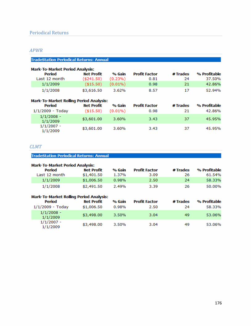
176

Periodical Returns

APWR

CLMT

177

JST

KGS

178

NEU

NGLS

179

NRGP

NXG

180

Section F: Volume Entry 2004-2009


APWR

CLMT

181

JST

KGS

NEU

182

NGLS

NRGP

NXG

183


APWR

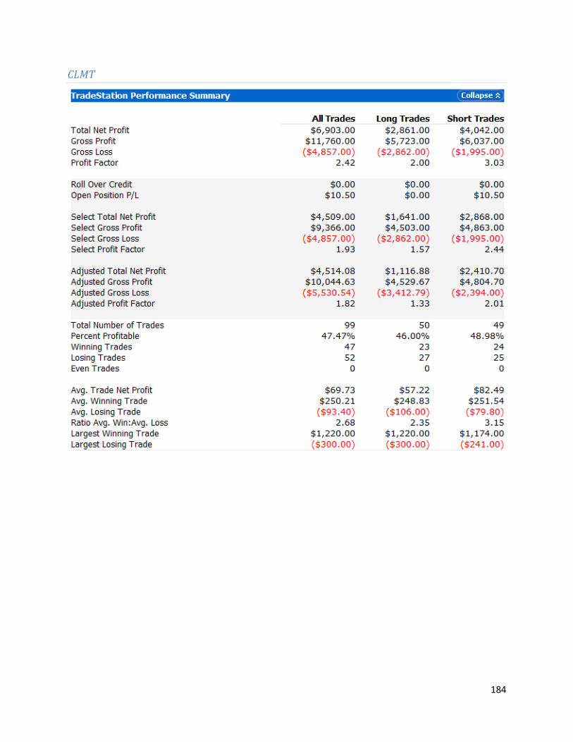
184

CLMT

185

JST

186

KGS

187

NEU

188

NGLS

189

NRGP

190

NXG

191

Equity Curves

APWR

CLMT

192

JST

KGS

193

NEU

NGLS

194

NRGP

NXG

195


APWR

CLMT

196

JST

KGS

197

NEU

NGLS

198

NRGP

NXG

199

Periodical Returns

APWR

CLMT

200

JST

KGS

201

NEU

NGLS

202

NRGP

NXG

203

Section G: LeBeau Exit 2004-2008


APWR

CLMT

204

JST

KGS

NEU

205

NGLS

NRGP

NXG

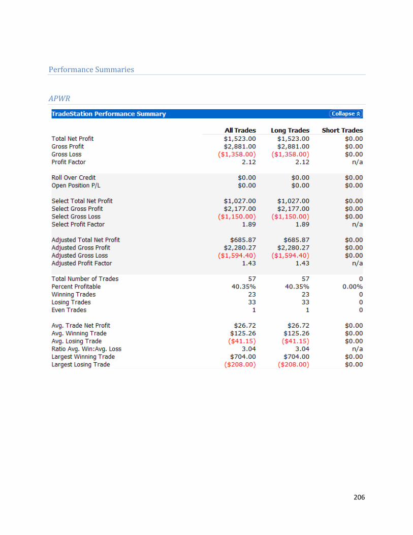
206


APWR

207

CLMT

208

JST

209

KGS

210

NEU

211

NGLS

212

NRGP

213

NXG

214

Equity Curves

APWR

CLMT

215

JST

KGS

216

NEU

NGLS

217

NRGP

NXG

218


APWR

CLMT

219

JST

KGS

220

NEU

NGLS

221

NRGP

NXG

222

Periodical Returns

APWR

CLMT

223

JST

KGS

224

NEU

NGLS

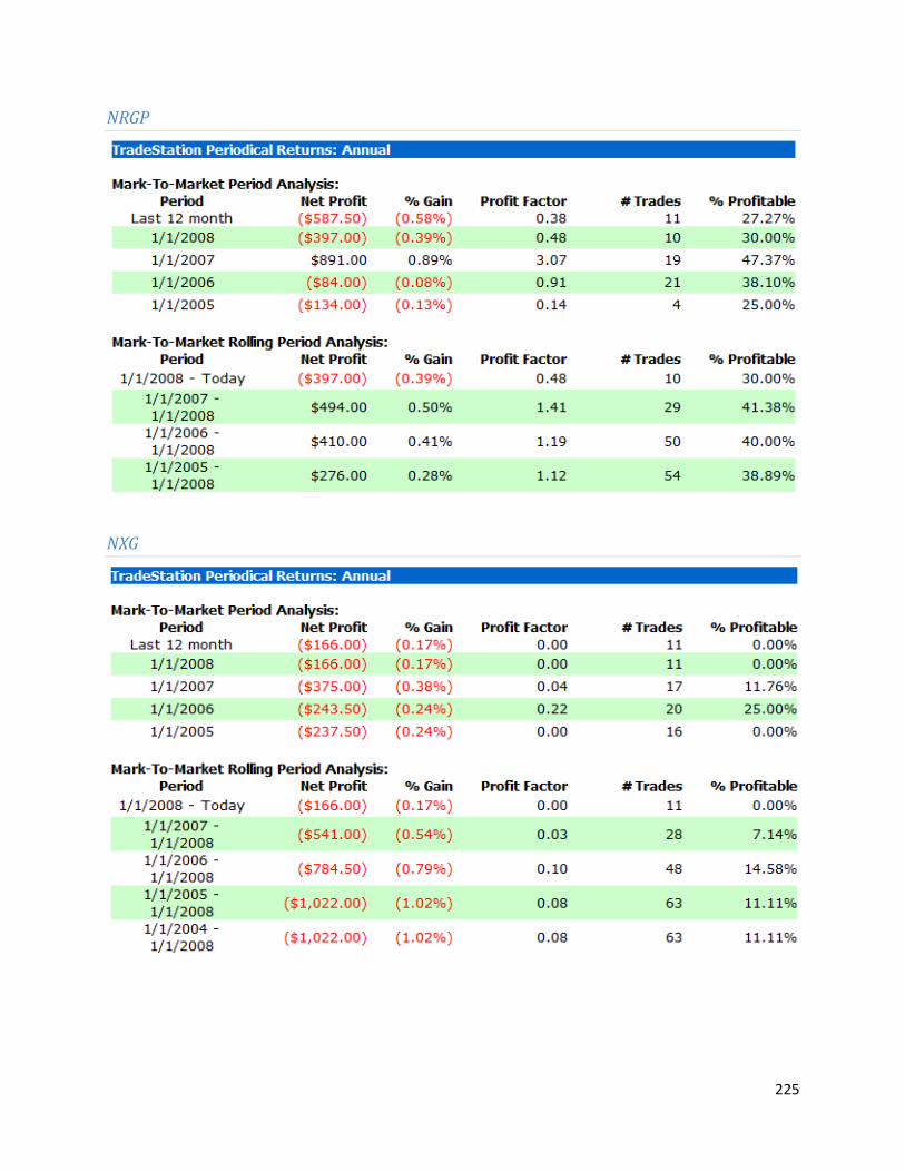
225

NRGP

NXG

226

Section H: LeBeau Exit (2007-2009)


APWR

CLMT

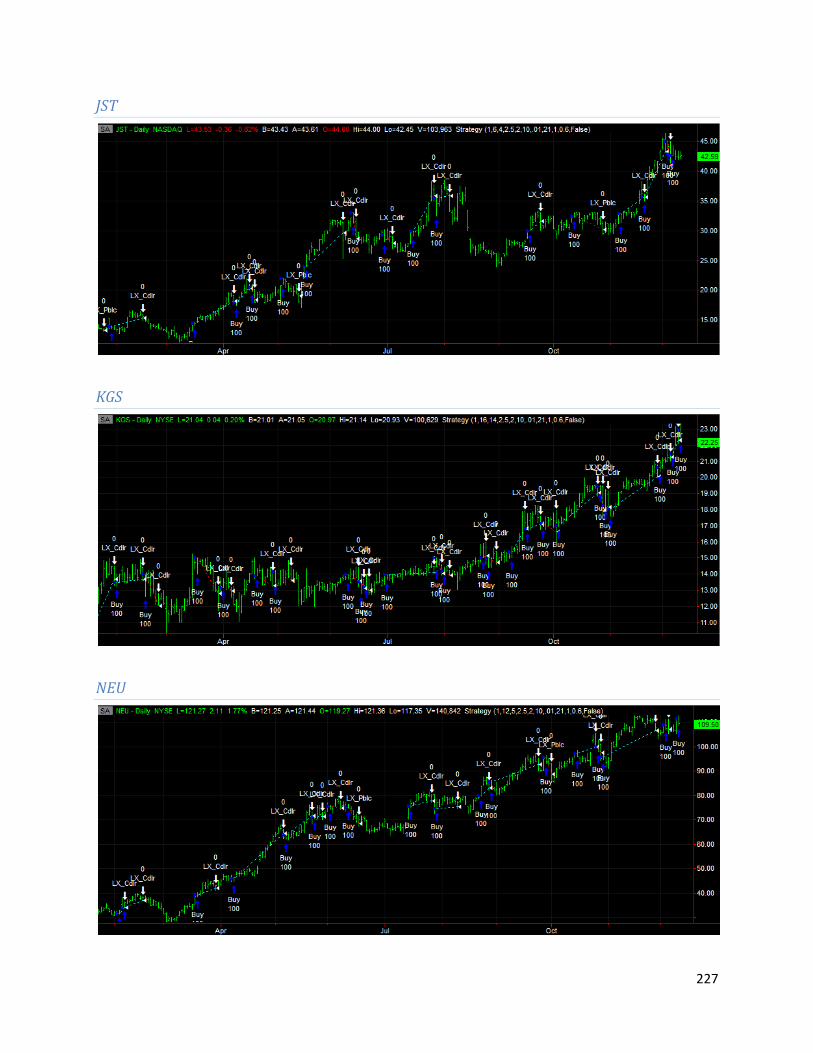
227

JST

KGS

NEU

228

NGLS

NRGP

NXG

229


APWR

230

CLMT

231

JST

232

KGS

233

NEU

234

NGLS

235

NRGP

236

NXG

237

Equity Curves

APWR

CLMT

238

JST

KGS

239

NEU

NGLS

240

NRGP

NXG

241


APWR

CLMT

242

JST

KGS

243

NEU

NGLS

244

NRGP

NXG

245

Periodical Returns

APWR

CLMT

vvv

246

JST

KGS

NEU

247

NGLS

NRGP

NXG

248

Section I: LeBeau Exit Short (2004-2008)


APWR

CLMT

249

JST

KGS

NEU

250

NGLS

NRGP

NXG

251


APWR

252

CLMT

253

JST

254

KGS

255

NEU

256

NGLS

257

NRGP

258

NXG

259

Equity Curves

APWR

CLMT

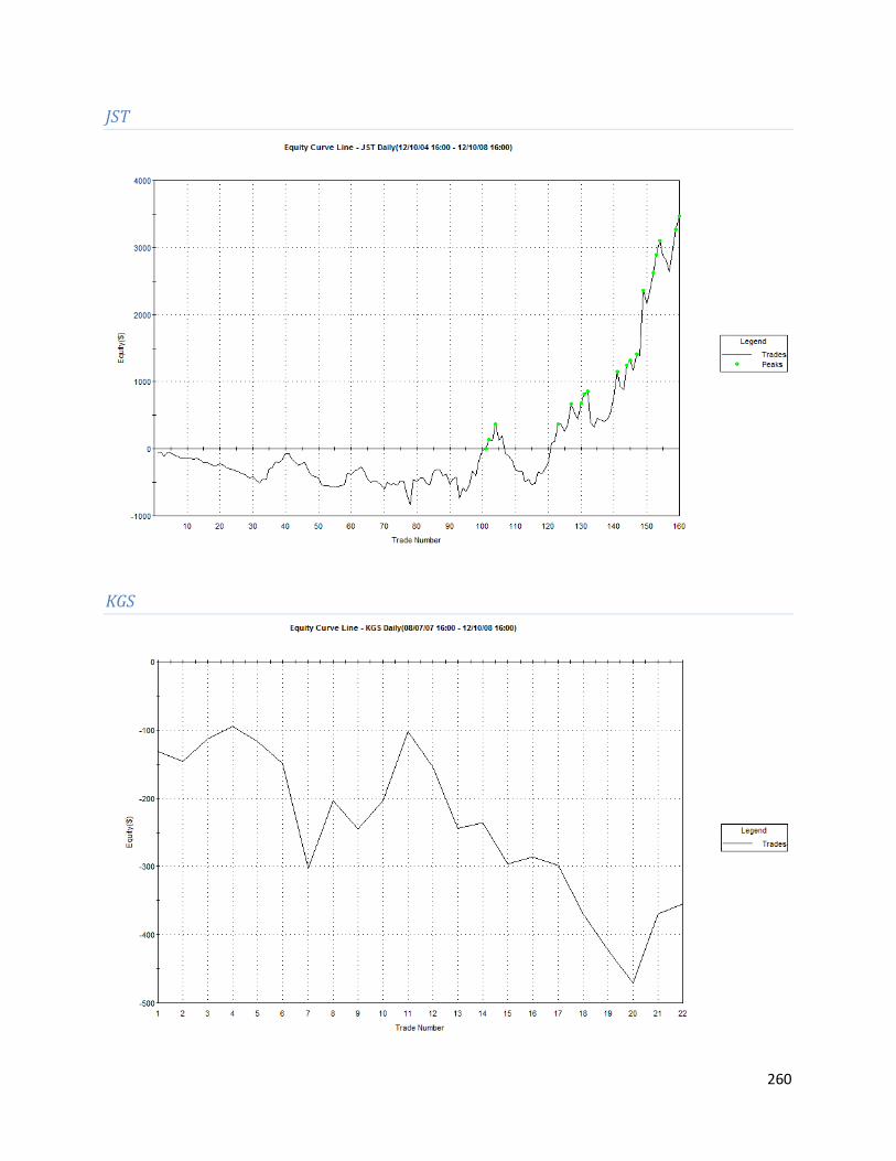
260

JST

KGS

261

NEU

NGLS

262

NRGP

NXG

263


APWR

CLMT

264

JST

KGS

265

NEU

NGLS

266

NRGP

NXG

267

Periodical Returns

APWR

CLMT

268

JST

KGS

269

NEU

NGLS

270

NRGP

NXG

271

Section J: LeBeau Exit Short (2007-2009)


APWR

CLMT

272

JST

KGS

NEU

273

NGLS

NRGP

NXG

274


APWR

275

CLMT

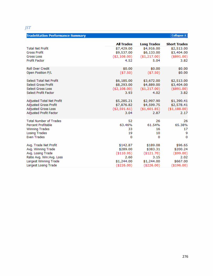
276

JST

277

KGS

278

NEU

279

NGLS

280

NRGP

281

NXG

282

Equity Curves

APWR

CLMT

283

JST

KGS

284

NEU

NGLS

285

NRGP

NXG

286


APWR

CLMT

287

JST

KGS

288

NEU

NGLS

289

NRGP

NXG

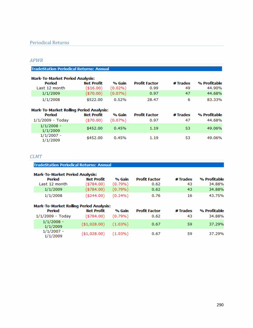
290

Periodical Returns

APWR

CLMT

291

JST

KGS

292

NEU

NGLS

NRGP

293

NXG

294

Section K: Communications with MarkSanDiego

Posted In: https://www.tradestation.com/Discussions/Topic.aspx?Topic_ID=93283&SearchTerm=expectancy&txtExactMatch= Posted - 12/30/2009 15:02:04 by WPITrader

"Mark, I am currently trying to use your code and noticed a discrepancy between the "usage"

sections on your forum post and that of the function code.

On your post you have the line "value1= _Expectancy(LastBar,...." where on your function code the

LastBar is omitted. When I try to verify the usage code, TradeStation says that "LastBar" is not

recognized, is this a separate function in addition to the _Expectancy function?

Thank you"

Posted - 12/30/2009 19:46:09 by MarkSanDiego

WPITrader,

The correct usage section is found in the comments section of the function itself:

vars: int TradingDays(0), float oExpectPerTrade(0), float oExpectancy(0); { within calling strategy } if Date <> Date[1] then TradingDays = TradingDays + 1; if LastBarOnChart then begin value1 = _Expectancy(TradingDays, oExpectPerTrade, oExpectancy);

end;

The usage example in the original post needs to be corrected. I will do so shortly. Thanks for pointing this

out.

Private Messages:

Sent - 01/01/2010 15:33:33

Expectancy Function

MarkSanDiego,

I am sorry to bother you again, but I appear to be having trouble with your Expectancy function again. I

am fairly new to TradeStation and the use of functions. I watched the TradeStation tutorial on functions

earlier today in hopes of learning how to view the output of a function. Within that tutorial they inserted

295

the function into an indicator which when plotted on the chart gave a graph of the value whereas the

Expectancy function gives a single value.

How does one go about viewing the output of the Expectancy Function? I have inserted the "usage"

section of your code into my strategy and loaded the _Expectancy function into TradeStation.

Thank you

-Erik Khzouz

Sent - 01/04/2010 03:21:32

RE: Expectancy Function

This function is called only from a strategy. You have to have a strategy that is making trades for it to

calculate a value. The last link in the post in the download section, shows sample code of how to call the

function from a strategy.

After you call this function from the strategy, you can use the Print function to output the result to the

EasyLanguage Output Bar, where you can see the result.

Mark

Sent - 01/04/2010 09:31:07


Thank you for your help, it makes a lot more sense now! The one piece of the puzzle that I was missing

before was the print function. Thank you again for your time!

-Erik

Sent - 01/04/2010 18:49:00


Mark,

I want to thank you again for your last response. After reviewing it as well as the "EasyLanguage Output

Techniques" tutorial I more clearly understand the use of the output bar and the print command.

I do appear to be running into one final snag though within my code using the print function.

Print("Date",Date,"Time",Time,"Expectancy",_Expect ancy);

The _Expectancy term is expecting an input to the function, should I be using oExpectancy here?

Also, am I correct in assuming copying the usage section of how to call the function from a strategy into

my strategy is correct? My current code is below:

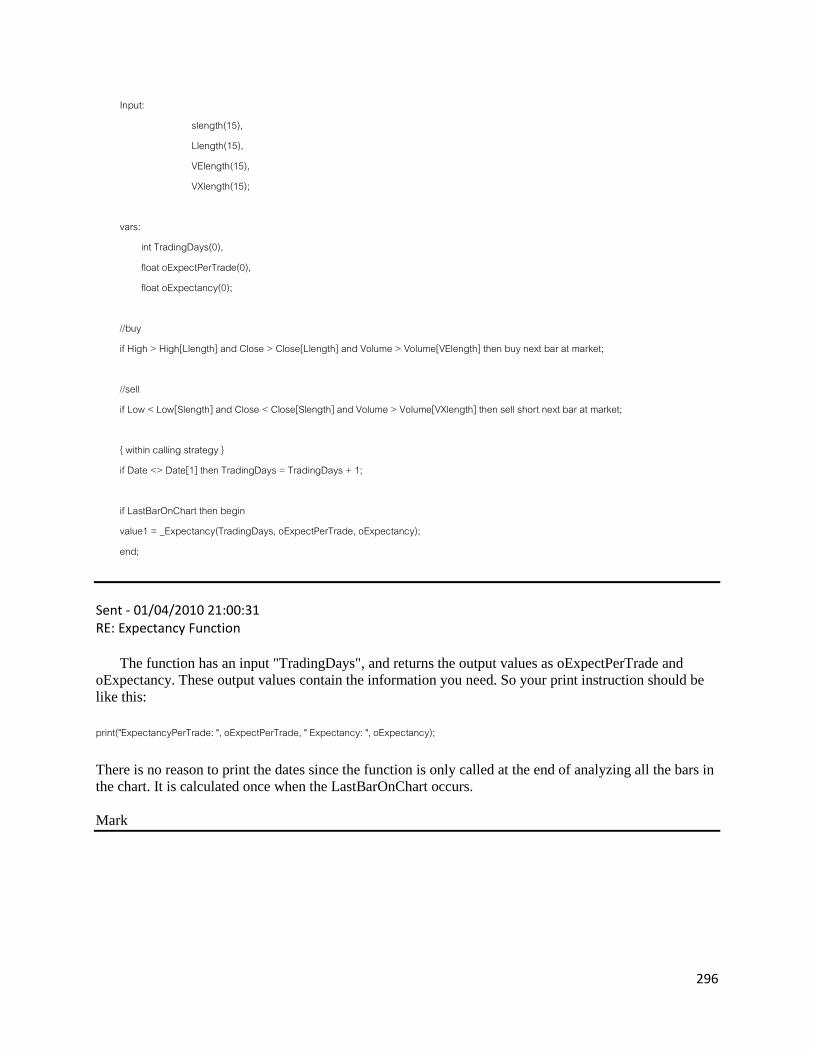
296

Input: slength(15), Llength(15), VElength(15), VXlength(15); vars: int TradingDays(0), float oExpectPerTrade(0), float oExpectancy(0); //buy if High > High[Llength] and Close > Close[Llength] and Volume > Volume[VElength] then buy next bar at market; //sell if Low < Low[Slength] and Close < Close[Slength] and Volume > Volume[VXlength] then sell short next bar at market; { within calling strategy } if Date <> Date[1] then TradingDays = TradingDays + 1; if LastBarOnChart then begin value1 = _Expectancy(TradingDays, oExpectPerTrade, oExpectancy); end;

Sent - 01/04/2010 21:00:31 RE: Expectancy Function

The function has an input "TradingDays", and returns the output values as oExpectPerTrade and

oExpectancy. These output values contain the information you need. So your print instruction should be

like this: print("ExpectancyPerTrade: ", oExpectPerTrade, " Expectancy: ", oExpectancy); There is no reason to print the dates since the function is only called at the end of analyzing all the bars in

the chart. It is calculated once when the LastBarOnChart occurs.

Mark

297

Sent - 01/06/2010 13:56:48


Mark,

I wanted to thank you again for your help over the past few days. I was able to get the desired output for

my strategy thanks to you. I would not have been able to figure it out without your support.

Thank you again,

-Erik

298

Bibliography

1. "American Association of Individual Investors." Unbiased Stock Investing & Personal Finance Education from a Nonprofit Source. 2010. AAII, Web. 5 Mar 2010. http://aaii.com/ 2. Krisburg, Mark J. "Van K. Tharp's Expectancy Function." TradeStation Forum. 11 Sep 2009. TradeStation Securities, Web. 5 Mar 2010. https://www.tradestation.com/Discussions/Topic.aspx?Topic_ID=93283&SearchTerm=expectancy&txtExactMatch= 3. LeBeau, Charles. "Chuck LeBeau's Trader Club." 2010. Charles LeBeau, Web. 5 Mar 2010. <http://www.traderclub.com/>. 4. Tharp, Van K. "Being Right and Making Money are Not Equivilant." Trader's Journal May 2005: 23-25. Web. 5 Mar 2010. http://www.mtptrader.com/TJMay.pdf 5. Wright, Charlie. "Trading as a Business." Elite Trader. 2010. Elite Trader, Web. 5 Mar 2010. http://www.elitetrader.com/tr/index.cfm

project number: salvador antoniou crn: 21493 erik … · 2010-03-05 · degree of bachelor of...

Documents