project appraisal guidelines - railway procurement · pdf fileproject appraisal guidelines...
TRANSCRIPT
July 2011
Unit 6.2 Guidance on using COBAProject Appraisal Guidelines
Project Appraisal Guidelines Unit 6.2
Guidance on Using COBA
Version Date Comments
1.0 July 2011 New Guidance
This document is available to download at www.nra.ie/publications/projectappraisal
For further queries please contact:
Strategic Planning Unit
National Roads Authority
St Martin’s House
Waterloo Road
Dublin 4
Tel: (01) 660-2511
Email: [email protected]
Web: www.nra.ie
NRA Project Appraisal Guidelines Unit 6.2: Guidance on Using COBA
Page | 1
1 Introduction
1.1. This PAG Unit provides information on the processes required to undertake a COBA
assessment. It deals with data collection, the inputs from the traffic model, and the
parameter values that should be used for assessments at the different phases of a
road scheme.
1.2. This PAG Unit also addresses the structure of the COBA input and how the data file
may be prepared and edited for input to the COBA programme.
1.3. After completion of a COBA assessment, it is necessary to submit a full report to the
National Roads Authority (NRA), the content of which is outlined in PAG Unit 6.12:
CBA Report. The steps to be undertaken in completing an audit of the COBA print
out and the requirements for Handover, Review & Closeout are also explained in
PAG Unit 6.12: CBA Report.
1.4. A specific version of the COBA software has been developed by Transport Research
Laboratory (TRL) for use on road schemes in the Republic of Ireland. A report
prepared by the TRL documenting the development of the Irish COBA is included as
PAG Unit 6.3: TRL COBA Report.

NRA Project Appraisal Guidelines Unit 6.2: Guidance on Using COBA
Page | 2
2 Data Requirements
General
2.1. COBA has the flexibility for a number of input parameters to be modified by the user
to better reflect local conditions. However, the use of standard values and
relationships is central to the COBA concept and, at the early stages of scheme
assessment, this avoids the need for time consuming and costly data collection
exercises.
2.2. The decision to use local or national default values depends on the phase of the
scheme assessment. At Route Selection, local values may be used where available,
although national values are normally acceptable. However at Design Stage, local
data should be input where it is both reliable and significantly different from national
COBA values.
2.3. This Section sets out the different categories of data required, how such data should
be compiled and whether local or national data are more appropriate for the CBA
process.
Data Categories
2.4. Data input into COBA can be classified into three categories, according to the
source, as illustrated in Table 6.2.1:
• Data that is always local;
• Data that should be local if values are reliable and differ significantly from
national values; and
• Data that should always be national.
Table 6.2.1: Summary of Data Required for COBA
Always Local Local or National Always National
Scheme costs Seasonality index Values of time
Link geometric characteristics E-Factor Accident costs
Junction geometric
characteristics M-Factor Economic growth
Link flows Traffic mix proportions Vehicle operating cost
parameters
Junction turning proportions Flow groups Taxation
Accident rates and
casualty proportions Traffic growth profiles
Speed-flow curves Discount Rate
Vehicle occupancy Consumer Price Index

NRA Project Appraisal Guidelines Unit 6.2: Guidance on Using COBA
Page | 3
Relative Price Factor
Carbon Costs
2.5. The data input can, in essence, be grouped under six key headings as follows:
• Scheme costs;
• Link geometry;
• Junction data;
• Traffic data;
• Accident data; and
• Economic values.
Scheme Costs
2.6. The scheme cost is made up from the following elements:
• Construction costs;
• Land and property costs;
• Preparation costs (planning and design);
• Supervision costs; and
• Maintenance costs.
2.7. Scheme costs can be entered into COBA using two different input keys
• KEY054 – user inputs Construction and Land Cost estimates and COBA calculates the equivalent costs in the present value year for construction, land, preparation and supervision and allocates them to the correct year; or
• KEY055 – allows the user to enter total scheme costs according to a
manually calculated profile of expenditure.
2.8. Both keys allow the user to specify the sector incurring the cost (i.e. Central or Local
Government) and any contributions from private developers.
2.9. In each case, costs are entered into COBA exclusive of indirect taxation, i.e. in the
factor cost unit of account. COBA uses indirect taxation rates held within the program
to convert factor costs into market prices.

NRA Project Appraisal Guidelines Unit 6.2: Guidance on Using COBA
Page | 4
2.10. Costs are entered into COBA as undiscounted values. COBA uses information on
the discount rate to derive discounted values.
2.11. KEY054 converts prices to the price base year using information provided by the
user on the Consumer Price Index at the base year and the year in which the
estimate was made. When using KEY055, costs are entered in price base year, i.e.
after taking into account the effects of inflation.
2.12. It is an NRA requirement that KEY055 is used to enter costs. Detailed guidance on
how to derive the profile of scheme costs for input into COBA KEY055 can be found
in PAG Unit 6.7: Preparation of Scheme Costs.
Link Geometry
2.13. The geometric characteristics for the links and junctions included in the COBA
network should be obtained from suitably scaled plans of the existing and proposed
road network. These characteristics are supported by field measurements of those
elements on the existing network that are to be included in the assessment.
2.14. The following data relating to links are required:
• Type of link – to allocate the speed-flow relationship, with links defined in
accordance with the classifications in Table 6.2.4 (see Section 4);
• Speed limit;
• Length;
• Width – including widths of any hard shoulders, hard strips and verges;
• Hilliness;
• Bendiness;
• Number of major junctions or accesses per kilometre;
• Degree of development fronting the link; and
• Sight distances.
2.15. The list above is an outline of the information necessary. The complete set of
information necessary for each link depends on the link type (e.g. rural, urban,
suburban, dual or single carriageway etc.). Full details of the data requirements,
including definitions and their derivation, are given in the UK DMRB Volume 13,
Section 1, Chapter 5.

NRA Project Appraisal Guidelines Unit 6.2: Guidance on Using COBA
Page | 5
Junction Data
2.16. For junctions that are to be modelled explicitly, the level of detail to be collected
depends on the type of junction; i.e. signal controlled, roundabout, signalised
roundabout, merge or priority junction that is being modelled. An indication of the
data requirements for each junction type is provided below:
• For all junction types, the junction will need to be defined as either rural or
urban and whether the entry arms are single or dual-carriageway;
• For priority junctions, the major and minor arms and any stagger should be
identified. The width of the carriageway for the various turning streams
should be measured along with the geometry of any central reserves and
sight distances;
• For roundabouts, the user must specify if the junction is grade separated or
not, and specify the geometry of the entry arms and of the circulatory
carriageway;
• For signal-controlled junctions, including signal-controlled roundabouts, the
user will need data on the staging arrangement at the junction along with the
geometry and gradient of the approach arms. Signal- controlled roundabouts
also require data on the saturation flows for each approach arm, and the data
for flared entry arms; and
• For merge junctions at grade-separated interchanges, the number of lanes
downstream from the merge is required.
2.17. Full details of the data requirements for junctions are given in DMRB Volume 13,
Section 1, Chapter 6.
2.18. Note that modelling junctions is not an explicit requirement in COBA models.
Guidance on the inclusion of junction modelling is included in Section 3 of this PAG
Unit.
Traffic Data
2.19. Traffic flow data, in the form of link flows and turning proportions are normally
obtained from a traffic model, the complexity and extent of which will reflect the
nature of the scheme. For further information on the development of traffic models,
see PAG Unit 5.2: Construction of Transport Models.
2.20. For the traffic count data, long-term data (i.e. over a period of at least one-year) are
required to establish local values for the following parameters:
• Seasonality index;
• E-factor;
• M-Factor; and
• Vehicle mix proportions.
2.21. Default values for these parameters, applicable to the assessment of road schemes,
and the derivation of scheme specific parameter values for the above parameters are
discussed in more detail in Section 4.

NRA Project Appraisal Guidelines Unit 6.2: Guidance on Using COBA
Page | 6
2.22. Journey time surveys allow validation of the base year COBA model by comparing
modelled journey times with actual recordings. They also provide data for locally
adjusting the maximum delay parameter at junctions.
Accident Data
2.23. Local data on the occurrence and severity of accidents should relate to a period
when the conditions on the road have been broadly unchanged (for example, no
abnormal changes in traffic flow, no changes in junction design or road geometry,
etc.). Local data should ideally cover the five years previous to the COBA
assessment but in all cases must cover a period of at least three years.
2.24. In addition, accident data should be checked to identify any particular anomalies
where it is suspected that they do not accurately reflect the accident history of the
link. Where such anomalies do exist, accident data may need to be processed or
adjusted before inputting to the COBA data file. One such example is where road
works led to a significant change in the accident rate over a period of one year during
a five year period. In such a case it may be appropriate to manually interpolate data
for that year, or to adopt default accident rates.
2.25. The number of accidents in each year is input, including zero for those links or years
where no accidents occurred, and COBA will then internally produce a local accident
rate (accidents per million vehicle kilometres) for each link.
2.26. If insufficient data are available to allow computation of local accident rates, then the
default national default values should be used.
2.27. Only those accidents recorded by the Gardaí will be manifest in accident data,
however the Gardaí are not always in attendance at the scene of accidents,
especially when no injuries occur. The COBA program assumes that only one third of
minor injury accidents and two thirds of serious injury accidents are reported, and
applies factors to observed data within the COBA program to account for this.
Economic Values
2.28. The COBA user must make use of the most recent data on economic parameter
values. Further information on the application of national parameter values is
provided in Section 18 of PAG Unit 6.1: Guidance on Conducting CBA. Values are
set out in PAG Unit 6.11: National Parameter Values Sheet.
2.29. National default values are applicable for all economic parameters regardless of the
scheme assessment phase. These values are contained within the COBA program
and must not be changed unless instructed to do so by the NRA.

NRA Project Appraisal Guidelines Unit 6.2: Guidance on Using COBA
Page | 7
3 Scoping a COBA Model
General
3.1. The COBA user is required to provide a description of the road network to cover both
the existing situation and the proposed improvements. The basis of this will be a
conventional traffic model, from which link flows for input into the COBA assessment
will be obtained. In this Section the structure of the COBA model and its interface
with a conventional traffic model is described. For more specific advice regarding
traffic modelling, PAG Unit 5.0: Transport Modelling should be consulted.
Extent of Network
3.2. The COBA network should extend far enough from the improvement to include all
links on which there is a substantial difference in the assigned traffic flows between
the Do-Minimum and Do-Something networks. If the scheme is expected to result in
a significant change in the flow level on a competing route, that route should be
included in the network. This concept should be balanced by the consideration that,
as the network spreads, benefits arising from the scheme in distant areas are
inherently less plausible and more difficult to assess than local benefits. It is
recommended that, as a general rule, the extent of the COBA network should be the
same as the assignment network, to avoid possible bias from the omission of links.
Even the smallest differences in the matrix of trips used on the assessment networks
can affect the results.
3.3. The assignment network and the COBA network therefore need to be compatible in
three respects:
(i) Detail of network;
(ii) Description of links and junctions; and
(iii) Incorporation of future changes to network.
Journey Time Information
3.4. The journey times from most traffic models will be inadequate for economic appraisal
using COBA, since they represent short period models that do not differentiate
between travel at different times and in different traffic conditions. For some
schemes, especially inter-urban ones, the flow group and speed-flow analysis
incorporated in COBA can be used to calculate journey times across different
periods. The facility in COBA to print out journey speeds and times for each flow
group in a specified year can be used to check that the two networks are broadly
compatible.
3.5. In areas where traffic congestion exists or will exist during the appraisal period, it is
important that the predictions of the traffic model are thoroughly validated. Methods
of determining the accuracy of journey times and the number of journey time runs
required to achieve a given level of accuracy are set out in Section 7 of this PAG
Unit.

NRA Project Appraisal Guidelines Unit 6.2: Guidance on Using COBA
Page | 8
Modelling Junctions
3.6. An accurate replication of existing journey times through the network can be difficult
if this relies on link transit times alone. In such cases, the inclusion of junctions will
allow a more accurate reflection of traffic behaviour. As such, the requirement to
model junctions in a COBA network will arise if the presence of junctions on the
existing road significantly impacts on journey time through the network
3.7. COBA models all junctions in isolation, with all arrivals assumed to be random; no
allowance is made for any junction interaction. Therefore, great care must be taken
when modelling junctions in the same area of the network where the capacity of one
junction controls the flow at another, either now or at some time in the future. If this
occurs it may only be necessary to model the controlling junction. Double counting
of delay must be avoided.
3.8. The concept of maximum delay has an important bearing on junction modelling in
COBA. The form of the COBA junction delay formulae implies that, as the capacity
of the junction is reached, delays increase very rapidly. However, COBA includes,
as default, a maximum delay at junctions of 300 seconds for peak flow group types.
3.9. If journey time evidence warrants a local adjustment for any individual junction, the
user may change the value for the peak group upwards or downwards (maximum
900 seconds). The maximum delay is attributed to all vehicles but on an arm-by-arm
or stream-by-stream basis. Maximum delays for the non-peak flow groups are
calculated as a proportion of the peak maximum delay, shown in Table 6.2.2.
Table 6.2.2: Maximum Delay by Flow Group
Accident Only and Delay Only Junctions
3.10. Delay-Only junctions are used to model user specified geometric delay at
roundabouts or points in the network where the speed flow relationships do not
apply. The specified delay is applied to all vehicle types and is constant over all flow
groups.
3.11. An Accident-Only node may be used to model accidents at a node without modelling
junction delays. This is important for urban junctions, where the delay is subsumed
into the link speed/flow relationships. As national accident data is only available on a
link and junction basis, Accident-Only nodes are not to be used without prior
approval of the NRA.
Flow Group Type Proportion of Maximum
Delay
Default Maximum Delay
(seconds)
Type 1 (off Peak) 0.4 120
Type 2 (Adjacent to Peak) 0.6 180
Type 4 (Peak) 1.0 300

NRA Project Appraisal Guidelines Unit 6.2: Guidance on Using COBA
Page | 9
2010
2009
JulyCPI
CPICostAvailableLatestpricesyearbaseaverageinCost ×=
4 National Parameter Values
4.1. COBA contains a series of default values for parameters relating to economic values
(for example, time, accidents, vehicle operating costs and carbon costs), accidents
(rates and severity), annual traffic flow patterns and vehicle composition (E and M-
factors and flow groups). These parameters have been developed specifically for
the assessment of road schemes in the Republic of Ireland.
4.2. This Section provides a general discussion on the various parameters, followed by a
more detailed discussion of the approach to selecting parameters at the different
phases of scheme development. All data is summarised in PAG Unit 6.11: National
Parameter Values Sheet.
Economic Parameters
4.3. The economic input parameters are fixed and do not change by project phase.
Some notes on these parameters are included below.
Key Parameters
4.4. The Present Value Year is that year for which costs and benefits are expressed. The
Present Value Year for the appraisal of road schemes should be 2009.
4.5. A discount rate of 4% shall be adopted; this is in line with latest Department of
Finance guidance. This rate should be applied across the 30 year appraisal period.
4.6. The Appraisal Period is the period over which costs and benefits are accounted. The
appraisal period shall be 30 years, although an allowance is made for the accrual of
additional costs and benefits after this period through the calculation of residual
value.
4.7. Consumer Price Indices (CPI) are used to adjust prices to the price base year. Up to
date information on the CPI can be obtained from the Central Statistics Office
website (http://www.cso.ie). For example, to adjust a price from July 2010 to the
present value year (for the purpose of this example, average 2009 prices) one would
apply the following formula:
4.8. The Relative Price Factor (RPF) describes that process which adjusts construction
costs to their long term average, effectively correcting for the sharp rise and fall of
construction prices that occurs through economic cycles. This process is separate
from adjustments based on the CPI. Current advice is for a value of unity to be
adopted for the RPF at all project phases.

NRA Project Appraisal Guidelines Unit 6.2: Guidance on Using COBA
Page | 10
2cVbVaC ++=
Maintenance Costs
4.9. Road maintenance costs have been developed for the following road classes:
• Standard 2-lane with hard shoulder;
• Wide 2-lane with hard shoulder;
• Type 3 Dual Carriageway (2+1);
• Type 2 Dual 2 Lane Carriageway; and
• Type 1, Standard and Wide Dual Carriageway/Motorway.
4.10. Maintenance costs are presented as a rate per kilometre per year. The maintenance
type relating to each road class is included in Table 6.2.4.
Value of Time
4.11. Forecast growth in real gross national product (GNP) per person employed has been
used to determine future changes in the real value of time. The same growth factor
is applied for work, commuting and other non-work time, although the facility exists to
use different factors.
Value of Accidents
4.12. Forecast growth in real GNP per person employed has also been used to determine
future changes in the real value of accidents. The assumption is that the values of
most elements of accident costs are proportional to national income.
Vehicle Operating Costs – Fuel
4.13. COBA calculates fuel costs using a function based on the average vehicle speed on
each link. The function includes a number of constants known as the a, b, and c
parameters. These vary by vehicle class to reproduce the different fuel operating
cost characteristics of different vehicle types.
4.14. The COBA vehicle operating cost formula is of the form:
where:
• C = cost in cents per kilometre per vehicle;
• V = average link speed in km/h, and
• a, b and c are vehicle category parameters.
4.15. The a, b and c parameters are contained in COBA both in cents/km and litres/km at
resource cost. Conversion between the two is simply a case of factoring the
parameters by the resource cost of fuel (cents per litre).

NRA Project Appraisal Guidelines Unit 6.2: Guidance on Using COBA
Page | 11
/Vb a C11
+=
Vehicle Operating Costs – Non-Fuel
4.16. Non-fuel vehicle operating costs include oil, tyres, maintenance and mileage. Only
items that vary with the use of the vehicle are measured and parameters are
presented by vehicle class. Non-fuel costs are calculated using the equation:
where:
• C= cost in cents per kilometre per vehicle;
• V= average link speed in km/h, and
• a1 and b1 are vehicle category parameters.
Value of Time Growth
4.17. In future years the real value of time will change as productivity increases. Factors
have been developed to take into account these changes such that they can be
accounted for through the appraisal period.
Value of Accident Growth
4.18. Factors are also derived to define the growth in the valuation of accidents. These
are deemed to be similar to value of time increases.
Vehicle Operating Cost Growth
4.19. Small changes are expected in fuel price and fuel consumption. No change in non-
fuel operating costs are expected.
Indirect Tax Rates
4.20. COBA requires inputs on average tax on final consumption, tax on fuel (final
consumption) and tax on fuel (intermediate consumption). This allows input costs to
be converted from resource costs to market costs, and hence allows an assessment
of the cost and benefit stream for different market segments.
Future Changes in Indirect Tax Rates
4.21. Any change in taxation levels is proposed by Government, and the implications of
such tax changes on various segments of society are considered independently from
the CBA process. The CBA should therefore assume that tax rates remain static
throughout the assessment period.
Emission Costs
4.22. The COBA program takes account of emissions of the following gases:
• Carbon Dioxide (CO2);

NRA Project Appraisal Guidelines Unit 6.2: Guidance on Using COBA
Page | 12
• Nitrous Oxide (N2O);
• Volatile Organic Compounds (VOC);
• Nitrogen Oxides (NOX); and
• Particulate Matter (PM), both urban and rural.
4.23. Emissions are considered in terms of the change in the equivalent tonnes released
as a result of implementing a road scheme. Emissions are estimated from fuel
consumption in the Do-Minimum and the Do-Something options. The change in
tonnes emitted and the monetary value given to the change is calculated in COBA.
4.24. Emissions costs (greenhouse and non-greenhouse gases) change with respect to
time and these changes are included within the COBA program. Current Department
of Finance guidance indicates that each tonne of CO2 equivalent should be costed at
€39 from 2015 onwards. This is based on expected value of carbon emanating from
the European Emissions Trading Scheme. However, over time as trading schemes
become more comprehensive, it is likely that the values emanating from them will
approach those arising from abatement costs and the value of €39 will be too low.
4.25. Based on the anticipated value of abatement costs in 2060 as determined by the UK
Department of Transport, the value of €39 per tonne would need to grow at a rate of
4 per cent per annum in real terms over the period to 2060 to reflect the rise in
abatement cost values. An adjustment factor or 4 per cent per annum should
therefore be applied to post 2015 values.
Traffic Input Parameters
Seasonality Index
4.26. The Seasonality Index is an important descriptor of annual traffic flow patterns. It is
defined as the ratio of the average August weekday (Monday to Friday) flow to the
average weekday flow in the neutral months of April, May, June, September and
October (excluding periods affected by bank holidays). Long-term automatic traffic
counter data is required to derive local values. A good estimate can be arrived at by
comparing the weekday traffic flows from a three-week continuous count in August
with one from late May/June or October.
E-Factor
4.27. The E-factor converts flows entered into the program as 12-hour values into the 16-
hour equivalent. Local relationships between the 12-hour and 16-hour flows can be
derived from long-term automatic traffic counts. It is preferable that AADT flows are
manually calculated from traffic model outputs using a relationship based on
observed local data representing a full year.

NRA Project Appraisal Guidelines Unit 6.2: Guidance on Using COBA
Page | 13
N
N AA β×=0
M-Factor
4.28. The M-factor converts flows entered into the program as 16-hour values into an
Annual All Vehicle Flow (AAVF). A local M-factor can be derived that relates the
average weekday 16-hour count in the month specified to the annual all vehicle flow.
Long-term automatic traffic counter data will be required to do this. It is preferable
that AADT flows are manually calculated from traffic model outputs using a
relationship based on observed local data representing a full year.
Link and Junction Combined Accident Rates and Casualty Proportions
4.29. COBA provides default data for the frequency, severity and the number of casualties
resulting from accidents associated with different road types.
4.30. If default accident values are to be replaced with local values, the COBA user must
demonstrate that the local severity split is significantly different in statistical terms
from the default national averages, and not a result of one or two particularly bad
accidents, the effect of which will be evened out by less extreme accidents as time
goes by. Adjustments are made automatically within the COBA program to account
for accident under-reporting. As a result, the number of minor accidents is
automatically multiplied by 3 and the number of serious accidents by 1.5.
4.31. Where no local data are available and for the Do-Something scheme components,
the default national parameter values should be used.
Accident Reduction Factors
4.32. COBA takes into account the existing long-term declining trend in accident rates and
severity. The program uses a ‘β-factor’ to model the reducing number of accidents in
each assessment year and also to model the reduction in the average number of
casualties, by severity split, resulting from each accident.
4.33. The change in accident rates and number of severities per accident is explained by
the relationship:
Where:
• AN = the accident rate or number of casualties per accident N years after
base year;
• A0 = the accident rate or number of casualties per accident in the base year;
and
• βN = change coefficient raised to the power N.
4.34. For the assessment of road schemes β-factors have been developed to take into
account Irish policy on the reduction of road traffic accidents. Default β-factors
contained within the COBA program are provided in PAG Unit 6.11: National
Parameter Value Sheet.

NRA Project Appraisal Guidelines Unit 6.2: Guidance on Using COBA
Page | 14
4.35. The β-factors are applied for any year between 1998 and 2016. Between 2017 and
2026, and between 2027 and 2036 the reduction factors are assumed to be one half
and one quarter respectively of the 1998 to 2016 reduction. For example, if the
coefficient β is 0.9, then it is 0.95 for the period 2017 to 2026 (or [1+β]/2), and 0.975
for the period 2027 to 2036. Zero change is assumed post 2036.
4.36. There is no facility to change how β varies with respect to time as this is embedded
within the COBA program.
Vehicle Category Proportions
4.37. Based on the flow groups in Table 6.2.5 default national values have been derived
for the vehicle category proportions in each of the flow groups, for each network
classification. Category proportions have also been derived for vehicles falling into
each of the three time modes.
AADT Adjustment Factors
4.38. Provided for conversion of 12-hour or 16-hour traffic flows to AADT. Note however
that it is preferable that AADT flows are manually calculated from traffic model
outputs using a relationship based on observed local data representing a full year.
Vehicle Category Correction Factors
4.39. Factors are provided for cases where flows are entered as 12-hour or 16-hour
counts. It is preferable that AADT flows are manually calculated from traffic model
outputs using a relationship based on observed local data representing a full year.
Vehicle Category Proportion Correction Factors
4.40. Correction factors were calculated using the formula
Vehicle proportion correction factor = Flow group proportion/annual proportion
4.41. Note that annual proportions are only determined for flow groups 2 to 4 and 7 to 9
and for vehicle types 2 and 5. Vehicle flows for cars and for flow groups 1 and 6 are
calculated within COBA by means of a balancing procedure. The results are shown
below.
Vehicle Occupancy
4.42. National default values for the average number of people occupying a vehicle of a
given category and time mode (work, commuting and other) have been developed
from roadside interview data.
4.43. The default values also give occupancy rates for three of the eight flow groups,
described in Table 6.2.5; i.e. Flow Groups 2, 3 and 4. For Flow Group 1, which
relates to the overnight off-peak traffic, and Flow Groups 6 – 9, which relate to
weekend traffic, the UK default value has been taken (adjusted to account for the
NRA Project Appraisal Guidelines Unit 6.2: Guidance on Using COBA
Page | 15
average occupancy of working cars in Flow Groups 2 – 4), since the source roadside
interview data only covered the 12-hour period from 07:00 to 18:45.
Vehicle Proportions by Time Mode and Flow Group
4.44. Default values are provided for the allocation of AADT to the various flow groups.
Local values should only be used with specific consent from the NRA.

NRA Project Appraisal Guidelines Unit 6.2: Guidance on Using COBA
Page | 16
5 Preparing Scheme-Specific COBA Input
Network Classification
5.1. Three network classifications have been adopted for the assessment of road
schemes, as described in Table 6.2.3. Users of COBA should select the network
classification that best describes the scheme being assessed. Note - the UK
abbreviations for network classifications are still used.
Table 6.2.3: Network Classification
Network Classification COBA INPUT
Motorway MWY
National Primary – excluding motorway TNB
National Secondary PNB
Road Class
5.2. COBA uses a number of Road Classes to describe the nature of each link
throughout the network. The road class determines the type of data that is to be
input for each link, and therefore is a key parameter to be selected for each link. Up
to 20 road classes are definable in COBA, with each representing a certain road
description as contained within the DMRB. Road classes are summarised in Table
6.2.4.
Accident Types
5.3. For the Route Selection phase, link and junction accidents have been combined to
produce default values for accident rates, severity splits and costs, which are all
attributed to links. Six accident rates, based on road type, have been considered,
and their relationship to the road classes is shown in Table 6.2.4. It should be noted
that accident type numbers are not the same as the road class numbers used to
define the speed-flow relationships.
5.4. Accident data provided for each accident type has been split according to the speed
limit structure for roads. For National Roads (including National Motorways) and
non-national roads in non-built up areas, accident data relating to speed limits of 80
km/h or greater are applicable; whereas for built up areas, data relating to speed
limits not exceeding 60 km/h should be used. Unlike the UK procedure, no
distinction has been made concerning the standard of the road, i.e. old or modern.
Maintenance Type
5.5. Each link will have a maintenance type, which relates to the type of link defined.
Maintenance costs can distinguish between wide and standard single carriageways,
motorways and dual carriageways, which can be standard Type 1, Type 2, or 2+1. A

NRA Project Appraisal Guidelines Unit 6.2: Guidance on Using COBA
Page | 17
total of six maintenance types have been defined, which relate to the road classes as
outlined in Table 6.2.4.
Table 6.2.4: COBA road classes, accident and maintenance type summary
Road Description
COBA
Road
Class
COBA
Accident
Type
COBA
Maintenance
Type
Rural Reduced Single (7.0m) Carriageway S2* 1 4 1
Rural Standard Single (7.3m) Carriageway S2* 1 4 1
Rural Wide Single (10.0m) Carriageway S2* 1 4 1
Type 1 Rural Dual Carriageway (Standard)* 2 10 2
Type 1 Rural All Purpose Dual Carriageway
(Wide)* 2 10 2
Type 2 Rural Dual Carriageway* 3 10 2
Rural All Purpose Dual 3 or more lane
carriageway 4 10 3
2x2 Motorway (Standard 7.0m)* 5 1 4
2x2 Motorway (Wide 7.5m)* 5 1 4
3x3 Motorway 6 1 5
4x4 Motorway 7 3 6
Urban All Purpose Dual Carriageway (Central)* 8 10 2
Urban All Purpose Dual Carriageway (Non
Central)* 9 10 2
Urban All Purpose Single Carriageway (Central) 8 4 1
Urban All Purpose Single Carriageway (Non
Central 9 4 1
Small town All Purpose Dual Carriageway 10 10 2
Small town All Purpose Single Carriageway 10 4 1
Suburban All Purpose Dual Carriageway 11 10 2
Suburban All Purpose Single Carriageway 12 4 1
2+1 Road – (with central safety barrier)* * 13 11 2
2+1 Road - (without central safety barrier) * * 14 5 1
User Defined – all vehicle relationship 15-16

NRA Project Appraisal Guidelines Unit 6.2: Guidance on Using COBA
Page | 18
User Defined – light/heavy vehicle relationship 17-20
* Cross Section consistent with those in NRA TD 27
Traffic Flows
5.6. Ideally, traffic flows should be input as Annual Average Daily Traffic (AADT) values,
extracted from an appropriate traffic model (see Section 3). If flows are entered as
12 or 16-hour values then the default values for the E and M-factors will be used by
the program to convert these to Annual All Vehicle Flows (AAVF). The use of AADT
as COBA input is the preferred approach.
5.7. Note that special attention must be paid to the calculation of AADT from short period
traffic models. Any error in the AADT calculation from traffic modelling output will
lead to inaccurate COBA outputs.
Speed Flow Curves
5.8. A combination of UK default and locally derived speed-flow curves have been
applied to road classes. For Type 2 and Type 3 Dual Carriageways, speed flow
curves have been developed by the NRA and are included in the Irish version of
COBA. UK default values have been used for all other road types.
5.9. Different speed-flow predictions will be made by allocating a link to the appropriate
road class of Table 6.2.4. Further details on the nature of the speed-flows defined
for each road class can be found by reference to DMRB Volume 13, Section 1 Part
5, Chapters 1 to 9 (Speed on Links).
5.10. It is noted that the speed flow curves used in COBA differ from those used in the
National Traffic Model, which adopts speed flow relationships from the US Bureau of
Public Roads. It is important that speed flow curves from these two different sources
are not mixed in any traffic or COBA models.
5.11. The definitions of the road classes highlighted by a “*” in Table 6.2.4 are consistent
with those in NRA TD 27, which sets out the dimensional requirements for road
cross-sections for new National Roads. Type 2 Dual Carriageways are as defined in
documentation available from the NRA.
5.12. The remaining road classes complete the range of classes that are likely to be
required in the COBA assessment, and include those necessary to represent existing
links. These are consistent with the definitions provided in the UK DMRB Volume
13.

NRA Project Appraisal Guidelines Unit 6.2: Guidance on Using COBA
Page | 19
5.13. The following explanatory notes are provided on the different road classes. Where
speed limits are quoted these relate to the new speed limit structure recommended
by the Working Group on the Review of Speed Limits. These limits are effective
since January 2005:
(i) Rural single carriageway and dual carriageway roads are normally subject to
a speed limit of either 100km/h for National Roads or 80km/h for Non-
National Roads. This includes all road classes 1 to 3. Motorways (Class 5
and 6) are generally subject to a speed limit of 120km/h.
(ii) Classes 8 and 9 are used for roads in built up areas subject to speed limits of
50 km/h (31 mph). The distinction is made between central and non-central
urban areas, with central areas defined as those including the main shops,
offices and central railway stations, with a high density of land use and
frequent multi-storey development consistent with a ‘central business district’
(CBD). Streets containing commercial or industrial development but not of a
high density CBD nature should not be included within the central area. Non-
central areas comprise the remainder of the urban area.
(iii) Suburban roads, classes 11 and 12, apply to the major suburban routes in
towns and cities where the speed limit is generally 60 km/h.
(iv) The main urban speed flow relationships do not apply to towns with
populations of less than 70,000, for villages or for rural roads with short
stretches of development. In such cases the small town road class (Class
10) should be used.
User-Defined Speed-Flow Relationships
5.14. The facility exists for the user to define special speed-flow relationships. They
should only be used in special circumstances where the normal ranges of speed-flow
relationships do not apply. There are two types of user defined speed-flow
relationships:
(i) Special Road Classes 15-16: The user may define the relationships by the
use of six speeds equated to specific flow levels. The relationships apply to
both light and heavy vehicles and are independent of link geometric
parameters; and
(ii) Road Classes 17-20: Here the user can define the basic constants to
generate relationships similar to the form used for the rural road classes.
Light and heavy vehicles can be modelled separately.
Traffic Growth
5.15. Traffic growth rates should be extracted from the transport models as aggregate
growth rates for the relevant vehicle categories as set out in PAG Unit 5.3: Traffic
Forecasting. The calculation of the traffic growth rates is based on the growth in total
vehicle kilometres between the opening year, design year and forecast year traffic
models. This should be converted into an annualised growth rate (assuming linear
growth) for the purpose of the COBA model.

NRA Project Appraisal Guidelines Unit 6.2: Guidance on Using COBA
Page | 20
5.16. Traffic growth rates should be applied to projected opening year traffic flows to derive
forecast demand through the appraisal period. They are therefore applied to the
opening year scheme data (as extracted from traffic models) in the COBA input file.
Traffic Flow Groups
5.17. To take into account the variations in the level of traffic flow and vehicle composition,
the 8,760 hours of the year are divided into different proportions (numbers of hours)
called flow groups. Each flow group represents a different level of flow. The peak
period flow group contains those hours throughout the year that are defined as ‘peak
hours’ (Flow Groups 4 and 9) and defines the proportion of annual traffic travelling
during those hours. Other flow groups represent the ‘adjacent to peak’ (Flow Groups
3 and 8) and ‘off peak’ (Flow Groups 1, 2, 6 and 7) periods.
5.18. When undertaking CBA of National Road Schemes in Ireland, eight flow groups are
to be used – 4 Flows Groups each for the weekday and weekend hours.
5.19. Each Flow Group Number should also be further defined by a Flow Group Type.
Relevant Flow Group Types are Type 1 (Off Peak), Type 2 (Adjacent to Peak) and
Type 3 (Peak).
5.20. For modelling purposes the flow in each hour of a given flow group is considered to
be at a constant proportion of the annual average hourly traffic (AAHT). This
proportion is defined as the flow group multiplier or ‘d’, the value of which is shown in
the table. The structure of flow groups for use in the appraisal of road schemes is
outlined in Table 6.2.5.

NRA Project Appraisal Guidelines Unit 6.2: Guidance on Using COBA
Page | 21
Table 6.2.5: Default Flow Group Structure
Network
Classification
Flow
Group
Number*
Number
of Hours
in Flow
Group
Flow Group
Hours
Flow Group Type:
[1 = Ordinary Flow
Group (off-peak);
2 = Adjacent to
Peak Flow group
3 = Peak Flow
Group]
FLOW/
AAHT
‘d’
Motorway
(MWY)
1 2,540 1 – 2,540 1 0.311
2 2,680 2,541 – 5,220 1 1.372
3 522 5,221 – 5,742 2 1.845
4 522 5,743 – 6,264 3 2.170
6 1,300 6,265 – 7,564 1 0.220
7 780 7,565 – 8,344 1 1.471
8 208 8,345 – 8,552 2 1.714
9 208 8,553 – 8,760 3 1.961
National
Primary
(TNB)
1 2,650 1 – 2,650 1 0.282
2 2,570 2,651 – 5,220 1 1.408
3 522 5,221 – 5,742 2 1.972
4 522 5,743 – 6,264 3 2.304
6 1,290 6,265 – 7,554 1 0.205
7 790 7,555 – 8,344 1 1.397
8 208 8,345 – 8,552 2 1.779
9 208 8,553 – 8,760 3 2.032
National
Secondary
(PNB)
1 2,660 1 – 2,660 1 0.259
2 2,560 2,661 – 5,220 1 1.403
3 522 5,221 – 5,742 2 1.986
4 522 5,743 – 6,264 3 2.424
6 1,300 6,265 – 7,564 1 0.281
7 780 7,565 – 8,344 1 1.258
8 208 8,345 – 8,552 2 1.826
9 208 8,553 – 8,760 3 2.178
* The default flow group structure contains no Flow Group Numbers 5 or 10. Flow Groups 1-4 represent
weekday hours while Flow Groups 6-9 represent weekend hours.
5.21. For locally derived data, classified traffic data from count sites in the vicinity of the
scheme will need to be collected and should ideally contain data for each of the
8,760 hours of a year. Where this is not possible, due to missing data, some degree
of infilling is permissible; for example, using data relating to the average from similar
days, or hours within the same month. The complete year’s data should be arranged
in ascending order, i.e. the largest total flow would be ranked at number 8,760 and

NRA Project Appraisal Guidelines Unit 6.2: Guidance on Using COBA
Page | 22
the smallest flow ranked number 1. The average vehicle proportions relating to the
yearly hours given in Table 6.2.5 should be calculated (where 1 relates to the hour
with the smallest total traffic and 8,760 the hour with the largest total traffic).
5.22. Changes to default values should only be undertaken with specific consent of the
NRA.
Vehicle Category Proportions
5.23. For locally derived values, the proportion of each vehicle category should be
computed based on the weighted average over the entire network, taking into
account the lengths of the various links and the total flow on them throughout the
year (i.e. vehicle kilometres) and should be representative of the proposed scheme.
5.24. Local values for the proportions of cars and light goods vehicles in work, commuting
and other time may be derived from roadside interview data where sufficient
information is available. Vehicle proportions by time mode must be disaggregated by
flow group. Since interview data will normally cover a 12-hour weekday period
between 07:00 and 19:00, vehicle proportions by time mode can only be developed
for Flow Groups 2, 3 and 4. Default values should be used for the remaining Flow
Groups, as presented in PAG Unit 6.11: National Parameter Value Sheet.
Accidents
5.25. Where local accident data are available and are considered to be reliable, these can
be used in preference to the national default accident rates and casualty proportions.
Such data on the occurrence and severity of accidents should relate to a period
when the conditions on the road have been broadly unchanged (for example, no
abnormal changes in traffic flow, no changes in junction design or road geometry,
etc.). Ideally, local data should cover the five years previous to the COBA
assessment and must cover a period of at least three years. The user can either
calculate the observed accident rate in terms of the number of accidents per million
vehicle kilometres (mvkm), or alternatively input accident numbers from which the
program will calculate a local link accident rate. In the latter case, the number of
accidents in each year must be input, including zero for those links or years where
no accidents occurred, and COBA will then internally produce a local accident rate
(for each link). This rate should be calculated as the average personal injury accident
rate per million vehicle kilometres over the 5 year period.
PIA/mvkm = (X1+X2+X3+X4+X5)/Y
where X1 is the total number of PIA in year 1, and Y is the total traffic flow on the link
over this period expressed in million vehicle kilometres
5.26. It is recommended that the local accident rates be input as ‘combined’ link and
junction rates.

NRA Project Appraisal Guidelines Unit 6.2: Guidance on Using COBA
Page | 23
Summary
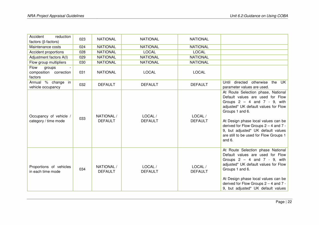
5.27. In Table 6.2.6, the approach that should be taken for each parameter is summarised
for the different stages of the life of a scheme. Parameters are either based on the
national default values or locally derived data. In a few instances, the existing UK
default values have been retained since there are insufficient data at present to
determine Irish parameters. Where it is indicated that the national default values are
to be adopted, the user must not change the values already contained within the
COBA program.
5.28. For each parameter, the COBA KEY number is provided: this corresponds directly
with the record on the COBA input deck.

NRA Project Appraisal Guidelines Unit 6.2:Guidance on Using COBA
Page | 21
Table 6.2.7: Summary Approach to Parameter Coding
PARAMETER COBA
KEY
PHASE 2 -
ROUTE
SELECTION
PHASE 3 DESIGN
/PHASE 5 ADVANCE
WORKS &
CONSTRUCTION
DOCUMENTS
PHASE 7
HANDOVER,
REVIEW &
CLOSEOUT
COMMENTS
Present value year /
appraisal period 003 NATIONAL NATIONAL NATIONAL
Traffic proportions 006 NATIONAL LOCAL LOCAL
Vehicle mix groups 007 NATIONAL LOCAL LOCAL
Seasonality index 008 NATIONAL LOCAL LOCAL
E-factor 008 NATIONAL LOCAL LOCAL
M-factor 008 NATIONAL LOCAL LOCAL
Growth of traffic 009 NATIONAL NATIONAL NATIONAL
Tax Rates 013 NATIONAL NATIONAL NATIONAL
Tax rate changes 014 NATIONAL NATIONAL NATIONAL .
Discount rate 015 NATIONAL NATIONAL NATIONAL
Vehicle operating cost 016 NATIONAL NATIONAL NATIONAL
Accident costs 017 NATIONAL NATIONAL NATIONAL
Annual compound
growth rates 019 NATIONAL NATIONAL NATIONAL
Annual compound
growth for fuel and non-
fuel
020 NATIONAL NATIONAL NATIONAL
Values of time per
person 021 NATIONAL NATIONAL NATIONAL
Accident rates, severity
splits for link / junction
combined
023 NATIONAL LOCAL LOCAL
NRA Project Appraisal Guidelines Unit 6.2:Guidance on Using COBA
Page | 22
Accident reduction
factors (β-factors) 023 NATIONAL NATIONAL NATIONAL
Maintenance costs 024 NATIONAL NATIONAL NATIONAL
Accident proportions 028 NATIONAL LOCAL LOCAL
Adjustment factors A(I) 029 NATIONAL NATIONAL NATIONAL
Flow group multipliers 030 NATIONAL NATIONAL NATIONAL
Flow groups -
composition correction
factors
031 NATIONAL LOCAL LOCAL
Annual % change in
vehicle occupancy 032 DEFAULT DEFAULT DEFAULT
Until directed otherwise the UK
parameter values are used.
Occupancy of vehicle /
category / time mode 033
NATIONAL /
DEFAULT
LOCAL /
DEFAULT
LOCAL /
DEFAULT
At Route Selection phase, National
Default values are used for Flow
Groups 2 – 4 and 7 - 9, with
adjusted* UK default values for Flow
Groups 1 and 6.
At Design phase local values can be
derived for Flow Groups 2 – 4 and 7 -
9, but adjusted* UK default values
are still to be used for Flow Groups 1
and 6.
Proportions of vehicles
in each time mode 034
NATIONAL /
DEFAULT
LOCAL /
DEFAULT
LOCAL /
DEFAULT
At Route Selection phase National
Default values are used for Flow
Groups 2 – 4 and 7 - 9, with
adjusted* UK default values for Flow
Groups 1 and 6.
At Design phase local values can be
derived for Flow Groups 2 – 4 and 7 -
9, but adjusted* UK default values

NRA Project Appraisal Guidelines Unit 6.2:Guidance on Using COBA
Page | 23
are still to be used for Flow Groups 1
and 6. Note when inputting
proportions for vehicle category 1
(normally cars), the flow group to
which the proportions relate must be
specified. Data for all the flow
groups used must be input.
Annual changes to
proportions in each time
mode for a particular
vehicle category
037 DEFAULT DEFAULT DEFAULT Until directed otherwise, the UK
parameter values are to be used.
Scheme costs 055 LOCAL LOCAL LOCAL
At Route Selection, Option
Comparison Estimate to be used.
At Design, the cost estimate should
be the weighted average of the
Target Cost 1 and Total Scheme
Budget.
If the Target Cost 2 estimate
produced at main contract award
phase exceeds the Target Cost 1
estimate, the CBA must be updated
accordingly.
The final outturn cost is to be used
for the purpose of Handover, Review
& Closeout CBA
* For details of adjustments refer to PAG Unit 6.3: TRL COBA Report

NRA Project Appraisal Guidelines Unit 6.2:Guidance on Using COBA
Page | 24
6 The COBA Input File
Format of Data Entry
Characters
6.1. Data are entered in the COBA input deck using individual ‘KEY’ records. Data items
may be divided into three groups:
• Alphanumeric (A): Contains any alphabetic, numeric or other character valid
to the computer.
• Real (R): Contains a number with a decimal point. If a decimal point is
omitted, COBA will assume its position is either on the right hand edge of the
box for numbers intrinsically greater than unity (for example flows), or at the
left hand edge for numbers intrinsically less than unity. This is indicated on
the coding sheets by the presence of a dot on one edge of the box. Blanks
(spaces) are treated as zeroes.
• Integer (I): Contains a number without a decimal point. Again, all blanks in
the box are interpreted as zeroes.
6.2. It should be noted that if a data field, which should contain a number, contains any
non-numeric character, (except a decimal point or minus sign where appropriate),
COBA will halt immediately with a computer system error. This is outside the control
of the COBA program.
Limits on Data
6.3. Most numeric data are required to be within certain limits. These limits are
principally to guard against mistyping of data in the wrong columns. If the data item
is discovered to be outside the limits shown in the description of that data item an
error message is printed; for example:
“This data item MUST NOT LIE OUTSIDE THE RANGE x TO y”.
6.4. Errors result in the Project being truncated to a data check only.
6.5. Some data items have two sets of limits, in which case the error limits are shown
with the warning limits in brackets. If the item is inside the error limits but outside the
warning limits, a warning message is printed; for example:
“WARNING - data item is LARGER THAN x”.
6.6. The warning limits are chiefly determined by the range of values of observations
made during the research on which COBA is based. The program will continue to run
to completion despite these warnings. Nevertheless, the user should review all such
warnings for each output provided, as they may point to coding errors.

NRA Project Appraisal Guidelines Unit 6.2:Guidance on Using COBA
Page | 25
Reclassification Repeat Inhibitor, RRI
6.7. In COBA there is a distinction between those improvements which would be made
whether or not the Do-Something were to be implemented (defined as the Do-
Minimum), and those which are alternatives to implementing the Do-Something.
6.8. Normally all reclassifications that occur in the Do-Minimum are repeated in each Do-
Something in the year in which they take effect in the Do-Minimum.
6.9. For each particular Do-Minimum mid-scheme data change, (that is, flow changes,
link or junction classification changes, or accident rate changes), it is possible to
prevent the repeat in each Do-Something by entering an ‘X’ in column 5. This ‘X’ is
referred to as the Reclassification Repeat Inhibitor, RRI. Obviously, the RRI is
meaningful only in a reclassification that occurs in the Do-Minimum. In all other
circumstances, it is ignored.
Link and Node Names
6.10. To a certain extent, link and node names are a matter of common sense. The values
permissible are numbers between 1 and 9999. Further limitations are imposed in
particular sections, for example:
• For a link or node to be classified or de-classified, or for its flow or accident
data to be specified, it must obviously be ‘in the network’;
• For a link or node to be declassified, it must first be classified;
• Connectivity between links and nodes must be preserved. In flow data if the
‘towards node’ is specified for a one-way link, it is obviously nonsensical if link
and node are not connected in the network. Similarly, during junction data,
the link on a subsequent record must refer to a link actually attached to the
node being classified;
• The list of the arms of a classified junction must correspond exactly to the
network description of that node; and
• The number of nodes that may be classified will generally be smaller than the
number of network nodes because of storage space limitations.
• To facilitate easy navigation through the link-node diagram, the link naming
convention should relate insofar as is practical to the adjacent node number.
For example, node 5 will have links 51, 52 and 53 connected to it. Node 38
will have links 381, 382 and 383 connected to it. The link connecting node 46
and 52 may be called either node 461 or 521. See Section 3.3 of PAG Unit
6.12: CBA Report for further elaboration.
Key Records
6.11. The COBA deck, defining a particular ‘Project’ is made up of a series of KEY
‘records’, which can be grouped together into the following headings:
• Control records;
• Basic data;
• Network data;

NRA Project Appraisal Guidelines Unit 6.2:Guidance on Using COBA
Page | 26
• Scheme data: declassification;
• Scheme data: costs;
• Scheme data: link flows;
• Scheme data: link classifications;
• Scheme data: node classifications;
• Scheme data: accidents; and
• Final control records.
6.12. Classification is the term used when a link or node is described by geometric
parameters in order that the costs of negotiating the link or node can be calculated.
Declassification is the process whereby the link or node can be retained in the
network but the user costs will no longer be calculated.
6.13. Following an overview of the format of the data entered into the COBA deck, this
section provides a summary of the contents of each of the above KEY categories.
However, a detailed description of how to code individual KEY ‘records’ in COBA is
found in DMRB Volume 13, Section 1, Part 7.
Control Records
6.14. Control records are used to highlight the data sections from each other, e.g. from the
basic records to the network data.
Basic Data
6.15. Basic Data are those data records that apply to the whole of the project; for example,
the years for which the Project is to be evaluated.
6.16. The order in which Basic Data records are entered is important since some items
interact with others. In general, entering records in the order of their free-format keys
will be successful, although the following guidelines should be noted:
• Mandatory records: KEYs 001, 003, 004 and 005 are mandatory records and
should be input in that order. If any of these records are omitted, then the
program run will be reduced to a Data Check Only. If the Print Phases
required are to be specified, then KEY 002 should be input in numerical order
within the mandatory records.
• Scheme years: COBA allows users to redefine the present value year on the
same record as the first and last scheme years (KEY 003 - mandatory). The
program will therefore not accept a Basic Data record of any type that
specifies a year unless the scheme years record has already been accepted.
Thus, since the KEY 003 record is mandatory (and is almost the first record of
a file), the program will only fail in this way if the record itself is unrecognised.
• Vehicle categories: Most COBA runs will be performed using the default set
of vehicle categories. If any item of Basic Data is entered which specifies a
vehicle category by number, COBA will assume this number refers to the
sequence of the default set. Thereafter the vehicle categories cannot be
redefined. The following Basic Data types relate to vehicle categories:
- Traffic proportions;

NRA Project Appraisal Guidelines Unit 6.2:Guidance on Using COBA
Page | 27
- Local growth factors;
- Adjustment factors;
- Occupancy and change in occupancy of category;
- Proportion of category in time mode; and
- Increment to vehicle mode split.
6.17. The essential point is that if vehicle categories are to be redefined, this must be done
before the traffic proportions for the project are specified.
Network Data
6.18. Network data are those records that define the structure of the Do-Minimum network
and how it changes with each scheme, or at reclassification years.
Scheme Data: Declassification
6.19. Declassification is the process whereby the link or node can be retained in the
network but the user costs will no longer be calculated.
Scheme Data: Costs
6.20. By convention, COBA costs are input for the whole Scheme at the very beginning of
the Scheme Data. Because of this, Scheme Costs will not be accepted in the
reclassification section. Values for scheme capital costs, traffic related maintenance
capital costs and delays during construction and maintenance works may be input in
present value year terms in the correct year on KEY 055.
6.21. It is an NRA requirement that KEY055 is used to enter costs. Detailed guidance on
how to derive the profile of scheme costs for input into COBA KEY055 can be found
in PAG Unit 6.7: Preparation of Scheme Costs.
Scheme Data: Link Flows
6.22. A single record is used to input link traffic flows, either as total vehicles or by vehicle
mix group. It is on this record that one-way links and their direction of flow are
defined.
Scheme Data: Link Classifications
6.23. These records are used to define the characteristics of all the links in the network for
which user cost calculations are required. Each link is defined by a separate record,
which allows the user to define the speed-flow relationship applicable to the link,
geometrical quantities such as lane widths, accident type and speed limits.
Scheme Data: Node Classifications
6.24. Those junctions that are classified are defined. Junction type, geometric parameters,
operational parameters (e.g. signal stages), delays and turning flows are entered.
Scheme Data: Accidents

NRA Project Appraisal Guidelines Unit 6.2:Guidance on Using COBA
Page | 28
6.25. Accident data must be the last data type entered into any Scheme Data section.
These data records are used to define observed accident rates or numbers, to
overwrite the default values held within the program. Links may have accident rates
only if they are classified.
Final Control Records
6.26. Control records define the end of scheme data, the end of the project data (when
more than one scheme) and the end of the program run.
Data Preparation and Editing
6.27. There are several methods a user can adopt to prepare the COBA input data file:
• An experienced user may prefer to edit an existing COBA input file;
• Entering data in the strict format defined in the COBA input coding sheets.
These require the user to enter each character of the input data into specific,
right-justified columns; or
• Using the program CSCREEN to edit an existing COBA input file or create a
new file in the COBA data format on screen. Some data checking is
undertaken as the file is created.
6.28. Edits to the data file can be done through a simple text editor. The file should be in
plain ASCII format (i.e. containing no special characters and each line terminating
with a carriage return). Suitable text editors include the NotePad or WordPad
program included with Windows software.
6.29. More sophisticated word processors may be used but the user must ensure that files
are saved as a plain text/text only file.
6.30. A default COBA input file is provided in PAG Unit 6.4: Default COBA Input File. This
file should be used as the starting point for coding. It contains all the default
parameter values discussed in previous Sections.
7 COBA Model Validation
Journey Time Validation Techniques
7.1. Often local journey time measurements over the road network will have been made
for the traffic modelling stage of scheme assessment. It is necessary to check
observed journey times with those on the assignment networks and those computed
by COBA. This comparison may bring to light specific instances where the COBA
Do-Minimum journey times no not adequately reflect observed values, or those
reported from the traffic models. (Note: COBA journey times for each flow group are
printed out for a specified year in Phase 8 of the COBA output).
7.2. Generally, journey times are only required on roads where there is likely to be
competition as a result of a network intervention. Given that the scheme benefits are

NRA Project Appraisal Guidelines Unit 6.2:Guidance on Using COBA
Page | 29
based largely on network journey time changes, it is necessary that the journey times
in COBA are accurately reflected on links where changes in traffic flow are expected.
7.3. Journey time measurements carried out for COBA should be used to estimate
average speeds only; it is not possible to determine the speed/flow slope to any
reasonable degree of confidence from a small-scale survey. The journey time
survey should be geared towards estimating observed journey time on the whole of
the bypassed section of route; individual estimates of speed on each link are not
required. In general, the longer the section of route that is being bypassed, the lower
should be the variability of observed journey times. Fewer observations should be
needed to estimate the journey time over a longer section of route to a given level of
accuracy.
7.4. The most important consideration for local journey time surveys is that the journey
times should be representative of conditions throughout the year. A large number of
runs carried out on one day will usually be worth less than fewer runs spread over
several days. Generally, measurements should be taken to cover both the peak and
off-peak hours of the day.
7.5. The moving observer method is the most widely used method of carrying out journey
time measurements. Alternatively, registration number surveys should be
considered as an alternative to the moving observer method – these have the
advantage of providing high sample rates. The NRA is open to alternative means of
collecting journey time information, once it can be demonstrated that the proposed
approach is representative.
7.6. The results of the journey time survey should be sent with the COBA Appraisal
Report and should include information on the number of runs carried out in each time
period with an estimate of their accuracy and details of the level of traffic flow at the
time. The survey results should be compared with the COBA modelled times and
flows in each flow group. If observed and modelled journey times are not in
reasonable agreement, then the speed/flow relationship that has been used for a
particular link should be reconsidered, and possibly a local relationship defined.
7.7. For full guidance on undertaking journey time surveys, and comparing with the model
output, reference should be made to DMRB Volume 13, Section 1, Part 5, Chapter
10 (Local Journey Time Measurements). PAG Unit 5.2: Construction of Transport
Models should be referred to for guidance on appropriate validation criteria for
journey times.
Junction Validation

NRA Project Appraisal Guidelines Unit 6.2:Guidance on Using COBA
Page | 30
7.8. Where junctions are explicitly modelled and COBA junction delay benefits are a
significant element of scheme benefits, the magnitude of the junction delay benefits
should be verified by considering the following:
• Do-Minimum improvements or, where Do-Something delays are large, Do-
Something junction optimisation. Small changes in the coding of junction
layouts can sometimes yield significant changes in junction delay costs;
• Comparison of COBA and measured journey times, for example, where
junctions interact. In practice, it is more common for local maximum average
delays to be less than 300 seconds rather than more; and
• Explicit modelling of critical junctions outside COBA. In exceptional cases,
the COBA user may wish to consider whether in-depth analysis of a critical
junction is necessary.
7.9. A particular problem with calibrating maximum delays using timed runs is that it is
impossible to calibrate future scenarios. For example, a junction may be coded at
300 seconds maximum delay on the basis of present journey time evidence, but may
give rise to longer delays in the future due to traffic growth. This may be tested using
more sophisticated junction modelling techniques as found in congested assignment
packages that explicitly model local diversionary reassignment. Advice from the
Strategic Planning Unit should be sought in such circumstances.
8 COBA Output and Interpretation
General
8.1. Historically, the COBA program has accepted input and worked in resource costs;
this is still the case with the Irish version of the software. However, the calculus
currently being used is the Willingness To Pay (WTP) methodology with the program
converting costs and benefits to market prices using appropriate tax correction
factors.
8.2. Following the COBA run, appraisal results are summarised at the end of the COBA
output file. The information describes the Economic Efficiency of the Transport
System and is expressed in Market Prices. This output is provided in the form of a
number of tables, each providing separate measures of output. The interpretation of
such output, and the processes behind the calculation of the performance indices is
described in this Section.
8.3. It is important to note that COBA is only able to allocate the elements of the appraisal
that the program calculates. There may be other significant costs and benefits that
should be included in the decision making process.
Sensitivity Testing
8.4. No COBA result is exact: a risk exists that project costs and benefits might deviate
from their expected values. Any investment decision, whether public or private
sector, is bound to be subject to uncertainty. Decisions regarding long-lived
investments with distant forecast horizons, such as national road proposals, are
subject to a high degree of uncertainty. However, it is important for decision makers

NRA Project Appraisal Guidelines Unit 6.2:Guidance on Using COBA
Page | 31
to have some idea about how robust the results may be in order to know what weight
to attach to them. It is, therefore, necessary to consider a range of possible
outcomes.
8.5. One approach is to set bounds on the uncertainty by carrying out tests on key
variables to identify those variables to which the results are particularly sensitive.
These are the variables on which the decision makers' judgment should focus.
Local Variables
8.6. At design, locally derived parameter values should be used where local data is both
reliable and significantly different from national values. However, it can be useful for
the user to carry out sensitivity tests on these variables, especially where they are
both uncertain in the local context and likely to affect the COBA result significantly.
8.7. It is recommended that any sensitivity test using local values should use the national
values as a benchmark. This is to ascertain the importance of local variations and to
allow comparison of schemes on a similar basis.

NRA Project Appraisal Guidelines Unit 6.2:Guidance on Using COBA
Page | 32
Forecasting Inputs
8.8. Errors introduced by economic forecasting inputs are known to have a significant
impact on NPV results, in particular the impact of Gross Domestic Product and
possibly fuel price assumptions on traffic forecasts and the associated values of
time, accidents and vehicle operating costs used in COBA. It is therefore necessary
to present COBA results based on high, medium and low traffic growth scenarios.
This should be done for all CBAs.
Scheme Costs
8.9. There is a great deal of uncertainty concerning the final capital costs of road
schemes. This degree of uncertainty tends to reduce at later stages of the project’s
development, when outturn costs can be estimated with more confidence. Sensitivity
tests should, therefore, be undertaken to assess the impact of changes in
construction costs and land and property costs on the overall NPV of a scheme (see
PAG Unit 6.1: Guidance on Conducting COBA for more detail). In particular the
testing should look at the impact of changing construction costs and the level of
change required to alter the viability of a scheme.
Other Considerations
8.10. It may well be the case that a sensitivity test highlights variation in the NPV, but that
the sign of the NPV and ranking of options remains unchanged. This would clearly
increase the weight that can be put on the economic results.
Interpretation of COBA Output
8.11. The most significant tables of the COBA output occur in Phase 16. These are:
Table 14, Phase 16 – ‘Conversion of Travel Costs to Market Prices by Vehicle
Category’
8.12. This table (see Table 6.2.7) shows the calculations necessary to convert the time
and vehicle operating cost changes calculated in resource costs to market prices.
The individual components given in Tables 9A to 9F of the COBA output file are
presented under the Transport Economic Efficiency (TEE) categories and converted
to market prices by the appropriate tax correction factors.
Table 15A, Phase 16 – ‘Economic Efficiency of the Road System in Market Prices
(TEE Table)’
8.13. Table 15A in the COBA output is an adaptation of the TEE Table. COBA takes the
input values for the construction delays and maintenance delay savings (expressed
as resource costs), converts to market prices and allocates between ‘consumers’
and ‘business’ in proportion to the consumer and business user (Time and VOC)
benefits of the scheme under normal operating conditions.
8.14. Table 6.2.8 shows how the elements of the TEE Table calculated by COBA are
referenced from Table 14 and combined with the delays during construction and

NRA Project Appraisal Guidelines Unit 6.2:Guidance on Using COBA
Page | 33
maintenance delay savings to produce the ‘Net Consumer User Benefit’ and ‘Net
Business Impact’.
Table 15B, Phase 16 – ‘Public Accounts’
8.15. This Table (see Table 6.2.9) shows the summary of Public Accounts and
summarises the funding of the project. This table fulfils the requirement for an
“exchequer cash flow analysis”.
Table 15C, Phase 16 – ‘Analysis of Monetised Costs and Benefits’
8.16. Table15C (shown in Table 6.2.10) of the COBA output summarises the monetised
costs and benefits as calculated by COBA. This effectively represents the scheme
summary, and is the key output from the CBA assessment.

NRA Project Appraisal Guidelines Unit 6.2:Guidance on Using COBA
Page | 34
Table 6.2.7: Conversion of travel costs to market prices by vehicle category (Table
14, Phase 16 of the COBA Output)
From
Table
VEHICLE
CATEGORY
TIME TOTAL
TIME
OPERATING
FUEL
OPERATING
OTHER
TOTAL
OPER.
COSTS WORK COMM/OTHER WORK COMM/
OTHER
WORK COMM/
OTHER
9A
9B
9E
Personal
Travel
Car
Private LGV
TOTAL
Adjustment
MARKET
PRICE
PSV
Adjustment
MARKET
PRICE
-
Σ
Σ × t
Σ= AA
Σ × t
Σ= GG
Σ
Σ × t
Σ= BB
Σ × t
Σ= HH
Σ
Σ(row)
Σ
Σ(row)
Σ=
Σ see note
vi
Σ= CC
-
Σ
Σ × tF
Σ= DD
-
Σ
Σ × t
Σ= EE
-
Σ
Σ × tN
Σ= FF
-
Σ
Σ(row)
Σ
-
9B
9C
9D
Freight
Freight LGV
OGV1
OGV2
TOTAL
Adjustment
MARKET
PRICE
Σ
Σ × t
Σ= II
-
Σ
Σ(row)
Σ
Σ see note
vi
Σ= JJ
-
Σ
Σ × t
Σ= KK
-
Σ
Σ(row)
Σ
9E
Private
Sector
PSV
Adjustment
MARKET
PRICE
Σ × t
Σ=LL
-
Σ(row)
Σ
see note
vi
Σ= MM
-
Σ × t
Σ= NN
-
Σ(row)
Σ
Totals Σ Σ Σ Σ Σ Σ Σ Σ
THIS ANALYSIS IS BASED ON ………………… TRAFFIC GROWTH
AND ………………… ECONOMIC GROWTH
COSTS ARE IN ( PV Year ) PRICES IN MULTIPLES OF A THOUSAND EURO AND ARE DISCOUNTED TO (PV
Year)
EVALUATION PERIOD (evaluation period ) YEARS FIRST SCHEME YEAR …… CURRENT YEAR ……
DISCOUNT RATE (discount rate) PERCENT FOR (years) YEARS THEREAFTER (discount rate) for
(years)
THEREAFTER (discount rate) PERCENT
Notes:
(i) ‘t’ is the average rate of indirect tax on final consumption in the economy; (ii) ‘tF’ is the rate of indirect tax on fuel as a final consumption good;
(iii) ‘tF∋’ is the rate of indirect tax on fuel as an intermediate consumption good;
(iv) ‘tN’ is the rate of indirect tax on non-fuel vehicle operating costs as a final consumption good; (v) ‘tN∋’ is the rate of indirect tax on non-fuel vehicle operating costs as an intermediate
consumption good; (vi) The adjustment for Working Operating Fuel is Σ Total x ( 1 + t N∋ ) × ( 1 + t ) - Σ Total

NRA Project Appraisal Guidelines Unit 6.2:Guidance on Using COBA
Page | 35
Table 6.2.8: Economic efficiency of the road system in market prices (Table 15A,
Phase 16 of the COBA Output)
IMPACT TABLE REF TOTAL CARS &
PRIVATE
LGVs
GOODS
VEHS &
BUS.
LGVs
BUS AND
COACH
CONSUMER USER BENEFITS
User Benefits
Travel Time
Vehicle operating costs
Travel time and vehicle operating costs
During construction
During maintenance
=Σ (row)
=Σ (row)
See note
(i)
See note
(i)
BB
DD + FF
-
-
-
-
HH
-
NET CONSUMER USER BENEFITS (1) =Σ
(column) Σ - Σ
BUSINESS USERS
User Benefits
Travel Time
Vehicle operating costs
Travel time and vehicle operating costs
During construction
During maintenance
Subtotal
Private Sector Provider Impacts
Operating Costs
Other Business Impacts
Developer and Other
Contributions
(2)
(3)
(4)
=Σ (row)
=Σ (row)
See note
(i)
See note
(i)
=Σ (row)
AA
CC + EE
II
JJ + KK
GG + LL
-
MM + NN
NET BUSINESS IMPACT (5) = (2)+
(3)+ (4) Σ Σ Σ Σ
TOTAL Present Value of Transport
Economic Efficiency Benefits
(6) = (1) + (5) Σ
THIS ANALYSIS IS BASED ON ………………… TRAFFIC GROWTH
AND ………………… ECONOMIC GROWTH
COSTS ARE IN ( PV Year ) PRICES IN MULTIPLES OF A THOUSAND EURO AND ARE DISCOUNTED TO (PV
Year)
EVALUATION PERIOD (evaluation period ) YEARS FIRST SCHEME YEAR …… CURRENT YEAR ……
DISCOUNT RATE (discount rate) PERCENT FOR (years) YEARS THEREAFTER (discount rate) for
(years)
THEREAFTER (discount rate) PERCENT
Notes:
(i) COBA takes the input values for the Construction Delays and Maintenance delay Savings, converts to market prices (multiplies by 1 + t ) and allocates between ‘Consumers’ and ‘Business’ in proportion to the Consumer and business User (Time and VOC) benefits of the scheme under normal operating conditions.
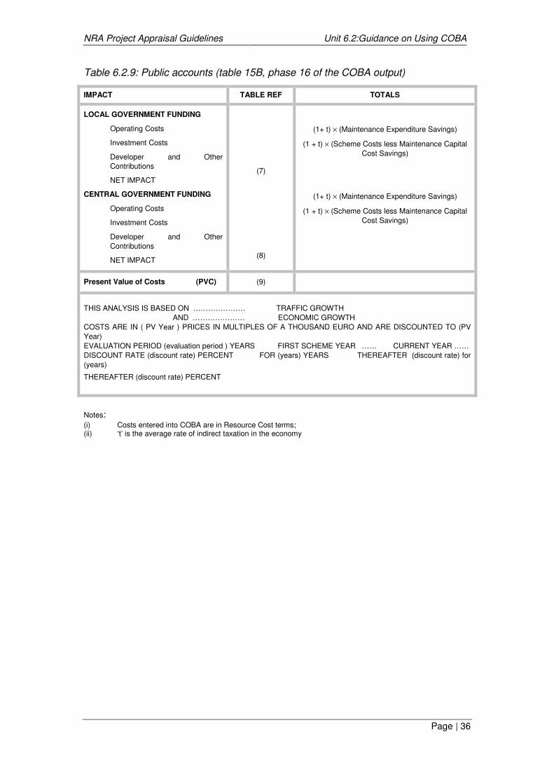
NRA Project Appraisal Guidelines Unit 6.2:Guidance on Using COBA
Page | 36
Table 6.2.9: Public accounts (table 15B, phase 16 of the COBA output)
IMPACT TABLE REF TOTALS
LOCAL GOVERNMENT FUNDING
Operating Costs
Investment Costs
Developer and Other
Contributions
NET IMPACT
CENTRAL GOVERNMENT FUNDING
Operating Costs
Investment Costs
Developer and Other
Contributions
NET IMPACT
(7)
(8)
(1+ t) × (Maintenance Expenditure Savings)
(1 + t) × (Scheme Costs less Maintenance Capital
Cost Savings)
(1+ t) × (Maintenance Expenditure Savings)
(1 + t) × (Scheme Costs less Maintenance Capital
Cost Savings)
Present Value of Costs (PVC) (9)
THIS ANALYSIS IS BASED ON ………………… TRAFFIC GROWTH
AND ………………… ECONOMIC GROWTH
COSTS ARE IN ( PV Year ) PRICES IN MULTIPLES OF A THOUSAND EURO AND ARE DISCOUNTED TO (PV
Year)
EVALUATION PERIOD (evaluation period ) YEARS FIRST SCHEME YEAR …… CURRENT YEAR ……
DISCOUNT RATE (discount rate) PERCENT FOR (years) YEARS THEREAFTER (discount rate) for
(years)
THEREAFTER (discount rate) PERCENT
Notes: (i) Costs entered into COBA are in Resource Cost terms; (ii) ‘t’ is the average rate of indirect taxation in the economy

NRA Project Appraisal Guidelines Unit 6.2:Guidance on Using COBA
Page | 37
Table 6.2.10: Analysis of monetised costs and benefits (table 15C, phase 16 of the
COBA output)
IMPACT TABLE REF TOTALS
TEE Benefits
Consumer User Benefits
Business Benefits
Private Sector Provider Impacts
Accident Benefits
Emission Benefits
Indirect Tax benefit
Residual Value
(1)
(2)
(3)
(10)
(11)
(12)
(13)
Present Value of Benefits (PVB) (14) Σ
Government Funding
Present value of Costs (PVC)
(9)
Overall Impact
Net Present Value (NPV)
Benefit to Cost Ratio (BCR)
(14) – (9)
(14) / (9)
THIS ANALYSIS IS BASED ON ………………… TRAFFIC GROWTH
AND ………………… ECONOMIC GROWTH
COSTS ARE IN ( PV Year ) PRICES IN MULTIPLES OF A THOUSAND EURO AND ARE DISCOUNTED TO (PV
Year)
EVALUATION PERIOD (evaluation period) YEARS FIRST SCHEME YEAR …… CURRENT YEAR ……
DISCOUNT RATE (discount rate) PERCENT FOR (years) YEARS THEREAFTER (discount rate) for
(years)
THEREAFTER (discount rate) PERCENT
Note: There may also be other significant costs and benefits, some of which cannot be presented in monetised form.
Where this is the case, the analysis presented above does NOT provide a complete measure of value for money
and should not be used as the sole basis for decisions