project 1 - carnegie mellon school of computer science15869-f10/lec/05/lec05.pdf · hair simulation...

Project 1

Bren Meeder Heegun Lee

• Has been posted!

• Previous year projects:

Sunday, October 3, 2010

Hair Simulation(and Rendering)

Adrien Treuille

Image from Final Fantasy (Kai’s hair)


Overview•More Constraints

•Hair• Real Hair

• Questions

• Hair Dynamics

• Hair Rendering


SG4

Example: Point-on-circle

Write down the constraint equation.

Take the derivatives.

Substitute into generic template, simplify.

C = x - r

N = !C

!x = x

x

N = !2C

!x!t = 1

x x -

x"xx"x

x

# = -mN"x

N"N -

N"f

N"N = m

( )x"x 2

x"x - m( )x"x - x"f 1

x

Drift and Feedback

• In principle, clamping at zero is enough

• Two problems:

– Constraints might not be met initially

– Numerical errors can accumulate

• A feedback term handles both problems:

C = - $C - %C, instead of

C = 0

C

$ and % are magic constants.

Tinkertoys

• Now we know how to simulate a bead on a wire.

• Next: a constrained particle system.

–E.g. constrain particle/particle distance to make rigid links.

• Same idea, but…

Constrained particle systems

• Particle system: a point in state space.

• Multiple constraints:

– each is a function Ci(x1,x2,…)

– Legal state: Ci= 0, & i.

– Simultaneous projection.

– Constraint force: linear combination of constraint gradients.

• Matrix equation.


SG5

Compact Particle System Notation

q: 3n-long state vector.

Q: 3n-long force vector.

M: 3n x 3n diagonal mass matrix.

W: M-inverse (element- wise reciprocal)

q = x1,x2, ,xn

Q = f1,f2, ,fn

M =

m1

m1

m1

mn

mn

mn

W = M-1

q = WQ

Particle System Constraint Equations

C = C1,C2, ,Cm

! = !1,!2, ,!m

J = "C

"q

J = "2C

"q"t

q = W Q + JT!

Matrix equation for !

Constrained Acceleration

More Notation

Derivation: just like bead-on-wire.

JWJT ! = -Jq - JW Q

How do you implement all this?

• We have a global matrix equation.

• We want to build models on the fly, just like masses and springs.

• Approach:

– Each constraint adds its own piece to the equation.

Matrix Block Structure

C

x i

x j

J

• Each constraint contributes one or more blocks to the matrix.

• Sparsity: many empty blocks.

• Modularity: let each constraint compute its own blocks.

• Constraint and particle indices determine block locations.

"C

"x i

"C

"x j

SG5






q = x1,x2, ,xn

Q = f1,f2, ,fn

M =

m1

m1

m1

mn

mn

mn

W = M-1

q = WQ


C = C1,C2, ,Cm

! = !1,!2, ,!m

J = "C

"q

J = "2C

"q"t

q = W Q + JT!



More Notation


JWJT ! = -Jq - JW Q




• Approach:



C

x i

x j

J





"C

"x i

"C

"x j


Constrained Dynamics:

stat

eco

nstr

aint

svi

rtua

l wor

kth

eref

ore

T |due to f = x · f = 0

d

dtx = x

T = x ·�f + f

�

C(x) = 0

d

dtx = x = M−1

�f + f

�= W

�f + f

�

C = J x + J x = 0

= J x + JW�f + f

�

C =dCdt

=∂C∂x

x = J x = 0

∴ JW f = −J x− JW f

∴ f = JT λ

JWJT λ = −J x− JW f

∴ λ =�JWJT

�−1�−J x− JW f

�

At any point the set of legal velocities are those which are perpendicular to the rows of J.

Conversely, the illegal velocities are spanned by JT i.e. {JT! | ! ! Rc}.

Since the constraint force is perpendicular to all legal velocities,

it must be in the span of JT.

General Case

T =12xT M x

T = xT M x


SG4

Example: Point-on-circle

Write down the constraint equation.

Take the derivatives.

Substitute into generic template, simplify.

C = x - r

N = !C

!x = x

x

N = !2C

!x!t = 1

x x -

x"xx"x

x

# = -mN"x

N"N -

N"f

N"N = m

( )x"x 2

x"x - m( )x"x - x"f 1

x

Drift and Feedback

• In principle, clamping at zero is enough

• Two problems:

– Constraints might not be met initially

– Numerical errors can accumulate

• A feedback term handles both problems:

C = - $C - %C, instead of

C = 0

C

$ and % are magic constants.

Tinkertoys

• Now we know how to simulate a bead on a wire.

• Next: a constrained particle system.

–E.g. constrain particle/particle distance to make rigid links.

• Same idea, but…

Constrained particle systems

• Particle system: a point in state space.

• Multiple constraints:

– each is a function Ci(x1,x2,…)

– Legal state: Ci= 0, & i.

– Simultaneous projection.

– Constraint force: linear combination of constraint gradients.

• Matrix equation.


SG5






q = x1,x2, ,xn

Q = f1,f2, ,fn

M =

m1

m1

m1

mn

mn

mn

W = M-1

q = WQ


C = C1,C2, ,Cm

! = !1,!2, ,!m

J = "C

"q

J = "2C

"q"t

q = W Q + JT!



More Notation


JWJT ! = -Jq - JW Q




• Approach:



C

x i

x j

J





"C

"x i

"C

"x j


SG6

Global and Local

C

! fc

x

v

fm

x

v

fm

Constraint

Global Stuff

J J&

C&

Constraint Structure

x

v

f

m

x

v

fm

p2

p1

C = x1 - x2 - r

"C

"x1

, "C

"x2

"2C

"x1"t, "2C

"x2"t

C C

Distance Constraint

Each constraintmust know howto compute these

Constrained Particle Systems

x

v

f

m

x

v

f

m

…

x

v

f

m

particles n time forces nforces

… FFF F F

consts nconsts

CCCCC …

Added Stuff

Modified Deriv Eval Loop

… FFF F F

Clear ForceAccumulators

Apply forces

x

v

f

m

x

v

f

m

…

x

v

f

m

x

v

fm

x

v

fm

…

x

v

fm

Return to solver

1

2

4CCCCC …

Compute and applyConstraint Forces

3

Added Step


SG7

Constraint Force Eval

• After computing ordinary forces:

– Loop over constraints, assemble

global matrices and vectors.

– Call matrix solver to get !, multiply

by to get constraint force.

– Add constraint force to particle

force accumulators.

JT

Impress your Friends

• The requirement that constraints not add or

remove energy is called the Principle of

Virtual Work.

• The !’s are called Lagrange Multipliers.

• The derivative matrix, J, is called the

Jacobian Matrix.

A whole other way to do it.

x = r cos ",sin "

I. Implicit:

II. Parametric:

C(x) = x - r = 0

Point-on-circle

"

x

Parametric Constraints

x = r cos ",sin "

Point-on-circle

"

x

• Constraint is always met exactly.

• One DOF: ".

• Solve for ."

Parametric:




• Questions

• Hair Dynamics

• Hair Rendering


Real Hair


Real Hair

• Typical human head has 150k-200k individual strands.

• Dynamics not well understood.

• Subject still open to debate.

Figure 1.1: Left, close view of a hair fiber (root upwards) showing the cuticlecovered by overlapping scales. Right, bending and twisting instabilities observedwhen compressing a small wisp.

Deformations of a hair strand involve rotations that are not infinitely small andso can only be described by nonlinear equations [AP07]. Physical effects arisingfrom these nonlinearities include instabilities called buckling. For example, whena thin hair wisp is held between two hands that are brought closer to each other(see Figure 1.1, right), it reacts by bending in a direction perpendicular to theapplied compression. If the hands are brought even closer, a second instabilityoccurs and the wisp suddenly starts to coil (the bending deformation is convertedinto twist).

1.3 Oriented Strands: a versatile dynamic primitive

The simulation of strand like primitives modeled as dynamics of serial branchedmulti-body chain, albeit a potential reduced coordinate formulation, gives rise tostiff and highly non-linear differential equations. We introduce a recursive, lineartime and fully implicit method to solve the stiff dynamical problem arising fromsuch a multi-body system. We augment the merits of the proposed scheme bymeans of analytical constraints and an elaborate collision response model. Wefinally discuss a versatile simulation system based on the strand primitive forcharacter dynamics and visual effects. We demonstrate dynamics of ears, braid,long/curly hair and foliage.

15




• Questions

• Hair Dynamics

• Hair Rendering


Questions• How could we simulate hair?

• What about...

• ...preventing bending?

• ...different kinds of hair?

• ...collisions?

• ...200k hairs?


Student Answers- hair models - mass-spring model: string of particles (one attached to scalp) - but we need a length constraint! - prevent bending: attach every two particles - use constraints to prevent over stretching - how about more than one strand per hair - simulate torsion - rather than using just straight lines, could we use bezier curves as basic elements - rather than using individual strands, interpolate a general mesh- how to implement curly hair: - put the particles in a helix and try to revert to that position - attach every nth particle - force a "curl" - equally favors clockwise and counterclockwise curls - use "big particles" that won't collide at a distance- adjusting the number of particles may affect the hair dynamics (beyond just increasing resolution)- for collisions - implement a spatial data structure to save computation - repelling forces, but could be an issue for many particles - have soft spring forces when "cylinders" intersect- to achieve 100k strands - interpolate between hairs - extrapolate from one hair to many




• Questions

• Hair Dynamics

• Hair Rendering


Hair Dynamics

•Control Mesh

•Mass-Spring Systems

•Rigid Links

•Super Helices


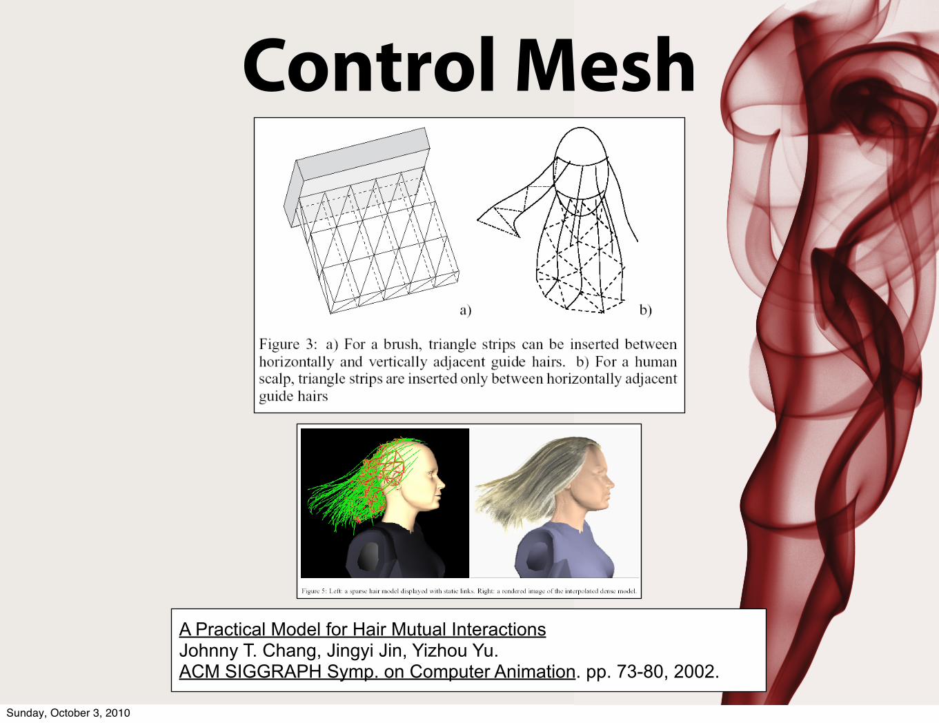
Control Mesh

A Practical Model for Hair Mutual InteractionsJohnny T. Chang, Jingyi Jin, Yizhou Yu.ACM SIGGRAPH Symp. on Computer Animation. pp. 73-80, 2002.


Control Mesh


Hair Dynamics

•Control Mesh


•Rigid Links

•Super Helices


Recall...


Disadvantages

• Torsional Rigidity

• Non-stretching of the strands


We decided to start with the mass-spring system since we had a working code fromthe in-house cloth simulator. There we started by adapting the existing particle-based simulator to hair.

mass-spring structure for hair

Figure 5.18: Mass spring structure for hair simulation

In our simulator, each hair would be represented by a number of nodes, each noderepresenting the (lumped) mass of certain portion of hair. In practice, each CVof guide hairs (created at the grooming stage) was used as the mass node. Suchnodes are connected by two types of springs - linear and angular springs. Linear

132


Implicit integrator adds stabilityLoss of angular momentum ‘Good’ Jacobian (filter) very important

k = ∞

n+1

implicit integration?


Well, how do we preserve length then?

use non-linear correction

k Is infinity!


non-linear post correction



Post solve correction Successive relaxation until

convergence Guaranteed length preservation

Cheap simulation of kinfinity



How to implement? Cloth simulation literatures

Provot 1995 (position only) Bridson 2002 (impulse)

Hair-specific relaxation possible


Predictor-corrector scheme

Implicit Filter (Predictor)

Sharpener (Corrector)

Implicit Filter (Predictor)


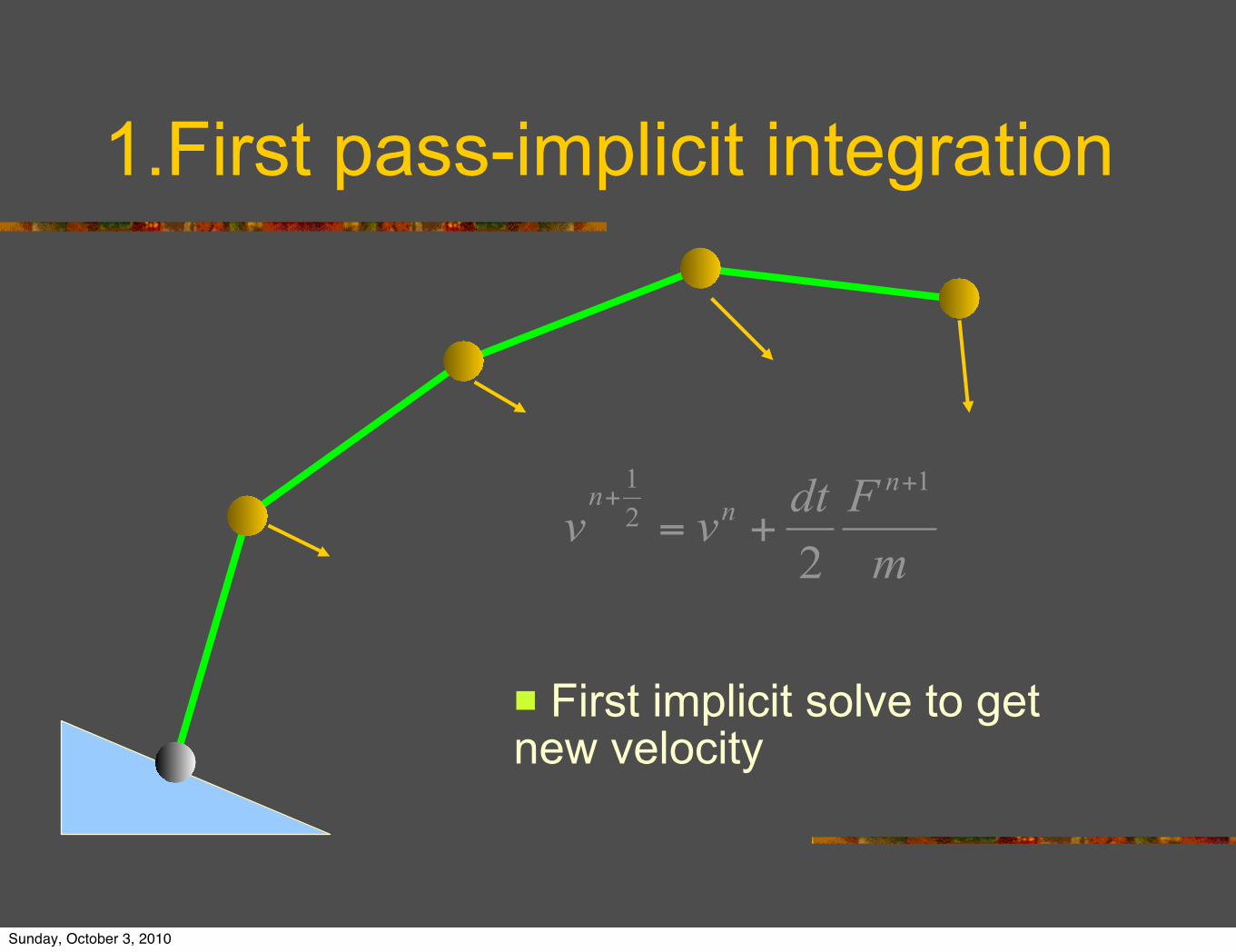
1.First pass-implicit integration

First implicit solve to get new velocity


2.First pass-implicit integration

Advance position with the predicted mid-step velocity


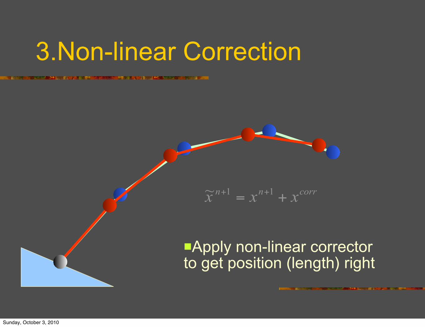
3.Non-linear Correction

Apply non-linear corrector to get position (length) right


4.Impulse

Change velocity due to length preservation

Velocity may be out of sync after impulse


5.Second implicit integration

Filters out velocity field

Velocity field in sync again


Hair Dynamics

•Control Mesh


•Rigid Links

•Super Helices


Featherstone Algorithm

inboardjoint

outboardjoint

O

link i!1

fI

i!1

fOi!1 !O

i!1

gmi!1

!Ii!1

link 0(base)

link 1

link i

link n

joint 1

joint ijoint i+1

joint n

outboardinboard


Rigid Links

• Fewer degrees of freedom.

• Torsional forces.

• Difficult Implementation.

• Constraints Difficult.


Hair Dynamics

•Control Mesh


•Rigid Links

•Super Helices


Super Helicesother interesting approaches to handle strand-strand interactions include wisp levelinteractions [PCP01b, BKCN03b], layers [LK01b] and strips [CJY02b].

We demonstrate the effectiveness of the proposed Oriented Strand methodology,through impressive results in production of Madagascar and Shrek The Third atPDI/DreamWorks, in Section 5.1.

1.4 Super-Helices: a compact model for thin geometry

Figure 1.5: Left, a Super-Helix. Middle and right, dynamic simulation of naturalhair of various types: wavy, curly, straight. These hairstyles were animated usingN = 5 helical elements per guide strand.

The Super-Helix model is a novel mechanical model for hair, dedicated to the ac-curate simulation of hair dynamics. In the spirit of work by Marschner et al. in thefield of hair rendering [MJC+03a], we rely on the structural and mechanical fea-tures of real hair to achieve realism. This leads us to use Kirchhoff equations fordynamic rods. These equations are integrated in time thanks to a new deformablemodel that we call Super-Helices: A hair strand is modeled as a C

1 continuous,piecewise helical1 rod, with an oval to circular cross section. We use the degreesof freedom of this inextensible rod model as generalized coordinates, and derivethe equations of motion by Lagrangian mechanics. As our validations show, theresulting model accurately captures the nonlinear behavior of hair in motion, whileensuring both efficiency and robustness of the simulation.

This work was published at SIGGRAPH in 2006 [BAC+06], and results from acollaboration with Basile Audoly, researcher in mechanics at Universite Pierre etMarie Curie, Paris 6, France.

1A helix is a curve with constant curvatures and twist. Note that this definition includes straightlines (zero curvatures and twist), so Super-Helices can be used for representing any kind of hair.

33

Why just use straight rods?


Super Helices

we found that slight variations of (κn

i (s))i with s allow for more realistic hair

styles. Finally, we choose for the dissipation energy D in equation (1.24d) a simple

heuristic model for capturing visco-elastic effects in hair strands, the coefficient γbeing the internal friction coefficient.

All the terms needed in equation (1.23) have been given in equations (1.24). By

plugging the latter into the former, one arrives at explicit equations of motion

for the generalized coordinate q(t). Although straightforward in principle, this

calculation is involved3. It can nevertheless be worked out easily using a symbolic

calculation language such as Mathematica [Wol99]: the first step is to implement

the reconstruction of Super-Helices as given in Appendix 1.4.3; the second step

is to work out the right-hand sides of equations (1.24), using symbolic integration

whenever necessary; the final step is to plug everything back into equation (1.23).

This leads to the equation of motion of a Super-Helix:

M[s,q] · q+K · (q−qn) = A[t,q, q]+� L

0

JiQ[s,q, t] · Fi(s, t)ds. (1.25)

In this equation, the bracket notation is used to emphasize that all functions aregiven by explicit formula in terms of their arguments.

In equation (1.25), the inertia matrix M is a dense square matrix of size 3N,

which depends nonlinearly on q. The stiffness matrix K has the same size, is

diagonal, and is filled with the bending and torsional stiffnesses of the rod. The

vector qndefines the rest position in generalized coordinates, and is filled with

the natural twist or curvature κn

i of the rod over element labelled Q. Finally,

the vector A collects all remaining terms, including air drag and visco-elastic

dissipation, which are independent of q and may depend nonlinearly on q and q.

Time discretization

The equation of motion (1.25) is discrete in space but continuous in time. For

its time integration, we used a classical Newton semi-implicit scheme with fixed

time step. Both the terms q and q in the left-hand side are implicited. Every

time step involves the solution of a linear system of size 3N. The matrix of this

linear system is square and dense, like M, and is different at every time step: a

3The elements of M, for instance, read MiQ,i�Q� = 1

2

��JiQ(s,q) ·Ji�Q�(s�,q)dsds� where J is the

gradient of rSH(s,q) with respect to q.

38

1.4.1 The Dynamics of Super-Helices

Figure 1.6: Left, geometry of Super-Helix. Right, animating Super-Helices with

different natural curvatures and twist: a) straight, b) wavy, c) curly, d) strongly

curly. In this example, each Super-Helix is composed of 10 helical elements.

We shall first present the model that we used to animate individual hair strands

(guide strands). This model has a tunable number of degrees of freedom. It is

built upon the Cosserat and Kirchhoff theories of rods. In mechanical engineering

literature, a rod is defined as an elastic material that is effectively one dimensional:

its length is much larger than the size of its cross section.

Kinematics

We consider an inextensible rod of length L. Let s ∈ [0,L] be the curvilinear

abscissa along the rod. The centerline, r(s, t), is the curve passing through the

center of mass of every cross section. This curve describes the shape of the rod at

a particular time t but it does not tell how much the rod twists around its centerline.

In order to keep track of twist, the Cosserat model introduces a material frame

ni(s, t) at every point of the centerline2. By material, we mean that the frame

‘flows’ along with the surrounding material upon deformation. By convention, n0

is the tangent to the centerline:

r�(s, t) = n0(s, t), (1.20a)

2By convention, lowercase Latin indices such as i are used for all spatial directions and run

over i = 0,1,2 while Greek indices such as α are for spatial directions restricted to the plane of

the cross section, α = 1,2.

34


Super Helices

Figure 1.8: Fitting γ for a vertical oscillatory motion of a disciplined, curly hair

clump. Left, comparison between the real (top) and virtual (bottom) experiments.

Right, the span �A of the hair clump for real data is compared to the simulations

for different values of γ . In this case, γ = 1.10−10

kg · m3 · s

−1gives qualitatively

similar results.

natural hair. We used the technique presented previously to fit the parameters of

the Super Helix from the real manipulated hair clump. As shown in Figure 1.9,

left, our Super-Helix model adequately captures the typical nonlinear behavior

of hair (buckling, bending-twisting instabilities), as well as the nervousness of

curly hair when submitted to high speed motion (see Figure 1.8, left). Figure 1.9,

right, shows the fast motion of a large hair, which is realistically simulated using

3 interacting Super-Helices. All these experiments also allowed us to check the

stability of the simulation, even for high speed motion.

Finally, Figure 1.10 demonstrates that our model convincingly captures the com-

plex effects occurring in a full head of hair submitted to a high speed shaking

motion.

43


Super Helices




• Questions

• Hair Dynamics

• Hair Rendering


We decided to start with the mass-spring system since we had a working code fromthe in-house cloth simulator. There we started by adapting the existing particle-based simulator to hair.

mass-spring structure for hair

Figure 5.18: Mass spring structure for hair simulation

In our simulator, each hair would be represented by a number of nodes, each noderepresenting the (lumped) mass of certain portion of hair. In practice, each CVof guide hairs (created at the grooming stage) was used as the mass node. Suchnodes are connected by two types of springs - linear and angular springs. Linear

132


Rendering

associated with the numerical integration of the Kirchhoff equa-tions, which are numerically very stiff. They propose an attemptfor removing this stiffness. It brings a very significant improvementover previous methods but we found that it was still insufficientfor hair animation purposes: there remain quite strong constraintson the time steps compatible with numerical stability of the algo-rithm. For instance, simulation of a 10 cm long naturally straighthair strand using the algorithm given in [Hou et al. 1998] remainedunstable even with 200 nodes and a time step as low as 10!5 s. Thestiffness problems in nodal methods have been analyzed in depthby [Baraff and Witkin 1992] who promoted the use of Lagrangiandeformable models (sometimes called ‘global models’ as opposedto nodal ones). This is indeed the approach we used above to de-rive the Super-Helix model, in the same spirit as [Witkin and Welch1990; Baraff and Witkin 1992; Qin and Terzopoulos 1996].

We list a few key features of the Super-Helix model which con-tribute to realistic, stable and efficient hair simulations. All spaceintegrations in the equations of motion are performed symbolicallyoff-line, leading to a quick and accurate evaluation of the coeffi-cients in the equation of motion at every time step. The inextensibil-ity constraint, enforced by equations (1a–1b), is incorporated intothe reconstruction process. As a result, the generalized coordinatesare free of any constraint and the stiff constraint of inextensibilityhas been effectively removed from the equations. Moreover, themethod offers a well-controlled space discretization based on La-grangian mechanics, leading to stable simulations even for small N.For N " !, the Kirchhoff equations are recovered, making the sim-ulations very accurate. By tuning the parameter N, one can freelychoose the best compromise between accuracy and efficiency, de-pending on the complexity of hair motion and on the allowed com-putational time. We are aware of another Lagrangian model4 usedin computer graphics that provides an adjustable number of de-grees of freedom, namely the Dynamic NURBS model [Qin andTerzopoulos 1996], studied in the 1D case by [Nocent and Remion2001]. Finally, external forces can have an arbitrary spatial depen-dence and do not have to be applied at specific points such as nodes,thereby facilitating the combination with the interaction model.

4 Application and validation

In this section, our Super-Helix model is used to animatesparse guide strands that define global hair motion, in a simi-lar way to [Daldegan et al. 1993; Chang et al. 2002]. A newscheme is first proposed for convincingly modelling a hair as-sembly from this sparse set of guide strands. Then, we pro-vide a validation of our physical model against a series of ex-periments on real hair, and demonstrate that the Super-Helixmodel accurately simulates the motion of hair. Images andvideos showing our set of results are available at http://www-evasion.imag.fr/Publications/2006/BACQLL06/.

4.1 Modelling a hair assembly

Sparse set of guide hair strands: Realistically animating hairfrom only a few hundreds of simulated strands is made possible bythe local coherence of hair motion. As in previous approaches, thepresent model aims at mimicking the collective behavior of hair bysetting up adequate interaction forces between the simulated strands(Super-Helices) and by adding extra strands at the rendering stage.

4In this model, geometric parameters, defined by the NURBS controlpoints and the associated weights, are used as generalized coordinates inthe Lagrangian formalism. In contrast, we opt here for mechanically-basedgeneralized coordinates: they are the values of the material curvatures andtwist, which are the canonical unknowns of the Kirchhoff equations.

In the following, we briefly explain how hair interactions are han-dled, and propose a unified scheme for generating the hair geometryfrom the set of sparse guide strands.

Hair interactions: Simulating a full head of hair requires an ef-ficient and accurate scheme for handling hair-hair and hair-bodycollisions. Detection is efficiently processed by exploiting tempo-ral coherence, as in [Raghupathi et al. 2003]: we avoid the quadraticcost of computing proximity of guide strands by keeping track ofpairs of closest points over time. As in [Choe et al. 2005], contactsbetween hair volumes are handled by dissipative penalty forces.

Generating the rendered hair geometry: To be able to han-dle both smooth and clumpy hairstyles, we avoid choosing betweencontinuum and wisp-based representations for hair. Many realhairstyles display an intermediate behavior with hair strands beingmore evenly spaced near the scalp than near the tips. Our solutionis based on a semi-interpolating scheme to generate non-simulatedhair strands from the guide strands (see Figure 4, and the video):we range from full interpolation to generate the extra hair strandsnear the scalp to no interpolation within a hair wisp near the tips.The separation strongly depends on the level of curliness: straighthair requires more interpolation than curly and clumpy hair. Notethat for smooth, interpolated hair, we avoid interpolation betweentwo guide strands having close roots but distant tips by adding acriterion on the distance between tips, see Figure 4, (d).

Figure 4: Semi-interpolating scheme for generating the final hairgeometry: hair a) is smoothly interpolated, b) is interpolated nearthe roots but clumpy near the tips, c) forms disjoint locks (no inter-polation); d) interpolation across the right shoulder is prevented bythe criterion on the maximal distance between the tips.

In our animations, the final hair geometry was rendered using themodel of Marschner et al. [2003] for accurately shading a hairstrand, together with the algorithm of Bertails et al. [2005a] forcasting self-shadows inside hair.

4.2 Choosing the parameters of the model

In our model, each Super-Helix stands for an individual hair strandplaced into a set of neighboring hair strands, called hair clump,which is assumed to deform continuously. To simulate the motionof a given sample of hair, which can either be a hair wisp or a fullhead of hair, we first deduce the physical and geometric parame-ters of each Super-Helix from the structural and physical propertiesof the hair strands composing the clump. Then, we adjust frictionparameters of the model according to the damping observed in realmotion of the clump. Finally, interactions are set up between theSuper-Helices to account for contacts occurring between the differ-ent animated hair groups. In this section, we explain how we set allthe parameters of the Super-Helix model using simple experimentsperformed on real hair.

Interpolation Extrapolation

associated with the numerical integration of the Kirchhoff equa-tions, which are numerically very stiff. They propose an attemptfor removing this stiffness. It brings a very significant improvementover previous methods but we found that it was still insufficientfor hair animation purposes: there remain quite strong constraintson the time steps compatible with numerical stability of the algo-rithm. For instance, simulation of a 10 cm long naturally straighthair strand using the algorithm given in [Hou et al. 1998] remainedunstable even with 200 nodes and a time step as low as 10!5 s. Thestiffness problems in nodal methods have been analyzed in depthby [Baraff and Witkin 1992] who promoted the use of Lagrangiandeformable models (sometimes called ‘global models’ as opposedto nodal ones). This is indeed the approach we used above to de-rive the Super-Helix model, in the same spirit as [Witkin and Welch1990; Baraff and Witkin 1992; Qin and Terzopoulos 1996].

We list a few key features of the Super-Helix model which con-tribute to realistic, stable and efficient hair simulations. All spaceintegrations in the equations of motion are performed symbolicallyoff-line, leading to a quick and accurate evaluation of the coeffi-cients in the equation of motion at every time step. The inextensibil-ity constraint, enforced by equations (1a–1b), is incorporated intothe reconstruction process. As a result, the generalized coordinatesare free of any constraint and the stiff constraint of inextensibilityhas been effectively removed from the equations. Moreover, themethod offers a well-controlled space discretization based on La-grangian mechanics, leading to stable simulations even for small N.For N " !, the Kirchhoff equations are recovered, making the sim-ulations very accurate. By tuning the parameter N, one can freelychoose the best compromise between accuracy and efficiency, de-pending on the complexity of hair motion and on the allowed com-putational time. We are aware of another Lagrangian model4 usedin computer graphics that provides an adjustable number of de-grees of freedom, namely the Dynamic NURBS model [Qin andTerzopoulos 1996], studied in the 1D case by [Nocent and Remion2001]. Finally, external forces can have an arbitrary spatial depen-dence and do not have to be applied at specific points such as nodes,thereby facilitating the combination with the interaction model.

4 Application and validation

In this section, our Super-Helix model is used to animatesparse guide strands that define global hair motion, in a simi-lar way to [Daldegan et al. 1993; Chang et al. 2002]. A newscheme is first proposed for convincingly modelling a hair as-sembly from this sparse set of guide strands. Then, we pro-vide a validation of our physical model against a series of ex-periments on real hair, and demonstrate that the Super-Helixmodel accurately simulates the motion of hair. Images andvideos showing our set of results are available at http://www-evasion.imag.fr/Publications/2006/BACQLL06/.

4.1 Modelling a hair assembly

Sparse set of guide hair strands: Realistically animating hairfrom only a few hundreds of simulated strands is made possible bythe local coherence of hair motion. As in previous approaches, thepresent model aims at mimicking the collective behavior of hair bysetting up adequate interaction forces between the simulated strands(Super-Helices) and by adding extra strands at the rendering stage.

4In this model, geometric parameters, defined by the NURBS controlpoints and the associated weights, are used as generalized coordinates inthe Lagrangian formalism. In contrast, we opt here for mechanically-basedgeneralized coordinates: they are the values of the material curvatures andtwist, which are the canonical unknowns of the Kirchhoff equations.

In the following, we briefly explain how hair interactions are han-dled, and propose a unified scheme for generating the hair geometryfrom the set of sparse guide strands.

Hair interactions: Simulating a full head of hair requires an ef-ficient and accurate scheme for handling hair-hair and hair-bodycollisions. Detection is efficiently processed by exploiting tempo-ral coherence, as in [Raghupathi et al. 2003]: we avoid the quadraticcost of computing proximity of guide strands by keeping track ofpairs of closest points over time. As in [Choe et al. 2005], contactsbetween hair volumes are handled by dissipative penalty forces.

Generating the rendered hair geometry: To be able to han-dle both smooth and clumpy hairstyles, we avoid choosing betweencontinuum and wisp-based representations for hair. Many realhairstyles display an intermediate behavior with hair strands beingmore evenly spaced near the scalp than near the tips. Our solutionis based on a semi-interpolating scheme to generate non-simulatedhair strands from the guide strands (see Figure 4, and the video):we range from full interpolation to generate the extra hair strandsnear the scalp to no interpolation within a hair wisp near the tips.The separation strongly depends on the level of curliness: straighthair requires more interpolation than curly and clumpy hair. Notethat for smooth, interpolated hair, we avoid interpolation betweentwo guide strands having close roots but distant tips by adding acriterion on the distance between tips, see Figure 4, (d).

Figure 4: Semi-interpolating scheme for generating the final hairgeometry: hair a) is smoothly interpolated, b) is interpolated nearthe roots but clumpy near the tips, c) forms disjoint locks (no inter-polation); d) interpolation across the right shoulder is prevented bythe criterion on the maximal distance between the tips.

In our animations, the final hair geometry was rendered using themodel of Marschner et al. [2003] for accurately shading a hairstrand, together with the algorithm of Bertails et al. [2005a] forcasting self-shadows inside hair.

4.2 Choosing the parameters of the model

In our model, each Super-Helix stands for an individual hair strandplaced into a set of neighboring hair strands, called hair clump,which is assumed to deform continuously. To simulate the motionof a given sample of hair, which can either be a hair wisp or a fullhead of hair, we first deduce the physical and geometric parame-ters of each Super-Helix from the structural and physical propertiesof the hair strands composing the clump. Then, we adjust frictionparameters of the model according to the damping observed in realmotion of the clump. Finally, interactions are set up between theSuper-Helices to account for contacts occurring between the differ-ent animated hair groups. In this section, we explain how we set allthe parameters of the Super-Helix model using simple experimentsperformed on real hair.




• Questions

• Hair Dynamics

• Hair Rendering


Conclusion


project 1 - carnegie mellon school of computer science15869-f10/lec/05/lec05.pdf · hair simulation...

Documents