progressivity and distributive aspects of brazil's … and distributive aspects of...

Progressivity and distributive aspects of Brazil's social security system: an analysis using

microdata from administrative records

Luís Eduardo Afonso, PhD

e-mail: [email protected]

Associate Professor - University of São Paulo (USP)

Address: Av. Prof. Luciano Gualberto 908, FEA3. São Paulo – SP, Brazil. 05508-010

Abstract

This paper aims at quantifying the distributional aspects and progressivity of the Retirement by

Length of Contribution and Retirement by Age benefits of the General Social Security Regime

(RGPS) in Brazil. Microdata from administrative records for cohorts born in 1930, 1935, 1940,

1945, 1950, 1955 and 1960 were used. The original database covers the period 1980-2006. Three

indicators with widespread use in the literature on pension schemes were calculated: Replacement

Rate (RR), Internal Rate of Return (IRR) and Necessary Contribution Rate (NecRate). One

additional exercise was performed, the calculation of the NecRate using the individual IRR. The

calculations were disaggregated by cohort, sex, type of benefit, educational level and income

quartile. The mean value of RR is 82.52% and the mean real IRR is 5.32% per year. The average

value for NecRate is 50.53%. Finally the NecRate calculated using IRR is 28.85%. Strong evidence

of progressivity is found in the Brazilian pension scheme, considering that higher values for RR,

NecRate and IRR were obtained for women, for individuals with lower educational levels, for

individuals who had retired by age and contributors with lower incomes.

1

1. INTRODUCTION

This study’s aim is to quantify the distributional aspects and progressivity of Brazil’s social

security system. This was achieved by calculating various Social Security Indicators relating to two

benefits – Retirement by Length of Contribution (RBLC) and Retirement by Age (RBA) – using

microdata from the Ministry of Social Security (MPS).The initial database comprised 35,000

individuals born in 1930, 1935, 1940, 1945, 1950, 1955 and 1960. The initial hypothesis is that

progressivity does indeed exist in Brazil’s social security system, i.e. the gains derived from

participating in the social security system are higher for low income beneficiaries, women and for

individuals who retire by age.

Despite the series of reforms carried out in recent years, Brazil still has three distinct social

security regimes. The first is constituted by the Armed Forces regime. The second covers all civil

servants but is, in fact, composed of multiple Special Social Security Regimes at different levels of

government (federal, state and municipal), with retirement benefit rules and rights that are still

somewhat heterogeneous. The third regime, examined in this article, is the General Social Security

Regime (RGPS), which is the country’s largest social security regime with more than 32 million

benefits. Participation is mandatory for all workers in the private sector. In spite of this,

formalization in the labor market is still a problem, given that part of the workforce does not

contribute to the social security system.

The Brazilian social security system has some important specific features. The most important

for this study, and particularly for the calculation of social security benefits, is the existence of two

retirement benefits. The first is called Retirement by Length of Contribution (RBLC). In this case

the sole eligibility requirement is the length of contribution: 35 years for men and 30 years for

women, with no minimum age. Thus, a man who begins to contribute at the minimum legal age of

16 can retire at 51 and a woman at 48, which is an extremely low age in comparison with other

countries. Since 1999, the value of the benefit is calculated according to equation 1, where the value

of retirement benefits RB is obtained by multiplying the average M of the 80% highest incomes

during labor period, multiplied by Social Security Factor f. The Factor’s formula is composed of the

number of years of contribution Lc, contribution rate a (0.31), age Ag and life expectancy Es for

both sexes at the moment of retirement. The Social Security Factor can be seen as an Automatic

Balancing Mechanism, of the kind presented by Andrews (2008) and Brown (2008). However, it

should be classified as a soft mechanism, because the adjustment is only made to the benefits of

workers who obtain a retirement benefit and to the stock of benefits already paid.

100

.1.

...

aLcAg

Es

aLcMfMRB (1.1)

The second kind of benefit is Retirement by Age (RBA). In this case there are two eligibility

conditions: men (women) must be 65 (60) years old, and must have contributed for at least 15 years.

The minimum legal age is 5 years lower for rural workers. The formula used to calculate the

Retirement by Age is the same but the use of the Factor is optional. Thus, if its value is less than 1

(as often occurs in the case of RBLC), the beneficiary has the right to exclude it from the calculation

of the benefit. The existence of two types of retirement benefits reflects the high (albeit declining)

level of informality in the country’s labor market.

Given this difference in the rules, it is workers who stay longer in the formal sector who

manage to retire by length of contribution. These individuals are mostly men and have higher levels

of education and income. As their income is higher, their benefit is also higher, although not

necessarily in the same proportion. By contrast, those who retire by age have spent most of their

working lives in informal activities and therefore have not managed to complete 35 years (30 in the

case of women) of contributions. Given that their average income is low, the value of their benefit

is also low. Thus, intragenerational heterogeneity is an important characteristic of Brazil’s social

2

security system. Another very important point is that the income and retirement benefit flows for

Retirement by Length of Contribution and Retirement by Age are different. In the case of the

former modality average incomes and pensions are higher. As RBLC beneficiaries retire early, the

period during which they receive the benefit is greater than their active lives. In the case of RBA

both average flows are lower but the retirement period is shorter.

Having presenting this overview, the present study can perhaps make an original contribution

for three reasons. Firstly, Social Security indicators are calculated for the Brazilian social security

system adopting procedures similar to those found in the literature. Secondly, it uses microdata

from RGPS administrative records, in consonance with the state of the art in the literature, such as,

for example, Bertranou & Sánchez (2003), Bucheli, Forteza, & Rossi (2008), Reznik, Weaver, &

Biggs (2009), Shoven & Slavov (2012a), Shoven & Slavov (2012b), and Schröder (2012). It is the

first time that this microdata is used to perform these calculations in Brazil. Finally, the study

proposes some changes in the way some of these indicators are calculated and interpreted.

This article has four more sections, in addition to this brief introduction. Section 2 presents the

most important theoretical aspects of the social security literature, with an emphasis on distributive

aspects. This is followed by a presentation of the Social Security Indicators and the main results of

the relevant empirical literature. Section contains an explanation of the methodology used to

construct the database, using the RGPS’s administrative records. Section 4 shows the results of the

calculation of Social Security indicators and the conclusion of the thesis are presented in the final

section.

2. THEORETICAL FOUNDATIONS AND EMPIRICAL EVIDENCE

2.1. Theoretical Foundations and criteria for evaluating social security systems

2.1.1. Theoretical Foundations

The General Social Security Regime (RGPS) is a pay-as-you-go (PAYG) regime, with the

value of retirement benefits calculated according to defined benefit rules. Given the characteristics

presented and the RGPS’s classification, the analysis will henceforth focus solely on the PAYG

regime with defined benefits.

Since the classic study by Samuelson (1958), taken up again by Aaron (1966), there is an

awareness that a PAYG regime can increase the welfare of each individual in society. This will

occur if the growth rate of contributions (given by the rates of growth of income and the active

population) is higher than the economy’s interest rates. However, although this conclusion is

fundamental for a considerable part of the literature, it does not account for the various

characteristics and inherent features of social security systems. An example are these systems’

distributive aspects and progressivity.

The redistribution performed by a social security system can be classified into two categories.

The first is intergenerational distribution, ie between different generations and cohorts. This process

is inherent to a pay-as-you-go regime, given that each generation’s benefits is paid financed by the

contributions of following generation. Each cohort can be affected by social security system in a

distinct way. The second category is intragenerational distribution. It derives from the heterogeneity

that exists between individuals of the same cohort, and may also be generated or accentuated by the

unequal effects of the pension scheme to workers of the same generation. Based on these

characteristics, the present study defines that the term distributive aspects is related to the

measurement of both intergenerational and intragenerational distribution. The term progressivity

has the same meaning as it is usually given in the public finance literature, as discussed, for

example, by Musgrave (1985). The redistribution generated by social security is expected to be

progressive (Brown & Ip, 2000, p. 3).

3

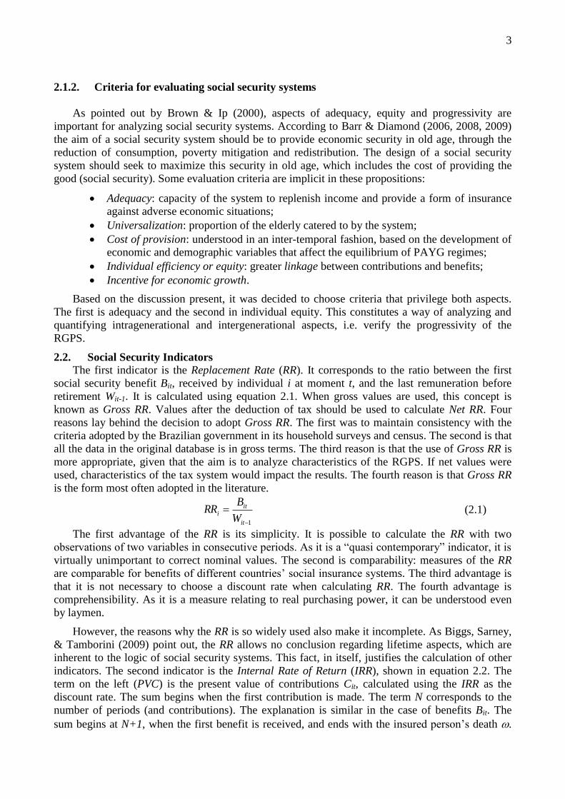
2.1.2. Criteria for evaluating social security systems

As pointed out by Brown & Ip (2000), aspects of adequacy, equity and progressivity are

important for analyzing social security systems. According to Barr & Diamond (2006, 2008, 2009)

the aim of a social security system should be to provide economic security in old age, through the

reduction of consumption, poverty mitigation and redistribution. The design of a social security

system should seek to maximize this security in old age, which includes the cost of providing the

good (social security). Some evaluation criteria are implicit in these propositions:

Adequacy: capacity of the system to replenish income and provide a form of insurance

against adverse economic situations;

Universalization: proportion of the elderly catered to by the system;

Cost of provision: understood in an inter-temporal fashion, based on the development of

economic and demographic variables that affect the equilibrium of PAYG regimes;

Individual efficiency or equity: greater linkage between contributions and benefits;

Incentive for economic growth.

Based on the discussion present, it was decided to choose criteria that privilege both aspects.

The first is adequacy and the second in individual equity. This constitutes a way of analyzing and

quantifying intragenerational and intergenerational aspects, i.e. verify the progressivity of the

RGPS.

2.2. Social Security Indicators

The first indicator is the Replacement Rate (RR). It corresponds to the ratio between the first

social security benefit Bit, received by individual i at moment t, and the last remuneration before

retirement Wit-1. It is calculated using equation 2.1. When gross values are used, this concept is

known as Gross RR. Values after the deduction of tax should be used to calculate Net RR. Four

reasons lay behind the decision to adopt Gross RR. The first was to maintain consistency with the

criteria adopted by the Brazilian government in its household surveys and census. The second is that

all the data in the original database is in gross terms. The third reason is that the use of Gross RR is

more appropriate, given that the aim is to analyze characteristics of the RGPS. If net values were

used, characteristics of the tax system would impact the results. The fourth reason is that Gross RR

is the form most often adopted in the literature.

1

it

iti

W

BRR (2.1)

The first advantage of the RR is its simplicity. It is possible to calculate the RR with two

observations of two variables in consecutive periods. As it is a “quasi contemporary” indicator, it is

virtually unimportant to correct nominal values. The second is comparability: measures of the RR

are comparable for benefits of different countries’ social insurance systems. The third advantage is

that it is not necessary to choose a discount rate when calculating RR. The fourth advantage is

comprehensibility. As it is a measure relating to real purchasing power, it can be understood even

by laymen.

However, the reasons why the RR is so widely used also make it incomplete. As Biggs, Sarney,

& Tamborini (2009) point out, the RR allows no conclusion regarding lifetime aspects, which are

inherent to the logic of social security systems. This fact, in itself, justifies the calculation of other

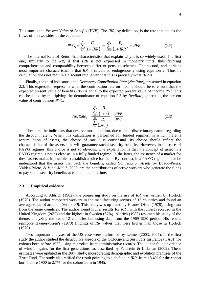
indicators. The second indicator is the Internal Rate of Return (IRR), shown in equation 2.2. The

term on the left (PVC) is the present value of contributions Cit, calculated using the IRR as the

discount rate. The sum begins when the first contribution is made. The term N corresponds to the

number of periods (and contributions). The explanation is similar in the case of benefits Bit. The

sum begins at N+1, when the first benefit is received, and ends with the insured person’s death .

4

This sum is the Present Value of Benefits (PVB). The IRR, by definition, is the rate that equals the

flows of the two sides of the equation.

i

Ntt

itN

tt

iti PVB

IRR

B

IRR

CPVC

11 11 (2.2)

The Internal Rate of Return has characteristics that explain why it is so widely used. The first

one, similarly to the RR, is that IRR is not expressed in monetary units, thus favoring

comprehension and comparability between different pension schemes. The second, and perhaps

most important characteristic, is that RR is calculated endogenously using equation 2. Thus its

calculation does not require a discount rate, given that this is precisely what IRR is.

Finally, the third indicator is the Necessary Contribution Rate (NecRate), presented in equation

2.3. This expression represents what the contribution rate on income should be to ensure that the

expected present value of benefits PVB is equal to the expected present value of income PVI. This

can be noted by multiplying the denominator of equation 2.3 by NecRate, generating the present

value of contributions PVC.

PVI

PVB

r

R

r

B

NecRateN

tt

it

Ntt

it

i

1

1

1

1

(2.3)

These are the indicators that deserve most attention, due to their discretionary nature regarding

the discount rate r. When this calculation is performed for funded regimes, in which there is

accumulation of assets, the choice of rate r is consensual. Its choice should reflect the

characteristics of the assets that will guarantee social security benefits. However, in the case of

PAYG regimes, this choice is not so obvious. One explanation is that the concept of asset in a

PAYG regime is not as clear as in a fully funded regime. In the latter, the existence of a market for

these assets makes it possible to establish a price for them. By contrast, in a PAYG regime, it can be

understood that the assets that back the benefits, called Contribution Assets by Boado-Penas,

Valdés-Prieto, & Vidal-Meliá, 2008, are the contributions of active workers who generate the funds

to pay social security benefits at each moment in time.

2.3. Empirical evidence

According to Aldrich (1982), the pioneering study on the use of RR was written by Horlick

(1970). The author compared workers in the manufacturing sectors of 13 countries and found an

average value of around 40% for RR. This study was up-dated by Haanes-Olsen (1978), using data

from the same countries. The author found higher results for RR , with the lowest recorded in the

United Kingdom (26%) and the highest in Sweden (67%). Aldrich (1982) resumed his study of the

theme, analyzing the same 12 countries but using data from the 1969-1980 period. His results

reinforce Haanes-Olsen's (1978) findings of RR values that were higher than those in Horlick

(1970).

Two important analyses of the US case were performed by Leimer (2003, 2007). In the first

study the author studied the distributive aspects of the Old-Age and Survivors Insurance (OASI) for

cohorts born before 1922, using microdata from administrative records. The author found evidence

of windfall gains for the first generations, as described by Feldstein & Liebman (2002). These

estimates were updated in the 2007 study, incorporating demographic and evolution premises of the

Trust Fund. The study also ratified the result pointing to a decline in IRR, from 18.4% for the cohort

born before 1900 to 2.7% for the cohort born in 1945.

5

This pattern of results was similar to those reported by Hurd & Shoven (1985) for the cohort

born between 1905 and 1911. For married individuals, the reported IRRs were 8.4%, while Leimer

(2007) found IRRs close to 8.6%. Duggan, Gillingham, & Greenlees (1993) reinforced the Old-Age,

Survivors and Disability Insurance (OASDI) pro-progressivity results. Their study analyzed

individuals of four cohorts: 1895-1903, 1904-1910, 1911-1916 and 1917-1922. The average IRR

reported was 9.1%. The RRs of women were 2.5% higher than male RRs. The same occurred in the

case of non-whites and lower income workers. Finally, evidence was found of windfall gains for

older generations.

An important advance occurred in the literature when Garrett (1995) incorporated income-

differentiated mortality. In this case, the clear evidence of progressivity in OASDI (in the form of

higher IRRs for lower-income individuals) was questioned, given that higher IRRs were obtained by

middle-income workers. In the same year, Duggan, Greenlees, & Greenless (1995) also obtained

less conclusive results when using income-differentiated mortality rates. Brown (1998) also

incorporated the latter, when analyzing the OASDI and Canada/Quebec Pension Plans (C/QPP).

The author concluded that both systems were progressive but that the OASDI was more so.

An important series of contributions for Latin American countries was made by Forteza &

Ourens (2009, 2012) e Forteza et al. (2009). In the first study they calculated the IRRs and RRs of

11 countries. The authors found evidence of progressivity, as IRRs were higher for lower-income

contributors. Obviously this conclusion is not valid for countries with funded regimes, such as

Chile, Uruguay and Colombia. In general the RRs calculated were very high, attaining 100% in

more than half of these countries.

In Forteza et al. (2009) there was a methodological modification: the authors used

administrative records of Chile’s and Uruguay’s social security regimes. The study found very low

RRs in the latter country: around 35% for men and 11% for women. After incorporating the legal

changes introduced in 2008, these values increased to around 50% and 28%, respectively. Forteza

& Ourens (2012) resumed their analysis of the 11 countries of the 2009 study, once again using

representative individuals, but this time employing a simulation model. These outcomes

corroborates their previous conclusion that the regimes were progressive, given that IRRs were

higher for lower-income individuals.

In Brazil, Fernandes (1994) was probably the first study to examine this theme. This author

analyzed various cohorts, from 1930-1935 onwards. The hypothesis adopted in the stylized model is

that all people retired at 65 or 60. In the latter case, the male IRR of the first cohort was 1.98%,

while a negative rate of -0.01% was found for the 1985-1990 cohort. In the case of women, the

values found were 2.83% and 0.67%, respectively. These numbers reinforced the hypothesis of

windfall gains and progressivity

Afonso & Fernandes (2005) calculated IRRs for cohorts born after 1920, with disaggregation by

educational level and region of the country, using microdata from the Brazilian National Household

Surveys (PNAD) of 1976 and 1999. The PNADs are household surveys performed annually by the

Brazilian government. The average real IRR was 6.7% and the study also found evidence of

progressivity, given that average values for the Northeast region (the poorest in the country) were

more than 1.5 percentage points higher than in other regions. Analogously, the IRR of individuals

with a lower educational level was more than one percentage point above the average. A similar

result regarding income transfers was obtained by Reis & Turra (2011), which incorporated the

populations composition differentials and regional mortality differentials.

Giambiagi & Afonso (2009) focused on the RGPS’s Retirement by Length of Contribution,

using microdata from the 2007 PNAD. The authors found evidence of progressivity; the necessary

rates of women were higher than men’s. In nearly all the cases analyzed, the values are lower than

the effective rates (evidence of the existence of cross subsidies between RGPS benefits). When RRs

6

were analyzed the pattern of results is a little less clear; the values obtained by groups with higher

levels of education were around 12 percentage points lower than those with lower levels. Similar

results were also obtained by Penafieri & Afonso (2013).

The possible existence of cross subsidies in the RGPS was examined in Caetano (2006). The

author calculated the IRRs of various groups of contributors, divided according to sex, type of

benefit and the incidence of the social security factor. In the case of a man who entered the labor

market at the age of 18 and retired by length of contribution at 53, the IRR was 1.68%. For a woman

who retired after 30 years of contribution, the IRR was 2.51%. There was evidence of progressivity,

with the lowest IRR s found for male Retirement by Length of Contribution to which the factor was

applied and the highest for women who retired by age and received a minimum wage.

It is possible to draw four conclusions from the literature. The general consensus is that social

security systems are progressive. The second conclusion is that there is strong evidence of the

existence of windfall gains for the first generations with access to the social security system. The

third is that gains are different and decrease over time. Finally, there are intragenerational transfers

between individuals of the same cohort.

3. DATA AND METHODOLOGY

3.1. Construction of the initial database using the RGPS’s administrative records

This section describes the database construction process based on primary information sources.

The records are held in the database of the Social Security’s Technology and Information Company

(Dataprev), which is responsible for processing data from Brazil’s Ministry of Social Security. The

microdata is on a monthly basis and covers a 27-year period from January 1980 to December 2006.

There are two sets of data. The first is the File of Formal Employment and Remunerations, The

second set is called the File of Benefits and contains information subsequent to the moment

contributors begin to receive social security benefits.

3.1.1. Formal Employment and Remunerations

This database has a single identifier for each individual. The codification of educational level is

presented in Table 1. The Retirement Benefit variable informs whether or not the benefit is a

pension. The Formal Employment Competency variable is a dummy variable that informs whether

there is, in any particular month, a record of remuneration (and contribution) to the RGPS. The

variable has a value of 1 in a positive case and 0 if not. There are 324 occurrences, as this is the

result obtained by multiplying the 12 months of the year by the 27 years of the sample. Finally, the

Remuneration-Link variable shows the value of the remuneration of insured persons, in multiples of

the nominal minimum wage prevailing at the time, multiplied by 100. It is important to highlight

that in Brazil the minimum wage constitutes an important index for both remunerations and

benefits. The floor for retirement benefits is equal to 1 minimum wage and more than two thirds of

retirement benefits correspond to this amount.

Initially there are 5,000 individuals in each cohort, comprising those born in 1930, 1935, 1940,

1945, 1950, 1955 and 1960, out of a total of 34,998 insured persons, because there was a problem

with two records of the 1930 cohort. There is a slight male predominance (53.2%) in the sample. As

there are many categories and the number of contributors per category is very small (considering

that more than 60% comprise category 0), it was decided to join four Educational Groups in the

way described in Table 2. Thus, the results will be given using these four groups.

7

Table 1 – Distribution of Educational Level by Category

Category Description Number %

0 No information 21,425 61.22

1 Illiterate 1,831 5.23

2 Incomplete primary 3,438 9.82

3 Complete primary 2,752 7.86

4 Incomplete gymnasium 1,359 3.88

5 Complete gymnasium 1,214 3.47

6 Incomplete high school 418 1.19

7 Complete high school 1,399 4.00

8 Incomplete higher education 219 0.63

9 Graduate 943 2.69

Total 34,998 100.00

Source: Tabulations Author’s calculation based on Dataprev administrative records

Table 2 – Educational Groups

Educational Group Educational Level (category)

0 0

1 1, 2, 3 e 4

2 5, 6 e 7

3 8 e 9

Source: Author’s calculation

3.1.2. Benefits

The structure of the File of Benefits database is similar to the File of Formal Employment and

Remunerations database It contains information on the type of benefit according to the Ministry of

Social Security’s classification of Benefits Provided on a Regular Monthly Basis, the date when the

benefit begins (DBB), the date when the benefit ends (DEB) and whether the benefit is a Survivor’s

Benefit. The RMI variable denotes the value of the first payment of the benefit in multiples of the

prevailing nominal minimum wage. However, unlike the procedure adopted in the case of

remunerations, the Benefits database contains only the value of the first benefit paid. Using a single

identifier, the components of this database are identified and attributed to the records of the File of

Formal Employment and Remunerations. In the case of benefits, records are only kept for

individuals who, during the period analyzed (1980 to 2006), were already beneficiaries. This is why

these databases are smaller than the Formal Employment and Remunerations databases, as can be

seen in Table 3. The remunerations database contains records for 34,998 individuals, compared to

only 22,916 individuals in the benefits database. And only 5,270 of this total are Retirement

Benefits by Age and 2,107 by Length of Contribution.

Table 3 – Distribution of Beneficiaries by Year of Birth Year of birth Number %

1930 3,319 14.48

1935 4,037 17.62

1940 3,990 17.41

1945 3,928 17.14

1950 3,284 14.33

1955 2,368 10.33

1960 1,990 8.68

Total 22,916 100.00

Source: Dataprev document sent to the author

8

The following stage consisted of building a single database for contributions and benefits for

individuals of all cohorts. Only two types of benefits were kept in the database: Retirement Benefits

by Length of Contribution (RBLC), and Retirement Benefits by Age (RBA). There are two reasons

for this choice. The first is that, of all the benefits paid by the Brazilian pension schem, these are the

types that closely relate benefits and contributions. The second reason is that the international

literature deals basically with programmable benefits. It was decided to exclude all survivors’

benefits from the databases, the main reason being that it is impossible to identify these survivor’s

benefits based on the benefit they are derived from.

3.2. Calculation of real values and contributions

After creating the initial database and performing the procedures described above, the next step

was to calculate the social security contributions made by insured persons, as the original database

did not contain this information. It is important to remember that the values of individuals’ income

Rem and benefits RMI are expressed in multiples of each month’s nominal minimum wage MW,

multiplied by 100. Thus, first of all, the Nominal Income and Benefit values of each insured person

i were calculated for each month t.

This was followed by calculating the social security contribution of each worker i in month t

according to employee and employer contribution rates. To achieve this, a close examination was

made of Brazilian social security legislation in order to find the contribution rates prevailing

between January 1980 and December 2006. It was found that, during these 27 years, 96 changes

had been made in rates and contribution ranges and limits. Changes occurred more frequently

during the period of hyperinflation and great economic instability between 1986 and 1994.

After calculating the nominal values of contributions these values were converted into constant

December 2006 Brazilian real (BRL) terms. The calculations were performed using the same

indicator used by the Ministry of Social Security, the National Consumer Price Index (INPC)

calculated by the government. In the case of values prior to the change in the currency carried out in

July 1994 as part of the Real Plan, the study adopted the methodology used by IPEA (a research

institute linked to the government) for the nominal minimum wage series. The penultimate stage of

the empirical procedure consisted of imputing the values of the 13th annual portion of income and

benefits, based on December of each year. This was performed because all formal Brazilian workers

and social security beneficiaries receive an extra payment during the last month of the year. Finally,

in order to make the results clearer for readers, all monetary values were converted into the average

exchange rate (2.15 BRL/US$) prevailing in December 2006.

3.3. Imputation of values for unobserved periods

After computing the real values of all variables, the next stage was to impute the data for all

unobserved periods, ie the years before 1982 and after 2006. The initial data covered a period of 25

years (already including the exclusion of the 1980 and 1981 data), which is relatively short given

the span of a life cycle. Thus, it was necessary to add extra years for the pre-1982 and post-2006

periods to the original database. The values of monetary variables (income, contributions and

benefits) and other observable characteristics were subsequently imputed during these periods. The

strategy adopted was divided into two parts. An empty database, beginning in 1944, was created for

the pre-1982 period and filled with each individual’s invariable information (identifier, type of

benefit, educational level), followed by monetary variables. The most important are income and

contributions and, implicitly, the contribution densities. We imputed for each year t (t<1982), for

each individual i with a vector of characteristics X, the same values of income and contributions that

individuals with this same vector of characteristics X show for the years between 1982 and 2006.

Considering the variables available and the fixed characteristics of each individual i of the sample,

X was defined according to equation 3.1

9

Group lEducationa Benefit, of Type Sex,Age,XX ii (3.1)

In the case of the second part – the period after 2006 – the procedure is a good deal simpler,

given that the workers should already have the benefit. Thus, mimicking the Ministry of Social

Security’s procedure of maintaining the real value of benefits, the last real value effectively

observed was replicated for subsequent years.

An original by-product for the Brazilian case was the calculation of the Contribution Density

CD for the period observed (1982-2006), as presented in equation 3.2. This is an indicator of the

relation between the number of social security contributions effectively made by each individual i

and the maximum possible number N of contributions that would have been made if the individual

had remained during the whole period in the formal labor market or had not had periods of

unemployment. By construction, the value of CDP for each insured person must lie in the [0,1]

range. The incorporation of Contribution Density constitutes an important difference of this article

in relation to studies which use representative individuals or cross-section data, such as the

Household Survey (PNAD). Particularly in this second case, as information is not available for

individuals’ entire active lives, authors usually consider that their contribution status remains the

same throughout life. This implicitly means adopting the hypothesis of a contribution density equal

to 1, which certainly does not occur, given periods of unemployment or informality.

N

ContribN

CD

N

t

it

i

1

º

(3.2)

The value of CD was calculated for the whole sample during the period for which primary

income values are available (1982-2006). This data showed that contribution density is equal to

0.6975. This very low value (under 70%) constitutes evidence of the importance of incorporating

contribution density, which reveals the high level of informal labor in the Brazilian labor market.

The last stage consisted of imputing life expectancies, using Brazilian abbreviated mortality

tables by sex, cohort and five-year period [from the Economic Commission for Latin America and

the Caribbean (ECLAC)]. These tables were covered the five-year periods 1960-1965, 1955-1960

and 1950-1955. As the database contains individuals who were born as from 1930, life expectancies

were extrapolated for each age in the case of older cohorts. Given the lack of more precise

information, a form of “aggravating” the mortality tables was adopted, with a consequent reduction

in life expectancies. This consisted of adopting a reduction for each age group that corresponded to

the average of the ratio found for the tables for which there was information. For example, suppose

that from 1955-1960 to 1960-1965 life expectancies for a certain age increased from 18 to 20 years;

and from 1950-1955 to 1955-1960 life expectancies for a certain age rose from 16 to 20. The

average increase was therefore the average between 2/18 and 2/16.

3.4. Calculation of indicators, exclusion of observations and identification of outliers.

Due to its operational simplicity the Replacement Rate RR was the first indicator to be

calculated. Following the procedure adopted by various authors, the calculation was performed

using not only the last remuneration received immediately before the date of the first benefit (DFB),

but the 12-month period prior to obtaining the benefit. The aim was prevent short-term fluctuations

form influencing the results.

It was not possible to calculate the RR for a significant number of beneficiaries because the

contribution period ended a long time before (more than a year) they began to receive the retirement

benefit. Apparently this puzzle is inherent to the characteristics of the database and the Brazilian

pension scheme and it was impossible to find a consistent explanation. It was decided to exclude all

records for which it was not possible to calculate the RR from the sample. Following this procedure,

10

the number of individuals fell from 7,325 to 1,733. 193 benefits classified as survivor’s benefits

were eliminated from the latter due to the reasons mentioned above.

The calculation of the IRR and NecRate indicators revealed some outliers, which were clearly

incompatible with the patterns and results expected for a social security system. The identification

of these patterns is linked to the values reported by the empirical literature, such as, for example,

Afonso & Fernandes (2005) and Giambiagi & Afonso (2009), for the Brazilian case and Forteza &

Ourens (2009). These outliers probably derive from two sources. The first is some kind of problem

with the Dataprev’s administrative records. The second are distortions in the data, especially during

the period of high inflation and successive economic plans between 1986 and 1994.

It was decided to adopt a procedure to identify and exclude the outliers using the results

calculated for RR, IRR and NecRate. Following Weber's (2010) recommendation, a blocked

adaptive computationally efficient outlier nominator (bacon) routine was used. This routine was

developed by Sylvain Weber and can be obtained at http://www.stata-journal.com/software/sj10-3.

The author provides evidence showing its advantages in relation to the hadimvo routine presented

by Hadi (1992) and Hadi (1994), given that it manages to identify a similar set of outliers, but with

computational gains. Using the bacon routine led to the elimination of 95 of the 1,540 records that

comprised the sample. This approximately 6.2% loss can be deemed acceptable given the aims of

the study and the type of microdata used. The results reported below were obtained for the 1,445

remaining records, which comprise what was called the Full Sample.

4. RESULTS

After describing the procedures involved in building the database in the previous section, this

section presents the results of the Social Security indicators. All values are presented for the Full

Sample and for the following categories of analysis: sex, type of benefit, cohort, educational group

and income quartile. However, this is preceded by a presentation of the most important descriptive

statistics. Table 4 shows the number of individuals in the Full Sample by year of birth and sex. The

procedure used to divide the data in the database explains why only 14 individuals were born in

1960. In 2006, the most recent year of the sample, the individuals who were born in 1960 were 46

years old and too young to receive a Retirement Benefit by Length of Contribution. By contrast, the

explanation for the small number of individuals born in 1930 (89 people) is the opposite. The life

expectancy of older cohorts is considerably lower than younger ones.

With the exception of the 1930 and 1950, the proportion of women in the sample is relatively

stable. The 1940, 1945 and 1950 cohorts are the most numerous in the sample and account for more

than 64% of the total. Table 5 presents the cross tabulation between the two types of benefits and

sex. Nearly 62% of the benefits in the sample are RBAs and the remainder RBLCs. However, there

is an important difference: men represent the majority of the RBLCs (78.7%) and women are the

majority group (62.1%) in RBAs. This male predominance was to be expected given that in the past

there were far fewer women in the labor market, especially the formal one. This is reflected later in

the smaller number of programmable benefits.

Table 6 shows that more than 40% of beneficiaries were in Educational Group 1. The number

of components of groups 2 and 3, which encompass individuals with higher educational levels, was

much lower. The only noteworthy difference between men and women is related to their

participation in groups 0 and 1. There are no microdata on educational levels for nearly a third of

the sample. This problem is more serious in the case of women’s administrative records, where

nearly 43% do not have this information. The information regarding educational levels is obtained

when workers join the RGPS, or some other situation which justified updating personal details. As

this information is not essential for the Ministry of Social Security, its reliability is probably not

very high, given that any additional collection effort would serve no useful purpose. This hypothesis

is corroborated by the fact that there is no data for this variable for more than 32% of individuals.

11

Table 4 – Number of Individuals by Year of Birth and Sex

Year Female Male Total

Number % Number % Number

1930 57 64.04 32 35.96 89

1935 137 43.49 178 56.51 315

1940 150 42.02 207 57.98 357

1945 139 42.77 186 57.23 325

1950 66 26.61 182 72.39 248

1955 39 40.21 58 59.79 97

1960 6 42.86 8 57.14 14

Total 594 41.11 851 58.89 1,445

Source: Author’s calculation based on Dataprev administrative records.

Table 5 – Number of Beneficiaries by Type of Benefit and Sex

Type Female Male Total

Number % Number % Number %

RBA 369 62.12 181 37.88 550 38.06

RBLC 225 21.27 670 78.73 895 61.94

Total 594 41.11 851 58.89 1,445 100.00


Table 6 – Number of Beneficiaries by Sex and Educational Group

Sex Group 0 Group 1 Group 2 Group 3 Total

Number % Number % Number % Number % Number

Female 254 42.76 190 31.99 103 17.34 47 7.91 594

Male 215 25.26 401 47.12 161 18.92 74 8.70 851

Total 469 32.46 591 40.90 264 18.27 121 8.37 1,445


Table 7 – Number of Beneficiaries by Year of Birth and Educational Group

Year Group 0 Group 1 Group 2 Group 3 Total

Number % Number % Number Number % Number %

1930 72 80.90 16 17.98 1 1.12 0 0.00 89

1935 176 55.87 101 32.06 24 7.62 14 4.44 315

1940 121 33.89 157 43.98 58 16.25 21 5.88 357

1945 70 21.54 161 49.54 63 19.38 31 9.54 325

1950 24 9.68 115 46.37 76 30.65 33 13.31 248

1955 6 6.19 34 35.05 37 38.14 20 20.62 97

1960 0 0.00 7 50.00 5 35.71 2 14.29 14

Total 469 32.46 591 40.90 264 18.27 121 8.37 1,445


Finally table 8 shows another important difference between sexes regarding the number of

beneficiaries by income. There are far more men in the higher income quartiles, reflecting that fact

that men’s remuneration is greater than women’s. This inequality is important in explaining the

differences found between the social security indicators of both sexes.

12

Table 8 – Number of Beneficiaries by Sex and Income Quartile

Sex Quartile 1 Quartile 2 Quartile 3 Quartile 4 Total


Women 232 39.06 183 30.81 99 16.67 80 13.47 594

Men 96 11.28 186 21.86 268 31.49 301 35.37 851

Total 328 22.70 369 25.54 367 25.40 381 26.37 1,445


The differences in remuneration can also be seen in the evolution of income from work during

active life, whether in the case of the Full Sample or the categories of analysis presented above. Due

to the sample’s small size (a problem worsened when the information is segregated by category), all

the graphs are constructed according to five-year age groups.

Graph 1 shows average income during the life cycle for the Full Sample. The curve is clearly

concave with the maximum located before 40 years (which is surprisingly early), then declining and

remaining practically stable from 55 to 59 onwards. The shape of this graph’s income curve can be

better understood by a comparison with Graph 2, which presents average income by Educational

Group. As expected, Group 3 (higher education) commands a substantial wage premium in relation

to Groups 2 (secondary education) and 1 (primary education). It is reasonable to infer that the

curve’s ascending shape for lower ages can be partially explained by the behavior of the income of

the group with the higher level of education (although it should be noted that the income of the

other groups also has concavity, but this is not so visible due to the scale of the graph), as can be

seen in Graph 2. The ascending shape for higher ages does not seem to have a significant overall

effect, given the small number of individuals in this group. Thus, the effect of Groups 1 and 2 is to a

certain extent superimposed. The behavior of Group 0 (for which there is no information on

education) is very similar to that of Groups 1 and 2, which seems to show that the lack of

information regarding levels of education is greater for the two lower educational groups. The

income profile is quite different from the one presented by Giambiagi & Afonso (2009, p. 162-164),

showing that using cross-section data can generate different results from those obtained by using

administrative records, which was the procedure adopted in the present study.

Graph 1 – Mean Monthly Income by Age Group


0

200

400

600

800

1,000

1,200

1,400

25-29 30-34 35-39 40-44 45-49 50-54 55-59 60-64 65-69 70-74

Mea

n M

on

thly

In

com

e (U

S$

)

Age Group

13

Graph 2 - Mean Monthly Income by Age Group and Educational Group

Source: Author’s calculation based on Dataprev administrative records Dataprev.

Graph 3 shows average income by age, disaggregated by sex. Male income is higher for most

ages, a phenomenon which must be linked to differences in educational levels. Graph 4 shows the

income of individuals who retired by length of contribution and of those who obtained the benefit

by age. There are clear differences, with higher earnings for the first group. This result is consistent

with stylized facts regarding social security in Brazil, in which individuals who obtain the RBLC

have a higher income and retire earlier, in addition to receiving a higher benefit. This argument can

be visualized in Table 9, which shows average levels of income and benefits, by income quartile,

for the Full Sample. It also presents the relation between benefits and income which declines

monotonically with the increase in income. This indicator provides yet more evidence that the

RGPS - for the benefits under analysis – is progressive. A similar analysis can be performed using

Table 10, in which values are segregated by type of benefit.

Graph 3 - Mean Monthly Income by Age Group and Sex


0

500

1,000

1,500

2,000

2,500

3,000

3,500

4,000

25-29 30-34 35-39 40-44 45-49 50-54 55-59 60-64 65-69 70-74

Mea

n M

on

thly

In

com

e (U

S$

)

Age Group

Educational Group 0 Educational Group 1

Educational Group 2 Educational Group 3

0

200

400

600

800

1,000

1,200

1,400

25-29 30-34 35-39 40-44 45-49 50-54 55-59 60-64 65-69 70-74

Mea

n M

on

thly

In

com

e (U

S$

)

Age Group

Men Women

14

Graph 4 - Mean Monthly Income by Age Group and Type of Benefit

Source: Author’s calculation based on Dataprev administrative records..

Table 9 – Average Value of Benefits and Income by Income Quartile

Quartile 1 Quartile 2 Quartile 3 Quartile 4 Full Sample

Average benefit (US$) 178.10 346.97 609.30 956.39 535.95

Average Income (US$) 134.32 270.08 562.03 2,109.82 798.50

Benefit/Income (%) 132.59 128.47 108.41 45.33 67.12

Number 328 369 367 381 1,445


Table 10 – Average Value of Benefits and Income by Type of Benefit

RBA RBLC Full Sample

Average Benefit (US$) 298.33 681.98 535.95

Average Income (US$) 324.54 1,089.75 798.50

Benefit/Income (%) 91.92 62.58 67.12

Número 550 895 1,445


4.1. Replacement Rate (RR)

This section presents the results obtained for the Replacement Rate RR. It reports the values for

the Full Sample and by category of analysis. The average RR for the 1,445 individuals in the Full

Sample was a high 82.52%. Table 11 reports these values and shows a reduction in the RR over

time for younger cohorts. This decrease may be understood as evidence of the existence of windfall

gains associated with the expansion of the social security system in Brazil. This is similar to what

Leimer (2003, 2007) and Duggan et al. (1993) verified in the USA.

Table 12 presents values disaggregated by sex, with female RR around 10 percentage points

higher than male RR. This difference is perhaps due to the characteristics of insured workers’

average income and the existence of a ceiling for the value of benefits. This line of reasoning is

corroborated by the results of Table 13, which shows that the RRs of RBAs are more than 20

percentage points higher than those of RBLCs. The results of Table 14 show that, with the

exception of Group 0, the educational values are inversely related to these values. RR values are

reported for income quartiles in Table 15, with higher incomes associated with lower RRs.

0

200

400

600

800

1,000

1,200

1,400

25-29 30-34 35-39 40-44 45-49 50-54 55-59 60-64 65-69 70-74

Mea

n M

on

thly

In

com

e (U

S$)

Age Group

Retirement by age Retirement by length of contribution

15

Table 11 – Replacement Rate (RR) by Cohort Cohort N Average (%) Standard-deviation Minimum Maximum

1930 89 95.14 32.74 10.42 230.16

1935 315 86.37 36.20 7.16 246.17

1940 357 87.71 33.68 6.25 241.16

1945 325 84.23 36.53 5.86 266.96

1950 248 73.35 37.13 8.64 261.07

1955 97 60.45 30.11 10.98 165.60

1960 14 58.71 26.08 24.51 105.62

Full Sample 1,445 82.52 36.12 5.86 266.96


Table 12 – Replacement Rate (RR) by Sex Sex N Average (%) Standard-deviation Minimum Maximum

Femle 594 88.32 32.54 5.86 246.17

Male 851 78.46 37.92 6.18 266.96

Full Sample 1,445 82.52 36.12 5.86 266.96

Source: Author’s calculation based on Dataprev administration records.

Table 13 – Replacement Rate (RR) by Type of Benefit Type of benefit N Average (%) Standard-deviation Minimum Maximum

RBA 550 96.27 30.04 7.16 241.16

RBLC 895 74.07 36.95 5.86 266.96

Full Sample 1,445 82.52 36.12 5.86 266.96

Source: Author’s calculations based on Dataprev administrative records.

Table 14 – Replacement Rate (RR) by Educational Group Educational Group N Average (%) Standard-deviation Minimum Maximum

Educational Group 0 469 86.63 33.63 5.86 231.41




Full Sample 1,445 82.52 36.12 5.86 266.96


Table 15 – Replacement Rate (RR) by Income Income quartile N Average (%) Standard-deviation Minimum Maximum

Quartile 1 328 101.42 27.81 17.72 246.17

Quartile 2 369 89.94 33.96 7.16 241.16

Quartile 3 367 86.54 32.19 12.40 266.96

Quartile 4 381 55.18 32.41 5.86 243.26

Full Sample 1,445 82.52 36.12 5.86 266.96

Source: Author’s calculation, based on Dataprev administrative records.

This first set of results should be analyzed together. It is noteworthy that the average values

found are higher than in other studies, For example, Giambiagi & Afonso ( 2009) and Penafieri &

Afonso (2013). These differences may be a sign that the RGPS is more generous than pension

regimes in other countries. The results show that the first generations were benefited from social

security. In other words, they provide support for the thesis of the existence of intergenerational

transfers and especially the existence of windfall gains in the RGPS, as shown by Feldstein &

Liebman (2002) and Feldstein (2005a, 2005b). The second aspect refers to the existence of

intragenerational transfers. Different RR values were found for groups separated according to sex,

type of benefit, educational level and income. Higher values were found for RBAs in relation to

RBLCs, for women in relation to men, for individuals with lower levels of education in relation to

16

those with higher educational levels and for the first income quartiles in relation to the last quartiles.

The lower the income of the insured worker, the higher his or her RR.

4.2. Internal Rate of Return (IRR)

The second Social Security Indicator calculated is the Internal Rate of Return (IRR). A real

average value of 5.32% per year was obtained for the Full Sample, which is also considerably

higher than the patterns found in the literature. The data by cohort show a large increase in the

values for younger cohorts (Table 16), differently from what was verified in the case of the RR, in

which higher values were found for older cohorts. A familiar pattern had been found by Afonso and

Fernandes (2005), albeit without disaggregating private and public sector workers. The average

values found here (5.32%) were lower than those verified in the study cited (6.7%). However, they

are much higher, on average than the values calculated by Caetano (2006) and Penafieri & Afonso

(2013). Similarly to the case of the RR, the average IRR for men is significantly lower than

women’s, as shown in Table 17.

Table 16 – Internal Rate of Return (IRR) by Cohort (real per year) Cohort N Average(%) Standard-deviation Minimum Maximum

1930 89 4.34 2.67 -3.12 14.76

1935 315 4.75 3.84 -10.56 21.08

1940 357 5.90 4.95 -3.90 21.75

1945 325 5.53 4.77 -1.84 25.97

1950 248 4.82 3.28 -3.99 22.27

1955 97 6.22 3.53 -0.90 15.74

1960 14 7.70 4.83 1.72 16.94

Full sample 1,445 5.32 4.25 -10.56 25.97


Table 17 – Internal Rate of Return (IRR) by Sex (real per year) Sex N Average (%) Standard-deviation Minimum Maximum

Female 594 6.33 4.64 -10.56 25.97

Male 851 4.62 3.79 -4.09 21.54

Full Sample 1,445 5.32 4.25 -10.56 25.97


The results separated by Educational Group, reported in Table 18, seem to indicate that insured

workers with a low educational level have a much higher IRR than those with a secondary or

university level of education. In Table 19, disaggregation by type of benefit shows that RBAs are

around 4 percentage points higher than RBLCs. The data by income quartile show the same pattern:

higher values are associated with lower income groups, with a great similarity between the second

and third quartiles, but with a notable difference between the extremes of the distribution. These

high results reinforce the evidence of the RGPS’s progressivity.

Table 18 – Internal Rate of Return (IRR) by Educational Group (real per year) Educational Group N Average(%) Standard-deviation Minimum Maximum

Educational Group 0 469 6.54 4.72 -10.56 25.97




Full Sample 1,445 5.32 4.25 -10.56 25.97


17

Table 19 – Internal Rate of Return (IRR) by Type of Benefit (real % per year) Type of benefit N Average(%) Standard-deviation Minimum Maximum

RBA 550 7.86 4.47 -10.56 25.97

RBLC 895 3.77 3.24 -4.09 22.27

Full Sample 1,445 5.32 4.25 -10.56 25.97


Table 20 – Internal Rate of Return (IRR) by Income Quartile (real % per year) Income quartile N Average (%) Standard-deviation Minimum Maximum

Quartile 1 328 6.66 5.04 -3.12 22.10

Quartile 2 369 5.59 4.20 -4.09 20.51

Quartile 3 367 5.39 4.07 -3.99 25.97

Quartile 4 381 3.85 3.13 -10.56 18.40

Full Sample 1,445 5.32 4.25 -10.56 25.97


4.3. Necessary Rate (NecRate)

The Necessary Rate is the rate that should be charged on insured persons’ incomes to ensure

that the present value of their contributions is equal to the present value of the benefits. The values

found are very high, with the average value exceeding 50%. The value of the NecRate increases as

from the 1930 cohort until reaching its highest value for the 1940 cohort, in which the maximum

value surpasses 55%. Lower values were found for the following generations with the value for the

1960 generation declining to 43% (see Table 21). Table 22 shows that the female rate should be

around 58% to balance contributions and benefits, which is 12 percentage points higher than the

values found for men. Similarly to what was verified in the case of the IRR (and the opposite of

what was verified for RR), the values decline monotonically for higher educational levels, with a

substantial difference between the values of Educational Groups 1 and 3. A similar behavior was

verified in the case of types of benefits, with much higher values for RBAs than for RBLCs (Table

23). Finally, when the dimension of analysis is income, the highest values (nearly 53%) are found

for lower income individuals. As income increases, the value of the rate decreases until reaching an

average value of just over 40% for the highest income quartile.

Table 21 – Necessary Rate (NecRate) by Cohort Cohort N Average(%) Standard-deviation Minimum Maximum

1930 89 49.69 27.72 3.20 136.42

1935 315 52.98 32.66 1.65 184.32

1940 357 55.87 35.84 4.87 198.75

1945 325 48.68 28.66 5.40 166.35

1950 248 45.52 27.61 7.07 204.77

1955 97 43.73 23.23 9.16 124.92

1960 14 43.16 26.24 15.67 96.49

Full Sample 1,445 50.53 31.13 1.65 204.77


Table 22 – Necessary Rate (NecRate) by Sex Sex N Average (%) Standard-deviation Minimum Maximum

Female 594 57.59 33.68 1.65 204.77

Male 851 45.60 28.21 3.20 198.75

Full Sample 1,445 50.53 31.13 1.65 204.77


18

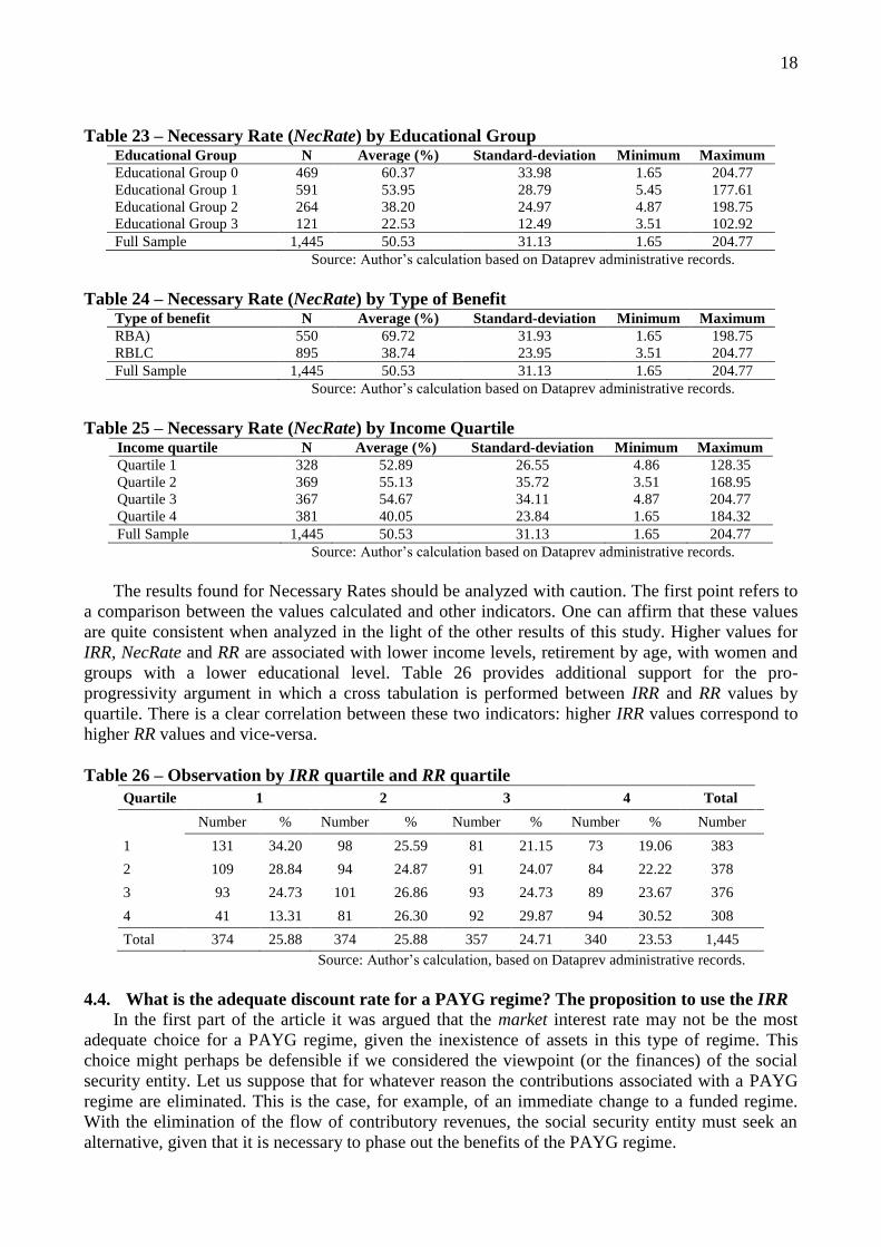
Table 23 – Necessary Rate (NecRate) by Educational Group Educational Group N Average (%) Standard-deviation Minimum Maximum





Full Sample 1,445 50.53 31.13 1.65 204.77


Table 24 – Necessary Rate (NecRate) by Type of Benefit Type of benefit N Average (%) Standard-deviation Minimum Maximum

RBA) 550 69.72 31.93 1.65 198.75

RBLC 895 38.74 23.95 3.51 204.77

Full Sample 1,445 50.53 31.13 1.65 204.77


Table 25 – Necessary Rate (NecRate) by Income Quartile Income quartile N Average (%) Standard-deviation Minimum Maximum

Quartile 1 328 52.89 26.55 4.86 128.35

Quartile 2 369 55.13 35.72 3.51 168.95

Quartile 3 367 54.67 34.11 4.87 204.77

Quartile 4 381 40.05 23.84 1.65 184.32

Full Sample 1,445 50.53 31.13 1.65 204.77


The results found for Necessary Rates should be analyzed with caution. The first point refers to

a comparison between the values calculated and other indicators. One can affirm that these values

are quite consistent when analyzed in the light of the other results of this study. Higher values for

IRR, NecRate and RR are associated with lower income levels, retirement by age, with women and

groups with a lower educational level. Table 26 provides additional support for the pro-

progressivity argument in which a cross tabulation is performed between IRR and RR values by

quartile. There is a clear correlation between these two indicators: higher IRR values correspond to

higher RR values and vice-versa.

Table 26 – Observation by IRR quartile and RR quartile

Quartile 1 2 3 4 Total


1 131 34.20 98 25.59 81 21.15 73 19.06 383

2 109 28.84 94 24.87 91 24.07 84 22.22 378

3 93 24.73 101 26.86 93 24.73 89 23.67 376

4 41 13.31 81 26.30 92 29.87 94 30.52 308

Total 374 25.88 374 25.88 357 24.71 340 23.53 1,445

Source: Author’s calculation, based on Dataprev administrative records.

4.4. What is the adequate discount rate for a PAYG regime? The proposition to use the IRR

In the first part of the article it was argued that the market interest rate may not be the most

adequate choice for a PAYG regime, given the inexistence of assets in this type of regime. This

choice might perhaps be defensible if we considered the viewpoint (or the finances) of the social

security entity. Let us suppose that for whatever reason the contributions associated with a PAYG

regime are eliminated. This is the case, for example, of an immediate change to a funded regime.

With the elimination of the flow of contributory revenues, the social security entity must seek an

alternative, given that it is necessary to phase out the benefits of the PAYG regime.

19

Eliminating the possibility of issuing money, the only remaining alternative is to issue bonds,

leading to an increase in the public debt and the payment of interest to the holders of these bonds.

Thus, the opportunity cost for the government, associated with the elimination of contributions, is

linked to the long-term interest rate on government bonds. To understand the problem in another

way it is worthwhile revisiting the concept of Contribution Asset, explored by Boado-Penas et al

(2008, p. 92-93), along with the Actuarial Balance Sheet of the social security regime. The authors’

approach is ingenious, given that, in the same study, they manage to bring together economic

principles associated with the PAYG regime and actuarial principles (the concern with the inter-

temporal solvency of the social security entity). In this case, calculating the assets of the system

means, in sort of a tautological method, calculating the value of social security liabilities.

This section proposes using the IRR to discount monetary values in a PAYG regime. This

choice can be better understood by shifting the focus from the social security entity to the

beneficiary. A pension scheme is a type of social contract involving government and workers. The

receipt of benefits depends on contributions. In other words, workers accept a reduction in their net

present incomes so that they can obtain future income. The relation between the flows of

contributions and benefits defines the IRR associated with their participation in the social security

system. Or, expressing this in a different way, the opportunity cost for workers of not contributing

to social security corresponds to not obtaining the IRR.

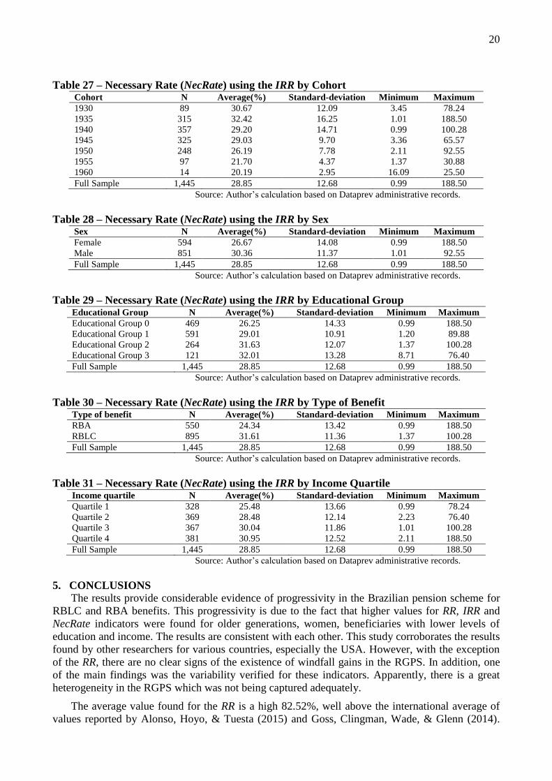
Based on this argument, this section redoes the calculation of the Necessary Rate, this time

using the value of the individual IRR, previously calculated for each beneficiary in the sample, as

the discount rate. Using the value of the IRR for each individual is justified by the fact that, as

shown above, it reflects each insured person’s opportunity cost. In a certain way, it is like using the

value of the biological interest rate inherent to a PAYG regime as a discount rate, an approach

presented for the first time in Samuelson's classic study(1958), albeit with heterogeneous agents and

with the generalization presented by Settergren & Mikula (2005, p. 124). Heterogeneity is based on

the different values obtained for Social Security Indicators, particularly the IRR, calculated for the

categories of analysis used here.

The average value of the NecRate is much closer for the average of individuals. There is also a

sharp reduction in the dispersion of values calculated, as the coefficient of variation falls from

around 0.62 para 0.44. The analysis of the results by categories reveals significant differences in

relation to the original values of NecRate calculated using a discount rate of 3% a year such as, for

example, in the case of the rate by sex. In the initial calculation, the average value of the NecRate

for women (men) was 57.59% (45.60%). Using the IRR, the values change, respectively, to 26.67%

and 30.36, i.e. the Necessary Rate for women is now lower than men’s. The explanation is that,

initially, the net present value of both sexes’ benefits was calculated using the same rate of 3%.

With the average IRR, the rate used for men increases to 4.62%, but increases even more for women

because the average IRR is 6.33. This increase affects benefits more than contributions, given that

the retirement benefits are more distant, thus leading to a greater reduction in their present value. Of

all the categories analyzed, the most radical change in results was seen in the type of benefit. The

new average value of NecRate for RBLCs (31.61%) is considerably lower than the value for RBAs

(24.34%). Once again the explanation is that, in the case of RBAs, the increase in the discount rate

is much more drastic than for RBLCs.

20

Table 27 – Necessary Rate (NecRate) using the IRR by Cohort Cohort N Average(%) Standard-deviation Minimum Maximum

1930 89 30.67 12.09 3.45 78.24

1935 315 32.42 16.25 1.01 188.50

1940 357 29.20 14.71 0.99 100.28

1945 325 29.03 9.70 3.36 65.57

1950 248 26.19 7.78 2.11 92.55

1955 97 21.70 4.37 1.37 30.88

1960 14 20.19 2.95 16.09 25.50

Full Sample 1,445 28.85 12.68 0.99 188.50


Table 28 – Necessary Rate (NecRate) using the IRR by Sex Sex N Average(%) Standard-deviation Minimum Maximum

Female 594 26.67 14.08 0.99 188.50

Male 851 30.36 11.37 1.01 92.55

Full Sample 1,445 28.85 12.68 0.99 188.50


Table 29 – Necessary Rate (NecRate) using the IRR by Educational Group Educational Group N Average(%) Standard-deviation Minimum Maximum





Full Sample 1,445 28.85 12.68 0.99 188.50


Table 30 – Necessary Rate (NecRate) using the IRR by Type of Benefit Type of benefit N Average(%) Standard-deviation Minimum Maximum

RBA 550 24.34 13.42 0.99 188.50

RBLC 895 31.61 11.36 1.37 100.28

Full Sample 1,445 28.85 12.68 0.99 188.50


Table 31 – Necessary Rate (NecRate) using the IRR by Income Quartile Income quartile N Average(%) Standard-deviation Minimum Maximum

Quartile 1 328 25.48 13.66 0.99 78.24

Quartile 2 369 28.48 12.14 2.23 76.40

Quartile 3 367 30.04 11.86 1.01 100.28

Quartile 4 381 30.95 12.52 2.11 188.50

Full Sample 1,445 28.85 12.68 0.99 188.50


5. CONCLUSIONS

The results provide considerable evidence of progressivity in the Brazilian pension scheme for

RBLC and RBA benefits. This progressivity is due to the fact that higher values for RR, IRR and

NecRate indicators were found for older generations, women, beneficiaries with lower levels of

education and income. The results are consistent with each other. This study corroborates the results

found by other researchers for various countries, especially the USA. However, with the exception

of the RR, there are no clear signs of the existence of windfall gains in the RGPS. In addition, one

of the main findings was the variability verified for these indicators. Apparently, there is a great

heterogeneity in the RGPS which was not being captured adequately.

The average value found for the RR is a high 82.52%, well above the international average of

values reported by Alonso, Hoyo, & Tuesta (2015) and Goss, Clingman, Wade, & Glenn (2014).

21

Evidence of progressivity was found for all categories of analysis. The values found were also much

higher than those found by other authors, such as Giambiagi & Afonso (2009) and Penafieri &

Afonso (2013). This seems to constitute an important difference in this study’s findings in relation

to studies that use representative groups of individuals. Similar conclusions are obtained based on

the results of the IRR. However, this indicator’s average real value of 5.32% is not that much higher

than the one found by other studies such as, for example, Clingman, Burkhalter, & Chaplain (2014).

The average value of over 50% found for NecRate is considerably higher than the level reported

in the literature. Although evidence of progressivity was also obtained for this indicator, it appears

to be weaker than in the case of the RR and the IRR. For example, there is a difference of only 12

percentage points between income quartiles. Very high values were also found, which is perhaps

due to low contribution densities, with an effective period of contribution that is much shorter than

the period during which benefits are received. It is possible that these values are the result of

rational arbitrage undertaken by contributors in face of lax benefit calculation rules and eligibility

conditions. It cannot be discarded that, mainly in the more distant past, there was a greater under-

declaration of income (and contributions) than during periods that were not part of the calculation

of the value of retirement benefits, which had a positive impact on the NecRate.

Based on these results, an additional exercise was performed related to a strand of the literature

which focuses on the analysis of solvency and measures of wealth associated with social security

systems. Part of this literature advocates, based on the concept of Contribution Asset (Boado-Penas

et al., 2008), that the risk-free rate of interest should be used as the discount rate in PAYG regimes.

It would be more appropriate to use the return obtained by contributors who take part in a PAYG

regime (Settergren; Mikula, 2005). The values of the NecRate were recalculated using the values of

each individual’s previously calculated IRR.

This change alters the results significantly. The values of NecRate are much lower for women

and beneficiaries with RA benefits, low educational levels and from the first income quartiles. This

occurs mainly because the benefits are discounted using much higher rates than those initially used.

The opposite occurs in the case of groups at the other extreme of the distribution. The interpretation

of the results is not immediate. It can be seen as a more adequate measure, from the individual point

of view, of the existence of distributive aspects, given the heterogeneity verified in the results of

previous sections.

One may consider that this study made an original contribution to the Brazilian literature on

social security. Its most important finding is that there is significant evidence of progressivity in the

General Social Security Regime (RGPS). Future research could use a similar methodology to

investigate risk benefits, a subject that has received little attention to date in Brazil.

ACKNOWLEDGMENTS

The author would like to thank Conselho Nacional de Desenvolvimento Tecnológico e Científico

(CNPq - Brazil) for funding this research - Edital MCT/CNPq 14/2010, Grant 473817/2010-1.

REFERENCES

Aaron, H. (1966): The Social Insurance Paradox. The Canadian Journal of Economics and Political

Science 32(3), 371–374.

Afonso, L. E., & Fernandes, R. (2005): Uma estimativa dos aspectos distributivos da previdência

social no Brasil. Revista Brasileira de Economia 59(3), 295–334.

22

Aldrich, J. (1982): The Earnings Replacement Rate of Old-Age Benefits in 12 Countries, 1969-80.

Social Security Bulletin 45(11), 3–11.

Alonso, J., Hoyo, C., & Tuesta, D. (2015): A model for the pension system in Mexico: diagnosis

and recommendations. Journal of Pension Economics and Finance 14(1), 76–112.

Andrews, D. (2008): A Review and Analysis of the Sustainability and Equity of Social Security

Adjustment Mechanisms. PhD Dissertation. University of Waterloo.

Barr, N., & Diamond, P. (2006): The Economics of Pensions. Oxford Review of Economic Policy

22(1), 15–39.

Barr, N., & Diamond, P. (2008): Reforming pensions: principles and policy choices, Oxford

University Press.

Barr, N., & Diamond, P. (2009): Reforming pensions: Principles, analytical errors and policy

directions. International Social Security Review, 62(2), 5–29.

Bertranou, F. M., & Sánchez, A. P. (2003): Características y determinantes de la densidad de

aportes a la Seguridad Social en la Argentina 1994-2001. In F. M. Bertranou, M. Bourquín, &

H. Pena (Eds.), Historias Laborales en la seguridad social. Buenos Aires: Ministerio de

Trabajo, Empleo y Seguridad Social.

Biggs, A. G., Sarney, M., & Tamborini, C. R. (2009): A progressivity index for Social Security

2009-01. Issue Paper. Washington, D.C.

Boado-Penas, M. del C., Valdés-Prieto, S., & Vidal-Meliá, C. (2008): The Actuarial Balance Sheet

for Pay-As-You-Go Finance: Solvency Indicators for Spain and Sweden. Fiscal Studies 29(1),

89–134.

Brown, R. L. (1998): Social Security: Regressive or Progressive? North American Actuarial

Journal 2(2), 27–28.

Brown, R. L. (2008): Optimal financing of social security pension schemes and its design:

competing views of social security pension design and its impact on financing and its design

its impact on financing. In Technical Seminar for Social Security Actuaries and Statisticians 3.

International Actuarial Association (IAA).

Brown, R. L., & Ip, J. (2000): Social Security — Adequacy, Equity, and Progressiveness. North

American Actuarial Journal 4(1), 1–17.

Bucheli, M., Forteza, A., & Rossi, I. (2008): Work histories and the access to contributory pensions:

the case of Uruguay. Journal of Pension Economics and Finance 9(3), 369–391.

Caetano, M. A.-R. (2006): Subsídios cruzados na previdência social brasileira 1211. Ipea.

Clingman, M., Burkhalter, K., & Chaplain, C. (2014): Internal real rates of return under the OASDI

program for hypothetical workers 2014.5. Baltimore.

Duggan, J. E., Gillingham, R., & Greenlees, J. S. (1993): Returns paid to early social security

cohorts. Contemporary Economic Policy 11(4), 1–13.

Duggan, J. E., Greenlees, J. S., & Greenless, J. S. (1995): Progressive Returns to Social Security?

An Answer from Social Security Records 9501. Washington, D.C.

Feldstein, M. (2005a): Rethinking social insurance. The American Economic Review 95(1), 1–24.

Feldstein, M. (2005b): Structural Reform of Social Security. Journal of Economic Perspectives

19(2), 33–55.

23

Feldstein, M., & Liebman, J. B. (2002): Social Security. In A. J. Auerbach & M. Feldstein (Eds.),

Handbook of Public Economics Vol. 4, 2245–2324. North-Holland.

Fernandes, F. (1994): Sistema previdenciário e desigualdades inter e intrageracionais no Brasil: o

papel da dinâmica demográfica. Previdência Em Dados 9(4), 5–36.

Forteza, A., Apella, I., Fajnzylber, E., Grushka, C., Rossi, I., & Sanroman, G. (2009): Work

Histories and Pension Entitlements in Argentina, Chile and Uruguay 0926. 1–78. World Bank

SP Discussion Paper.

Forteza, A., & Ourens, G. (2009): How much do Latin American pension programs promise to pay

back? 0927 1-62. World Bank SP Discussion Paper.

Forteza, A., & Ourens, G. (2012): Redistribution, insurance and incentives to work in Latin-

American pension programs. Journal of Pension Economics and Finance 11(03), 337–364.

Garrett, D. M. (1995): The effects of differential mortality rates on the progressivity of social

security. Economic Inquiry 33(3), 457–475.

Giambiagi, F., & Afonso, L. E. (2009): Cálculo da alíquota de contribuição previdenciária

atuarialmente equilibrada: uma aplicação ao caso brasileiro. Revista Brasileira de Economia

63(2), 153–179.

Goss, S., Clingman, M., Wade, A., & Glenn, K. (2014): Replacement rates for retirees: what makes

sense for planning and evaluation? 155,1-8. Social Security Administration.

Haanes-Olsen, L. (1978): Earnings-Replacement Rate of Old-Age Benefits, 1965-55, Selected

Countries. Social Security Bulletin 41(1), 3–14.

Hadi, A. S. (1992): Identifying multiple outliers in multivariate data. Journal of the Royal Statistical

Society. Series B (Methodological) 54(3), 761–771.

Hadi, A. S. (1994): A modification of a method for the detection of outliers in multivariate samples.

Journal of the Royal Statistical Society. Series B 56(2), 393–396.

Horlick, M. (1970): The earnings replacement rate of old-age benefits: an international comparison.

Social Security Bulletin 33(3), 3–16.

Hurd, M. D., & Shoven, J. B. (1985): The Distributional Impact of Social Security. In D. A. Wise

(Ed.), Pensions, Labor, and Individual Choice I, 193–222. NBER.

Leimer, D. R. (2003): Historical Redistribution Under the Social Security Old-Age and Survivors

Insurance Program 101 1-75. Social Security Administration.

Leimer, D. R. (2007): Cohort-Specific Measures of Lifetime Social Security Taxes and Benefits 110,

1-104. Social Security Administration.

Musgrave, R. A. (1985): A brief history of fiscal doctrine. In A. J. Auerbach & M. Feldstein (Eds.),

Handbook of public Economics 1, 1–59. Elsevier.

Penafieri, A. C., & Afonso, L. E. (2013): O impacto da mudança da regra de cálculo das

aposentadorias por tempo de contribuição do INSS: o fator previdenciário é atuarialmente

justo? Economia Aplicada 17(4), 667–694.

Reis, C. de B., & Turra, C. M. (2011): Desigualdade regional na distribuição dos recursos

previdenciários: uma análise das transferências intrageracionais e de período. In Anais do

XXXIX Encontro Nacional de Economia da Anpec 1-20). Anpec.

24

Reznik, G. L., Weaver, D. A., & Biggs, A. G. (2009): Social Security and Marginal Returns to

Work Near Retirement 2009-02, 1-20. Social Security Issue Paper. Social Security

Administration.

Samuelson, P. A. (1958): An Exact Consumption-Loan Model of Interest with or without the Social

Contrivance of Money. Journal of Political Economy 66(6), 467-482.

Schröder, C. (2012): Profitability of pension contributions – evidence from real-life employment

biographies. Journal of Pension Economics and Finance 11(03), 311–336.

Settergren, O., & Mikula, B. D. (2005): The rate of return of pay-as-you-go pension systems: a

more exact consumption-loan model of interest. Journal of Pension Economics and Finance

4(2), 115–138.

Shoven, J. B., & Slavov, S. N. (2012a): The Decision to Delay Social Security Benefits: Theory and

Evidence 17866, 1-49. NBER Working Paper.

Shoven, J. B., & Slavov, S. N. (2012b): When Does It Pay to Delay Social Security? The Impact of

Mortality, Interest Rates, and Program Rules 18210, 1-31. NBER Working Paper.

Weber, S. (2010): bacon: An effective way to detect outliers in multivariate data using Stata (and

Mata). Stata Journal 10(3), 331–338.

progressivity and distributive aspects of brazil's … and distributive aspects of...

Documents