programming language support for sensor networks
TRANSCRIPT

Programming Language Support for
Sensor Networks
Yu David Liu
The Johns Hopkins UniversityBaltimore, MD 21218, USA
1 Introduction
In this project, we design new language abstractions in better support of sensornetwork programming. Sensor network has received wide attention from bothacademia and industry in recent years. As a somewhat entertaining testament,a recent special issue of TIME magazine (“WHAT’S NEXT”, Fall 2003) has sin-gled out sensor network as one of the few technologies ready to bring revolutionto the high-tech world. The fast growth of sensor networks demands good sup-port for the design of sensor network applications. However, as a new computinginfrastructure, sensor network carries some traits strikingly different from tra-ditional networks, and they put forward new requirements and challenges in therealm of software design.
1.1 New Requirements
Our language is especially motivated by the following requirements distinctivein the design of sensor network applications:
First of all, sensor network applications are typically straightforward forintra-node data processing, but complicated for inter-node communication. Eachnode in a sensor network normally does not achieve a task alone; instead, theycollaborate via complicated communications to achieve ambitious goals. Towrite a sensor network application, it is vital for software developers to have aclear understanding of what kind of communications each piece of software isinvolved, which will help lead to less error-prone software development.
Second, sensor network nodes are energy and memory constrained. Sensornetwork nodes are typically wireless nodes powered by battery. Depending onapplications, they might be scattered in battlefields, inside volcanos, or lion-roaming prairies. Once deployed, it is usually hard to recharge or change battery.In terms of memory, a sensor network is typically composed of numerous nodes,and each node has to be installed with limited memory to keep the cost of thewhole network low.
1

Third, sensor networks are densely populated and in a typical communica-tion scenario, it is less important to ask the question “which physical node amI going to talk with?”, than the question “what kind of node am I going to talkwith?” In fact, for many sensor applications, software developers can not antic-ipate the final deployment and topology of the whole network at all, thereforeit is in many case unwise to hard-code applications like “communicating withnode with certain MAC address”.
1.2 Our Approach
In this project, we propose a programming language for sensor networks, to-gether with a lightweight design of a virtual machine on top of which the com-piled form of our programming language is interpreted. It has the followingnovel features to adapt to the need listed earlier:
Communication Interface In our language, each unit of software runningon a sensor network node is associated with a list of connectors, which servesas communication interface for the software unit. All communications involvedby the software unit is through the interface. Thus, simply by looking throughwhat connectors each software unit has, we can easily know how the unit com-municates with the outside, which is especially helpful for developing sensor net-work applications, where inter-node communications are complicated. In addi-tion, since inter-node communications consume far more energy than intra-nodecomputations (transmitting a single bit of data is equivalent to 800 instructions[MFH02]), a clear specification of communication interfaces also helps devel-opers find possible optimizations to save energy. With connectors, inter-nodecommunications thus become a problem of connecting compatible connectorsof two software runtime on different nodes. Readers should note our connectordesign is conceptually different from interfaces proposed by nesC [GLvB+03]; acomparison is followed in Sec. 1.3.
Dynamic Module Loading and Unloading In a sensor network composedof hundreds of nodes, it is quite usual some of the nodes are not necessary;however, due to difficulty of deployment, this kind of redundancy does happen,or even unavoidable. For instance, a battlefield surveillance sensor networkmight be deployed by an airplane and it is not possible to reach the optimumdesired deployment. A more difficult scenario is that sensor network nodes aresometimes in motion: a good example might be a sensor network project forunderstanding the habit of zebras on African grasslands. It is desirable if somealgorithm can detect the necessity of each node, and when it is not necessary,the application module is unloaded from the virtual machine, and when it isnecessary, the application is reloaded. Our language supports dynamic loadingof modules and unloading of its runtime forms.
2
Runtime Migration Support As energy depletion is the Achilles’ heels ofsensor network, we not only need to consider the question about how to avoidenergy depletion, but also do we need to consider what can be done when energydepletion does happen. For instance a relay-race-like strategy can be proposed:when a module runtime notices itself sitting on a soon-to-be-depleted node, itcan choose to migrate to another node with enough power. A sensor networkcan even be intentionally equipped with some redundant nodes that are runningminimum software, such as only the operating system and virtual machine, atthe very beginning, and then became the destination of the module runtimeswhose master nodes will soon wear out the power. Strategies like these can ef-fectively lengthen a sensor network’s functioning time. Our language provides alanguage construct to help with the runtime migration process. Readers shouldnote our migration support is conceptually different from code replication pro-posed by Mate [LC02]; in our case, the states of the module runtime will alsobe carried over. Besides, our language ensures that all previous connections arekept alive even when a module runtime moves from one physical location toanother. A comparison with Mate is followed in Sec. 1.3.
Location-Carefree Connection When a node needs to establish a commu-nication, our language provides a language mechanism, location-carefree con-nection, to allow programmers not to specify which physical node the currentsoftware is to communicate with, but to specify what kind of connector theother node should have. Connector as an interface of the service provider, bet-ter captures the intention of the initiator. Any node with compatible connectorcould respond and set up the connection.
Modular Design Similar to nesC and many others, our language also pro-vides support for writing software in smaller pieces of modules. Sound andsimple static linking language constructs enable modules to be pieced togethereasily. Thus, deployers can customize the software for each node, and only takethe few absolutely necessary for the correct functioning of the node. The result-ing software will usually be small, and hence consume less energy and memoryspace.
1.3 Related Work and Comparison with our Project
Among various research projects on sensor networks, the ones that are closestto ours are nesC and Mate, both of which are programming language efforts tosupport sensor networks. We here give a brief overview for each of the systems;the emphasis will be put on comparison with our language. We hope, throughcomparison, a few fundamental and important concepts of our language can bemade clear.
nesC Programming Language nesC proposed a module system support-ing bi-directional static linking, where each module can specify what it imports
3

and what it exports, and modules with complementary needs can be staticallylinked together. An interesting aspect of this module system is its proposal onsplit-phase operations, where imported/exported functions on nesC module’s in-terfaces do not return values, except the success indication with type result t.Invocation to these functions will follow asynchronous semantics and returnsimmediately. Long latency tasks, such as sensing, can thus be issued with-out program-blocking or complicated thread context switching, which otherwisewould be too costly to be implemented in memory and energy constrained sen-sor networks. Unlike other projects on asynchronous methods where returnedvalues are still expected and will be joined with the invoking program eventually[JS00], nesC depends on programmers to program callback functions explicitlywhen long latency tasks are completed and results are necessary to get sentback. For instance, if a module intends to import a temperature sensing func-tion which triggers the sensing module and returns the current temperature, itinstead split-phases the function into two:
• import function: result t sense();
• export function: result t senseDone(TempType t);
Thus in the temperature sensing module, when the sensing procedure is over, itwill trigger its imported function senseDone; the callback is thus fulfilled.
Though nesC provides an appealing design to promote software modularity,its heavy dependence on static linking makes it unable to model inter-nodecommunication on module interfaces. Thus, even though nesC module interfacescan successfully model the interactions between various components of TinyOS[HSW+00], a sensor network operating system running on top of one sensornode, its module interfaces can not even model the simplest application wheretwo sensor nodes are communicating with each other. In a way, static linkingexcludes distributed communication.
To understand why this happens, we need first to make clear the impor-tant difference between modules and module runtimes. Modules are code pieceswithout any states; even though modules can be combined together via staticlinking, the results of static linking are still stateless code pieces. It is only whenmodules are loaded into memory, their corresponding stateful module runtimesare created. In static linking case, even though two component modules couldbe stored at different locations, the resulting composed module will create onlyone module runtime sitting on one node when the module runtime is created.Note that static linking is between modules, not module runtimes. On the otherhand, inter-node communication happens between module runtimes, not mod-ules. Module interfaces for inter-node communication need to assume a form oflate-binding.
In this project, we design a new category of interfaces for modules, calledconnectors, to deal with inter-node communication. Thus, inter-node opera-tions can appear on connector interfaces (which are also bi-directional), andprograms can dynamically control the connection and disconnection betweensensor nodes via complementary connectors. Static linking are also supported
4

for similar reasons as nesC suggests, via a different interface category static link-ers. Split-phase operations are used for functions defined in connectors, sincethey potentially lead to inter-node communications typically in long latency.They are not necessary in static linkers, since all computations through staticlinkers happen on one network node, but programmers can implement them inthe same way if needed.
Mate Virtual Machine Mate proposed a virtual machine design for sensornetworks and an intermediate bytecode-like language interpreted by its virtualmachine. In Mate, code is broken up into small capsules of 24 instructions,which can self-replicate through the network. Basic communication primitives,like send and receive are provided by Mate’s instruction sets, or can be easilyimplemented by Mate. At any given moment, a Mate virtual machine onlyallows one application running on top of it.
Our project also proposes a virtual machine design, where a list of systemservices are defined. These services play a part in defining the meaning of someof our language abstractions. Instead of proposing a virtual machine designsuperseding Mate, our virtual machine is built on it, which conceptually can beconsidered as a higher level on top of Mate, defining higher level primitives (ser-vices) that can be consequently translated to Mate instructions at static time.Note that this conceptual extra layer does not incur extra runtime overhead.Readers are also encouraged to think of our virtual machine design is simply amacro-definition layer with routines written in Mate.
Mate does provide a notion of migration, but in its case only code migratesfrom one sensor network node to another, not the application. Important issueslike state transferring are ignored. Mate code migration is more out of thepurpose of code deployment, while ours is more for increasing the longevity ofan energy-constrained sensor network.
Other Related Work Module systems and modular software design havebeen popular in programming language and software engineering communityfor decades. Calculi and programming languages dealing with static linkingare numerous. Influential ones include mixins [BC90] and Units [FF98]. Theunderlying core theory of our static linking mechanism is similar, although dif-ferent systems may have slightly different syntaxes, semantics and expressivity.In recent years, it has also had impact on systems research, where many op-erating system and virtual machine designs also follow the modular approach,in which case system software is coded as the composition of several smallermodule pieces. Examples of programming language efforts in support of thisgoal include Knit [RFS+00] and nesC [GLvB+03].
Traditionally, low-level inter-node communications can be modeled usingsocket programming, where message sending and receiving can be coded. Theselanguage abstractions are generally considered too low-level for application-levelprogramming. Many errors that should have been able to get detected by statictype systems could now only be discovered at runtime when problems like mes-
5

sage mismatch happens; these situations are typically bad for sensor networkssince they are in many cases unreclaimable after being deployed; a runtime errorcould send the whole network to non-repairable paralysis.
Systems like RPC and Java RMI are also widely used, but these systems aretypically synchronous, where sending a remote invocation could either meana long blocking, or a costly thread context switch. More importantly, thesesystems almost always merit interface contracts one-directionally, which makescallback functions a difficult topic. Consider the following example. If invokerA invokes getTemperature() of B, only B’s contract is agreed upon: functiongetTemperature with no argument is an export of B. Suppose now functiongetTemeprature assumes a callback function exported by A, the communicationwould fail if A does not provide one. In a typical network communication case,we believe the successful communication between A and B is actually hinged onthe bi-directional mutual contract satisfaction.
2 Informal Discussion
In this section, we informally discuss the various features of our programminglanguage, with an emphasis on features that distinguish ours from existing ones.
2.1 Architectural Overview of Cell-based Sensor Networks
The Grand Picture From the perspective of application developers, the soft-ware on top of each sensor network node has a three-tier architecture: operatingsystem, virtual machine and application. Each operating system has one virtualmachine running on top of it, and each virtual machine can have multiple sen-sor network applications running on top. Each application programmed in ourlanguage is wrapped up into several well-encapsulated code piece entities whichwe call modules. When an application starts up, its composing modules areloaded and a single runtime is created, which we call a cell. There is a one-to-one correspondence between applications and cells. However, each cell can havemultiple modules combined as its code base. Globally, a collaboration sensornetwork task can be viewed as the communication process among multiple cells.
A typical communication process goes as follows: If a cell Ca needs to com-municate with another cell Cb, its request will first be interpreted by its ownvirtual machine, and the virtual machine will then invoke low-level operatingsystem protocols (such as MAC protocols) to send the request to the sensor net-work node where Cb is located. After the request is received by Cb’s operatingsystem, it is then forwarded to the virtual machine holding Cb, and subsequentlyto Cb.
Virtual Machine as Middle Layer Our primary goal being a programminglanguage design, questions might be asked why we also design a virtual machineas the middle layer. The fundamental reason is that virtual machines providean abstract specification on what our language expects from low-level system
6
software. To define a programming language, the first question will be howeach source language expression is translated into some machine-understandablecode. As an extreme, we could define the meaning of a communication expres-sion like send as a bit-by-bit invocation to some device drivers of network cards,but an approach like this would highly depend on system software and hardware,making the language only implementable in a specific software and hardwareenvironment. With virtual machines, our source language can just be trans-lated to the intermediate language defined by the virtual machine. How thevirtual machine is implemented and how the intermediate language is mappedto a specific platform can thus be factored out as separate issues. Programminglanguage design with virtual machines as the middle layer is fairly common;Java Virtual Machine [LY99] is one of the most famous ones.
On the technical side, a design with virtual machines alleviate the burdenof cell migration. The intermediate language defined by the virtual machineoffers higher level language primitives than binary instruction sets, which meansreducing the size of code significantly during cell migration, a crucial factorrelated to energy consumption. Besides, portability is also achieved if differentsensor nodes might run different operating systems or hardware.
In this report, we do not give a full-fledged definition (like bytecode definitionof Java) to the intermediate language of the virtual machine. Instead, ourvirtual machine is defined with a list of services. Expressions of our sourcelanguage will be translated to the use of these services, or simple operations likememory allocation, data structure access, or send/receive messages. We thenshow how these services and simple operations can be easily implemented by anintermediate language like Mate.
Threading Model The architecture detailed in this report has a simplethreading model. Each virtual machine is only composed of two threads: 1)one is shared by all cells running on the virtual machine; and 2) the other usedto receive messages from other sensor network nodes, maintain the messagequeue, and dispatch messages to the cell-running thread. Although we do allowmultiple cells running on top of the virtual machine, there could only be at mostone cell in execution at any given point. We base this decision on the followingreasons:
• Sensors are usually memory and energy constrained. Although multi-threading is a nice feature for many modern general purpose program-ming languages, it would introduce high overhead for sensor networks.In a multithreading environment, each thread would need to preserve itsown call stack (with local variable frame and operand stack); this couldconstrain memory significantly when the number of threads goes up. Be-sides, since multithreading involves automatic frequent context switching,CPU would spend a significant percentage of energy doing non-applicationtasks, which is prohibitively expensive in a condition as sensor networks.
• With split-phase operations, all long latency operations have been split
7

up into two, one of which taking care of firing the operation and the othernotifying its completion. Thus, running each function invocation non-preemptively into its completion will not look as unbearable as in generalpurpose systems. Here we do acknowledge non-preemptiveness could leadto some serious starving problems, if a function with CPU runs a deadloop. Some other mechanisms can be provided to avoid monopoly of CPUresources. This report will not focus on these cases.
• Applications running on top of a sensor virtual machine are mostly related;the relationship between multiple cells in terms of CPU usage is more ofcoordination than of competition. This fact makes our design differentfrom general purpose platforms where multiple users fight for resources.It is without going too far to assume CPU occupation can be negotiatedvia program logic. For instance, in a scenario temperature and humidityare both needed to be measured on a sensor network node, a main cell canfirst load itself up. It can then load a temperature measuring cell and ahumidity measuring cell in, and connect to each of the two. Periodically,the main cell issues queries to each of them and get the result back.
2.2 Static Linkers: Composition Interface
Like nesC, our language supports modular design, where each module has alist of static linkers as composition interface, specifying what code fragmentsneed to be imported and what code fragments are to be exported. Fig. 1gives an example of two modules, TimerM and ClockM, and their compositionTimerWithClockM. TimerM has two static linkers, Timer and Clock (declaredwith keyword slinker). Each static linker is bi-directional, which means themodule needs to import some functions to be complete, and it has the ability toexport some functions to modules to be statically linked to it. The compositionof two modules is defined as a simple “+” operator (see the TimerWithClockMexample). The composition matches static linkers by name, and for each pair ofmatched static linkers, each imported function in one module will be satisfiedby the exported function in the other. The resulting composed module will haveall imported functions of matched linkers satisfied, and re-export the exportedfunctions. Composition process has the nice flattening property stating that thecomposed module is exactly the same as an atomic module semantically. Thiscan be illustrated by TimerWithClockMEquiv module definition in Fig. 1, whichis the semantically equivalent module of TimerWithClockM. Functions in staticlinkers do not have to be split-phase operations.
Technically, unlike nesC, our system does not distinguish components (atomicmodules of nesC) and configuration (composed modules of nesC). Our compo-sition mechanism has the flattening property such that composed modules canalso be treated as atomic modules. We therefore have a smaller language core,and spare the somewhat ad-hoc syntax for module composition like the one innesC. It is true in nesC interfaces of different names can be hooked together, and
8

module TimerM {slinker Timer {
export result t start(char type, uint32 t interval){...};export result t stop(){...};
}slinker Clock {
import int setRate(char interval, char scale);
}}
module ClockM {slinker Clock{
export int setRate(char interval, char scale){...};export result t maintain(){...};
}}
module TimerWithClockM = TimerM + ClockM;
module TimerWithClockMEquiv {slinker Timer {
export result t start(char type, uint32 t interval){...};export result t stop(){...};
}slinker Clock {
export result t setRate(char interval, char scale){...};export result t maintain(){...};
}}
Figure 1: An Example of Modules with Static Linkers
the resulting composed module can have interface names different from thoseof the parts. However this is just up to an interface renaming, which our lan-guage also supports (see Sec. 3 for details). Separating interface renaming fromcomposition represents a separation of concern, a sign of good programminglanguage design. nesC configuration-like construct can actually be encoded asa macro if necessary based on these more basic constructs.
2.3 Connectors: Communication Interface
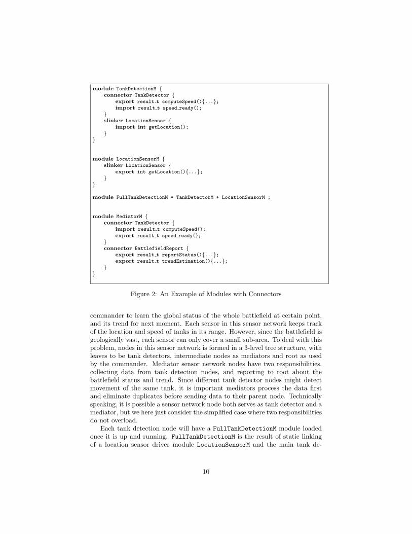
As explained earlier in Sec. 1, each module can define a list of communicationinterfaces called connectors, through which all communication behaviors of themodule happens. To illustrate how connectors work, we here give a simplifiedexample of battlefield sensoring in Fig. 2. Specific algorithm used for this sce-nario varies from application to application, and is independent of programminglanguage design. We here just provide one of the possible implementations todemonstrate our language features.
Here a battlefield teemed with tanks is scattered with hundreds of denselypopulated sensor network nodes for tank detection. The ultimate goal is for the
9
module TankDetectionM {connector TankDetector {
export result t computeSpeed(){...};import result t speed ready();
}slinker LocationSensor {
import int getLocation();
}}
module LocationSensorM {slinker LocationSensor {
export int getLocation(){...};}
}
module FullTankDetectionM = TankDetectorM + LocationSensorM ;
module MediatorM {connector TankDetector {
import result t computeSpeed();
export result t speed ready();
}connector BattlefieldReport {
export result t reportStatus(){...};export result t trendEstimation(){...};
}}
Figure 2: An Example of Modules with Connectors
commander to learn the global status of the whole battlefield at certain point,and its trend for next moment. Each sensor in this sensor network keeps trackof the location and speed of tanks in its range. However, since the battlefield isgeologically vast, each sensor can only cover a small sub-area. To deal with thisproblem, nodes in this sensor network is formed in a 3-level tree structure, withleaves to be tank detectors, intermediate nodes as mediators and root as usedby the commander. Mediator sensor network nodes have two responsibilities,collecting data from tank detection nodes, and reporting to root about thebattlefield status and trend. Since different tank detector nodes might detectmovement of the same tank, it is important mediators process the data firstand eliminate duplicates before sending data to their parent node. Technicallyspeaking, it is possible a sensor network node both serves as tank detector and amediator, but we here just consider the simplified case where two responsibilitiesdo not overload.
Each tank detection node will have a FullTankDetectionM module loadedonce it is up and running. FullTankDetectionM is the result of static linkingof a location sensor driver module LocationSensorM and the main tank de-
10

tection module TankDetectionM. Here TankDetectionM has a connector calledTankDetector, which according to our semantics for static linking, will alsobecome a connector for FullTankDetectionM. The connector has one exportfunction, computeSpeed, to compute the speed of the tank. Because of thesplit-phase nature of operations in connectors, a corresponding import functionspeed ready is provided, and at the end of the function body of computeSpeed,speed ready is supposed to be called.
Each mediator node will have a MediatorM module loaded once it is started.It has two connectors, TankDetector to communicate with tank detection nodes(collecting data), and BattlefieldReport to communicate with the root.
With this, MediatorM module can have a piece of code like the following,which might show up in any function defined in MediatorM:
// cref is a reference to module runtime created from FullTankDetectionM
x = connect cref at TankDetector;
x.computeSpeed();
x.disconnect;
It means the cell created from MediatorM initiates a connection with a cellcreated from a tank detection module FullTankDetectionM. The connector usedis TankDetector. The returned value of connect expression x is of connectiontype. With it, computeSpeed can be called. The connection can also be disabledafter mission is completed. This is the most basic use of connectors. Note crefcould be obtained in various ways, such as after an explicit dynamic loading(details in Sec. 2.5), or a value passed in as function parameters.
Stateful Connections The example in Fig. 2 gives an oversimplified examplewhere connectors are composed of a list of exported functions and a list ofimported functions. In reality, connections are almost always stateful (recallTCP for instance). Each connection always has something specific to itself toremember. For fulfilling this goal, our connector design also allows mutablefields as part of a connector definition.
In contrast with connection fields are cell fields. Our language also allowmodule runtimes to own application-specific states. The difference betweenconnector fields and cell fields is that each connection keeps a separate copy ofthe connector fields, but all connections to a single cell share the same cell state.For instance, if a cell has a connector TankDetector, all states that are specificto the connection, such as detection time length, should be kept as connectorfields. On the other hand, states that are deemed as the status of cell, such asthe location information of a sensor, should be kept as cell states.
Connector Generativity As a P2P operation, the established connectionvia connect expression is largely symmetric. However, since there is always aparty who initiates the connection and the other party who receives the request,the semantics of connect is also divided into two parts:
11

When a cell receives a request to connect to its certain connector, it gener-ates and initializes a new copy of connector fields. After that, all export functioncalls via this connector will be operating on this copy of connector states. Ourapproach is generative, which means new request to connect to the same con-nector will not supersede the previous one, or be denied due to the existing one;instead, new connections will be set up and multiple connections to the sameconnector can co-exist. Different connector requests to the same connector willnot interfere with each other: their connection states are separate, unless pro-grammer intentionally wants to; in that case cell states can be used for statesharing. Whenever a connection is established, a fresh session ID is generatedto tag the store for connection instances. The ID will be shared by the twoparties of the connection.
When a cell sends out a request for another cell to connect to its certainconnector, obviously the same generative approach is taken. Different from thereceiving party where all generative state handling is all hidden under the rug,programmers can actually get a handle to each connection, just as shown in thetank detection example. Here we brought to reader’s attention the rebindabilityof connectors:
// cref1, cref2 are pre-existing cell references
x = connect cref1 at TankDetector;
y = connect cref2 at TankDetector;
x.computeSpeed();
...
y.computeSpeed();
We therefore say, connections are generative in both directions.Connections are long-lived, in the sense that they are always there until
they are explicitly disconnected, via disconnect expression. In this case, allconnection states are removed from both sides for the specific connection. InSec. 2.6 we will see even if a cell migrates to a new physical location, its existingconnections will be carried over and kept alive.
Last we briefly discuss the static semantics of connector connection, thetyping issues. Basically the general rule is every import from one party has tobe satisfied by an export from the other party. However, it is allowed for eitherof the parties to have extra exports that are not matched. Connection fields arenot matched.
2.4 Location-Carefree Connections
The use of connectors in last section requires the connection initiator specifieswho it intends to communicate with, such as the cref1 and cref2 in last ex-ample. However, in many cases, the initiator does not really care what physicalnode it connects with, what it does care is the other party must satisfy itsneed for connection. The satisfaction process happens to fit well with connectorcompatibility checking. Therefore, any node that has a compatible connector
12

(with the same name, and all imported functions in the initiator’s connector areexports in the compatible node) will be connected. We call connection of thiskind location-carefree connection. The syntax for it is shown in the followingexample:
x = connect any at TankDetector;
x.computeSpeed();
Compared with regular Internet, sensor network is a very good fit for location-carefree connections. For one thing, the infrastructure of sensor network is wire-less, which implies for each sensor network node, it is very easy to broadcastthe request and wait for responses from any of the neighbor node. After all, allsensor network communication will be through broadcasting eventually. Sincesensor network is also typically dense, the latency for any neighbor to respondis usually low. For another reason, sensor network is typically formed by hun-dreds of nodes who are functionally the same, which means they have the sameconnectors. Normally when a request is sent, like retrieving a temperature orchecking the movement of a tank, it does not matter which sensor responds ina small locality. The bottom line is one of the nodes does respond.
2.5 Dynamic Module Loading/Unloading
Our programming language provides support for loading modules and unloadingtheir runtime form cells. This is important because running cells receive requestsand make responses, which would consume energy. Algorithms can be designedto detect in a given situation, what minimum set of sensor network nodes areneeded to keep the whole network correctly functioning. All the other nodes canjust be shut down or put to a sleeping state. When some nodes reach a powerdepletion, or the topology of the sensor network changes, the nodes can be againreactivated. This will involve dynamic loading and unloading of modules andcells.
Loading/Unloading Semantics A basic example to show the use of ourloading/unloading language construct is as follows:
// Module 0 is a pre-existing module name
x = load Module 0;
...
unload x;
The load process involves the creation of the cell runtime memory layout,including allocation of cell fields. The language construct assumes an implicitlookup process, which is given a module name, returning the code piece for themodule. For a sensor network node without permanent storage, this needs thesupport of virtual machine, where a code repository is associated.
The unloading process can unload cells from memory if its reference is given.The reference does not necessarily come from load. It can also be passed param-
13

eters or any sort already known to the program. A difficult issue is to considerthe handling of connection states. After all, a successful unloading will automat-ically disconnect all connections associated with the cell. We need a notificationmechanism in the semantics to explicitly disconnect all the connections beforeunloading.
2.6 Cell Migration
Sec. 1 justified the need to have migration supported as a core part of a program-ming language, so that different programmers can write out different migrationprocesses based on the need of their specific applications. A basic example toshow the use of our migration language construct is as follows:
// x is a pre-existing cell reference
migrate x to NodeID 1;
First we need to make clear the migration process needs to be atomic, i.e.it either succeeds without interruption, or it fails. In the following semanticsdescription, readers need to keep atomicity as an implicit requirement.
When the above expression is evaluated, cell referred to by x will inform allthe cells currently connecting to it, about the migration and the destination itintends to move to (in the example, NodeID 1). All the informed cells will henceupdate their states accordingly to record the change of the connections. Whenall are successfully done, the migrating cell serializes all its cell-level states andconnection states, unload itself from the memory of the current node, sends theserialized form to the new location, and at this new location loads the same codein, deserializes the state. The process also involves the backup and recovery ofexecution point.
All the internal states of the application, including the states of all its liv-ing connections, need to be preserved and transferred. The complexity andatomicity of this process justify why we treat migration as a first-class languageconstruct: a user-defined process would be error-prone, if possible at all.
From another perspective cell migration shows the long-livedness of connec-tions. Even when one of the connecting parties migrates to new physical nodes,original connections associated with the migrating cell are still kept alive. Con-nections are cut off only if they are explicitly disconnected or the cell is explicitlyunloaded from memory.
3 Formal Syntax
The abstract syntax of the language is shown in Fig. 3. Before elaboratingon details, we first reinstate the difference of two terms we use: module andcell. When we use the term module, we emphasize the code property of theprogram fragment, i.e., the static code piece that can be composed and loadedto memory; on the other hand, when we use the term cell, we emphasize theruntime property of the program, which can be taken as module after being
14

M ::= module µ {ε C S e} atomic module| module µ = µ1 + µ2 composed module| module µ = µ0 [n1 7→ n2] module with interface renaming
C ::= connector n {ε import ι export ι} connectorS ::= slinker n {import ι export ι} static linkerι ::= fn : τ {e} functionε ::= instn : τ state
e ::= x | cst variable, constant| cid | thiscell | thisconn cell reference| e.instn | e.instn :=e instance and its operations| n :: fn | e.fn | e(e) function and its operations| load µ | unload e load/unload| connect e at n | disconnect e connect/disconnect| connect any at n location-carefree connection| migrate e to ν migrate| e; e continuation
Tm ::= module {C S} module signature
Tc ::= cell {C} cell signatureτ ::= int | τ → τ | Tc | C type
ν node IDµ module namen interface namefn function nameinstn instance namecid cell ID
Figure 3: Abstract Syntax
loaded to memory and module runtime possessing states. Understanding thedifference between the two terms is important for understanding our language.
A module M can be formed in three ways. It is either an atomic module, ora composed module or a module with interface renaming. µ is the name of themodule:
• Atomic modules are formed with a list of static linkers (S), a list of connec-tors (C), a list of cell fields (ε), and initialization code for bootstrappingthe module when they are first loaded to memory (e). The overline de-notes a repetition of items; for instance X represents a list of Xs. Eachstatic linker has a name n, a list of functions to be imported (import ι),and a list of functions to be exported (export ι). We disallow the im-porting and exporting of states. Indeed, each state can be modeled bya get function and a set function, and whenever there is a need forstate to be exported/imported, a pair of get and set function can beexported/imported to achieve the same effect. Each connector also has aname n, a list of functions to be imported (import ι), and a list of func-tions to be exported (export ι). Different from static linkers, it can alsoown a list of connector fields (ε), which are used for stateful connections.
15

• Composed modules are simply formed by a “+” operator. µ1 + µ2 meansmodule with name µ1 and module with name µ2 are to be composedtogether.
• Modules with interface renaming have a syntax in the form of µ0 [n1 7→ n2].It means the resulting module is the same as module with name µ0, butinterface with name n1 is renamed to n2. If n2 is φ, it means interfacewith name n1 is removed. Here interface applies to both static linkers andconnectors.
Expressions (e) in the language include:
• variables (x) and constants (cst).
• cell reference constants, which include cell IDs (cid) or thiscell denotingthe cell reference to the current running cell itself.
• connection constants thisconn, denoting the current connection.
• state-related expressions. Depending on whether the state is a cell field ora connector field, these expressions are also in different forms. thiscell.instnis used to get the value of a cell field, e.n is used to get the value of aconnector field, where of course here e is a variable of connection type.e :=e is the expression to set state to new values.
• function-related expressions. n :: fn is used to refer to a function im-ported or exported in static linker with name n; e.fn is used to refer toa function associated with a connection where e has a connection type;When fn shows up, it should be understood as thisconn.fn. Finally, e(e)is standard function application.
• expressions for loading modules and unloading cells. load µ is used toload a module into memory where µ is the name of the module to beloaded. This expression returns a cell reference; unload e on the otherhand unloads a cell from memory, where e is of cell reference type. Here ecan either be a CID constant, or thiscell, a reference obtained from load,or a reference passed in as a function parameter.
• expressions for connecting and disconnecting cells. connect e at n is usedto connect to cell(s) referred to by cell reference e; the connector to beconnected is of name n. The expression returns a variable of connectiontype. disconnect e disconnects the connection represented by e (e here isof connection type). connect any at n is used to initiate location-carefreeconnections.
• expression for migrating cells. migrate e to ν is used to migrate cellreferred to by cell reference e to a new node identified by ν.
• e1; e2 is sequencing of expressions. It means evaluating e1 first, and thene2.
16

Types of the language include a module signature and a cell signature. As wecan see, module signature includes the connectors and static linkers of the mod-ule, and yet cell signature only includes the runtime interfaces of the module,which are connectors. Besides, we also support basic types like integers (int),function types (τ → τ) and connection type, which is the same as declarationof a connector.
4 Cell Runtime Design
Starting from this section, this report demonstrates how a language we justdefined can be mapped to an implementation. As discussed in Sec. 2.1, theapproach we take is intermediate: we will show a possible design that is low-level enough to be directly implemented, and yet does not limit itself to just onespecific implementation to a specific operating system. In this section, we firstgive a description of cell runtime representation. In Section 5 and 6, we givea specification of our virtual machine. In Section 7, a description of languagesemantics is given.
At post-compilation time, modules can take different forms depending onimplementation. They could be in regular binary code form, or in bytecodeform similar to Java bytecode, or intermediate code capsules created by Mate.A close analogy of post-compilation modules in our design would be class filesin Java. Since typical sensors do not have permanent storage associated withthem, we here assume post-compilation modules are also kept in memory, withtype ModuleType. Note this kind of memory habitants are different from cells;the latter would be analogously thought of as objects in Java.
Cell Runtime Memory Layout When a module is loaded, a cell is createdusing the module as code template. In this section, the focus of our attention ison the runtime memory layout of cells; the loading process itself will be detailedlater in Sec. 6.5.
The runtime memory representation of a cell can be demonstrated by thefollowing type:
# define MAX CELL FIELD 100# define MAX CONN 100type CellType = struct {
ConnType ct [MAX CONN];State ft [MAX CELL FIELD];string µ;
};It indicates each cell runtime is composed of: 1) ct, a list of states recordingthe status of live connections the cell currently keeps. We sometimes call itconnection table of a cell; 2) ft, a list of states recording the values of cell fields;3) µ, the name of the codebase module of the cell. Type State and ConnTypeare defined below:
17

# define MAX CONN FIELD 100type State = struct {
string label ;VAL value;
};type ConnType = struct {
ConnID connid ;string connName;CID connectTo;State st [MAX CONN FIELD];
};According to the definition above, a connection is recorded with its connectionID (connid), the name of the connector involved in the connection (connName),the CID of the party being connected (connectTo), and a list of per-connectionstates (st).
Some Housekeeping Operations Several local housekeeping operations aredefined on data structures introduced above. These operations are mostly get-ters and setters of related data structures; we simply list them here, instead ofgiving full definitions. They will be used in later sections when we define morecomplicated operations:
• updateConnT(cid, connid, connName, connectTo, st) updates cell cid’s con-nection table, in which the entry representing connection with ID connidis modified with the new tuple 〈connid, connName, connectTo, st〉.
• newConnT(cid, connid, connName, connectTo) adds to cell cid’s connec-tion table one new entry, 〈connid, connName, connectTo, st〉, where st isthe initial per-connection state of connector connName of cell cid.
• lookupConnT(cid, connid) returns the entry indexed by connid of cell cid’sconnection table.
• removeConnT(cid, connid) removes the entry indexed by connid from cellcid’s connection table.
• updateCellSt(cid, label, value) updates cell cid’s field, where the valuelabeled by label is changed to value.
• lookupCellSt(cid, label) returns the value of cell field indexed by label ofcell cid.
• initCellSt(mh) returns the initial cell-level state after module referencedby mh is loaded.
• updatePerConnSt(cid, connid, label, value) updates cell cid’s field in con-nection connid, and the label of the field is label. After updating, thefield is set to value.
18

• lookupPerConnSt(cid, connid, label) returns the value of cid’s field in con-nection connid, and the label of the field is label.
5 Virtual Machine Design: Data Structures
Each sensor has a virtual machine running on top of it. Multiple cells can runon the same virtual machine. Each virtual machine owns some global data,and provides several built-in services that will be used by programs written inour language. In this section, we specify virtual machine level data structures.Virtual machine built-in services will be specified in Sec. 6.
5.1 Standard Data Structures
Same as traditional models, our virtual machine also holds the following stan-dard data structures:
• a call stack, with each frame owning a local variable area and an operandstack. The difference for our language is, whenever a function call is fired,two parameters will be put onto operand stack automatically, the cell IDthe function belongs to, and the connection ID the function invocation iscurrently engaged in. Details on this subject will be discussed in Sec. 6.1.
• a program counter, the execution pointer indicative of where the currentexecution runs for the cell. Since in our virtual machine design, all cellsshare one thread, the program counter will need to consist of two parts:the CID of the cell currently in execution, and the pointer to point to thenext instruction in the code area of the cell.
5.2 Module Location Table
Each virtual machine holds a table, module location table (shorthanded as MLT),which keeps record of the modules sitting on a particular sensor network node.It adopts the following form, defined as mlt:
# define MAX MLT 100type ModuleLocRecord = struct {
string µ;ModuleType ∗ mh;
};ModuleLocRecord mlt[MAX MLT];
Notation (*) is used here (and several definitions in later sections) to de-note reference to a data structure. Readers should not confuse this level ofrepresentation with our source language.
Two local operations are defined on MLT, which will be used in later sections:
19

• updateMLT(µ,mh) updates the virtual machine’s MLT, in which the entryrepresenting module with name name is modified with new new locationpointer mh. If the entry for name does not exist, the operation append anew entry to the table.
• lookupMLT(µ) returns the entry indexed by µ of the virtual machine’sMLT.
5.3 Cell Location Table
Each virtual machine holds a table, cell location table (shorthanded as CLT),which keeps record of the location information of cells. It adopts the followingform, defined as clt:
# define MAX CLT 100type Status = enum {Active, Remote};type LocType = union {
CellType ∗ ch;NetAddr ν;
};type CellLocRecord = struct {
CID cid;Status sts;LocType loc;
};CellLocRecord clt[MAX CLT];
Each entry of CLT (with type CellLocRecord) indicates the location to findthe cell with ID cid. There is a status flag (sts) in the data structure, whichcan represent two different cases, and the type of loc depends on the value ofthe status flag:
• The cell is currently running on the same virtual machine. In this case,the loc field will keep record of the cell handle, which has type CellType*.The flag is set to Active.
• The cell is currently on a different sensor node. In this case, the loc fieldwill keep record of the sensor node information. NetAddr is a built-in type.Depending on implementation, it could be the MAC address associatedwith sensor networks, or any identifier which can uniquely find a specificvirtual machine on a remote site.
The reason why CLT not just has entries about cells running on top of theCLT-owning virtual machine, but also has entries about cells on other virtualmachines is realistically each sensor node is supposed to know its neighbor infor-mation. Sensor network at low level is broadcast network in nature. It is theseneighbor sensors a particular sensor is able to communicate with. It is thereforeimportant for a virtual machine, at any give time, to keep an active record of
20
what are the neighbors of its lodging sensor. The maintenance of neighbor tableis a task for the virtual machine. Its protocol varies depending on many factorssuch as efficiency and energy preservation requirements. It is initialized whensensor networks are laid out, and can be refreshed periodically. This helps forlocation-carefree operation.
In addition, since we allow cell migration, it is possible that requests are sentto a sensor after the cell has moved to another sensor. We need a forwardingmechanism.
Several local operations are defined on CLT, which will be used in latersections:
• updateCLT(cid, sts, loc) updates the virtual machine’s CLT, in which theentry representing cell cid is modified with new status sts and new locationloc. If the entry for cell cid does not exist, the operation append a newentry to the table.
• lookupCLT(cid) returns the entry indexed by cid of the virtual machine’sCLT.
• randomSelectNeighbor(n) randomly selects a cid from the list of cell IDsappearing in the virtual machine’s neighbor table. The selected one musthave a connector n.
6 Virtual Machine Design: Built-in Services
Here we specify the built-in services each virtual machine is expected to have.A program written in our language will depend on the correct running of thevirtual machines. Some of our language constructs will be compiled to a formusing these primitives; built-in services of virtual machines therefore also forman indispensable part of our language core. A summary of the built-in servicesis as follows:
6.1 call: Function Invocation Service
Function invocation is a basic service available to essentially every virtual ma-chine design. In our virtual machine, the service has the following interface:
call(CID cid, ConnID connid, string fn, string ifn, VAL v);
which denotes invoking a function named fn with parameter v, defined in cellcid. There are two cases: 1) if the function is defined in a connector, connidis the ID of the current connection. In this case, ifn is set to NULL STR; 2) ifthe function is defined in a static linker, ifn is the name of the static linker. Inthis case, connid is set to NULL CONNID. Here the difference originates from thefact that if the function is in a static linker, static linker name and functionname combined is enough for all information to invoke the function; however ifthe function is in a connector, connector name and function name combined is
21

not enough, since the function needs to know what the current connection is, todecide on which copy of the connection fields it operates on.
The service first locate the code entry for function fn. This is not a difficulttask because cell runtime representation already has its codebase information(See Sec. 4). The point that deserves attention is that when the function callhappens, not just v is pushed to operand stack; two more values are also putto stack: cid, the CID of the current cell, and connid, the connection ID of thecurrent connection. Thus, inside the function, code can refer to these two valuesusing thiscell and thisconn. This handling is very similar to that of the thispointer of object-oriented languages like C++ and Java.
6.2 Serialization/Deserialization Services
Serialization is the crucial process to preserve cell states when cells migratefrom one sensor to another; we expect the states of cells are kept and restoredwhen they arrive at the new virtual machine. Deserialization is the dual ofserialization, which deals with restoration of serialized data. The two serviceshave the following signatures:
SerializedForm serialize(CID ∗ cid);
CID deserialize(SerializedForm sf);
A serialized form of cells has type SerializedForm, which is defined as follows:
type SerializedState = struct {string label ;SerializedVAL value;
};type SerializedConnType = struct {
ConnID connid ;string conname;CID connectTo;SerializedState sst [MAX CONN STATE];
};type SerializedForm = struct {
CID cid;ModuleType m;SerializedConnType sct [MAX CONN];SerializedState sft [MAX CELL STATE];
};
The definition indicates a serialized cell is composed of: 1) cell ID; 2) codebaseof the serialized cell, of type ModuleType; 3) serialized connection fields record-ing live connection information, of type SerializedConnType; 4) serialized cellfields of type SerializedState.
Serialization and deserialization of data types (type SerializedVAL) are nottrivial issues. Although the current definition of our language does not support
22

many data types like pointers and objects since the pick of these data types arealmost orthogonal to the issues we are interested, but in a realistic language,references and objects should always be supported. In a C like language, if apointer is serialized, the data that is pointed to are also expected to be serial-ized. In a Java like language, if an object is serialized, any field of the objectalso needs to be serialized. Since a pointer might contain another pointer inside,or an object has another object as a field, the serialization process will operatehierarchically on the data to be serialized. When recursion happens, the pro-cess also needs to make sure cycles are taken care of to avoid non-termination.The process is largely standard; interested readers can refer to [LY99] for adescription of Java’s serialization process.
Deserialization inevitably involves a process of constructing cell runtimememory layout. It differs from load in the sense that load only initialize cellfields and connection fields, and yet deserialize recovers states from serializeddata. At the end of the deserialization process, updateCLT(cid, Active, ch) isinvoked, where cid is the ID of the just deserialized cell (this information isinside serialized form), and ch is the pointer to the cell runtime memory area.This virtual machine thus acknowledges the existence of cell cid, active on topof it.
6.3 send: Virtual Machine Message Sending Service
Built-in service send sends a request to a cell potentially located on a differentvirtual machine and sensor. It signature is as follows:
send(NetAddrν, CID source, CID dest, Request req);
which denotes a request req is sent to location ν. The receiving cell has a CIDdest, locating on top of a virtual machine at location ν. The request is sent bycell source. Because of migration, a request might need to be forwarded if a cellhas already moved to another virtual machine. It is therefore not always truethat source is the party invoking send.
6.4 receive: Virtual Machine Message Listening Service
Built-in service receive is a message handler of the virtual machine. It isautomatically triggered when requests sent via send are received. From a low-level view, any inter-cell communications are mediated by virtual machines,which implies, any invocations sent to a specific cell will first be received bythe virtual machine of the cell, and then the message listener receive of thevirtual machine will decide on how to handle it. The service has the followingsignature:
receive(CID source, CID dest, Request req);
which denotes a request req is received by the current virtual machine, and itis sent from cell source, and it is sent to cell dest sitting on the current virtual
23

machine. Either source or dest can also be set to be VM, which denotes therequest is sent from the current virtual machine, or sent to the current virtualmachine, instead of a specific cell sitting on top of it.
We omit the formal definition of Request type here, but it is indeed astraightforward union type of various record types, each of which representsa request format. Each record type has its first field set to the flag representingthe kind of request, followed by a list of parameters needed by the specific kindof request. Request flags can be to Deserialize, NewConn, DisConn, CallConnand UpdateLoc, as we will see shortly. We define receive mathematically usingcase analysis on request format, as follows:
receive(s, VM, 〈Deserialize, sf〉) def= deserialize(sf);receive(s, d, 〈NewConn, connid, n〉) def= newConnT(d, connid, n, s);
if〈d, Active, ch〉 = lookupCLT(d)receive(s, d, 〈NewConn, connid, n〉) def= send(ν, s, d, 〈NewConn, connid, n〉);
if〈d, Remote, ν〉 = lookupCLT(d)receive(s, d, 〈DisConn, connid〉) def= removeConnT(d, connid);
receive(s, d, 〈CallConn, connid, fn, v〉) def= call(d, connid, fn, NONE, v);
receive(s, VM, 〈UpdateLoc, ν〉) def= updateCLT(s, Remote, ν);
The request handler definition is largely self-explaining. In the first case,when a deserialization request is received, the virtual machine deserializes theserialized data sf. In the second and third cases, a request to set up a newconnection with cell d is fired. If d is located on the receiving virtual machine,connection table is updated (the second case); if d is located on a remote vir-tual machine, the current virtual machine simply forwards the request. This ispossible because of cell migration. In the third case, a request for disconnectionmeans the removal of a connection table entry. In the fourth case, a requestto invoke a function in a connector mostly hinges on the invocation of systemservice, the call service. In the fifth case, a request to update location infor-mation of a cell, which is useful for cell migration, indicates an update on theneighbor table of the virtual machine.
6.5 Loading/Unloading Services
Service load provides the functionality of preparing a cell runtime memorylayout from its codebase module; in contrast, service unload provides the func-tionality of releasing the memory area a cell occupies, such as its cell states,connection states, local variable pool and call stack. Loading and unloadingservices are important for sensor programming; with them, modules can beflexibly loaded into memory when they are needed, and memory can be freedwhen the functionalities provided by the cell are not useful any more. The
24

signature for these services are:
CID load(string µ);
string unload(CID cid);
First, service load can be defined as follows:
#define NULL CONNT nullload(µ) def= cid = newCID();
ch = alloc(NULL CONNT, initCellSt(µ), µ〉);updateCLT(cid, Active, ch);cid
In this definition, cid is the ID of the newly created cell, whose codebase isset to the module with name µ. The cell’s initial connection table is empty(NULL CONNT) and its initial cell fields are initialized. load service then updatesCLT to reflect the addition of cell cid to the virtual machine. Finally, loadservie returns the cell ID of the newly created cell.
Correspondingly, unload service is defined as below. All cells keeping anactive connection with the soon-to-be-unloaded cell will be sent a disconnectionmessage, and the memory area allocated for the cell is freed:
unload(cid) def= 〈cid, Active, ch〉 = lookupCLT(cid);〈ct, ft, µ〉 = ∗ch;
foreach 〈connid, n, cid′, st〉 in ct〈cid′, Remote, ν′〉 = lookupCLT(cid′);req = 〈DisConn, connid〉;send(ν′, cid, cid′, req);
free(ch);µ;
Note that since we take the simple threading model for our virtual machinedesign, loading process does not create new thread. Consequently, we do notallow cells to execute at the same time. The initialization code of the loadedcell is not executed. They can be accessed by the loading cell via expressionslike connect, etc. We have achieved multiple cells running on the same virtualmachine without using multithreading.
7 Semi-formal Language Semantics
In this section, we present the semantics of our language. Instead of takingthe usual formal approach, we intentionally define each language expression asa semi-formal program. This is because, mathematical formalizations can hidesome details that still make a difference during implementation. As a systemproject in nature, we believe a semi-formal specification is more appropriate, asit is more precise specification of implementation.
25

Here we define the meaning function J . K, whose domain is the set of expres-sions belonging to our language, and whose range is the set of programs whosecontrol flow can be directly mapped to low-level virtual machine operations.J e K denotes the meaning of expression e. Readers are advised that these def-initions should not be read as macros. For each expression defined below, thecorrectness of semantics is hinged on atomicity of the expression.
7.1 Cell Bootstrapping
For any realistic language, there is always this first question to ask: how couldthe first runtime be established? We here define it below. Notice that it isnot part of source language expressions; instead, readers should set analogybetween this and typing in java HelloWorld in the command line of Javavirtual machine:
J bootstrap µ K def= cid = load(µ);init(cid);
Here µ is the name of the module to be loaded. The virtual machine first loadthe cell based on its code base module with name µ, followed by init(cid), asimple function to execute the initialization code of the cell, which is definedas part of module syntax (recall Sec. 3 for the grammar). This is the pointexecution of code starts.
According to the syntax of our language, we have two other ways to definemodules: composed modules and modules with renamed interfaces. Bootstrap-ping these two kinds of modules is exactly the same as what we just describedabove. In fact, these two are only concerned with transformations of code, anddoes not have runtime effect. At compile time, the composed modules will bemerged; modules with renamed interfaces will have them renamed. When itbears the ModuleType in our system, the code will look exactly like an atomicmodule. We leave out the part of code transformations of the two cases, sincethey are fairly intuitive.
7.2 Cell Dynamic Loading/Unloading
We next define the semantics of dynamic loading and unloading. Dynamicloading process is almost the same as bootstrapping process, except that theloaded cell does not run its initialization code. Dynamic unloading directly callson unload service.
J load µ K def= load(µ)J unload e K def= unload(J e K)
7.3 Cell Connection Establishment
Cell connection establishment involves two parties, the initiating party and ini-tiated party. For the initiating party, all needs to be done is to add one more
26

entry to the cell’s connection table, recording the newly established connection.For the initiated party, there are two cases: 1) if the initiated party sits on aremote node, a request needs to be sent, which is the NewConn request as wedemonstrate below; 2) if the initiated party sits on the same node, a directchange of connection table is issued. Whenever a new connection is established,a new connection ID is set up via newConnID function.
J connect e at n K def= cid = J e K;connid = newConnID();case lookupCLT(cid) of〈cid, Remote, ν〉 :
req = 〈NewConn, connid, n〉;send(ν, thiscell, cid, req);
〈cid, Active, ch〉 :newConnT(cid, connid, n, thiscell);
newConnT(thiscell, connid, n, cid);connid;
For location-carefree connections, it is basically a random selection of neighborcells first, and then connect to the cell:
J connect any at n K def= cid = randomSelectNeighbor(n);J connect cid at n K
7.4 Cell Disconnection
Just as cell connection establishment, cell disconnection also involves two par-ties, the initiating party and initiated party. For the initiating party, all needs tobe done is to remove the entry from the cell’s connection table, the one record-ing the connection. For the initiated party, similarly two cases are possible:
J disconnect e K def= connid = J e K;〈connid, n, cid, st〉 = lookupConnT(thiscell, connid);case lookupCLT(cid) of〈cid, Remote, ν〉 :
req = 〈DisConn, connid〉;send(ν, thiscell, cid, req);
〈cid, Active, ch〉 :removeConnT(cid, connid);
removeConnT(thiscell, connid);
7.5 Cell Field Access
The following two define the semantics for cell field access related expressions:
J thiscell.instn K def= lookupCellSt(thiscell, instn);J thiscell.instn := e K def= updateCellSt(thiscell, instn, J e K);
27
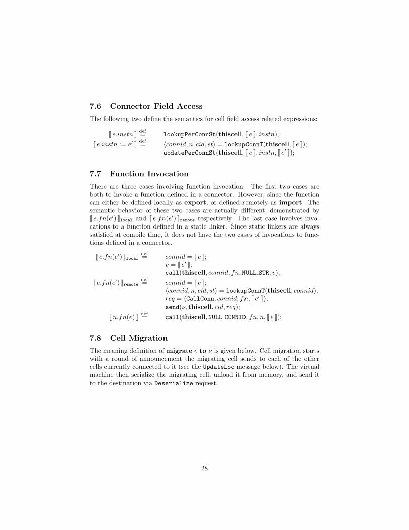
7.6 Connector Field Access
The following two define the semantics for cell field access related expressions:
J e.instn K def= lookupPerConnSt(thiscell, J e K, instn);J e.instn := e′ K def= 〈connid, n, cid, st〉 = lookupConnT(thiscell, J e K);
updatePerConnSt(thiscell, J e K, instn, J e′ K);
7.7 Function Invocation
There are three cases involving function invocation. The first two cases areboth to invoke a function defined in a connector. However, since the functioncan either be defined locally as export, or defined remotely as import. Thesemantic behavior of these two cases are actually different, demonstrated byJ e.fn(e′) Klocal and J e.fn(e′) Kremote respectively. The last case involves invo-cations to a function defined in a static linker. Since static linkers are alwayssatisfied at compile time, it does not have the two cases of invocations to func-tions defined in a connector.
J e.fn(e′) Klocaldef= connid = J e K;
v = J e′ K;call(thiscell, connid, fn, NULL STR, v);
J e.fn(e′) Kremotedef= connid = J e K;
〈connid, n, cid, st〉 = lookupConnT(thiscell, connid);req = 〈CallConn, connid, fn, J e′ K〉;send(ν, thiscell, cid, req);
Jn.fn(e) K def= call(thiscell, NULL CONNID, fn, n, J e K);
7.8 Cell Migration
The meaning definition of migrate e to ν is given below. Cell migration startswith a round of announcement the migrating cell sends to each of the othercells currently connected to it (see the UpdateLoc message below). The virtualmachine then serialize the migrating cell, unload it from memory, and send itto the destination via Deserialize request.
28
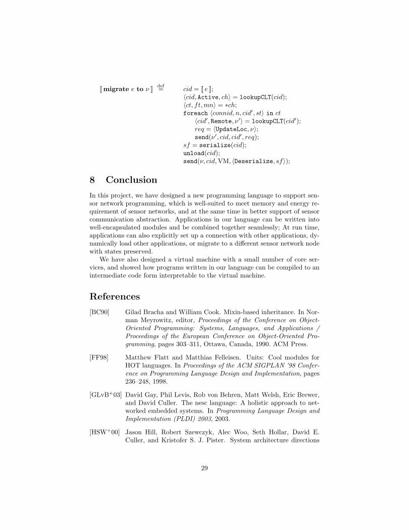
J migrate e to ν K def= cid = J e K;〈cid, Active, ch〉 = lookupCLT(cid);〈ct, ft,mn〉 = ∗ch;foreach 〈connid, n, cid′, st〉 in ct〈cid′, Remote, ν′〉 = lookupCLT(cid′);req = 〈UpdateLoc, ν〉;send(ν′, cid, cid′, req);
sf = serialize(cid);unload(cid);send(ν, cid,VM, 〈Deserialize, sf〉);
8 Conclusion
In this project, we have designed a new programming language to support sen-sor network programming, which is well-suited to meet memory and energy re-quirement of sensor networks, and at the same time in better support of sensorcommunication abstraction. Applications in our language can be written intowell-encapsulated modules and be combined together seamlessly; At run time,applications can also explicitly set up a connection with other applications, dy-namically load other applications, or migrate to a different sensor network nodewith states preserved.
We have also designed a virtual machine with a small number of core ser-vices, and showed how programs written in our language can be compiled to anintermediate code form interpretable to the virtual machine.
References
[BC90] Gilad Bracha and William Cook. Mixin-based inheritance. In Nor-man Meyrowitz, editor, Proceedings of the Conference on Object-Oriented Programming: Systems, Languages, and Applications /Proceedings of the European Conference on Object-Oriented Pro-gramming, pages 303–311, Ottawa, Canada, 1990. ACM Press.
[FF98] Matthew Flatt and Matthias Felleisen. Units: Cool modules forHOT languages. In Proceedings of the ACM SIGPLAN ’98 Confer-ence on Programming Language Design and Implementation, pages236–248, 1998.
[GLvB+03] David Gay, Phil Levis, Rob von Behren, Matt Welsh, Eric Brewer,and David Culler. The nesc language: A holistic approach to net-worked embedded systems. In Programming Language Design andImplementation (PLDI) 2003, 2003.
[HSW+00] Jason Hill, Robert Szewczyk, Alec Woo, Seth Hollar, David E.Culler, and Kristofer S. J. Pister. System architecture directions
29
for networked sensors. In Architectural Support for ProgrammingLanguages and Operating Systems, pages 93–104, 2000.
[JS00] Jerry James and Ambuj Singh. Design of the Kan distributed ob-ject system. Concurrency: Practice and Experience, 12(8):755–797,2000.
[LC02] P. Levis and D. Culler. Mate: A tiny virtual machine for sensornetworks. In International Conference on Architectural Support forProgramming Languages and Operating Systems, San Jose, CA,USA, Oct. 2002. To appear.
[LY99] T. Lindholm and F. Yellin. The Java Virtual Machine Specification(Second Edition). Addison-Wesley, 1999.
[MFH02] Samuel Madden, Michael J. Franklin, and Joseph M. Hellerstein.Tag: a tiny aggregation service for ad-hoc sensor networks. In 5thAnnual Symposium on Operating Systems Design and Implemena-tion(OSDI), Dec. 2002.
[RFS+00] Alastair Reid, Matthew Flatt, Leigh Stoller, Jay Lepreau, and EricEide. Knit: Component composition for systems software. In Proc.of the 4th Operating Systems Design and Implementation (OSDI),pages 347–360, 2000.
30