professional opinion no. 2009/02 a probabilistic tsunami
TRANSCRIPT
COMMERICAL-IN-CONFIDENCE
Professional Opinion No. 2009/02
A Probabilistic Tsunami HazardAssessment of the
Southwest Pacific Nations
Christopher Thomas and David Burbidge
Risk and Impact Analysis Group
Geoscience Australia
February 4, 2009
PREPARED FOR:Australian Government - AusAID
South Pacific Applied Geoscience Commission(SOPAC)

Department of Resources, Energy and TourismMinister for Resources, Energy and Tourism: The Hon. Martin Ferguson, MPSecretary: Dr Peter Boxall
Geoscience AustraliaChief Executive Officer: Dr Neil Williams
c©Commonwealth of Australia 2009
This work is for internal government use only and no part of this product may be repro-duced, distributed or displayed publicly by any process without the permission of the ChiefExecutive Officer, Geoscience Australia. Requests and enquiries should be directed to theChief Executive Officer, Geoscience Australia, GPO Box 378 Canberra ACT 2601.
Geoscience Australia has tried to make the information in the product as accurate aspossible. However, it does not guarantee that the information is totally accurate or com-plete. Therefore, you should not solely rely on this information when making a commercialdecision.
GeoCat No. 68193
Bibliographic reference: Thomas, C. and Burbidge, D. 2009. A Probabilistic TsunamiHazard Assessment of the Southwest Pacific Nations. Geoscience Australia ProfessionalOpinion. No.2009/02
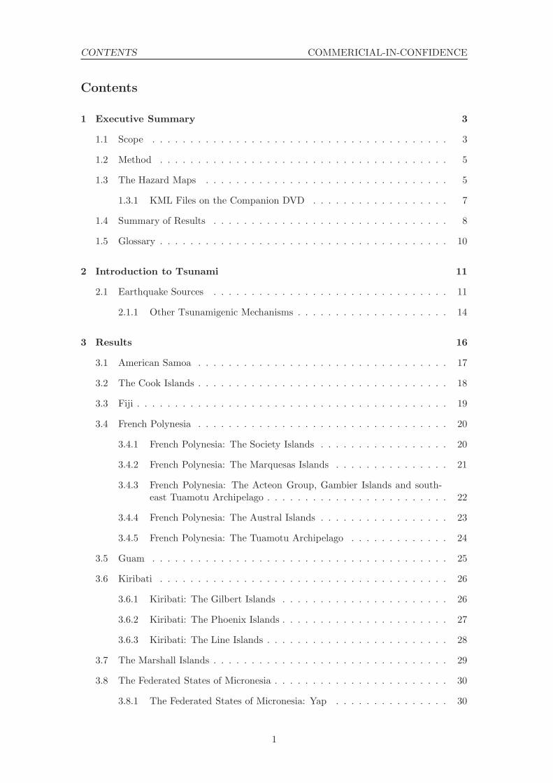
CONTENTS COMMERICIAL-IN-CONFIDENCE
Contents
1 Executive Summary 3
1.1 Scope . . . . . . . . . . . . . . . . . . . . . . . . . . . . . . . . . . . . . . . 3
1.2 Method . . . . . . . . . . . . . . . . . . . . . . . . . . . . . . . . . . . . . . 5
1.3 The Hazard Maps . . . . . . . . . . . . . . . . . . . . . . . . . . . . . . . . 5
1.3.1 KML Files on the Companion DVD . . . . . . . . . . . . . . . . . . 7
1.4 Summary of Results . . . . . . . . . . . . . . . . . . . . . . . . . . . . . . . 8
1.5 Glossary . . . . . . . . . . . . . . . . . . . . . . . . . . . . . . . . . . . . . . 10
2 Introduction to Tsunami 11
2.1 Earthquake Sources . . . . . . . . . . . . . . . . . . . . . . . . . . . . . . . 11
2.1.1 Other Tsunamigenic Mechanisms . . . . . . . . . . . . . . . . . . . . 14
3 Results 16
3.1 American Samoa . . . . . . . . . . . . . . . . . . . . . . . . . . . . . . . . . 17
3.2 The Cook Islands . . . . . . . . . . . . . . . . . . . . . . . . . . . . . . . . . 18
3.3 Fiji . . . . . . . . . . . . . . . . . . . . . . . . . . . . . . . . . . . . . . . . . 19
3.4 French Polynesia . . . . . . . . . . . . . . . . . . . . . . . . . . . . . . . . . 20
3.4.1 French Polynesia: The Society Islands . . . . . . . . . . . . . . . . . 20
3.4.2 French Polynesia: The Marquesas Islands . . . . . . . . . . . . . . . 21
3.4.3 French Polynesia: The Acteon Group, Gambier Islands and south-east Tuamotu Archipelago . . . . . . . . . . . . . . . . . . . . . . . . 22
3.4.4 French Polynesia: The Austral Islands . . . . . . . . . . . . . . . . . 23
3.4.5 French Polynesia: The Tuamotu Archipelago . . . . . . . . . . . . . 24
3.5 Guam . . . . . . . . . . . . . . . . . . . . . . . . . . . . . . . . . . . . . . . 25
3.6 Kiribati . . . . . . . . . . . . . . . . . . . . . . . . . . . . . . . . . . . . . . 26
3.6.1 Kiribati: The Gilbert Islands . . . . . . . . . . . . . . . . . . . . . . 26
3.6.2 Kiribati: The Phoenix Islands . . . . . . . . . . . . . . . . . . . . . . 27
3.6.3 Kiribati: The Line Islands . . . . . . . . . . . . . . . . . . . . . . . . 28
3.7 The Marshall Islands . . . . . . . . . . . . . . . . . . . . . . . . . . . . . . . 29
3.8 The Federated States of Micronesia . . . . . . . . . . . . . . . . . . . . . . . 30
3.8.1 The Federated States of Micronesia: Yap . . . . . . . . . . . . . . . 30
1

CONTENTS COMMERICIAL-IN-CONFIDENCE
3.8.2 The Federated States of Micronesia: Chuuk . . . . . . . . . . . . . . 31
3.8.3 Federated States of Micronesia: Pohnpei and Kosrae . . . . . . . . . 32
3.9 Nauru . . . . . . . . . . . . . . . . . . . . . . . . . . . . . . . . . . . . . . . 33
3.10 New Caledonia . . . . . . . . . . . . . . . . . . . . . . . . . . . . . . . . . . 34
3.11 Niue . . . . . . . . . . . . . . . . . . . . . . . . . . . . . . . . . . . . . . . . 35
3.12 Palau . . . . . . . . . . . . . . . . . . . . . . . . . . . . . . . . . . . . . . . 36
3.13 Papua New Guinea . . . . . . . . . . . . . . . . . . . . . . . . . . . . . . . . 37
3.13.1 Papua New Guinea: New Britain, New Ireland and Bougainville . . 37
3.13.2 Papua New Guinea: South and West . . . . . . . . . . . . . . . . . . 38
3.14 Samoa . . . . . . . . . . . . . . . . . . . . . . . . . . . . . . . . . . . . . . . 39
3.15 The Solomon Islands . . . . . . . . . . . . . . . . . . . . . . . . . . . . . . . 40
3.16 Tokelau . . . . . . . . . . . . . . . . . . . . . . . . . . . . . . . . . . . . . . 41
3.17 Tonga . . . . . . . . . . . . . . . . . . . . . . . . . . . . . . . . . . . . . . . 42
3.18 Tuvalu . . . . . . . . . . . . . . . . . . . . . . . . . . . . . . . . . . . . . . . 43
3.19 Vanuatu . . . . . . . . . . . . . . . . . . . . . . . . . . . . . . . . . . . . . . 44
4 Conclusion 45
A PTHA Method 49
A.1 Summary . . . . . . . . . . . . . . . . . . . . . . . . . . . . . . . . . . . . . 49
A.2 Bathymetry . . . . . . . . . . . . . . . . . . . . . . . . . . . . . . . . . . . . 49
A.3 Model Output Points . . . . . . . . . . . . . . . . . . . . . . . . . . . . . . . 51
A.4 Fault Model . . . . . . . . . . . . . . . . . . . . . . . . . . . . . . . . . . . . 51
A.5 Numerical Modelling of Sea Floor Deformation and Tsunami Propagation . 51
A.6 Catalogue of Synthetic Earthquakes . . . . . . . . . . . . . . . . . . . . . . 51
A.7 Deaggregating the Hazard . . . . . . . . . . . . . . . . . . . . . . . . . . . . 52
A.7.1 Deaggregated Hazard Maps . . . . . . . . . . . . . . . . . . . . . . . 52
A.8 Regional Weighted Deaggregated Hazard Maps . . . . . . . . . . . . . . . . 53
B Validation: Kuril Islands, 15/11/2006 54
C Validation: Chile, 22/05/1960 58
2
1 EXECUTIVE SUMMARY COMMERICIAL-IN-CONFIDENCE
1 Executive Summary
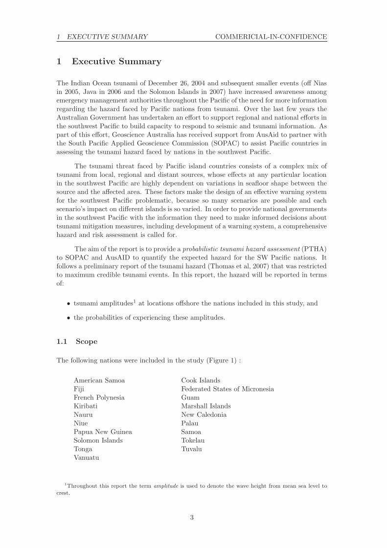
The Indian Ocean tsunami of December 26, 2004 and subsequent smaller events (off Niasin 2005, Java in 2006 and the Solomon Islands in 2007) have increased awareness amongemergency management authorities throughout the Pacific of the need for more informationregarding the hazard faced by Pacific nations from tsunami. Over the last few years theAustralian Government has undertaken an effort to support regional and national efforts inthe southwest Pacific to build capacity to respond to seismic and tsunami information. Aspart of this effort, Geoscience Australia has received support from AusAid to partner withthe South Pacific Applied Geoscience Commission (SOPAC) to assist Pacific countries inassessing the tsunami hazard faced by nations in the southwest Pacific.
The tsunami threat faced by Pacific island countries consists of a complex mix oftsunami from local, regional and distant sources, whose effects at any particular locationin the southwest Pacific are highly dependent on variations in seafloor shape between thesource and the affected area. These factors make the design of an effective warning systemfor the southwest Pacific problematic, because so many scenarios are possible and eachscenario’s impact on different islands is so varied. In order to provide national governmentsin the southwest Pacific with the information they need to make informed decisions abouttsunami mitigation measures, including development of a warning system, a comprehensivehazard and risk assessment is called for.
The aim of the report is to provide a probabilistic tsunami hazard assessment (PTHA)to SOPAC and AusAID to quantify the expected hazard for the SW Pacific nations. Itfollows a preliminary report of the tsunami hazard (Thomas et al, 2007) that was restrictedto maximum credible tsunami events. In this report, the hazard will be reported in termsof:
• tsunami amplitudes1 at locations offshore the nations included in this study, and
• the probabilities of experiencing these amplitudes.
1.1 Scope
The following nations were included in the study (Figure 1) :
American Samoa Cook IslandsFiji Federated States of MicronesiaFrench Polynesia GuamKiribati Marshall IslandsNauru New CaledoniaNiue PalauPapua New Guinea SamoaSolomon Islands TokelauTonga TuvaluVanuatu
1Throughout this report the term amplitude is used to denote the wave height from mean sea level tocrest.
3

1 EXECUTIVE SUMMARY COMMERICIAL-IN-CONFIDENCE
140˚ 160˚ 180˚ 200˚ 220˚ 240˚
−20˚
0˚
20˚
American Samoa
Cook
Isla
nds
French PolynesiaFiji
Guam
Kiribati
Marshall IslandsMicronesia
New CaledoniaNiue
Palau
Papua New Guinea
Solomon Islands Tokelau
Tonga
Tuvalu
Vanuatu
Western Samoa
Nauru
Figure 1: SOPAC nations included in the study.
The study focused on tsunami caused by earthquakes and, more particularly, earthquakesoccurring in subduction zones. While tsunami can be caused by other types of earthquakes,as well as asteroid impacts, landslides and volcanic collapses and eruptions, earthquakes insubduction zones are by far the most frequent source of large tsunami, and are thereforethe only events considered here. The subduction zones included in this study are limited tothose that could credibly impact on the SOPAC nations (i.e. all those around the PacificRim).
Tsunami hazard in this report is expressed as the annual exceedence probability ofa tsunami exceeding a given amplitude at a given offshore depth. An alternative way ofexpressing the annual probability is as a return period. The return period is the averagelength of time expected between events exceeding a given amplitude at a given offshoredepth. The offshore depth in this assessment was chosen to be 100m. The main reason forchoosing this depth was because modelling amplitudes to shallow water depths is a morecomputationally intensive task that requires higher resolution bathymetric data which doesnot exist for all regions considered in this study.
The quality and resolution of the bathymetric dataset used is one of the factors thatlimits the accuracy of modelled tsunami amplitudes. While the resolution used in this study(two arc minutes, ≈ 3.7 kilometres) is considered sufficient for the modelling of tsunamiin deep water in the open ocean, in regions of very complex bathymetry close to shorethe results must be interpreted with caution. This highlights the need for more detailedstudies in some regions, using higher resolution bathymetric data. Another consequence ofthe resolution of the bathymetry data used is that there may be some very small inhabitedislands in the study region that are not represented as islands by the bathymetry, andtherefore may not be represented in the study. These issues are discussed in more detailin Section A.2 of the Appendix.
It is important to emphasise that the results of this investigation cannot be useddirectly to infer onshore inundation, run-ups or damage. Such phenomena are stronglydependent not only on the offshore tsunami height, but also on factors such as shallowbathymetry and onshore topography. A study of inundation therefore requires detailedbathymetric and topographic data and involves even more intensive numerical computa-tions than those required for this study. The object of this assessment is to answer thebroader question: which Pacific nations might experience offshore amplitudes large enoughto potentially result in hazardous inundation, what are the probabilities of experiencingthese amplitudes, and from which subduction zones might these tsunami originate? This
4

1 EXECUTIVE SUMMARY COMMERICIAL-IN-CONFIDENCE
information can be used to inform more detailed inundations studies.
1.2 Method
The method used in this investigation may be summarised thus:
• Determine the earthquake source zones to be included in the study (Figure 5 and thediscussion in Section A.4 of the Appendix).
• For each source zone, determine the possible characteristics of the earthquakes thatcould occur in that source zone, and the probability of each such earthquake occur-ring, and assemble a large catalogue of possible earthquakes.
• Simulate the possible earthquakes and, for each nation in the study, estimate themaximum tsunami amplitudes that result from each event in the catalogue of earth-quakes at a number of selected locations (called model output points) near that nation.(See Figure 2 for the location of all the model output points used in the study.)
• Combine these results to relate maximum tsunami amplitudes to the probabilitiesthat they might occur.
An assumed maximum earthquake magnitude was assigned to each source zone andpossible events having magnitudes from 7.0 to the maximum (in increments of 0.1) andwith various characteristics were simulated. A total of 59,871 simulated (or synthetic)earthquakes were included. Probabilities were assigned to each of these events using thehistorical record and the available geophysical information, however the uncertainties inassigning these probabilities increase with earthquake magnitude. Details of this method-ology are outlined in the Appendix.
Numerical computations were performed to simulate the propagation of tsunamiwaves from the earthquake source zones to the model output points. The results of thesesimulations were used to estimate the maximum tsunami amplitude at each model outputpoint due to each synthetic earthquake. The resulting data may be mapped in variousways to give a visual representation of the hazard faced by each of the nations, and thesources of that hazard.
1.3 The Hazard Maps
In this report the results of the study are presented with the aid of the following types ofdiagrams:
1. Hazard Curves: These describe the relationship between the return period andthe maximum tsunami amplitude for a particular model output point. The tsunamiamplitude given on the y-axis is predicted to be exceeded with the average returnperiod given by the x-axis. In Section 3, which describes the results for each countries,hazard curves are shown as part (a) in the figure within each countries’ section. Forexample, Figure 6(a) shows the hazard curves for all the points offshore AmericanSamoa.
2. Maximum Amplitude Maps: The maximum tsunami amplitude that will beexceeded at a given return period for every model output point in a region. A
5

1 EXECUTIVE SUMMARY COMMERICIAL-IN-CONFIDENCE
different map for the region can be drawn for each return period. Figure 2 is anexample of such a map drawn for the 2000 year return period for the whole region.In Section 3, these maps form part (c) of each countries’ respective figure.
140˚ 160˚ 180˚ 200˚ 220˚
−20˚
0˚
20˚
0.4 5.2metres
Figure 2: Maximum amplitude for a 2000 year return period for all model output points in thestudy. Black lines show the subduction zones included in this study in the area covered by the map.
3. Probability of Exceedance Maps: For a given amplitude, these maps show theannual probability of that amplitude being exceeded at each model output point ina region. A different map can be drawn for each amplitude for that region. TheKML files beginning with ”probability of exceedence” on the accompaning DVD areexamples of this kind of hazard map, see Section 1.3.1 for details. Figure 3 is anexample screenshot of this type of map.
4. Deaggregated Hazard Maps: These indicate the relative contribution of differentsource zones to the hazard at a single location. A different map will be obtained forevery choice of model output point (and for different return periods), and so thereare a great many possible deaggregated hazard maps that may be drawn for anygiven region. Examples of deaggreagted hazard maps can be found on the DVD (seeSection 1.3.1).
5. Regional Weighted Deaggregated Hazard Maps: These give an indication ofthe source of the hazard to a nation or region as a whole, and are are not specificto a particular offshore location. While regional weighted deaggregated hazard mapsprovide a convenient summary of the source of hazard over a region, if one is interestedin the hazard at a particular location, near a large town for example, then one shouldconsult a deaggregated hazard map for a model output point near that particularlocation. Part (b) of the figures shown in Section 3 are examples of this type ofhazard map.
More details are given about the method of producing the deaggregated and regionalweighted deaggregated hazard maps in Section A.7 of the Appendix.
6

1 EXECUTIVE SUMMARY COMMERICIAL-IN-CONFIDENCE
Figure 3: Probability of a tsunami exceeding a maximum tsunami amplitude of 0.5m for theoffshore points considered in this assessment. This is a screenshot of one of the KML maps includedon the DVD.
1.3.1 KML Files on the Companion DVD
It is possible to draw many more maps than sensibly can be placed in a report such asthis. Moreover, diagrams of types 2 to 5 above are very well suited to being presentedusing Google EarthTM. Accordingly, there is a companion DVD containing KML filesthat, when imported into Google EarthTM(or similar mapping software), give a very goodrepresentation of these maps. Each KML file produces a collection of coloured columnsshowing the relative values of a dataset from the PTHA. The height and colour of thecolumns reflect the values of the data being represented, and the map can be interrogatedby clicking on the small dot on the top of each column, which will display the valuerepresented by that column.
The KML dataset is divided into three categories:
1. Files with names of the form “probability of exceedance x.kml” show our estimatesof the annual probability of the maximum amplitude of a tsunami exceeding “x”meters at approximately the 100m contour. For example, the file“probability of exceedance 1.0.kml” is the annual probability of a wave exceeding1.0m at the locations of the bars. This dataset allows the user to determine howoften a wave could be expected to exceed a specific amplitude of interest (eg onemetre). If there is a specific amplitude at which a certain response is required, thenthese maps can tell the user the probability of that response being needed per annumfor that location offshore. Figure 3 is an example of this type of map.
2. KML files with names of the form “wave amplitude x.kml” on the DVD show themaximum tsunami amplitude that can be expected to be exceeded every “x” years.For example, “wave amplitude 1000.kml” is a map showing the maximum wave am-plitude with a 1 in 1000 year chance of being exceeded at the locations of the bars.This is an alternative way of plotting the hazard where the probability is fixed andthe amplitude is plotted, instead of fixing the amplitude and plotting the annual
7

1 EXECUTIVE SUMMARY COMMERICIAL-IN-CONFIDENCE
probability. This functionality allows the user to determine the maximum “1 in xyear wave amplitude” for a particular offshore location. Waves with an amplitudegreater than this number therefore only happen less often than 1 in “x” years.
3. The KML files with deaggregated maps have filenames of the form “deaggregation-i lonx laty z.kml”. This shows the deaggregated hazard for location “i” (a numericallocation id) at longitude “x” and latitude “y” with return period “z”. These mapsshow the percentage of the annual probability of exceedance at a specific returnperiod which results from each sub-fault. This value varies depending on the specificlocation off the coast chosen for the deaggregation. These maps allow the user todetermine which zones are the most important for a given location at a given returnperiod (e.g. they may wish to know which zones can contribute to the 1 in 2000year wave for a particular section of coast). Generally the smaller wave amplitudes(or equivalently shorter return periods) come from a wider range of possible sources.Conversely, the larger wave amplitudes (or equivalently longer return periods) comefrom a more restricted range of possible sources, usually from a fault that is ideallylocated to direct large waves to that location. The deaggregation location (x, y) isindicated on the map by a white square with zero height. Google Earth will zoominto this square when the dataset is loaded.
The probability of exceedance and wave amplitude files are located in the subdirec-tory hazard maps while the deaggregation files are in the subdirectory deaggregations.
1.4 Summary of Results
The results are discussed by nation in Section 3, and are presented in detail graphically inthe KML files on the accompanying DVD. Here we give an overview of the results for theregion as a whole.
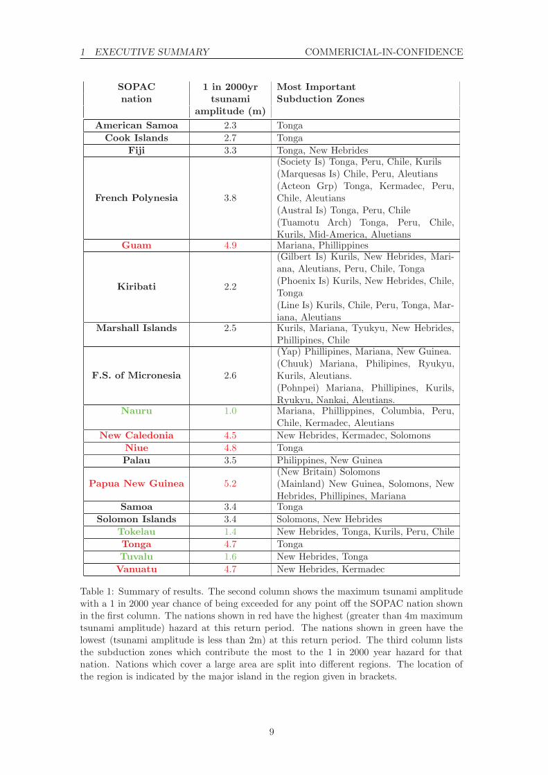
Table 1 shows the tsunami amplitude that has a 1 in 2000 year chance of beingexceeded for each SOPAC nation. Nations in red have the highest hazard at this returnperiod (Guam, New Caledonia, Niue, PNG, Tonga and Vanuatu), while those in greenhave the least (Nauru and Tuvalu). The other SOPAC nations are distributed betweenthese two more extreme groups.
Figure 2 shows the maximum amplitudes at the model output points for a returnperiod of 2000 years, along with those faults included in the study that lie in the mappedregion. It is clear from Figure 2 that most of the nations in the highest category mentionedabove lie very close to subduction zones. Typically where a nation is close to a subductionzone (the black lines in Figure 2) the bulk of the hazard to that nation comes from that zone.It should also be noted, that when an earthquake is that close to country, there is unlikelyto be enough time for an alert to reach that country from centralised warning centres suchas the Pacific Tsunami Warning Centre. Therefore public awareness campaigns are one ofthe best ways to reduce the hazard from such a local source.
When the nation is not close to any particular zone the hazard usually comes froma wider range of possible sources and is usually lower because the extra distance reducesthe amplitude of the tsunami by the time it reaches the nation concerned. These nationstypically have a more moderate hazard (e.g. French Polynesia). There would also be moretime for a warning from organisations such as the PTWC to reach those countries. Somenations (eg Nauru and Tuvalu) are not located optimally for any zone to send a tsunamitowards them and they thus experience relatively low tsunami hazard. Since some of
8
1 EXECUTIVE SUMMARY COMMERICIAL-IN-CONFIDENCE
SOPAC 1 in 2000yr Most Importantnation tsunami Subduction Zones
amplitude (m)American Samoa 2.3 Tonga
Cook Islands 2.7 TongaFiji 3.3 Tonga, New Hebrides
French Polynesia 3.8
(Society Is) Tonga, Peru, Chile, Kurils(Marquesas Is) Chile, Peru, Aleutians(Acteon Grp) Tonga, Kermadec, Peru,Chile, Aleutians(Austral Is) Tonga, Peru, Chile(Tuamotu Arch) Tonga, Peru, Chile,Kurils, Mid-America, Aluetians
Guam 4.9 Mariana, Phillippines
Kiribati 2.2
(Gilbert Is) Kurils, New Hebrides, Mari-ana, Aleutians, Peru, Chile, Tonga(Phoenix Is) Kurils, New Hebrides, Chile,Tonga(Line Is) Kurils, Chile, Peru, Tonga, Mar-iana, Aleutians
Marshall Islands 2.5 Kurils, Mariana, Tyukyu, New Hebrides,Phillipines, Chile
F.S. of Micronesia 2.6
(Yap) Phillipines, Mariana, New Guinea.(Chuuk) Mariana, Philipines, Ryukyu,Kurils, Aleutians.(Pohnpei) Mariana, Phillipines, Kurils,Ryukyu, Nankai, Aleutians.
Nauru 1.0 Mariana, Phillippines, Columbia, Peru,Chile, Kermadec, Aleutians
New Caledonia 4.5 New Hebrides, Kermadec, SolomonsNiue 4.8 TongaPalau 3.5 Philippines, New Guinea
Papua New Guinea 5.2(New Britain) Solomons(Mainland) New Guinea, Solomons, NewHebrides, Phillipines, Mariana
Samoa 3.4 TongaSolomon Islands 3.4 Solomons, New Hebrides
Tokelau 1.4 New Hebrides, Tonga, Kurils, Peru, ChileTonga 4.7 TongaTuvalu 1.6 New Hebrides, Tonga
Vanuatu 4.7 New Hebrides, Kermadec
Table 1: Summary of results. The second column shows the maximum tsunami amplitudewith a 1 in 2000 year chance of being exceeded for any point off the SOPAC nation shownin the first column. The nations shown in red have the highest (greater than 4m maximumtsunami amplitude) hazard at this return period. The nations shown in green have thelowest (tsunami amplitude is less than 2m) at this return period. The third column liststhe subduction zones which contribute the most to the 1 in 2000 year hazard for thatnation. Nations which cover a large area are split into different regions. The location ofthe region is indicated by the major island in the region given in brackets.
9

1 EXECUTIVE SUMMARY COMMERICIAL-IN-CONFIDENCE
the SOPAC nations are very spread out over the Pacific, the zones which are the mostimportant to that nation can vary significantly for different parts of the country. For amore detailed discussion for the hazard for each country, please see Section 3.
It is also important to emphasise that whether the risk (likelihood of damage ordeath) from a tsunami also depends on the density of infrastructure in low lying areasexposed to tsunami attack and the amount of warning received and the responses to it.For some countries, even if the tsunami hazard offshore is fairly low, the consequences ofthe event could potentially be high. Only more detailed modelling and analysis of eachspecific island could determine whether this indeed the case for any of the countries coveredby this report.
The other factor to bear in mind, is that the earthquake recurrence model usedin this assessment takes the return periods of smaller magnitude earthquakes that haveoccurred historically and extrapolates this to longer return periods to estimate the returnperiod of much larger earthquakes that haven’t happend historically. Therefore there ismuch more uncertainity in the hazard estimates at the longer return periods. Additionaldata, particularly palaeo-tsunami data, is required to reduce the uncertainity in the hazardestimates given here for the longer return periods. This uncertainity would be the largestfor countries whose main source of hazard comes from a zone which has not experienced avery large earthquake in the historic or known pre-historic catalogue. One example of thiswould be the Mariana’s subduction zone which has not experienced an earthquake largerthan 7.0-7.5 since 1900. The Mariana zone is an important source of hazard to islands suchas Guam.
1.5 Glossary
Amplitude Height of the crest of the tsunami wave above mean sea level.Bathymetry The measurement of the depth of the ocean floor from the
water surface.Probabilistic Tsunami HazardMap
This map shows the wave amplitude around the coast thathas a particular chance of being exceeded per annum. Thelarger the wave amplitude, the greater the hazard.
Run-up height The maximum water elevation within the limit of inunda-tion. It is usually greater than the wave amplitude at thecoast.
Subduction zone A region of the earth where two tectonic plates are converg-ing and one plate is sliding beneath the other. One exampleis the Sunda Arc that stretches from Timor to Burma.
Topography The measurement of the elevation of the land surface fromsea level.
Tsunami A wave created by a sudden disturbance of water. It is fastmoving and has a small amplitude in deep water, but slowsdown and increases in height as it reaches shallow water.
Tsunamigenic Capable of producing a tsunami.
10

2 INTRODUCTION TO TSUNAMI COMMERICIAL-IN-CONFIDENCE
2 Introduction to Tsunami
Tsunami are caused when large masses of water in the ocean are suddenly displaced bysome event. Gravity acts to return the displaced water to its equilibrium position and thedisturbance propagates as a wave, possibly for a very long distance. They differ from windgenerated waves in that their wavelengths (distance from peak to peak) are very large,exceeding 100 kilometres in the open ocean, they involve movement of the water all theway to the ocean floor, and they travel very quickly, of the order of 600 to 700 kilometresper hour or more in deep water. Even very significant tsunami will have amplitudes of onlya few tens of centimetres in deep water and are likely to pass unnoticed by the occupantsof a boat. However they carry a great deal of energy and they are able to transport thisenergy very long distances. When these waves reach shallow water they slow down and“bunch up” (their wavelength decreases), and their height increases dramatically, a processknown as shoaling. The maximum amplitude of the 2004 Boxing Day event was estimatedto be around 0.6 metres in the open ocean (Song et al, 2005) but the tsunami ran upto heights of ten metres along many coasts, even those thousands of kilometres from theearthquake (for example in India, see Narayan et al 2005).
The most common causes of tsunami are large earthquakes occurring under the seafloor, when the sudden movement of large slabs of rock causes the overlying column ofwater to be displaced. Submarine landslides also cause tsunami, when sediment on steepslopes becomes unstable and fails under gravity, displacing a large volume of water. Lesscommon are tsunami caused by the explosion or collapse of a volcano. Asteroids andcomets may also generate tsunami if they fall into the ocean and, although such eventsare rare, there is evidence that tsunami generated by this mechanism may have reachedAustralia in prehistoric times (Bryant, 2001).
2.1 Earthquake Sources
The most common causes of tsunami are earthquakes along oceanic subduction zones.Subduction zones occur where two tectonic plates are colliding, and one of the plates issliding (subducting) beneath the other (Figure 4). As this happens friction between the two
Figure 4: Mechanism for tsunami generation in an oceanic subduction zone.
plates may cause the upper plate to stick to the subducting plate and to become distortedby its motion. Eventually the stress associated with this deformation accumulates to suchan extent that it can no longer be sustained by the frictional force between the plates,resulting in a sudden movement of the upper plate as it springs back into place. This is
11
2 INTRODUCTION TO TSUNAMI COMMERICIAL-IN-CONFIDENCE
known as a subduction zone earthquake. This movement causes a sudden displacementof the water lying above the plate, producing a tsunami. Not all earthquakes occur insubduction zones, and other types of earthquakes have been responsible for generatingtsunami. However subduction zones have the potential to produce the largest earthquakesand the most significant tsunami. For this reason this study focuses exclusively on theoceanic subduction zones that could produce tsunami which impact on the area of interest.
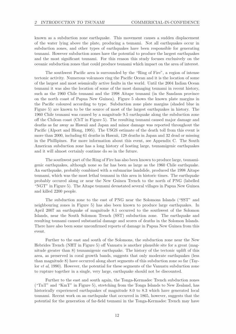
The southwest Pacific area is surrounded by the “Ring of Fire”, a region of intensetectonic activity. Numerous volcanoes ring the Pacific Ocean and it is the location of someof the largest and most seismically active faults in the world. Until the 2004 Indian Oceantsunami it was also the location of some of the most damaging tsunami in recent history,such as the 1960 Chile tsunami and the 1998 Aitape tsunami (in the Sandaun provinceon the north coast of Papua New Guinea). Figure 5 shows the known plate margins inthe Pacific coloured according to type. Subduction zone plate margins (shaded blue inFigure 5) are known to be the source of most of the largest earthquakes in history. The1960 Chile tsunami was caused by a magnitude 9.5 earthquake along the subduction zoneoff the Chilean coast (ChT in Figure 5). The resulting tsunami caused major damage anddeaths as far away as Hawaii and Japan and minor damage was reported throughout thePacific (Alport and Blong, 1995). The USGS estimate of the death toll from this event ismore than 2000, including 61 deaths in Hawaii, 128 deaths in Japan and 32 dead or missingin the Phillipines. For more information about this event, see Appendix C. The SouthAmerican subduction zone has a long history of hosting large, tsunamigenic earthquakesand it will almost certainly continue do so in the future.
The southwest part of the Ring of Fire has also been known to produce large, tsunami-genic earthquakes, although none so far has been as large as the 1960 Chile earthquake.An earthquake, probably combined with a submarine landslide, produced the 1998 Aitapetsunami, which was the most lethal tsunami in this area in historic times. The earthquakeprobably occured along or near the New Guinea Trench to the north of PNG (labelled“NGT” in Figure 5). The Aitape tsunami devastated several villages in Papua New Guineaand killed 2200 people.
The subduction zone to the east of PNG near the Solomons Islands (“SST” andneighbouring zones in Figure 5) has also been known to produce large earthquakes. InApril 2007 an earthquake of magnitude 8.1 occurred to the southwest of the SolomonIslands, near the South Solomon Trench (SST) subduction zone. The earthquake andresulting tsunami caused substantial damage and scores of deaths in the Solomon Islands.There have also been some unconfirmed reports of damage in Papua New Guinea from thisevent.
Further to the east and south of the Solomons, the subduction zone near the NewHebrides Trench (NHT in Figure 5) off Vanuatu is another plausible site for a great (mag-nitude greater than 8) tsunamigenic earthquake. The history of the tectonic uplift of thisarea, as preserved in coral growth bands, suggests that only moderate earthquakes (lessthan magnitude 8) have occurred along short segments of this subduction zone so far (Tay-lor et al, 1990). However, the potential for these segments of the Vanuatu subduction zoneto rupture together in a single, very large, earthquake should not be discounted.
Further to the east and south again, the Tonga-Kermadec Trench subduction zones(“TnT” and “KmT” in Figure 5), stretching from the Tonga Islands to New Zealand, hashistorically experienced earthquakes of magnitude 8.0 to 8.3 which have generated localtsunami. Recent work on an earthquake that occurred in 1865, however, suggests that thepotential for the generation of far-field tsunami in the Tonga-Kermadec Trench may have
12
2 INTRODUCTION TO TSUNAMI COMMERICIAL-IN-CONFIDENCE
120˚ 140˚ 160˚ 180˚ 200˚ 220˚ 240˚ 260˚ 280˚ 300˚
−60˚
−40˚
−20˚
0˚
20˚
40˚
60˚
PyT
TnT
KmT
HkT
NHTSST
AlTCsT
MAT
PrT
ChT
KrT
JpT
NaT IBT
MnT
RyT
PhTNGT
ShT
aT
CoT
Continental Rift Oceanic SpreadingContinental Transform Oceanic TransformContinental Convergent Oceanic ConvergentSubduction Zone
Figure 5: Map of major plate boundaries from Bird (2002). All subductions zones shown (in blue)were included in the study, and are labelled: AlT - Aleutian Trench, ChT - Chile Trench, CoT -Columbia Trench, CsT - Cascadia Trough, HkT - Hikurangi Trough, IBT - Izu-Bonin Trench, JpT- Japan Trench, KmT - Kermadec Trench, KrT - Kuril Trench, MnT - Mariana Trench, MAT -Middle America Trench, NaT - Nankai Trough, NGT - New Guinea Trench, NHT - New HebridesTrench, PhT - Philippines Trench, PrT - Peru Trench, PyT - Puysegur Trench, RyT - RyukyuTrench, SaT - South Sandwich Trench, SST - South Solomons Trench, TnT - Tonga Trench.
been underestimated (Okal et al, 2004).
South of New Zealand, much of the relative plate motion is in the strike direction(that is, in the direction of the fault line), so that even when large earthquakes occur thevertical component of the slip is small and they typically generate only small tsunami.There is, however, a section of plate boundary just to the south of New Zealand knownas the Puysegur Trench (“PyT” in Figure 5), along which subduction has been occurringfor the past ten million years, a very short time in geologic terms (Meckel et al, 2005).Subduction zones with such short histories are rare and their potential to produce largeearthquakes and tsunami is unknown. No major tsunamigenic earthquake has occurred onthis trench in the historic past (greater than magnitude 8), which would suggest either thatsubduction is mostly aseismic and no large earthquakes will occur, or that the subductionzone has been accumulating strain energy for over 200 years and has the potential to rupturein a major earthquake. However, the magnitude 7.4 earthquake along the Puysegur zone inSeptember 2007 did create a small tsunami which was detectable by a deep ocean pressuregauge just off the fault (Bathgate et al, 2008).
13

2 INTRODUCTION TO TSUNAMI COMMERICIAL-IN-CONFIDENCE
In the north Pacific, the subduction zone off Cascadia (“CsT” in Figure 5) is thoughtto have hosted an earthquake around magnitude 9 in 1700 which generated a large tsunamithat impacted Japan (Atwater et al, 2005). More recently, large earthquakes along theAleutian Islands subduction zone (“AlT” in Figure 5) have generated waves that weredamaging as far as Hawaii. The 1964 Prince William Sound earthquake (magnitude 9.2)created a damaging tsunami in Alaska. According to the USGS, that event took 125lives (110 from the tsunami and 15 from the earthquake). There were also tsunamigenicevents in 1965 (the magnitude 8.7 Rat Islands earthquake) and 1957 (the magnitude 8.6Andreanof Islands earthquake). Both were large enough to create damaging tsunami inthe Alaskan region.
Japan has a record of seismicity going back nearly one thousand years from thesubduction zones off its coast. Events along the Nankai (“NaT”) and Kamchatka-Kurilszones (“KrT”) are known to create very large local tsunami, but as yet this area has notexperienced any earthquake that we can be confident had a magnitude of 9 or above.
In summary, there are major subduction zones in the west, north and east of thePacific Ocean basin that either have produced damaging tsunami in the past or couldplausibly produce them in the future. Therefore there is a real prospect that any of thenations in the southwest Pacific might be exposed to a significant tsunami hazard.
2.1.1 Other Tsunamigenic Mechanisms
Subduction zone earthquakes are not the only possible sources of tsunami. As mentionedabove, the Pacific is rimmed with volcanoes, many of which are submarine or near thecoast. Should one of these volcanoes erupt violently or collapse suddenly into the sea,there is a real prospect of it producing a tsunami. For example, in 1888 a large tsunami,caused by the flank collapse of Mount Ritter in Papua New Guinea, ran up to 12 – 15metres and wiped out villages on the western coast of New Britain (Johnson, 1987). Theprobability of this occurring is difficult to estimate without detailed study of the volcanoesconcerned and may be a topic for future work.
The Aitape tsunami demonstrated that there is also the prospect of a landslide sourcegenerating a tsunami. The largest tsunami in history occurred in 1958 when an earthquaketriggered a landslide into the Lituya Bay fjord in Alaska. The tsunami reached an altitudeof 510 metres on the other side of the bay (Mader, 2002). However, tsunami generated infjords usually remain trapped within them and are rarely considered to be a major threatoutside of the local region.
Submarine landslides on the continental slope are also a genuine hazard. These canbe triggered by a nearby earthquake, or may happen without warning. Historically theyhave tended to produce large, but local tsunami (for example the 1998 Aitape and 1953Suva tsunami) but there is the prospect of a major tsunami that impacts the far-field ifthe landslide is sufficiently large. Again, this may be a topic for future work.
The largest tsunami of all are likely to be generated by asteroid impacts. It isknown that major extinction events marking the transitions between geologic eras, such asthat between the Cretaceous and Tertiary periods 65 million years ago, are the result ofmassive impacts of comets or asteroids of about ten kilometres in diameter. Objects capableof causing worldwide catastrophes are most certainly associated with massive tsunami,with wave amplitudes far exceeding any tsunami in historic times. There is considerableuncertainty about the generation and propagation of tsunami waves from intermediate-
14

2 INTRODUCTION TO TSUNAMI COMMERICIAL-IN-CONFIDENCE
sized objects with diameters in the range 100 metres to one kilometre. Smaller objectsalmost certainly do not generate tsunami. Larger objects are clearly capable of penetratingto the ocean floor and generating long-period waves that travel across the ocean with littleloss of energy. These are likely to be quite rare, but potentially devastating, events.
15

3 RESULTS COMMERICIAL-IN-CONFIDENCE
3 Results
This section consists of discussions of the results as they apply to each SOPAC nationincluded in the study. The diagrams presented in this section have been limited to hazardcurves for return periods of between 10 and 2000 years, and maximum amplitude excee-dence and regional weighted deaggregated hazard maps at 2000 year return periods. Forsome nations the results have been further divided, either because of geographic spread,or because different regions have significantly different hazard profiles.
In each section there will be one figure containing three hazard maps for that region.Part (a) shows the hazard curves, (b) the regional weighted deaggregated hazard map and(c) is the maximum amplitude map for the 2000 year return period. For a more detailedexplanation of the maps, please see Section 1.3.
The diagrams and discussion in this section can only give an overview of the magni-tude and source of the hazard faced by each nation. The maximum amplitude maps arerestricted to a 2000 year return period, and the regional weighted deaggregated hazardmaps only give a general idea of the source of the hazard for the region as a whole. TheKML files on the accompanying DVD can be used to gain a more detailed picture of thehazard of each nation. For example, if one is interested in the source of the hazard at aparticular location one should look on the accompanying DVD for a deaggregated hazardmap drawn for a model output point close to that location.
In each section, we also briefly mention whether there were any recorded effects ofthe 1960 Chile tsunami on the country. This information should be only taken as a guide tothe possible effects of large tsunami on that nation. The details of the inundation dependcritically on the direction and earthquake source properties and can vary from tsunamito tsunami. The amount of information on the effects of the 1960 Chile tsunami is alsobiased towards locations where we have extant records of the impact of the tsunami. Someislands may be more severely impacted by this event in specific areas, but the sources weconsulted may not have included that information. For a summary of all the informationconcerning the 1960 tsunami, see Appendix C.
16
3 RESULTS COMMERICIAL-IN-CONFIDENCE
3.1 American Samoa
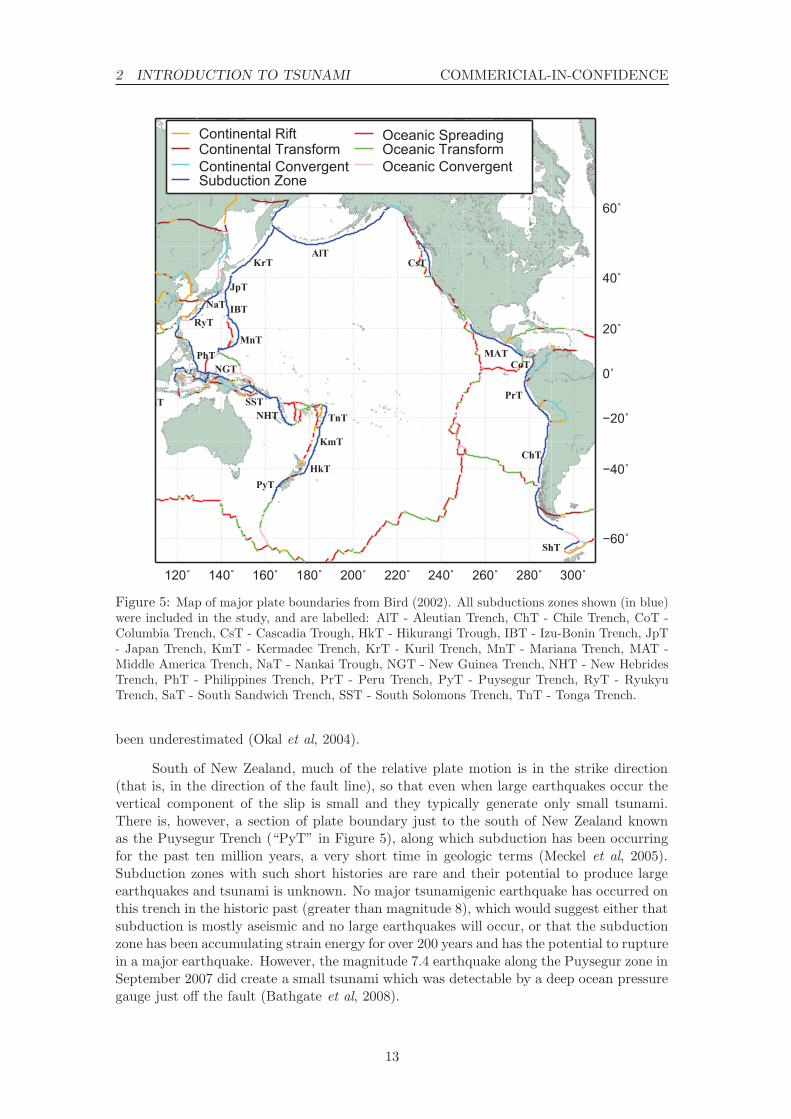
The hazard profile of American Samoa separates neatly between Swain’s Atoll and themain islands of Tutuila, Aunuu, Ofu, Olosega and Tau. Figure 6(a) shows that maximumamplitudes (in 100 metres of water) for a 100 year return period are approximately 20centimetres at Swain’s Atoll and 30 to 40 centimetres near the main islands, rising fora 2000 year return period to around 90 centimetres and 2.2 metres respectively (see alsoFigure 6(c)). Figure 6(b) shows that the hazard at the 2000 year return period is dominatedby the Tonga trench, as is to be expected given its proximity.
The tsunami generated by the 1960 Chile earthquake reached a maximum run-upheight of over three metres at Pago Pago village on Tutuila island (Allport and Blong,1995). Buildings were moved off their foundations and a house washed into the bay. Noloss of life was reported. Note that the most of the 1 in 2000 year hazard to AmericanSamoa comes from sources to the west of the islands. Therefore any tsunami from thosesources may affect American Samoa quite different to the 1960 tsunami.
0.02
0.050.10.2
0.512
5
Max
Tsu
nam
i Am
plitu
de (m
)
10 20 50 100 200 500 1000 2000
Mean Return Period (years)
(a)
120˚ 150˚ 180˚ 210˚ 240˚ 270˚ 300˚ −60˚−30˚
0˚30˚
60˚
5%10
%15
%
0 15Percentage Weighted Contribution
(b)
190˚
−14˚
−12˚
0.7 2.3
Maximum Amplitude (metres)
Tutuila
Aunuu
Swains Atoll
Ofu Olosega
Tau
(c)
Figure 6: American Samoa:- (a) Hazard curves for all model output points. (b) Regional weighteddeaggregated hazard. (c) Maximum amplitude at a 2000 year return period for all model outputpoints.
17

3 RESULTS COMMERICIAL-IN-CONFIDENCE
3.2 The Cook Islands
The hazard at the 2000 year return period for the northern Cook Islands (latitude greaterthan -15◦) is lower than that for the southern islands. This is clearly the result of thelocation and orientation of the most significant source of tsunamegenic earthquakes forthis nation, the Tonga trench, which extends northwards only to about -15◦, and whichis oriented so as to direct most tsunami energy south of the northern group of islands(Figure 5). The 2000 year maximum amplitudes are of the order of 1.7 metres for thenorthern islands and up to 2.8 metres in parts of the southern group (Figure 7(c)), whilethe 100 year maximum amplitudes range from about 0.3 to 0.4 metres (Figure 7(a)). Atthe 2000 year amplitude level the hazard is dominated by the Tonga trench (Figure7(b)).
0.02
0.050.10.2
0.512
5
Max
Tsu
nam
i Am
plitu
de (m
)
10 20 50 100 200 500 1000 2000
Mean Return Period (years)
(a)
120˚ 150˚ 180˚ 210˚ 240˚ 270˚ 300˚ −60˚−30˚
0˚30˚
60˚
2%4%
6%8%
0.0 6.8Percentage Weighted Contribution
(b)
195˚ 200˚
−20˚
−15˚
−10˚
1.1 2.8
Maximum Amplitude (metres)
Palmerston Island
Penrhyn
Mangaia
Suwarro
Rarotonga
(c)
Figure 7: Cook Islands:- (a) Hazard curves for all model output points. (b) Regional weighteddeaggregated hazard. (c) Maximum amplitude at a 2000 year return period for all model outputpoints.
18

3 RESULTS COMMERICIAL-IN-CONFIDENCE
3.3 Fiji
As Figure 8(b) shows, the hazard at the 2000 year return period is dominated by theTonga trench, with some contribution from the New Hebrides trench. This is reflected inthe maximum amplitudes at the 2000 year return period (Figure 8(c)), which range from1 to 3.3 metres with the amplitudes in the eastern islands and on the eastern coast ofVanua Levu being significantly higher than elsewhere. For a return period of 100 years themaximum amplitudes range from 0.2 to 0.6 metres. In Fiji reports of the 1960 tsunamiappear to be confined to the effects in Suva harbour. The maximum runup was reportedto be about 0.5 metres, and the tsunami induced a powerful surge in the harbour. Manyboats sustained damage, but no loss of life was recorded (Allport and Blong, 1995). Aswith American Samoa, the direction of this wave is quite different from the zones thatcontribute the most to the 1 in 2000 year tsunami hazard.
0.02
0.050.10.2
0.512
5
Max
Tsu
nam
i Am
plitu
de (m
)
10 20 50 100 200 500 1000 2000
Mean Return Period (years)
(a)
120˚ 150˚ 180˚ 210˚ 240˚ 270˚ 300˚−60˚
−30˚
0˚
30˚
60˚
5%
0.0 4.5Percentage Weighted Contribution
(b)
176˚ 178˚ 180˚ 182˚
−20˚
−18˚
−16˚
−14˚
−12˚
1.1 3.3
Maximum Amplitude (metres)
Rotuma
Viti Levu
Vanua Levu
(c)
Figure 8: Fiji:- (a) Hazard curves for all model output points. (b) Regional weighted deaggregatedhazard. (c) Maximum amplitude at a 2000 year return period for all model output points.
19

3 RESULTS COMMERICIAL-IN-CONFIDENCE
3.4 French Polynesia
3.4.1 French Polynesia: The Society Islands
The major contribution to the hazard of the Society Islands (2000 year return period)comes from the Tonga trench (Figure 9(b)). Some hazard also comes from the Peru, Chileand Kurils subduction zones. The major islands can expect maximum amplitudes at the2000 year return period of around 2 metres (Figure 9(c)). The maximum amplitudes at a100 year return period are much smaller, of the order of 0.2 to 0.5 metres (Figure 9(a)).
In French Polynesia many of the islands are protected by outer reefs and deep lagoonsfrom the effects of the 1960 tsunami, with rather steep bathymetry offshore, and in mostcases only slight damage was sustained. No loss of life was recorded throughout the islands.The average runup surveyed in Tahiti was 1.7 metres. Larger runups, up to 3.4 metres,were recorded along the north shore of the island which is more exposed to the open ocean(Vitousek, 1963).
0.02
0.050.10.2
0.512
5
Max
Tsu
nam
i Am
plitu
de (m
)
10 20 50 100 200 500 1000 2000
Mean Return Period (years)
(a)
120˚ 150˚ 180˚ 210˚ 240˚ 270˚ 300˚ −60˚−30˚
0˚30˚
60˚
1%2%
3%4%
0.0 3.5Percentage Weighted Contribution
(b)
208˚ 210˚−18˚
−17˚
−16˚
0.9 2.1
Maximum Amplitude (metres)
Bora Bora
Tahaa
Raiatea Huahine
Tahiti
(c)
Figure 9: French Polynesia: Society Islands:- (a) Hazard curves for all model output points. (b)Regional weighted deaggregated hazard. (c) Maximum amplitude at a 2000 year return period forall model output points.
20

3 RESULTS COMMERICIAL-IN-CONFIDENCE
3.4.2 French Polynesia: The Marquesas Islands
The large 2000 year maximum amplitude (≈ 3.8 metres) computed at one model outputpoint on Hiva Oa (Figure 10(c) and the uppermost curve in Figure 10(a)) should be in-terpreted with caution; it may be a real effect or it may be an artefact of the complexbathymetry in the region. A more detailed study of this part of the coast would be re-quired to clarify this. Regardless of this, Figure 10(c) indicates 2000 year amplitudes ofabout 2.6 metres off Nuku Hiva and at least 2.8 metres off Hiva Oa. At a return periodof 100 years the maximum amplitudes over the region vary from around 0.3 to 0.7 metres.The major contributors to the hazard for this region at a 2000 year return period are thenorthern part of the Chile trench, and the southern part of the Peru trench (Figure 10(b)).
The greatest effects in French Polynesia from the 1960 tsunami were felt in the Mar-quesas Islands which have few outer reefs and more gradual changes in offshore bathymetry.Runups of at least 4.5 metres (possibly up to nine metres) were observed. Destruction ofbuildings near the shore was reported (Vitousek, 1963).
0.02
0.050.10.2
0.512
5
Max
Tsu
nam
i Am
plitu
de (m
)
10 20 50 100 200 500 1000 2000
Mean Return Period (years)
(a)
120˚ 150˚ 180˚ 210˚ 240˚ 270˚ 300˚−60˚
−30˚0˚30˚
60˚
1%2%
3%
0.0 2.5Percentage Weighted Contribution
(b)
220˚
−10˚
−8˚
1.4 3.8
Maximum Amplitude (metres)
Eiao
Nuku Hiva
Ua PouHiva Oa
Fatu Hiva
(c)
Figure 10: French Polynesia: Marquesas Islands:- (a) Hazard curves for all model output points.(b) Regional weighted deaggregated hazard. (c) Maximum amplitude at a 2000 year return periodfor all model output points.
21

3 RESULTS COMMERICIAL-IN-CONFIDENCE
3.4.3 French Polynesia: The Acteon Group, Gambier Islands and southeastTuamotu Archipelago
Maximum amplitudes at a 2000 year return period of up to 2.3 metres were computednear Mururoa, 2.5 metres near the Acteon Group, 2.2 metres near Marutea and 2.0 metresnear the Gambier Islands (Figure 11(c)). For a return period of 100 years the maximumamplitudes ranged from about 0.3 to 0.5 metres over the region as a whole. The majorsource of hazard for the region at a 2000 year return period was the Tonga trench, withsignificant contributions from the Kermadec, Peru and Chile trenches (Figure 11(b)).
0.02
0.050.10.2
0.512
5
Max
Tsu
nam
i Am
plitu
de (m
)
10 20 50 100 200 500 1000 2000
Mean Return Period (years)
(a)
120˚ 150˚ 180˚ 210˚ 240˚ 270˚ 300˚−60˚
−30˚0˚30˚
60˚
1%2%
3%
0.0 2.1Percentage Weighted Contribution
(b)
220˚ 222˚ 224˚−24˚
−22˚
−20˚
1.4 2.5
Maximum Amplitude (metres)
Tematagi
Tureia
Mururoa Acteon GroupMarutea
Gambier Islands
(c)
Figure 11: French Polynesia: The Acteon Group, Gambier Islands and southeast TuamotuArchipelago:- (a) Hazard curves for all model output points. (b) Regional weighted deaggregatedhazard. (c) Maximum amplitude at a 2000 year return period for all model output points.
22

3 RESULTS COMMERICIAL-IN-CONFIDENCE
3.4.4 French Polynesia: The Austral Islands
The 2000 year maximum amplitudes are uniformly of the order of 1.5 to 2 metres acrossthe Austral Islands at a 2000 year return period, and 0.3 to 0.4 metres at a 100 year returnperiod (Figure 12(a)). The dominant source of hazard for the region is the Tonga trench(Figure 12(b)).
0.02
0.050.10.2
0.512
5
Max
Tsu
nam
i Am
plitu
de (m
)
10 20 50 100 200 500 1000 2000
Mean Return Period (years)
(a)
120˚ 150˚ 180˚ 210˚ 240˚ 270˚ 300˚ −60˚−30˚
0˚30˚
60˚
1%2%
3%4%
5%0.0 4.2Percentage Weighted Contribution
(b)
210˚ 215˚
−25˚
1.6 2.0
Maximum Amplitude (metres)
RimataraRuruta
Mataura
Rapa
Raivavae
(c)
Figure 12: French Polynesia: The Austral Islands:- (a) Hazard curves for all model output points.(b) Regional weighted deaggregated hazard. (c) Maximum amplitude at a 2000 year return periodfor all model output points.
23

3 RESULTS COMMERICIAL-IN-CONFIDENCE
3.4.5 French Polynesia: The Tuamotu Archipelago
Maximum amplitudes of the order of 2 to 3 metres were computed in the northeasternand southwestern parts of the archipelago, particularly around Kaukura and Reao (Fig-ure 13(c)). For a return period of 100 years maximum amplitudes of 0.5 to 0.6 metres canbe expected throughout much of the archipelago. The hazard for the region at a 2000 yearreturn period originates from the Tonga, Peru and Chile trenches(Figure 13(b)).
0.02
0.050.10.2
0.512
5
Max
Tsu
nam
i Am
plitu
de (m
)
10 20 50 100 200 500 1000 2000
Mean Return Period (years)
(a)
120˚ 150˚ 180˚ 210˚ 240˚ 270˚ 300˚−60˚
−30˚0˚30˚
60˚
1%2%
0.0 1.1Percentage Weighted Contribution
(b)
212˚ 214˚ 216˚ 218˚ 220˚ 222˚ 224˚
−20˚
−18˚
−16˚
−14˚
0.9 3.1
Maximum Amplitude (metres)
Kaukura
PukaruhaReao
(c)
Figure 13: French Polynesia: The Tuamotu Archipelago:- (a) Hazard curves for all model outputpoints. (b) Regional weighted deaggregated hazard. (c) Maximum amplitude at a 2000 year returnperiod for all model output points.
24
3 RESULTS COMMERICIAL-IN-CONFIDENCE
3.5 Guam
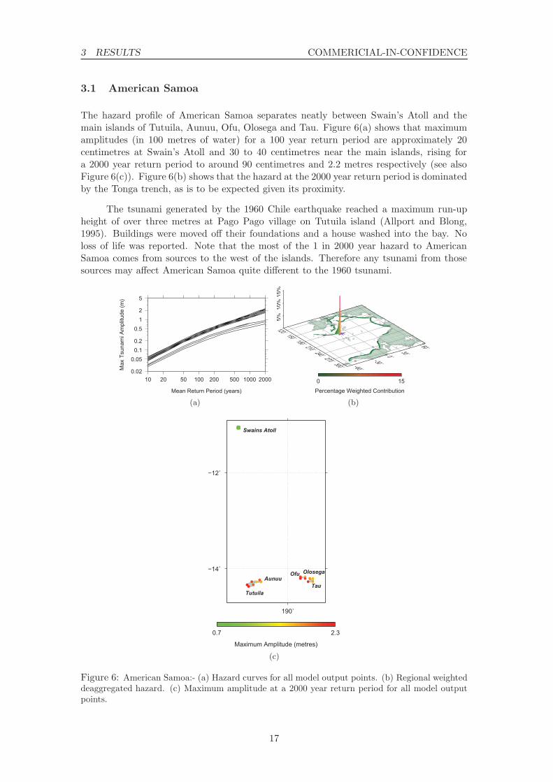
The Mariana trench lies close to Guam, to the south and east, and the highest amplitudesfor a 2000 year return period, up to 4.9 metres, are expected off the southern and easterncoasts (Figure 14(c)). For a 100 year return period the maximum amplitudes are of theorder of 0.5 to 0.6 metres for all model output points (Figure 14(a)). Figure 14(b) showsthat in addition to the Mariana trench, the Philippines Trench is also a significant sourceof hazard at a 2000 year return period.
0.02
0.050.10.2
0.512
5
Max
Tsu
nam
i Am
plitu
de (m
)
10 20 50 100 200 500 1000 2000
Mean Return Period (years)
(a)
120˚ 150˚ 180˚ 210˚ 240˚ 270˚ 300˚−60˚
−30˚0˚30˚
60˚
2%4%
0.0 4.4Percentage Weighted Contribution
(b)
144˚36' 144˚54'
13˚30'
3.0 4.9
Maximum Amplitude (metres)(c)
Figure 14: Guam:- (a) Hazard curves for all model output points. (b) Regional weighted deaggre-gated hazard. (c) Maximum amplitude at a 2000 year return period for all model output points.
25

3 RESULTS COMMERICIAL-IN-CONFIDENCE
3.6 Kiribati
3.6.1 Kiribati: The Gilbert Islands
Over much of the of the Gilbert Islands maximum amplitudes for a 2000 year return periodwere computed to be of the order of 1.0 to 1.4 metres, with generally lower amplitudesin the most southerly islands (Figure 15(c)). At a return period of 100 years maximumamplitudes of the order of 0.3 to 0.4 metres were typical. Figure 15(b) shows most of thehazard originating in the Kurils and New Hebrides trenches, with smaller contributionsfrom the Mariana, Aleutians, Peru, Chile and Tonga trenches.
0.02
0.050.10.2
0.512
5
Max
Tsu
nam
i Am
plitu
de (m
)
10 20 50 100 200 500 1000 2000
Mean Return Period (years)
(a)
120˚ 150˚ 180˚ 210˚ 240˚ 270˚ 300˚ −60˚−30˚
0˚30˚
60˚1%
2%
0.0 1.4Percentage Weighted Contribution
(b)
174˚ 176˚
−2˚
0˚
2˚
4˚
0.8 1.4
Maximum Amplitude (metres)
Butaritari
Tarawa
Arorae
Tabiteuea
(c)
Figure 15: Kiribati: Gilbert Islands:- (a) Hazard curves for all model output points. (b) Regionalweighted deaggregated hazard. (c) Maximum amplitude at a 2000 year return period for all modeloutput points.
26

3 RESULTS COMMERICIAL-IN-CONFIDENCE
3.6.2 Kiribati: The Phoenix Islands
Figure 16(a) shows that the maximum amplitudes at all return periods from 10 to 2000years are quite uniform over the model output points in the Phoenix Islands, with a max-imum amplitude of the order of one metre for a 2000 year return period, and 0.2 to 0.3metres for a 100 year return period. The origin of the hazard at a 2000 year return periodfor this region is predominantly the Kurils trench with smaller contributions from the NewHebrides trench, and the Chile trench (Figure 16(b)). Despite its proximity, the Tongatrench contributes little to the hazard because its orientation serves to direct tsunamienergy south of the Phoenix Islands.
0.02
0.050.10.2
0.512
5
Max
Tsu
nam
i Am
plitu
de (m
)
10 20 50 100 200 500 1000 2000
Mean Return Period (years)
(a)
120˚ 150˚ 180˚ 210˚ 240˚ 270˚ 300˚ −60˚−30˚
0˚30˚
60˚1%
2%3%
0.0 2.1Percentage Weighted Contribution
(b)
188˚
−4˚
0.9 1.3
Maximum Amplitude (metres)
Enderbury
Canton
ManraOrona
(c)
Figure 16: Kiribati: Phoenix Islands:- (a) Hazard curves for all model output points. (b) Regionalweighted deaggregated hazard. (c) Maximum amplitude at a 2000 year return period for all modeloutput points.
27
3 RESULTS COMMERICIAL-IN-CONFIDENCE
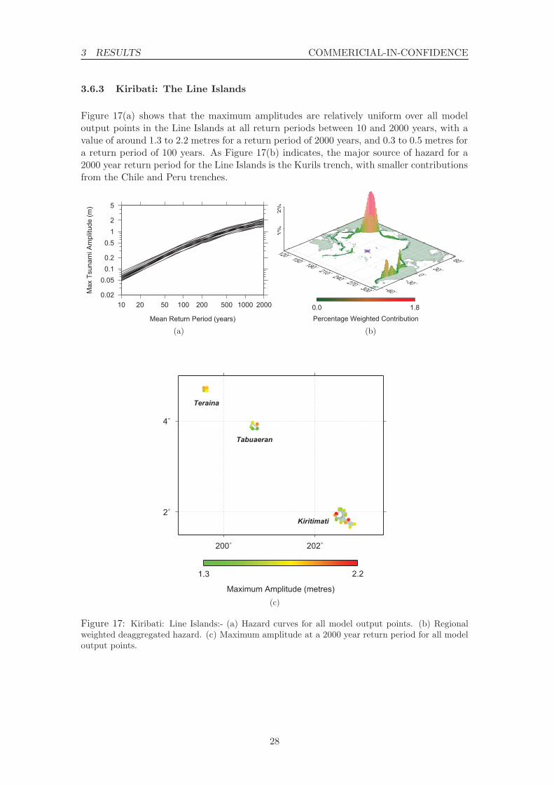
3.6.3 Kiribati: The Line Islands
Figure 17(a) shows that the maximum amplitudes are relatively uniform over all modeloutput points in the Line Islands at all return periods between 10 and 2000 years, with avalue of around 1.3 to 2.2 metres for a return period of 2000 years, and 0.3 to 0.5 metres fora return period of 100 years. As Figure 17(b) indicates, the major source of hazard for a2000 year return period for the Line Islands is the Kurils trench, with smaller contributionsfrom the Chile and Peru trenches.
0.02
0.050.10.2
0.512
5
Max
Tsu
nam
i Am
plitu
de (m
)
10 20 50 100 200 500 1000 2000
Mean Return Period (years)
(a)
120˚ 150˚ 180˚ 210˚ 240˚ 270˚ 300˚ −60˚−30˚
0˚30˚
60˚
1%2%
0.0 1.8Percentage Weighted Contribution
(b)
200˚ 202˚
2˚
4˚
1.3 2.2
Maximum Amplitude (metres)
Teraina
Tabuaeran
Kiritimati
(c)
Figure 17: Kiribati: Line Islands:- (a) Hazard curves for all model output points. (b) Regionalweighted deaggregated hazard. (c) Maximum amplitude at a 2000 year return period for all modeloutput points.
28
3 RESULTS COMMERICIAL-IN-CONFIDENCE
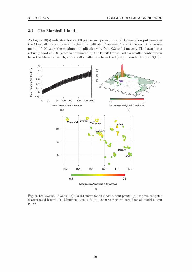
3.7 The Marshall Islands
As Figure 18(a) indicates, for a 2000 year return period most of the model output points inthe Marshall Islands have a maximum amplitude of between 1 and 2 metres. At a returnperiod of 100 years the maximum amplitudes vary from 0.2 to 0.4 metres. The hazard at areturn period of 2000 years is dominated by the Kurils trench, with a smaller contributionfrom the Mariana trench, and a still smaller one from the Ryukyu trench (Figure 18(b)).
0.02
0.050.10.2
0.512
5
Max
Tsu
nam
i Am
plitu
de (m
)
10 20 50 100 200 500 1000 2000
Mean Return Period (years)
(a)
120˚ 150˚ 180˚ 210˚ 240˚ 270˚ 300˚−60˚
−30˚
0˚30˚
60˚
1%2%
3%
0.0 2.7Percentage Weighted Contribution
(b)
162˚ 164˚ 166˚ 168˚ 170˚ 172˚
6˚
8˚
10˚
0.8 2.5
Maximum Amplitude (metres)
Mili
Majuro
PikinniEnewetakAiluk
Kwajalein
Rongelap
(c)
Figure 18: Marshall Islands:- (a) Hazard curves for all model output points. (b) Regional weighteddeaggregated hazard. (c) Maximum amplitude at a 2000 year return period for all model outputpoints.
29
3 RESULTS COMMERICIAL-IN-CONFIDENCE
3.8 The Federated States of Micronesia
The Federated States of Micronesia have a large east - west extent and are best treated inthree regions:
1. Yap State
2. Chuuk State
3. Pohnpei and Kosrae
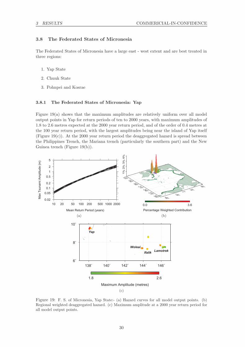
3.8.1 The Federated States of Micronesia: Yap
Figure 19(a) shows that the maximum amplitudes are relatively uniform over all modeloutput points in Yap for return periods of ten to 2000 years, with maximum amplitudes of1.8 to 2.6 metres expected at the 2000 year return period, and of the order of 0.4 metres atthe 100 year return period, with the largest amplitudes being near the island of Yap itself(Figure 19(c)). At the 2000 year return period the deaggregated hazard is spread betweenthe Philippines Trench, the Mariana trench (particularly the southern part) and the NewGuinea trench (Figure 19(b)).
0.02
0.050.10.2
0.512
5
Max
Tsu
nam
i Am
plitu
de (m
)
10 20 50 100 200 500 1000 2000
Mean Return Period (years)
(a)
120˚ 150˚ 180˚ 210˚ 240˚ 270˚ 300˚ −60˚−30˚
0˚30˚
60˚
1%2%
3%4%
0.0 3.6Percentage Weighted Contribution
(b)
138˚ 140˚ 142˚ 144˚ 146˚6˚
8˚
10˚
1.8 2.6
Maximum Amplitude (metres)
Yap
Woleai
Ifalik Lamotrek
(c)
Figure 19: F. S. of Micronesia, Yap State:- (a) Hazard curves for all model output points. (b)Regional weighted deaggregated hazard. (c) Maximum amplitude at a 2000 year return period forall model output points.
30
3 RESULTS COMMERICIAL-IN-CONFIDENCE
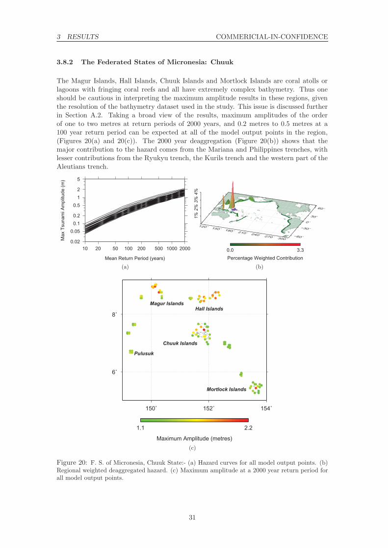
3.8.2 The Federated States of Micronesia: Chuuk
The Magur Islands, Hall Islands, Chuuk Islands and Mortlock Islands are coral atolls orlagoons with fringing coral reefs and all have extremely complex bathymetry. Thus oneshould be cautious in interpreting the maximum amplitude results in these regions, giventhe resolution of the bathymetry dataset used in the study. This issue is discussed furtherin Section A.2. Taking a broad view of the results, maximum amplitudes of the orderof one to two metres at return periods of 2000 years, and 0.2 metres to 0.5 metres at a100 year return period can be expected at all of the model output points in the region,(Figures 20(a) and 20(c)). The 2000 year deaggregation (Figure 20(b)) shows that themajor contribution to the hazard comes from the Mariana and Philippines trenches, withlesser contributions from the Ryukyu trench, the Kurils trench and the western part of theAleutians trench.
0.02
0.050.10.2
0.512
5
Max
Tsu
nam
i Am
plitu
de (m
)
10 20 50 100 200 500 1000 2000
Mean Return Period (years)
(a)
120˚ 150˚ 180˚ 210˚ 240˚ 270˚ 300˚−60˚
−30˚
0˚
30˚
60˚
1%2%
3%4%
0.0 3.3Percentage Weighted Contribution
(b)
150˚ 152˚ 154˚
6˚
8˚
1.1 2.2
Maximum Amplitude (metres)
Hall Islands
Chuuk Islands
Magur Islands
Pulusuk
Mortlock Islands
(c)
Figure 20: F. S. of Micronesia, Chuuk State:- (a) Hazard curves for all model output points. (b)Regional weighted deaggregated hazard. (c) Maximum amplitude at a 2000 year return period forall model output points.
31

3 RESULTS COMMERICIAL-IN-CONFIDENCE
3.8.3 Federated States of Micronesia: Pohnpei and Kosrae
Maximum amplitudes for a 2000 year return period vary from 1.1 to 1.9 metres, with thehighest values being computed in Oroluk and Pohnpei (Figure 21(c)). At a return periodof 100 years the maximum amplitudes vary from around 0.2 to 0.4 metres. Figure 21(b)indicates that, in common with Chuuk, the greatest contribution to the hazard in thisregion is made by the Mariana and Philippines faults, with significant contributions fromthe Kurils trench, the Ryukyu and Nankai trenches and to a lesser extent the western partof the Aleutians trench.
0.02
0.050.10.2
0.512
5
Max
Tsu
nam
i Am
plitu
de (m
)
10 20 50 100 200 500 1000 2000
Mean Return Period (years)
(a)
120˚ 150˚ 180˚ 210˚ 240˚ 270˚ 300˚−60˚
−30˚
0˚
30˚
60˚
1%2%
3%
0.0 2.9Percentage Weighted Contribution
(b)
156˚ 158˚ 160˚ 162˚
6˚
8˚
1.1 1.9
Maximum Amplitude (metres)
Oroluk
Pohnpei
Ngatik
Pingelap
Kosrae
(c)
Figure 21: F. S. of Micronesia, Pohnpei and Kosrae:- (a) Hazard curves for all model outputpoints. (b) Regional weighted deaggregated hazard. (c) Maximum amplitude at a 2000 year returnperiod for all model output points.
32

3 RESULTS COMMERICIAL-IN-CONFIDENCE
3.9 Nauru
Nauru has a relatively low hazard, with maximum amplitudes at all model output pointscomputed at about 1 metre for a return period of 2000 years and about 0.2 metres for areturn period of 100 years (Figure 22(a)). Figure 22(b) shows that for a 2000 year returnperiod the hazard originates predominantly from the Solomons, New Hebrides and Kurilstrenches, with smaller contributions from the Mariana, Philippines and Peru Trenches.
0.02
0.050.10.2
0.512
5
Max
Tsu
nam
i Am
plitu
de (m
)
10 20 50 100 200 500 1000 2000
Mean Return Period (years)
(a)
120˚ 150˚ 180˚ 210˚ 240˚ 270˚ 300˚ −60˚−30˚
0˚30˚
60˚
1%2%
0.0 1.9Percentage Weighted Contribution
(b)
0.9 1.0
Maximum Amplitude (metres)(c)
Figure 22: Nauru:- (a) Hazard curves for all model output points. (b) Regional weighted deaggre-gated hazard. (c) Maximum amplitude at a 2000 year return period for all model output points.
33

3 RESULTS COMMERICIAL-IN-CONFIDENCE
3.10 New Caledonia
The hazard for New Caledonia originates predominantly from the New Hebrides trench(Figure 23(b)), which lies close to the northeast (the black line in Figure 23(c)). Con-sequently the maximum amplitudes are somewhat greater on the northeastern coastlinesof the islands, with values of up to 4.5 metres, while maximum amplitudes on the south-western coastlines of Grande Terre are of the order of 1 to 1.5 metres. (Figures 23(a) and23(c)). For a return period of 100 years the maximum amplitudes range from 0.2 to 0.4metres, again with the largest amplitudes on the northeastern coastlines.
0.02
0.050.10.2
0.512
5
Max
Tsu
nam
i Am
plitu
de (m
)
10 20 50 100 200 500 1000 2000
Mean Return Period (years)
(a)
120˚ 150˚ 180˚ 210˚ 240˚ 270˚ 300˚−60˚
−30˚0˚
30˚60˚
2%4%
6%8%
0.0 6.4Percentage Weighted Contribution
(b)
164˚ 166˚ 168˚
−22˚
−20˚
0.9 4.5
Maximum Amplitude (metres)
Grande Terre Maré
LifouOuvea
(c)
Figure 23: New Caledonia:- (a) Hazard curves for all model output points. (b) Regional weighteddeaggregated hazard. (c) Maximum amplitude at a 2000 year return period for all model outputpoints.
34

3 RESULTS COMMERICIAL-IN-CONFIDENCE
3.11 Niue
The hazard for Niue at a 2000 year return period is from the Tonga trench (Figure 24(b)),which lies just to the west. The maximum amplitudes for a 2000 year return period varyfrom 2.6 metres for model output points to the east of the island, to a considerable 4.8metres to the west (Figure 24(c)). At a return period of 100 years the maximum amplitudesare of the order of 0.4 to 0.5 metres at all model ouput points (Figure 24(a)).
0.02
0.050.10.2
0.512
5
Max
Tsu
nam
i Am
plitu
de (m
)
10 20 50 100 200 500 1000 2000
Mean Return Period (years)
(a)
120˚ 150˚ 180˚ 210˚ 240˚ 270˚ 300˚ −60˚
−30˚0˚
30˚
60˚
5%10
%15
%0.0 11.1Percentage Weighted Contribution
(b)
190˚
2.6 4.8
Maximum Amplitude (metres)(c)
Figure 24: Niue:- (a) Hazard curves for all model output points. (b) Regional weighted deaggre-gated hazard. (c) Maximum amplitude at a 2000 year return period for all model output points.One point appears to be on dry land because the global bathymetry model is not consistent withthe GMT coastline data. The bathymetry data implies that the point is wet, while the coastlinedata suggests it is on dry land.
35

3 RESULTS COMMERICIAL-IN-CONFIDENCE
3.12 Palau
The maximum amplitudes for a 2000 year return period increase from 2.3 - 2.7 metres nearTobi, Fanna and Sonsorol to 3.5 metres for some model output points on the west coast ofBabeldaob and Koror (Figure 25(c)). At a return period of 100 years the maximum ampli-tudes near Tobi, Fanna and Sonsorol are about 0.3 metres, increasing to 0.5 metres on thewestern coast of Babeldaob. The hazard at a return period of 2000 years originates almostexclusively from the Philippines trench, which lies just to the west of Palau (Figure 25(b)).There is also a small contribution to the hazard from the New Guinea trench.
0.02
0.050.10.2
0.512
5
Max
Tsu
nam
i Am
plitu
de (m
)
10 20 50 100 200 500 1000 2000
Mean Return Period (years)
(a)
120˚ 150˚ 180˚ 210˚ 240˚ 270˚ 300˚ −60˚
−30˚0˚
30˚
60˚
2%4%
6%8%
0.0 7.6Percentage Weighted Contribution
(b)
132˚ 134˚
4˚
6˚
8˚
2.0 3.5
Maximum Amplitude (metres)
Tobi
Fanna, Sonsorol
KororBabeldaob
(c)
Figure 25: Palau:- (a) Hazard curves for all model output points. (b) Regional weighted deaggre-gated hazard. (c) Maximum amplitude at a 2000 year return period for all model output points.
36
3 RESULTS COMMERICIAL-IN-CONFIDENCE
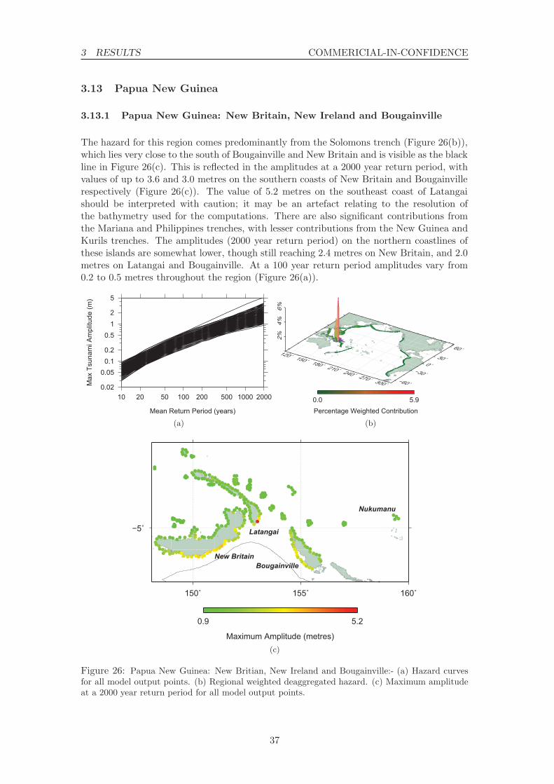
3.13 Papua New Guinea
3.13.1 Papua New Guinea: New Britain, New Ireland and Bougainville
The hazard for this region comes predominantly from the Solomons trench (Figure 26(b)),which lies very close to the south of Bougainville and New Britain and is visible as the blackline in Figure 26(c). This is reflected in the amplitudes at a 2000 year return period, withvalues of up to 3.6 and 3.0 metres on the southern coasts of New Britain and Bougainvillerespectively (Figure 26(c)). The value of 5.2 metres on the southeast coast of Latangaishould be interpreted with caution; it may be an artefact relating to the resolution ofthe bathymetry used for the computations. There are also significant contributions fromthe Mariana and Philippines trenches, with lesser contributions from the New Guinea andKurils trenches. The amplitudes (2000 year return period) on the northern coastlines ofthese islands are somewhat lower, though still reaching 2.4 metres on New Britain, and 2.0metres on Latangai and Bougainville. At a 100 year return period amplitudes vary from0.2 to 0.5 metres throughout the region (Figure 26(a)).
0.02
0.050.10.2
0.512
5
Max
Tsu
nam
i Am
plitu
de (m
)
10 20 50 100 200 500 1000 2000
Mean Return Period (years)
(a)
120˚ 150˚ 180˚ 210˚ 240˚ 270˚ 300˚ −60˚
−30˚0˚
30˚
60˚
2%4%
6%
0.0 5.9Percentage Weighted Contribution
(b)
150˚ 155˚ 160˚
−5˚
0.9 5.2
Maximum Amplitude (metres)
New Britain
Latangai
Bougainville
Nukumanu
(c)
Figure 26: Papua New Guinea: New Britian, New Ireland and Bougainville:- (a) Hazard curvesfor all model output points. (b) Regional weighted deaggregated hazard. (c) Maximum amplitudeat a 2000 year return period for all model output points.
37
3 RESULTS COMMERICIAL-IN-CONFIDENCE
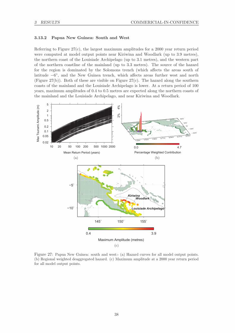
3.13.2 Papua New Guinea: South and West
Referring to Figure 27(c), the largest maximum amplitudes for a 2000 year return periodwere computed at model output points near Kiriwina and Woodlark (up to 3.9 metres),the northern coast of the Louisiade Archipelago (up to 3.1 metres), and the western partof the northern coastline of the mainland (up to 3.3 metres). The source of the hazardfor the region is dominated by the Solomons trench (which affects the areas south oflatitude −6◦, and the New Guinea trench, which affects areas further west and north(Figure 27(b)). Both of these are visible on Figure 27(c). The hazard along the southerncoasts of the mainland and the Louisiade Archipelago is lower. At a return period of 100years, maximum amplitudes of 0.4 to 0.5 metres are expected along the northern coasts ofthe mainland and the Louisiade Archipelago, and near Kiriwina and Woodlark.
0.02
0.050.10.2
0.512
5
Max
Tsu
nam
i Am
plitu
de (m
)
10 20 50 100 200 500 1000 2000
Mean Return Period (years)
(a)
120˚ 150˚ 180˚ 210˚ 240˚ 270˚ 300˚−60˚
−30˚0˚
30˚
60˚2%
4%
0.0 4.7Percentage Weighted Contribution
(b)
145˚ 150˚ 155˚
−10˚
−5˚
0.4 3.9
Maximum Amplitude (metres)
Louisiade Archipelago
KiriwinaWoodlark
(c)
Figure 27: Papua New Guinea: south and west:- (a) Hazard curves for all model output points.(b) Regional weighted deaggregated hazard. (c) Maximum amplitude at a 2000 year return periodfor all model output points.
38

3 RESULTS COMMERICIAL-IN-CONFIDENCE
3.14 Samoa
The southern coastlines of Savaii and Upolu have the highest hazard, with maximumamplitudes at a 2000 year return period of the order of 2.3 to 3.4 metres (Figure 28(c)).This is due to the proximity of the Tonga trench, which lies just to the south and is theonly significant source of hazard for the region (Figure 28(b)). Maximum amplitudes onthe northern coastlines are lower, but still significant, particularly in the case of Upolu (upto 2.0 metres). At a return period of 100 years maximum amplitudes of up to 0.6 metrescan be expected on the southern coasts of Savaii and Upolu.
In Western Samoa the tsunami generated by the 1960 Chile earthquake was alsomost pronounced at Fagaloa Bay (Upolu) where the maximum run-up (the highest pointabove sea level reached by the wave) was estimated to be about 2.5 metres (Keys, 1963).Minor damage to buildings was sustained and it was reported that the waves carried fueldrums 73 metres inland. Residents, who had been forewarned by announcements on thelocal radio station, had taken refuge on higher ground and no loss of life occurred. Therest of Western Samoa appears to have escaped undamaged, probably because of screeningby offshore reefs, which are absent from Fagaloa Bay (Keys, 1963).
0.02
0.050.10.2
0.512
5
Max
Tsu
nam
i Am
plitu
de (m
)
10 20 50 100 200 500 1000 2000
Mean Return Period (years)
(a)
120˚ 150˚ 180˚ 210˚ 240˚ 270˚ 300˚ −60˚−30˚
0˚30˚
60˚
5%10
%15
%
0.0 14.3Percentage Weighted Contribution
(b)
188˚
−14˚
0.7 3.4
Maximum Amplitude (metres)
Savaii
Upolu
(c)
Figure 28: Samoa:- (a) Hazard curves for all model output points. (b) Regional weighted deaggre-gated hazard. (c) Maximum amplitude at a 2000 year return period for all model output points.
39

3 RESULTS COMMERICIAL-IN-CONFIDENCE
3.15 The Solomon Islands
The Solomons and New Hebrides trenches are the only significant sources of hazard forthis region (Figure 29(b)), with the Solomons trench, which is visible on Figure 29(c),dominating. The southern coastlines of Makira, Guadalcanal and New Georgia, and thenorthern shore of Rennell have the highest hazard, with maximum amplitudes of around1.7 to 3.7 metres (Figure 29(c)). At a return period of 100 years maximum amplitudes of0.2 to 0.5 metres can be expected at all model output points in the region (Figure 29(a)).
0.02
0.050.10.2
0.512
5
Max
Tsu
nam
i Am
plitu
de (m
)
10 20 50 100 200 500 1000 2000
Mean Return Period (years)
(a)
120˚ 150˚ 180˚ 210˚ 240˚ 270˚ 300˚−60˚
−30˚0˚30˚
60˚
2%4%
6%
0.0 5.3Percentage Weighted Contribution
(b)
160˚ 165˚
−10˚
−5˚
1.0 3.7
Maximum Amplitude (metres)
Makira
Guadalcanal
Rennell
New Georgia
Santa CruzIslands
Ontong Java
(c)
Figure 29: Solomon Islands:- (a) Hazard curves for all model output points. (b) Regional weighteddeaggregated hazard. (c) Maximum amplitude at a 2000 year return period for all model outputpoints.
40

3 RESULTS COMMERICIAL-IN-CONFIDENCE
3.16 Tokelau
The hazard is relatively uniform over all model output points in Tokelau, with maximumamplitudes for a 2000 year return period ranging from 1.0 to 1.4 metres, and 0.2 to 0.3metres at a return period of 100 years (Figures 30(a) and 30(c)). The most significantsources of hazard are the New Hebrides trench and the northern part of the Tonga trench,with smaller contributions from the Kurils trench and the Peru and Chile trenches (Fig-ure 30(b)).
0.02
0.050.10.2
0.512
5
Max
Tsu
nam
i Am
plitu
de (m
)
10 20 50 100 200 500 1000 2000
Mean Return Period (years)
(a)
120˚ 150˚ 180˚ 210˚ 240˚ 270˚ 300˚ −60˚−30˚
0˚30˚
60˚
1%2%
3%
0.0 2.7Percentage Weighted Contribution
(b)
188˚
−9˚
1.0 1.4
Maximum Amplitude (metres)
Atafu
Nukunonu
Fakaofo
(c)
Figure 30: Tokelau:- (a) Hazard curves for all model output points. (b) Regional weighted deag-gregated hazard. (c) Maximum amplitude at a 2000 year return period for all model output points.
41

3 RESULTS COMMERICIAL-IN-CONFIDENCE
3.17 Tonga
Tonga lies just to the west of the Tonga trench, which is the source of hazard for this nation(Figure 31(b)) and part of which is visible in Figure 31(c). At a return period of 2000years, maximum amplitudes of up to 3.6 metres off Tongatapu, 3.9 metres off Haapai, 4.7metres off Hunga and 4.3 metres off Niuatoputapu can be expected (Figure 31(c)). In themore westerly islands maximum amplitudes are lower but are still potentially hazardous,for example up to 2.1 metres in Niuafoou. At a return period of 100 years, maximumamplitudes of up to 0.7 metres can be expected in the same regions (Figure31(b)).
0.02
0.050.10.2
0.512
5
Max
Tsu
nam
i Am
plitu
de (m
)
10 20 50 100 200 500 1000 2000
Mean Return Period (years)
(a)
120˚ 150˚ 180˚ 210˚ 240˚ 270˚ 300˚ −60˚−30˚
0˚30˚
60˚
2%4%
6%8%
0.0 7.5Percentage Weighted Contribution
(b)
184˚ 186˚
−20˚
−18˚
−16˚
1.6 4.7
Maximum Amplitude (metres)
Tongatapu
Hunga
Niuatoputapu
Niuafoou
Haapai
(c)
Figure 31: Tonga:- (a) Hazard curves for all model output points. (b) Regional weighted deaggre-gated hazard. (c) Maximum amplitude at a 2000 year return period for all model output points.
42
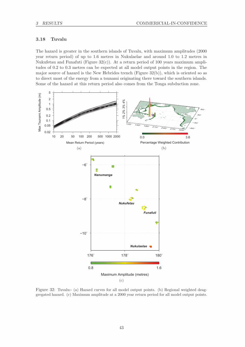
3 RESULTS COMMERICIAL-IN-CONFIDENCE
3.18 Tuvalu
The hazard is greater in the southern islands of Tuvalu, with maximum amplitudes (2000year return period) of up to 1.6 metres in Nukulaelae and around 1.0 to 1.2 metres inNukufetau and Funafuti (Figure 32(c)). At a return period of 100 years maximum ampli-tudes of 0.2 to 0.3 metres can be expected at all model output points in the region. Themajor source of hazard is the New Hebrides trench (Figure 32(b)), which is oriented so asto direct most of the energy from a tsunami originating there toward the southern islands.Some of the hazard at this return period also comes from the Tonga subduction zone.
0.02
0.050.10.2
0.512
5
Max
Tsu
nam
i Am
plitu
de (m
)
10 20 50 100 200 500 1000 2000
Mean Return Period (years)
(a)
120˚ 150˚ 180˚ 210˚ 240˚ 270˚ 300˚−60˚
−30˚
0˚
30˚
60˚
1%2%
3%4%
0.0 3.6Percentage Weighted Contribution
(b)
176˚ 178˚ 180˚
−10˚
−8˚
−6˚
0.8 1.6
Maximum Amplitude (metres)
Nukulaelae
Funafuti
Nukufetau
Nanumanga
(c)
Figure 32: Tuvalu:- (a) Hazard curves for all model output points. (b) Regional weighted deag-gregated hazard. (c) Maximum amplitude at a 2000 year return period for all model output points.
43

3 RESULTS COMMERICIAL-IN-CONFIDENCE
3.19 Vanuatu
The New Hebrides trench, visible on Figure 33(c), lies just to the west of Vanuatu andis the primary source of hazard for the region (Figure 33(b)). Maximum amplitudes fora 2000 year return period are significantly higher at model output points on the westernshores of the major islands over those on the eastern shores, with values of over 4.0 me-tres on Espiritu Santo, Malakula, Efate, Erromango, Tanna and Aneityum (Figure 33(c)).Maximum amplitudes at the more easterly islands are lower, though still potentially haz-ardous; for example they reach 1.9 metres near Pentecost. At a 100 year return periodmaximum amplitudes of up to 0.6 to 0.7 metres can be expected at some model outputpoints.
0.02
0.050.10.2
0.512
5
Max
Tsu
nam
i Am
plitu
de (m
)
10 20 50 100 200 500 1000 2000
Mean Return Period (years)
(a)
120˚ 150˚ 180˚ 210˚ 240˚ 270˚ 300˚−60˚
−30˚0˚
30˚60˚
2%4%
6%
0.0 5.5Percentage Weighted Contribution
(b)
168˚ 170˚
−20˚
−18˚
−16˚
−14˚
1.1 4.7
Maximum Amplitude (metres)
Efate
Malakula
Erromango
Tanna
Aneityum
Maewo
Pentecost
Espiritu Santo
(c)
Figure 33: Vanuatu:- (a) Hazard curves for all model output points. (b) Regional weighteddeaggregated hazard. (c) Maximum amplitude at a 2000 year return period for all model outputpoints.
44

4 CONCLUSION COMMERICIAL-IN-CONFIDENCE
4 Conclusion
In summary, by segmenting the Pacific Rim subduction zones we have modelled nearly60,000 tsunami to offshore of all the SOPAC nations. The probability of each tsunami wasestimated by determining what fraction of the global seismicity would be expected on eachzone and partitioning the global seismicity accordingly. For each subduction zone a rangeof different maximum magnitudes and earthquake source geometry models were includedin the final hazard assessment presented here.
This assessment was designed to allow SOPAC to prioritise which nations have thehighest tsunami hazard and should be considered for future, more detailed, study. Thenations with the highest hazard at the 1 in 2000 year return period level are listed inTable 1 and the hazard curves for the point with the highest hazard in each nation areshown in Figure 34.
Several major conclusions can be drawn from the report:
• Several nations have a very high tsunami hazard. These nations are usually closeto a major subduction zone and are perpendicular to it (eg PNG, New Caledonia,Tonga, Guam, Vanuatu). The nearest zone dominates the hazard for these nations,particularly at longer return periods. If a large earthquake occurred at a zone veryclose to the country, the tsunami may arrive before any warning from any of theglobal warning centres.
• The SOPAC nations located near the centre of the Pacific have a more moderatehazard, but the sources of the hazard are spread out over a larger number of zonesaround the Pacific Rim. Potentially dangerous tsunami for these islands can comefrom a large number of different directions towards the islands.
For more details on specific nations, please see the relevant section in Section 3, the kmlfiles on the accompaning DVD or contact Geoscience Australia directly.
While we believe the overall results of this study are reliable and are useful, we dorecommend that more detailed studies be undertaken, particularly of the nations with thehighest hazard. In particular, future studies should use a higher resolution and more accu-rate bathymetry for the southwest Pacific islands. The resolution of the bathymetry usedhere is not high enough to determine precisely the offshore heights with great confidence,given the complex bathymetry of the region. However, we believe the relative levels ofhazard are reliable.
The other major source of uncertainity in this assessment is with our estimate of theliklihood of a major (Mw8+) event for many of the zones. In this assessment, we estimatedthis liklihood by extrapolating from the frequency of smaller earthquakes. However, wecannot be sure that any given zone can, or ever has, produced an earthquake larger thanhas been observed for the zone. The only way to reduce this uncertainity is by studiesinto the palaeo-record of specific islands for evidence of pre-historic large inundations fromtsunami. However, given the scale of the problem this is likely to be a slow task.
It is also important to note that high offshore wave heights do not always correspondto high onshore run-ups or large amounts of damage. If the bulk of a island’s populationis close to sea level then even a moderate to low tsunami may have the potential to causesignificant damage. Therefore we recommend more detailed inundation studies of the
45

4 CONCLUSION COMMERICIAL-IN-CONFIDENCE
French Polynesia
PalauSamoa
F. S. of Micronesia
Vanuatu
Tokelau
Marshall Islands
Papua New Guinea
Cook Islands
Kiribati
Tonga
Nauru
Guam
Solomon Islands
Niue
Tuvalu
Fiji
American Samoa
New Caledonia
0.05
0.1
0.2
0.5
1
2
5
Max
Tsu
nam
i Am
plitu
de (m
etre
s)
10 20 50 100 200 500 1000 2000
Mean Return Period (years)
Figure 34: Hazard curves for the nations in the study. For each return period the curve gives themaximum value of the amplitude taken over all the model output points of that nation.
potentially at risk communties be undertaken in order to more confidently quantify thepotential impact to the SOPAC nations of a major tsunami reaching the islands.
46
4 CONCLUSION COMMERICIAL-IN-CONFIDENCE
References
Allport, J.K. and R.J. Blong, 1995. The Australian Tsunami Database (ATDB),Sydney: School of Earth Sciences, Macquarie University.
Barrientos, S.E. and S.N. Ward, 1990. The 1960 Chile earthquake: inversion for slipdistribution from surface deformation. Geophys. J. Int. 103, pp.589-598.
Bryant, E., 2001. Tsunami: the underrated hazard, Cambridge University Press,Cambridge.
Bassin, C., Laske, G. and G. Masters, 2000. The current limits of resolution forsurface wave tomography in North America, EOS Trans AGU, 81, F897.http://mahi.ucsd.edu/Gabi/rem.html.
Bathgate, J., Volti T.. and Greenslade, D. J. M., 2008. The Joint Australian TsunamiWarning Centre: responding to a tsunamigenic earthquake - Puysegur Trench,30 September 2007. Preview, 133, April 2008, pp. 40-44.
Bird, P., 2003. An updated digital model of plate boundaries. Geochem. Geophys.Geosys. 4(3), 1027, doi:10.1029/2001GC000252.
Burbidge, D., Cummins, P. and Mleczko R., 2007. A Probablistic Tsunami HazardAssessment for Western Australia: Report to the Fire and Emergency ServicesAuthority of Western Australia, Geoscience Australia.
Burbidge, D., Mleczko, R., Thomas, C., Cummins, P., Nielsen, O. and T. Dhu,2008. A Probabilistic Tsunami Hazard Assessment for Australia. GeoscienceAustralia Professional Opinion. No.2008/04.
Gudmundsson , O. and M. Sambridge, 1998. A regionalized upper mantle (RUM)seismic model, J. Geophys. Res. B4, pp.7121-7136.
ICMMG - see Institute of Computational Mathematics and Mathematical Geophysics.
Johnson, R. W., 1987. Large-scale volcanic cone collapse: the 1888 slope failure ofRitter volcano, and other examples from Papua New Guinea. Bull. Volcanol.49, pp.669-679.
Keys, J.G., 1963. The tsunami of 22 May 1960 in the Samoa and Cook Islands. Bull.Seism. Soc. Am. 53(6), pp.1211-1227.
Kopp, H. and N. Kukowski, 2003. Backstop geometry and accretionary mechanics ofthe Sunda margin, Tectonics, 22, 6, 1072, doi:10.1029/2002TC001420.
Mader, C.L., 2002. Modeling the 1958 Lituya Bay mega-tsunami, II. Sci. of Tsun.Haz. 20(5), pp.241-250.
Mei, C., Stiassnie, M. and D. Yue, 2005. Theory and Applications of Ocean SurfaceWaves. Singapore: World Scientific.
Myles, D., 1986. The Great Waves. London: Robert Hale.
Narayan, J. P., Sharma, M. L. and B.K. Maheshwari, 2005. Effects of Medu andcoastal topography on the damage pattern during the recent Indian Oceantsunami along the coast of Tamilnadu. Sci. Tsunami Haz. 23(2), pp.9-18.
National Geophysical Data Centre, 2007. Global Tsunami Database, National Oceanicand Atmospheric Administration, Washington, viewed 23 May 2007,<http://ngdc.noaa.gov/seg/hazard/tsu db.shtml>.
NGDC - see National Geophysical Data Centre.
47
4 CONCLUSION COMMERICIAL-IN-CONFIDENCE
Okal, E.A., Borrero, J. and C.E. Synolakis, 2004. The earthquake and tsunami of1865 November 17: evidence for far-field tsunami hazard from Tonga. Geophys.J. Int. 157, pp.154-174.
Song, Y.T., Ji, C., Fu, L.-L., Zlotnicki, V., Shum, C.K., Yi, Y. and V. Hjorleifs-dottir, 2005. The 26 December 2004 tsunami source estimated from satel-lite radar altimetry and seismic waves. Geophys. Res. Lett. 32, L20601,doi:10.1029/2005GL023683.
Taylor, F.W., Edwards, R.L., Wasserburg, G.J. and C. Frohlich, 1990. Seismic recur-rence intervals and timing of aseismic subduction inferred from emerged coralsand reefs of the Central Vanuatu (New Hebrides) Frontal Arc. J. Geophys.Res. 95(B1), pp.393-408.
Thomas, C., Burbidge, D., and P. Cummins, 2007. A Preliminary Study into theTsunami Risk faced by Southwest Pacific Nations, Geoscience Australia.
Wang, R., Martin, F.L., and F. Roth, 2006. Computation of deformation induced byearthquakes in a multi-layered crust – FORTRAN programs EDGRN EDCMP.Comp. and Geosc. 29, pp.195-207 (inc. erratum).
Webster, M. A. and P. Petkovic, 2005. Australian Bathymetry and Topography Grid,June 2005, Geoscience Australia, Record 2005/12.
Wells, D. L. and K. J. Coppersmith, 1994. New empirical relationships among mag-nitude, rupture length, rupture width, rupture area and surface displacement,BSSA, 84(4), 974-1002.
Wessel, P. and W. H. F. Smith, 1991. Free software helps map and display data,EOS Trans, AGU, 72, 441.
48

A PTHA METHOD COMMERICIAL-IN-CONFIDENCE
Appendix A PTHA Method
A.1 Summary
The probabilistic tsunami hazard assessment undertaken in this study seeks to assess theprobabilities of certain waveheights being exceeded due to the arrival of a tsunami at thelocations under investigation. These probabilities are expressed in terms of expected returnperiods. This method has been used previously (for example in Burbidge et al, 2007, 2008)and is based on a well established method of probabilistic seismic hazard assessments.Broadly, it involves producing and analysing a very large catalogue of synthetic tsunamiwhich is produced by combining, in various ways, a much smaller number of synthetictsunami. The steps involved are:
1. Determine the locations at which the assessment of hazard will be made (the modeloutput points, see Figure 2).
2. Create a model of the faults to be considered (that is, the location and geometry ofthe subduction zones under consideration, Figure 5).
3. Segment these faults into smaller fixed size subfaults. In this study, subfaults con-sisting of 100 × 50 kilometre rectangular segments were used (Figure 36).
4. Model the deformation of the sea floor produced by an earthquake involving onemetre of slip on each subfault, and model the propagation of the resulting tsunamito each of the model output points.
5. Create a catalogue of synthetic earthquakes along the faults, containing values fortheir location, area, magnitude, and the probability that each event might occur.
6. Determine which subfaults fall within the rupture area of each synthetic earthquake,and to what extent each such subfault contributes to the synthetic event (that is,what slip should be attributed to the subfault).
7. Combine the modelled tsunami produced by each contributing subfault (from Step 4)to estimate the tsunami produced by the synthetic event.
8. Aggregate over the resulting catalogue of synthetic tsunami to determine relationshipsbetween maximum tsunami amplitudes and their probabilities.
In this study the tsunami from a total of 983 subfaults were combined in different ways toproduce a catalogue of 59,871 synthetic tsunami.
More detailed information on the method used is presented below.
A.2 Bathymetry
The bathymetry was based on a combination of the US Naval Research Laboratory’s twominute Digital Bathymetric Database (DBDB2) and Geoscience Australia’s 250 metredataset (Webster & Petkovic, 2005), which was resampled to a regular grid of locationsspaced two arc minutes apart. This is a ‘generic’ bathymetry dataset and, while there arehigher resolution data available for some parts of the study region, because of the very largestudy area it was not possible to perform the computations at a higher resolution with the
49

A PTHA METHOD COMMERICIAL-IN-CONFIDENCE
computational resources available. Two arc minutes (≈ 3.7 kilometres) is considered to bean adequate resolution for modelling the propagation of tsunami in the open ocean in deepwater, and since the model output points were chosen to lie in water at least 100 metresdeep (see Section A.3), for the most part the resolution will be adequate for modelling thetsunami amplitudes at those points. However there are several effects of the resolutionthat should be noted:
• In many nations the bathymetry is very steep so that neighbouring bathymetric gridpoints may fall on dry land and in water as deep as several thousand metres.
• Some very small islands may not be represented in the bathymetry at all, that is,there may be no ‘dry’ grid point that represents the island (see Figure 35). In sucha case the semi-automatic procedure adopted for selection of model output points(Section A.3) may not place a model output point near that island, and consequentlythere may be some very small inhabited islands within the nations included in thisstudy that are not represented by model output points.
• Regions of very complex and rapidly varying bathymetry may not be adequatelyrepresented by the bathymetric dataset, and in these regions the modelling of thetsunami amplitudes must be interpreted with caution. One such region is the ChuukIslands, in the Federated States of Micronesia, shown in Figure 35. While the majorislands are represented, it is unlikely that the resolution of the bathymetry in thisregion is sufficient to allow adequate modelling of tsunami amplitudes at points closeto these islands.
152˚
7˚30'
dry wet
Figure 35: The Chuuk Islands in the Federated States of Micronesia. The background is thebathymetric grid used in the study, categorised into wet or dry areas. The grid lines indicatethe resolution (two arc minutes) of the grid. The coastlines are overlaid using the full resolutioncoastline dataset available as part of the Generic Mapping Tools (GMT see Wessel & Smith (1991)).
50

A PTHA METHOD COMMERICIAL-IN-CONFIDENCE
A.3 Model Output Points
The model output points were produced by determining the bathymetric grid points thatare as close as possible to each of the SOPAC nations, but at least 100 metres deep. Theresulting set of grid points was thinned to reduce data volume, and edited manually toensure that populated islands (according to the LandScanTM 2004 dataset) were adequatelyrepresented. The locations of the 2875 model output points used in the study are shownin Figure 2. While the water depth at each model output point is at least 100 metres,in many cases it may be much deeper, because of the steeply varying bathymetry in theregion of some of the nations in the study, and the resolution of the bathymetry data used.In order to be able to compare results from output points at different depths, Green’s Law(see for example Mei et al, 2005) has been used to normalise all results to a nominal depthof 100 metres. Thus if zactual is the modelled waveheight at an output point of depth d,then the normalised waveheight at that output point,
z = zactual
(d
100
) 14
may be considered to be the equivalent waveheight at a depth of 100 metres if there is nofocussing or de-focussing of the wave between the two points. All results in this study wereexpressed in terms of these normalised waveheights.
A.4 Fault Model
This was based on the plate model of Bird (2003). The dip was estimated from the RegionalUpper Mantle (RUM) model of Gudmundsson and Sambridge (1998) or from papers basedon seismic surveys of specific subduction zones. A map of the 983 subfaults used in thisassessment is shown in Figure 36. The subfaults in this figure are coloured according todepth.
A.5 Numerical Modelling of Sea Floor Deformation and Tsunami Prop-agation
The sea floor deformation was calculated by representing the fault as a dislocation in alayered elastic media. The elastic properties of the crust were based on CRUST2.0 (Bassinet al, 2000) and Kopp and Kukowski (2003). The general method used to calculate the seafloor deformation is described in more detail in Wang et al (2006).
The tsunami propagation was modelled using a staggered grid finite difference schemeto numerically solve the linear shallow water wave equations.
A.6 Catalogue of Synthetic Earthquakes
The earthquake catalogue was developed using a logic tree approach. Each branch ofthe tree represents some characteristic of an earthquake, for example magnitude, area ordepth, and has an associated probability. The tips of the outermost branches representthe synthetic earthquakes, and the probability of each earthquake is the product of theprobabilities of those branches of the tree leading to that earthquake.
51

A PTHA METHOD COMMERICIAL-IN-CONFIDENCE
120˚ 140˚ 160˚ 180˚ 200˚ 220˚ 240˚ 260˚ 280˚ 300˚
−60˚
−40˚
−20˚
0˚
20˚
40˚
60˚
0 10 20 30 40 50 60
metres
Figure 36: Location of the 983 subfaults used in the study, showing the depth of thecentroid of each subfault.
Activity rates were based on the fault slip derived from plate motion rates and thelength and geometry of each subduction zone. The method used is similar to the onedescribed in Burbidge et al (2008) except that the variable dip of the faults was takeninto consideration. The recurrence was assumed to obey the Gutenburg-Richter relationup until a maximum magnitude cut-off value that differed for each zone. For most zonesfour different cut-off values were used. Every magnitude between 7.0 and the maximumwas modelled at increments of 0.1 magnitude units. For most modelled magnitudes, twodifferent possible rupture areas and two different possible rupture lengths were includedin the catalogue. The Wells and Coppersmith (1994) relations were used to determine thearea and length as a function of magnitude. In total, 59,871 earthquakes were included inthis assessment.
A.7 Deaggregating the Hazard
Deaggregation of the hazard allows the source of the hazard at a particular location tobe identified, or over a region as a whole. There are a number of ways of deaggregatinghazard and this section is devoted to an explanation of the methods adopted in this study.
A.7.1 Deaggregated Hazard Maps
A deaggregated hazard map allows the main sources of the hazard to be identified for asingle offshore location for a single return period:
52

A PTHA METHOD COMMERICIAL-IN-CONFIDENCE
1. Choose the return period and the offshore location (model output point) at whichthe deaggregation is to be performed.
2. Determine the maximum expected tsunami amplitude at the chosen model outputpoint for the chosen return period.
3. Find all events in the synthetic catalogue of tsunami that produce a wave that exceedsthis amplitude at the given model output (call these the exceedance events), alongwith their probabilities.
4. For each exceedance event, find the subfaults that constitute that event and apportionthe probability of the event equally among those subfaults.
5. Sum these probabilities over all the exceedance events, to calculate a probability foreach of the 982 subfaults.
6. Express the results as a percentage contribution from each subfault.
7. Map these contributions.
A.8 Regional Weighted Deaggregated Hazard Maps
Each deaggregated hazard map is peculiar to the model output point for which it is pro-duced, and indicates the source of the hazard at that particular model output point only.Thus it is possible for a deaggregated hazard map for a point on one side of an island toindicate that the main source of the hazard at that point is the Chile trench, for example,while such a map for a point on the other side of the island might indicate that the majorsource of hazard for that point is the Tonga trench. A regional weighted deaggregatedhazard map gives some indication of the source of hazard to the region as a whole:
1. Choose the return period.
2. Deaggregate the hazard as described above for all the model output points, to obtainthe relative contributions of each of the subfaults, for every model output point.
3. Weight the contributions of each subfault at each model output point by the maxi-mum tsunami amplitude for the chosen return period at that model output point.
4. Sum the results over all the model output points, and express as a percentage of thetotal contribution.
53

B VALIDATION: KURIL ISLANDS, 15/11/2006 COMMERICIAL-IN-CONFIDENCE
Appendix B Validation: Kuril Islands, 15/11/2006
On 15 November 2006 a magnitude 8.3 earthquake occurred at 153.230◦E 46.607◦N off theKuril Islands (Figure 37) which produced a tsunami across the Pacific with measured waveheights of (for example) 88 cm at Hawaii, 176 cm at Crescent City, California, and 57 cmat Samoa (according to the USGS). The modelling procedures used in this study have beenvalidated against a detailed finite fault model for this earthquake published by the USGS,and data from ocean bottom pressure gauges deployed by the US Government’s NationalOceanic and Atmospheric Administration (DART gauges) and by the Japanese Agencyfor Marine-Earth Science and Technology (JAMSTEC). The locations of these gauges areshown in Figure 37.
Figure 37: Numerical model of the Kuril Islands earthquake and tsunami of 15 November2006, with the locations of the DART (circles) and JAMSTEC (triangles) ocean bottompressure gauges.
Using the techniques discussed in Appendix A, the finite fault model published byUSGS was used to compute an estimate of the sea floor deformation due to the KurilIslands event and the propagation of the resulting tsunami was modelled. Results of thenumerical simulations were calculated at the location of the ocean bottom pressure gaugesfor comparison with the actual water levels recorded by the gauges. It was necessaryto filter the pressure gauge data to remove extraneous signals, primarily ocean tides andhigh frequency components that are not part of tsunami waveforms. The comparisonsare presented on the following pages, with the filtered pressure gauge signals in blue andthe model results in red. Overall the model results agree well with the pressure gaugedata, particularly for the first peak and trough of the waveform. While there are somedifferences in phase, the amplitudes and arrival times are in good agreement. On averagethe maximum amplitudes agree to within 23%. As well as possible shortcomings in themodelling procedure (including limitations in the bathymetric model used), such differencesas there are can be attributed to a disparity between the actual earthquake rupture andthe USGS finite fault model, and the filtering process used for removing tidal componentsfrom the observed pressure data.
54

B VALIDATION: KURIL ISLANDS, 15/11/2006 COMMERICIAL-IN-CONFIDENCE
Figure 38: (a – f) Comparison of ocean pressure gauge data (blue) and model results (red)for the Kuril earthquake and tsunami of 15 November 2006.
55
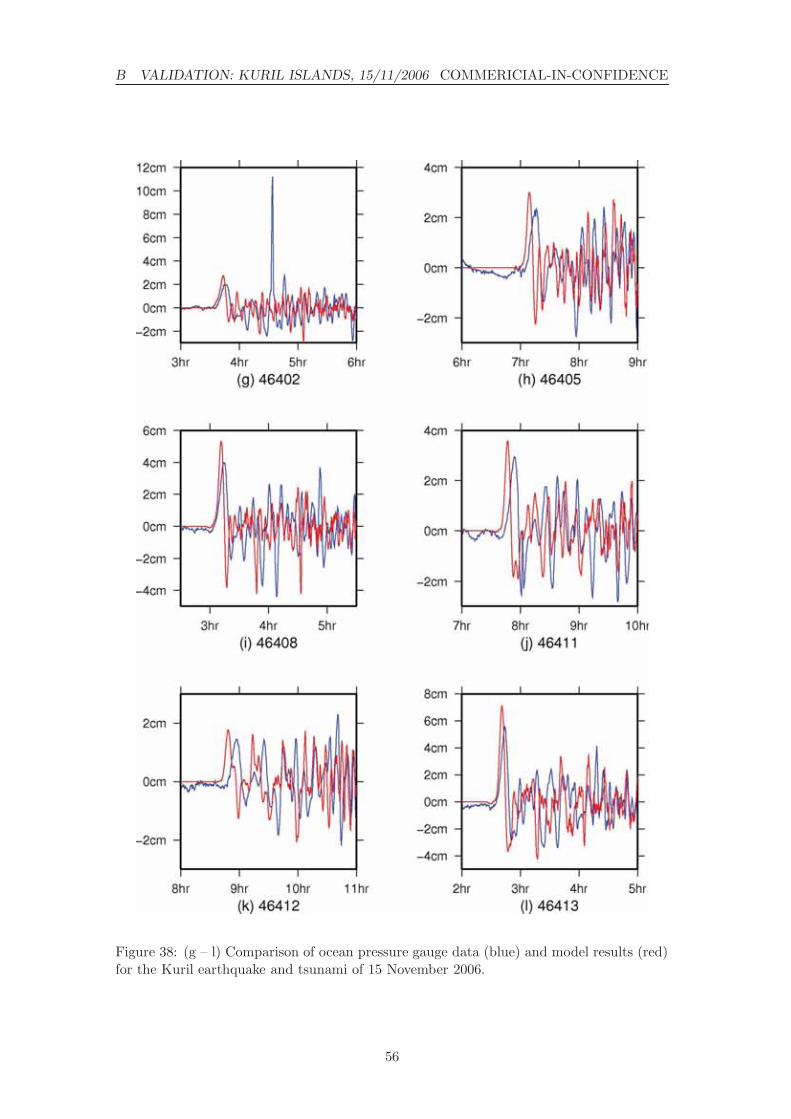
B VALIDATION: KURIL ISLANDS, 15/11/2006 COMMERICIAL-IN-CONFIDENCE
Figure 38: (g – l) Comparison of ocean pressure gauge data (blue) and model results (red)for the Kuril earthquake and tsunami of 15 November 2006.
56

B VALIDATION: KURIL ISLANDS, 15/11/2006 COMMERICIAL-IN-CONFIDENCE
Figure 38: (m) Comparison of ocean pressure gauge data (blue) and model results (red)for the Kuril earthquake and tsunami of 15 November 2006.
The spike in the signal from DART buoy 46402 is likely to be a data error and is webelieve is probably not part of the tsunami signal.
The DART and JAMSTEC buoys are in water several thousand metres deep. It hasnot been possible to validate the modelling procedure against data from shallower waterbecause such data come from instruments such as harbour tide gauges that typically arein water only a few metres deep, where the model is not valid. There is some concern thatthe bathymetric grid resolution employed may not be high enough to always adequatelyrepresent the waveforms, particularly in shallower water where their wavelength will beshorter.
57

C VALIDATION: CHILE, 22/05/1960 COMMERICIAL-IN-CONFIDENCE
Appendix C Validation: Chile, 22/05/1960
On 22 May 1960 the largest earthquake ever recorded with modern seismographs (Mw 9.5)occurred off the coast of Chile (at approximately 286.5◦E, 41◦S). This produced a Pacificwide tsunami that caused widespread damage, particularly along the coasts of Chile, Hawaiiand Japan.
The techniques of Appendix A have been used to estimate the sea floor deformationproduced by this event and to model the resulting tsunami, based on a uniform slip modelfor the earthquake presented by Barrientos and Ward (1990). Figure 39 shows the resultsof this modelling.
In Western Samoa the tsunami was most pronounced at Fagaloa Bay (Upolu) wherethe maximum run-up (the highest point above sea level reached by the wave) was estimatedto be about 2.5 metres (Keys, 1963). Minor damage to buildings was sustained and itwas reported that the waves carried fuel drums 73 metres inland. Residents, who hadbeen forewarned by announcements on the local radio station, had taken refuge on higherground and no loss of life occurred. The rest of Western Samoa appears to have escapedundamaged, probably because of screening by offshore reefs, which are absent from FagaloaBay (Keys, 1963). In American Samoa the tsunami reached a maximum run-up height ofover three metres at Pago Pago village (Allport and Blong, 1995). Buildings were movedoff their foundations and a house washed into the bay. No loss of life was reported.
In Fiji reports appear to be confined to the effects in Suva harbour. The maximumrunup was reported to be about 0.5 metres, and the tsunami induced a powerful surge inthe harbour. Many boats sustained damage, but no loss of life was recorded (Allport andBlong, 1995).
In French Polynesia many of the islands are protected by outer reefs and deep lagoons,with rather steep bathymetry offshore, and in most cases only slight damage was sustained.No loss of life was recorded. The average runup surveyed in Tahiti was 1.7 metres. Largerrunups, up to 3.4 metres, were recorded along the north shore of the island which is moreexposed to the open ocean (Vitousek, 1963). The greatest effects in French Polynesiawere felt in the Marquesas Islands which have few outer reefs and more gradual changesin offshore bathymetry. Runups of at least 4.5 metres (possibly up to nine metres) wereobserved. Destruction of buildings near the shore was reported (Vitousek, 1963).
The Hawaiian islands suffered extensive damage and 61 deaths. The island of Hawaiibore the brunt of the damage, mostly around Hilo where all the deaths and most of thedamage occurred. Damage to buildings was extensive in this area, with almost totaldestruction in an area of nearly 300 acres. Rocks weighing up to 22 tonnes were carried180 metres inland. There was considerable damage to houses and commercial buildings onMaui, with some being destroyed. The other islands suffered only minor damage (Cox andMink, 1963).
In Japan, run-ups of up to 6.4 metres were recorded (ICMMG, 2006), causingwidespread flooding and damage. About 5000 homes were lost leaving 50,000 people home-less, and between 180 and 190 lives were lost (Myles, 1986).
The effects of the tsunami were felt in Australia, with boats removed from theirmoorings in Sydney, Brisbane, Newcastle and Evans Head. Minor damage and floodingwas reported in New Zealand and Papua New Guinea (Allport and Blong, 1995).
In Chile, of course, damage and loss of life were extensive. A maximum run-up of
58

C VALIDATION: CHILE, 22/05/1960 COMMERICIAL-IN-CONFIDENCE
Figure 39: Normalised modelled maximum wave heights of the 1960 Chilean tsunamibased on uniform slip model given by Barrientos and Ward (1990). Wave heights havebeen normalised to 50 metres depth and the maximum is taken over the full time periodof the simulation.
59
C VALIDATION: CHILE, 22/05/1960 COMMERICIAL-IN-CONFIDENCE
25 metres was recorded (NGDC, 2007) and thousands of people drowned. Towns werecompletely obliterated and debris was carried more than three kilometres inland (Myles,1986).
These historical accounts should be read in conjunction with Figure 39. Little damageand no loss of life was reported for coastlines where the incident waves had an offshoreamplitude less than 0.75m (for example Australia, Papua New Guinea and, for the mostpart, New Zealand). However the magnitude of the effect of the tsunami was criticallydependent on local features of the coastline, the height of the tide when the tsunamiarrived and the density of the population in vulnerable areas. This is demonstrated bythe observation that Fiji, Samoa and parts of French Polynesia received with maximumamplitudes between 0.75m and 2.5m but sustained only minor damage, whereas similaramplitude waves offsgire in Hawaii and Japan caused extensive damage and loss of life.Tsunami with offshore amplitude above 2.5m, such as those received along the coast ofChile, resulted in extensive damage and loss of life in South America but not as much inFrench Polynesia.
60