prof. younghee lee 1 1 computer networks u lecture 5: ip addressing-route lookup younghee lee
TRANSCRIPT

1Prof. Younghee Lee1
Computer Networks Lecture 5: IP Addressing-route lookup
Younghee Lee

2Prof. Younghee Lee2
The Internet Protocol Identifier: A sequence number to identify a datagram uniquely. Flag: More bit(indicates the last fragment in original datagram), Don’t Fragment bit(can be
discarded at some subnet->source routing advisable) Fragment offset:: indicate where in the original datagram this fragment belongs Time to live: somewhat similar to a hop count Protocol: the next higher-level protocol

3Prof. Younghee Lee3
Type of Service
TOS subfield: guidance to the IP entity indicating the type or quality of service – The way in which a router learns which routes support whi
ch TOS» Domain administrator preconfigure the TOS associated with the ro
utes» A routing protocol monitor the TOS along the routes monitoring del
ays, throughputs, and dropped datagrams.(ex: OSPF)
Typically ignored now Replaced by DiffServ
4Prof. Younghee Lee4
IPv4 Options
Security: – Security label to be attached to a datagram
Source routing– A sequenced list of router addresses that specifies the routes to be followed.
May be strict or loose Route recording
– allocated to record the sequence of routers visited by the datagram Timestamping
– The source IP entity and some intermediate routers add a time stamp (precision to milliseconds)

5Prof. Younghee Lee5
Naming and Addressing Naming versus addressing
– naming is typically a high-level description– addresses refer to specific physical resources– distinction hard to define but often clear:
» icu.ac.kr» 128.9.23.93» D74A049C2384
Naming/addressing formats– structure: flat versus partitioned (hierarchical)– duration: dynamic versus static– scope: local versus global
Domain Name System (DNS) names are names of hosts DNS binds host names to interfaces Routing binds interface names to paths

6Prof. Younghee Lee6
Name/Address Structure
Hierarchical address space– address space has structure: sequence of fields
» fields identify autonomous organizations, geographical location, ..
– hierarchical can simplifies routing– easily supports distributed assignment of addresses– can result in inefficient use of the address space– example: IP addresses, postal address, telephone
numbers, .. Flat address space
– address has no structure: single field– easier to use full address space– lacks support for routing– example: IEEE addresses (48 bits)

7Prof. Younghee Lee7
IP Addressing: introduction
IP address: 32-bit identifier for host, router interface
interface: connection between host, router and physical link– router’s typically have
multiple interfaces– host may have multiple
interfaces– IP addresses
associated with interface, not host, router
223.1.1.1
223.1.1.2
223.1.1.3
223.1.1.4 223.1.2.9
223.1.2.2
223.1.2.1
223.1.3.2223.1.3.1
223.1.3.27
223.1.1.1 = 11011111 00000001 00000001 00000001
223 1 11
8Prof. Younghee Lee8
IP addresses: how to get one?
Hosts (host portion): hard-coded by system admin in a file DHCP: Dynamic Host Configuration Protocol: dynamically get address: “plu
g-and-play”– host broadcasts “DHCP discover” msg– DHCP server responds with “DHCP offer” msg– host requests IP address: “DHCP request” msg– DHCP server sends address: “DHCP ack” msg
Auto-configuration– IPv6 stateless autoconfiguration– MANET AUTOCONF :
» Standalone» With gateway: can be relatively simple but how to select gateway?» Stand-alone for most of the time but temporarily connected to the infrastructured network
e.g. car network connected while parked and disconnected otherwise» Strong DAD, Prophet, AROD

9Prof. Younghee Lee9
Hierarchical addressing: route aggregation
“Send me anythingwith addresses beginning 200.23.16.0/20”
200.23.16.0/23
200.23.18.0/23
200.23.30.0/23
Fly-By-Night-ISP
Organization 0
Organization 7Internet
Organization 1
ISPs-R-Us“Send me anythingwith addresses beginning 199.31.0.0/16”
200.23.20.0/23Organization 2
...
...
Hierarchical addressing allows efficient advertisement of routing information:
10Prof. Younghee Lee10
IP addressing: the last word...
Q: How does an ISP get block of addresses?
A: ICANN: Internet Corporation for Assigned
Names and Numbers– allocates addresses– manages DNS– assigns domain names, resolves disputes
11Prof. Younghee Lee11
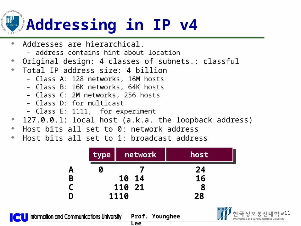
Addressing in IP v4 Addresses are hierarchical.
– address contains hint about location Original design: 4 classes of subnets.: classful Total IP address size: 4 billion
– Class A: 128 networks, 16M hosts– Class B: 16K networks, 64K hosts– Class C: 2M networks, 256 hosts– Class D: for multicast– Class E: 1111, for experiment
127.0.0.1: local host (a.k.a. the loopback address) Host bits all set to 0: network address Host bits all set to 1: broadcast address
typetype networknetwork hosthost
A 0 7 24B 10 14 16C 110 21 8D 1110 28

12Prof. Younghee Lee12
Subnetting
Hierarchy can be extended to more than two layers.
Makes it possible to break up a network in multiple subnets.– provides flexibility to manage
networks– packet forwarding between
subnets is also done using routers, I.e. same as in Internet
Provides autonomy.– subnets inside network are not
visible outside the network
1 0
Network Host
Network HostSubNet
Subnet 1Subnet 3
Subnet 2

13Prof. Younghee Lee13
IP Addressing: Issues
Running out of IP address space: short term solutions.– Classless inter-domain routing– Dynamic address assignment– Network address translation
Longer term solution for IP address shortage: IPv6.– Move to longer addresses: IPv6

14Prof. Younghee Lee14
IP Address Utilization (‘98)
http://www.caida.org/outreach/resources/learn/ipv4space/

15Prof. Younghee Lee15
Problems with Simple Address Structure Address space is not used very efficiently.
– Address spaces for networks can only be 2**8, 2**16, 2**24 in size» Sizes differ by two orders of magnitude
– Organizations that do not fit in smaller network (e.g. 257 hosts) need to use a size that is significantly larger
Running out of addresses.– Especially true for mid-sized networks– Class B – greatest problem
» Sparsely populated – but people refuse to give it back
– Class C too small for most domains– Very few class A – IANA (Internet Assigned Numbers Authority) very
careful about giving
Routing tables are becoming too big.– 100 of thousands of entries
16Prof. Younghee Lee16
Ideas Behind Classless Inter-Domain Routing
Use address space more efficiently by relaxing the strict address structure.– length of network address is variable– generalization of subnetting idea– makes network use more efficient
Have Internet service providers hand out blocks of addresses to their customers.– customers of ISPs appear like subnets of the ISP to other
ISPs– reduces size of the routing tables

17Prof. Younghee Lee17
CIDR Addressing
Length of network address is variable and specified using a netmask.– Can make the address space ju
st large enough
Can merge a group of adjacent class C addresses to form a larger network address.
Network Hosts0
Network Hosts1
1 0
Network Hosts
1 0

18Prof. Younghee Lee18
CIDR Address Allocation: Example
ISP: 128.5.X.X
Customer 1: 128.5.010xxxxx.XCustomer 2: 128.5.110xxxxx.XCustomer 3: 128.5.011xxxxx.X
ISP 4ISP 4
ISPISP
Customer1
Customer1
HostHost
Customer2
Customer2
HostHost
Customer3
Customer3
HostHost
ISP 5ISP 5ISP 3ISP 3
ISP 2ISP 2 HostHostHostHost
HostHost
Single route entry: 128.5/16
19Prof. Younghee Lee19
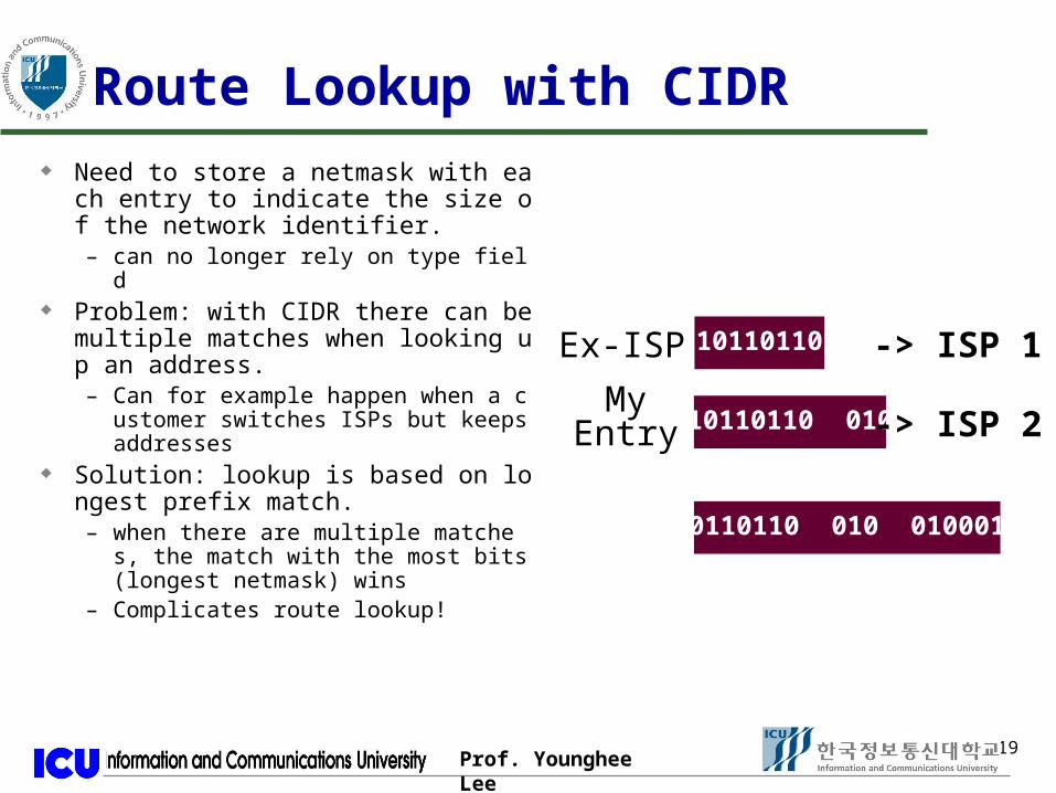
Route Lookup with CIDR Need to store a netmask with each en
try to indicate the size of the network identifier.– can no longer rely on type field
Problem: with CIDR there can be multiple matches when looking up an address.– Can for example happen when a custo
mer switches ISPs but keeps addresses
Solution: lookup is based on longest prefix match.– when there are multiple matches, the
match with the most bits (longest netmask) wins
– Complicates route lookup!
10110110
10110110 010
10110110 010 0100011
Ex-ISP
MyEntry
-> ISP 1
-> ISP 2

20Prof. Younghee Lee20
Shortcomings of CIDR
CIDR does not help with the large number of addresses that were already assigned before CIDR was introduced.
Many exceptions to CIDR addresses.– Customer receives a block of addresses and then moves
to a different ISP» Typically keeps the same addresses
– Many customers subscribe with several ISPs for redundancy
» Example: 45 Mbs with a primary ISP, and 5 Mbs with two backup ISPs
» Can only have one set of addresses

21Prof. Younghee Lee21
B IPB IP
NATs NAT maps (private source IP, source port) onto (public
source IP, unique source port)– reverse mapping on the way back– destination host does not know that is process is happening
Very simple working solution.– NAT functionality fits well with firewalls
Publ A IPPubl A IP
B IPB IP
A Port’A Port’ B PortB Port
Priv A IPPriv A IP
B IPB IP
A PortA Port B PortB Port
Publ A IPPubl A IP
B PortB Port
B IPB IP
Priv A IPPriv A IP
B PortB Port A PortA Port
A Port’A Port’
A
B

22Prof. Younghee Lee22
NAT Considerations NAT has to be consistent during a session.
– Set up mapping at the beginning of a session and maintain it during the session
– Recycle the mapping that the end of the session» May be hard to detect
NAT only work for certain applications.– Some applications (e.g. ftp) pass IP information in payload– Need application level gateways to do a matching translation
NAT has to be consistent with other protocols.– ICMP, routing, …
Many flavors of NAT exist.– Basic, network address port translation (NAPT), bi-directional,..
23Prof. Younghee Lee23
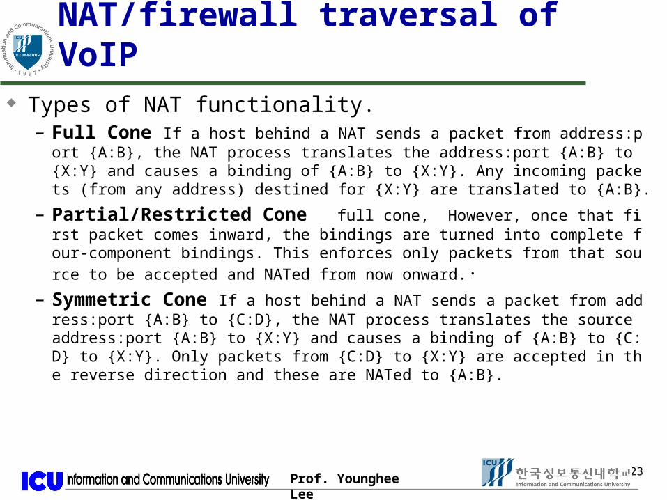
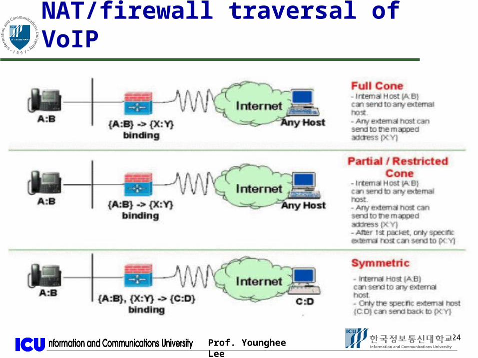
NAT/firewall traversal of VoIP Types of NAT functionality.
– Full Cone If a host behind a NAT sends a packet from address:port {A:B}, the NAT process translates the address:port {A:B} to {X:Y} and causes a binding of {A:B} to {X:Y}. Any incoming packets (from any address) destined for {X:Y} are translated to {A:B}.
– Partial/Restricted Cone full cone, However, once that first packet comes inward, the bindings are turned into complete four-component bindings. This enforces only packets from that source to be accepted and NATed from
now onward.· – Symmetric Cone If a host behind a NAT sends a packet from address:po
rt {A:B} to {C:D}, the NAT process translates the source address:port {A:B} to {X:Y} and causes a binding of {A:B} to {C:D} to {X:Y}. Only packets from {C:D} to {X:Y} are accepted in the reverse direction and these are NATed to {A:B}.
24Prof. Younghee Lee24
NAT/firewall traversal of VoIP

25Prof. Younghee Lee25
NAT/firewall traversal of VoIP NAT problem
– ‘Bindings’ can only be initiated by outgoing traffic.– Unsolicited incoming calls cannot be supported.
» Like incoming call of PABX can’t be translated without attendant.
26Prof. Younghee Lee26
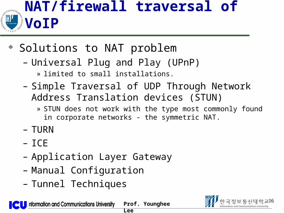
NAT/firewall traversal of VoIP
Solutions to NAT problem– Universal Plug and Play (UPnP)
» limited to small installations.
– Simple Traversal of UDP Through Network Address Translation devices (STUN)
» STUN does not work with the type most commonly found in corporate networks - the symmetric NAT.
– TURN– ICE– Application Layer Gateway – Manual Configuration – Tunnel Techniques

27Prof. Younghee Lee27
NAT/firewall traversal of VoIP
STUN– The STUN protocol enables a SI
P client to discover whether it is behind a NAT, and to determine the type of NAT.
» STUN server: “This is what I see as the source address and port”
TURN– Server that is inserted in the medi
a and signalling path. This TURN server is located either in the customers DMZ or in the Service Provider network.
» Increase latency and packet loss
28Prof. Younghee Lee28
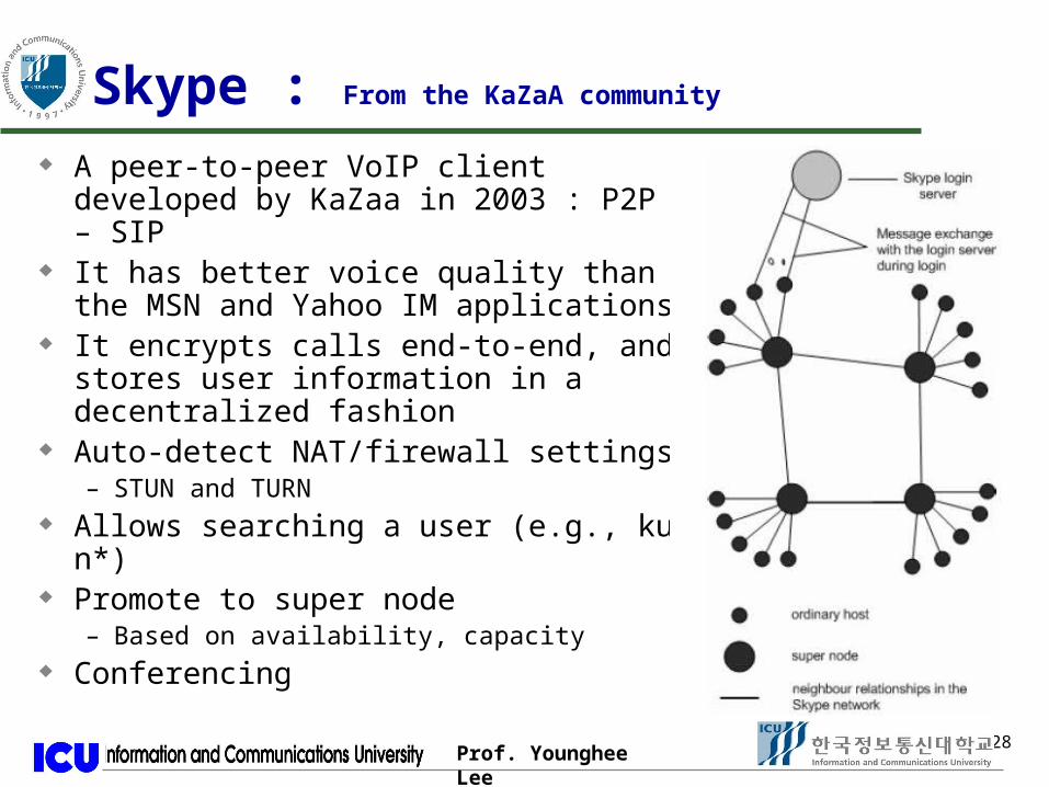
Skype : From the KaZaA community
A peer-to-peer VoIP client developed by KaZaa in 2003 : P2P – SIP
It has better voice quality than the MSN and Yahoo IM applications
It encrypts calls end-to-end, and stores user information in a decentralized fashion
Auto-detect NAT/firewall settings– STUN and TURN
Allows searching a user (e.g., kun*) Promote to super node
– Based on availability, capacity Conferencing

29Prof. Younghee Lee29
Kazaa FastTrack (aka Kazaa)
– Modifies the Gnutella protocol into two-level hierarchy» Hybrid of Gnutella and Napster
– Group leader» Nodes that have better connection to Internet» Act as temporary directory servers for other nodes in group» Maintains database, mapping names of content to IP address of its group member» Not a dedicated server; an ordinary server
– Bootstrapping node» A peer wants to join the network contacts this node.» This node can designate this peer as new bootstrapping node.
– Standard nodes» Connect to super nodes and report list of files» Allows slower nodes to participate
– Broadcast (Gnutella-style) search across Group leader peer; Query flooding– Drawbacks
» Fairly complex protocol to construct and maintain the overlay network» Group leader have more responsibility. Not truly decentralized » Still not purely serverless(Bootstrapping node is on “always up server”)
Overlay peer
Group leader peer
Neighboring relationshipsIn overlay network
30Prof. Younghee Lee30
IPv6
Initial motivation: 32-bit address space completely allocated by 2008.– => 128 bit address
Additional motivation:– header format helps speed processing/forwarding– header changes to facilitate QoS – new “anycast” address: route to “best” of several repli
cated servers
IPv6 datagram format: – fixed-length 40 byte header– no fragmentation allowed

31Prof. Younghee Lee31
IPv6 Header (Cont)
Priority: identify priority among datagrams in flowFlow Label: identify datagrams in same “flow.” (concept of“flow” not well defined).Next header: identify upper layer protocol for data
32Prof. Younghee Lee32
IPv6 Header: Flow Label
A flow: – A sequence of packets sent from a particular source to a
particular (unicast or multicast) destination for which the source desires special handling by the intervening routers.
» A flow may comprise multiple TCP connections: file transfer application» A single application may generate multiple flow: multimedia conferencing
one flow for audio, one for graphic window, .. With different requirements
Rules applied to the flow label– The source assigns a flow label to a flow. Chosen randomly in range 1
to 224-1.* a table with 224 (16 million) entries: memory burden.* on entry in the table per active flow: search the entire table=> hash table approach, CAM?
33Prof. Younghee Lee33
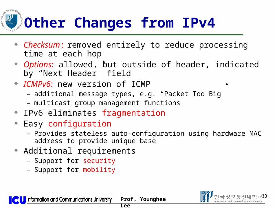
Other Changes from IPv4 Checksum: removed entirely to reduce processing time at each
hop Options: allowed, but outside of header, indicated by “Next
Header” field ICMPv6: new version of ICMP
– additional message types, e.g. “Packet Too Big”– multicast group management functions
IPv6 eliminates fragmentation Easy configuration
– Provides stateless auto-configuration using hardware MAC address to provide unique base
Additional requirements– Support for security– Support for mobility
34Prof. Younghee Lee34
Migration from IPv4 to IPv6
Interoperability with IPv4 is necessary for gradual deployment.
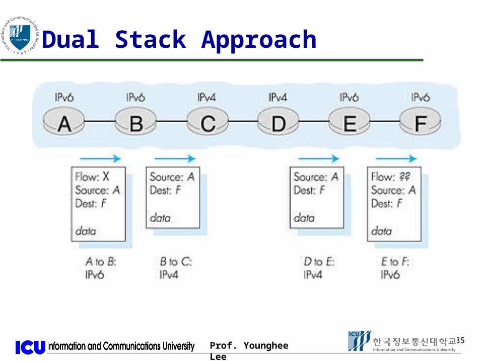
Two mechanisms:– dual stack operation: IPv6 nodes support both address types– tunneling: tunnel IPv6 packets through IPv4 clouds
Unfortunately there is little motivation for any one organization to move to IPv6.– the challenge is the existing hosts (using IPv4 addresses)– little benefit unless one can consistently use IPv6
» can no longer talk to IPv4 nodes
– stretching address space through address translation seems to work reasonably well
35Prof. Younghee Lee35
Dual Stack Approach

36Prof. Younghee Lee36
Tunneling
IPv6 inside IPv4 where needed
37Prof. Younghee Lee37
IPv6 Addresses A interface may have multiple unicast addresses.
– Allow subscriber that uses multiple access providers across the same interface to have separate addresses aggregated under each provider’s address space Longer Internet addresses allow for aggregating addresses by hierarchies of network, access provider, geography, corporation…
– smaller routing tables, faster table lookups Address types
– Unicast: an identifier for a single interface– Anycast: an identifier for a set of interface. Delivered to one of the interface(the “nearest” one for example)– Multicast: an identifier for a set of interfaces. Delivered to all interface.

38Prof. Younghee Lee38
IPv6 Stateless Autoconfiguration Local communication with no intervention
– Generate link-local address» corresponds to installed Ethernet network adapters. The last 64 bits of th
e IPv6 address is known as the interface identifier. It is derived from the 48-bit MAC address of the network adapter.
» Perform Duplicate Address Detection
– This looks like this:» FE80:0:0:0:XXXX:XXXX:XXXX:XXXX: prefix of FE80::/64» The X’s are the EUI-64 address.(extended unique identifier; 24 for company id)» They could be a random 64 bit address also.» The only requirement is that the address be unique.
– Start sending data Global communication with no stateful server Adds devices with no user configuration Stateful configuration: DHCP

39Prof. Younghee Lee39
Routing : source routing Source routing
– List entire path in packet Router processing
– Examine first step in directions– Strip first step from packet– Forward to step just stripped off
Advantages– Switches can be very simple and fast
Disadvantages– Variable (unbounded) header size– Sources must know or discover topology (e.g., failures)
Typical use– Ad-hoc networks (DSR)– Machine room networks (Myrinet)

40Prof. Younghee Lee40
Routing : Virtual Circuits/Tag Switching Connection setup phase
– Each router allocates flow ID on local link– VC connection id
Each packet carries connection ID Router processing
– Lookup flow ID – simple table lookup– Replace flow ID with outgoing flow ID– Forward to output port
Advantages– More efficient lookup (simple table lookup)– More flexible (different path for each flow)– QoS: reserve bandwidth at connection setup– Easier for hardware implementations
Disadvantages– Complex signalling to route connection setup request : stateful– More complex failure recovery – must recreate connection state
Typical uses– ATM – combined with fix sized cells– MPLS – tag switching for IP networks
41Prof. Younghee Lee41
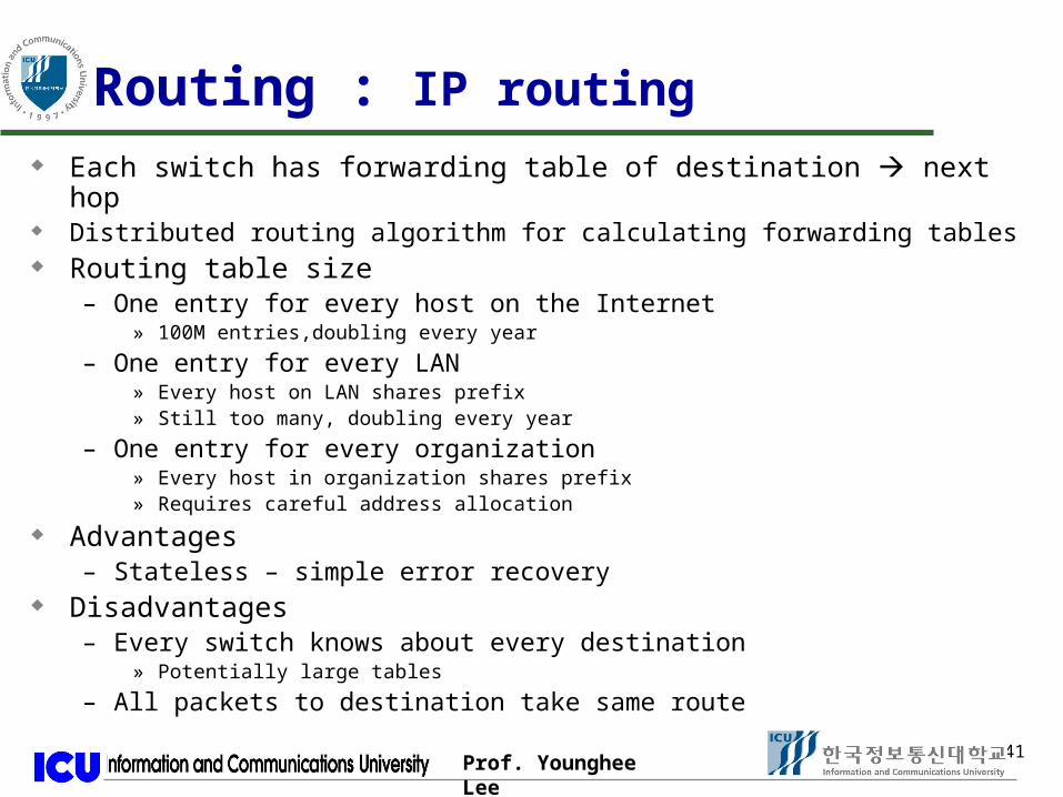
Routing : IP routing Each switch has forwarding table of destination next hop Distributed routing algorithm for calculating forwarding tables Routing table size
– One entry for every host on the Internet» 100M entries,doubling every year
– One entry for every LAN» Every host on LAN shares prefix» Still too many, doubling every year
– One entry for every organization» Every host in organization shares prefix» Requires careful address allocation
Advantages– Stateless – simple error recovery
Disadvantages– Every switch knows about every destination
» Potentially large tables
– All packets to destination take same route
42Prof. Younghee Lee42
Longest Prefix Match: is Harder than Exact Match
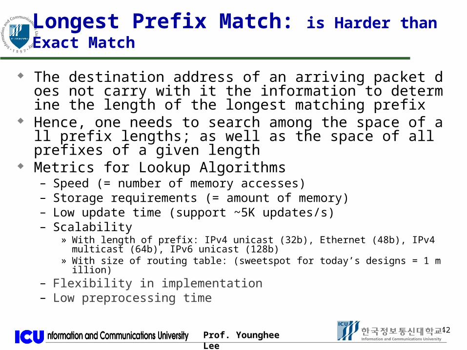
The destination address of an arriving packet does not carry with it the information to determine the length of the longest matching prefix
Hence, one needs to search among the space of all prefix lengths; as well as the space of all prefixes of a given length
Metrics for Lookup Algorithms– Speed (= number of memory accesses)– Storage requirements (= amount of memory)– Low update time (support ~5K updates/s)– Scalability
» With length of prefix: IPv4 unicast (32b), Ethernet (48b), IPv4 multicast (64b), IPv6 unicast (128b)
» With size of routing table: (sweetspot for today’s designs = 1 million) – Flexibility in implementation– Low preprocessing time

43Prof. Younghee Lee43
Longest Prefix Match
LPM in IPv4Use 32 exact match algorithms for LPM!
Exact matchagainst prefixes
of length 1
Exact matchagainst prefixes
of length 2
Exact matchagainst prefixes
of length 32
Network Address PortPriorityEncodeand pick
44Prof. Younghee Lee44
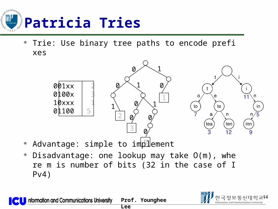
Patricia Tries Trie: Use binary tree paths to encode prefixes
Advantage: simple to implement Disadvantage: one lookup may take O(m), where
m is number of bits (32 in the case of IPv4)
001xx 2 0100x 310xxx 101100 5
0 1
0
1 0
1
1
0
0
0
0
2
3
5
1

45Prof. Younghee Lee45
Skip Count vs. Path Compression
Removing one way branches ensures # of trie nodes is at most twice # of prefixes; (case: trie containing a small number of very long strings)– Patricia tries
Using a skip count requires exact match at end and backtracking on failure path compression simpler
P1
P2
P3 P4
0
0
0 1
1
1
1
P1
P2
P3 P4
0
0
0 1
(Skip count) Skip 2
or
11 (path compressed)
1
46Prof. Younghee Lee46
Fast Longest Prefix Match
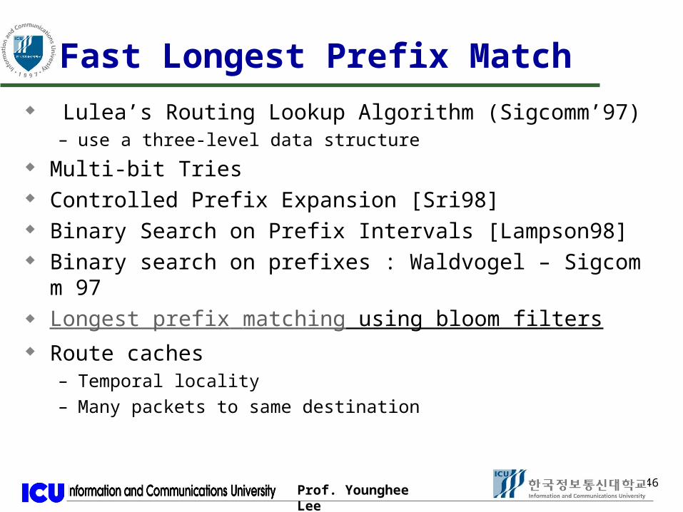
Lulea’s Routing Lookup Algorithm (Sigcomm’97)– use a three-level data structure
Multi-bit Tries Controlled Prefix Expansion [Sri98] Binary Search on Prefix Intervals [Lampson98] Binary search on prefixes : Waldvogel – Sigcomm 97 Longest prefix matching using bloom filters Route caches
– Temporal locality– Many packets to same destination

47Prof. Younghee Lee47
Fast Longest Prefix Match
Content addressable memory (CAM)– Hardware based route lookup– Input = tag, output = value associated with tag– Requires exact match with tag
» Multiple cycles (1 per prefix searched) with single CAM
» Multiple CAMs (1 per prefix) searched in parallel
– Ternary CAM» 0,1,don’t care values in tag match
» Priority (I.e. longest prefix) by order of entries in CAM

48Prof. Younghee Lee48
Performance Comparison: Complexity
Algorithm Lookup Storage Update
Binary trie W NW W
Patricia W2 N W
Path-compressed trie W N W
Multi-ary trie W/k N*2k -
LC trie W N -
Lulea - - -
Binary search on trie levels logW NlogW -
Binary search on intervals log(2N) N -
TCAM 1 N W

49Prof. Younghee Lee49
Performance Comparison
Algorithm Lookup (ns) Storage (KB)
Patricia (BSD) 2500 3262
Multi-way fixed-stride optimal trie (3-levels) 298 1930
Multi-way fixed-stride optimal trie (5-levels) 428 660
LC trie - 700
Lulea 409 160
Binary search on trie levels 650 1600
6-way search on intervals 490 950
Lookups with direct access 15-60 9-33 * 1000
TCAM 15-20 512

50Prof. Younghee Lee50
Packet classification
Packet classification – The process of categorizing packets into “flows” in an In
ternet router– All packets belonging to the same flow obey a predefine
d rule and are processed in a similar manner by the router
Flow-aware router: keeps track of flows and perform similar processing on packets in a flow– Non best effort services, firewalls, QoS
Flow-unaware router (packet-by-packet router): treats each incoming packet individually

51Prof. Younghee Lee51
Example of Classification Rules Access-control in firewalls
– Deny all e-mail traffic from ISP-X to Y Policy-based routing
– Route IP telephony traffic from X to Y via ATM Differentiate quality of service
– Ensure that no more than 50 Mbps are injected from ISP-X Committed Access Rate (rate limiting)
– Rate limit WWW traffic from sub interface#739 to 10Mbps

52Prof. Younghee Lee52
Complexity: Hard Problem
N rules and k header fields for k > 2– O(log Nk-1) time and O(N) space– O(log N) time and O(Nk) space
How many rules?– Largest for firewalls & similar 1700– Diffserv/QoS much larger 100k (?)

53Prof. Younghee Lee53
Multi-field Packet Classification
Given a classifier with N rules, find the action associated with the highest priority rule matching an incoming packet.
Example: packet (5.168.3.32, 152.133.171.71, …, TCP)
Field 1 Field 2 … Field k ActionRule 1 5.3.90/21 2.13.8.11/32 … UDP A1
Rule 2 5.168.3/24 152.133/16 … TCP A2
… … … … … …
Rule N 5.168/16 152/8 … ANY AN

54Prof. Younghee Lee54
Special processing
Control
Datapath:per-packet processing
Routing lookup
Flow-aware Router: Basic Architectural Components
Routing, resource reservation, admission control, SLAs
Packet classification
Switching
Scheduling
55Prof. Younghee Lee55
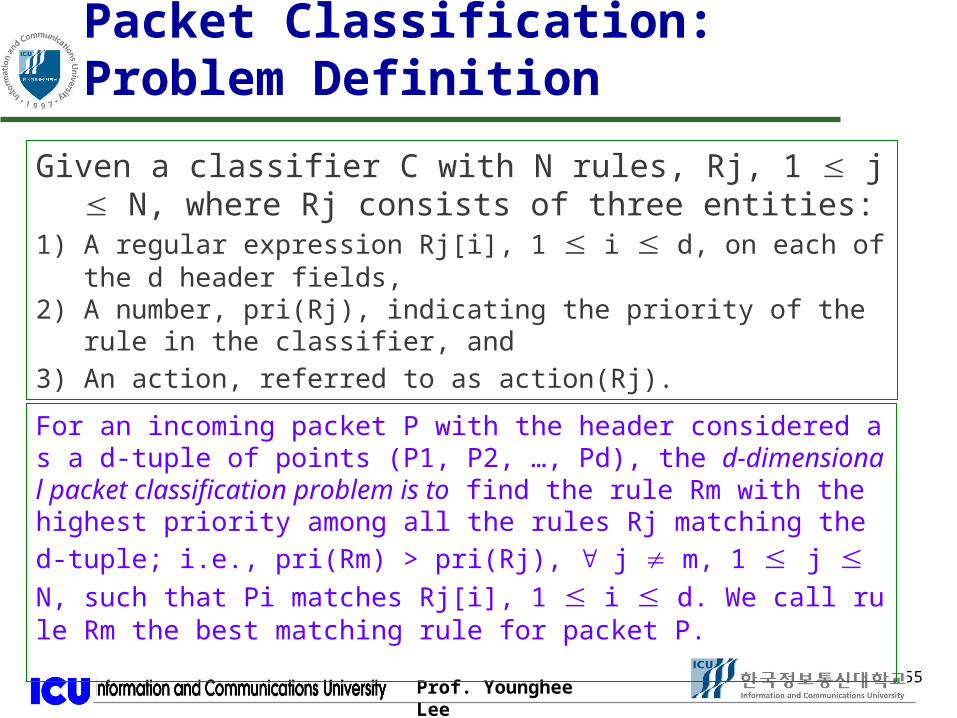
Packet Classification: Problem Definition
Given a classifier C with N rules, Rj, 1 j N, where Rj consists of three entities:
1) A regular expression Rj[i], 1 i d, on each of the d header fields, 2) A number, pri(Rj), indicating the priority of the rule in the classifier, a
nd3) An action, referred to as action(Rj).
For an incoming packet P with the header considered as a d-tuple of points (P1, P2, …, Pd), the d-dimensional packet classification problem is to find the rule Rm with the highest priority among all the rules Rj matching the d-tuple; i.e., pri(Rm) > pri(Rj), j m, 1 j N, such that Pi matches Rj[i], 1 i d. We call rule Rm the best matching rule for packet P.

56Prof. Younghee Lee56
Example 4D classifier
Rule L3-DA L3-SA L4-DP L4-PROT Action
R1 152.163.190.69/255.255.255.255
152.163.80.11/255.255.255.255
* * Deny
R2 152.168.3/255.255.255
152.163.200.157/255.255.255.255
eq www udp Deny
R3 152.168.3/255.255.255
152.163.200.157/255.255.255.255
range 20-21 udp Permit
R4 152.168.3/255.255.255
152.163.200.157/255.255.255.255
eq www tcp Deny
R5 * * * * Deny

57Prof. Younghee Lee57
Example Classification Results
Pkt Hdr
L3-DA L3-SA L4-DP L4-PROT Rule, Action
P1 152.163.190.69 152.163.80.11 www tcp R1, Deny
P2 152.168.3.21 152.163.200.157 www udp R2, Deny
58Prof. Younghee Lee58
Classification is a Generalization of Lookup
Classifier = routing table One-dimension (destination address) Rule = routing table entry Regular expression = prefix Action = (next-hop-address, port) Priority = prefix-length

59Prof. Younghee Lee59
Example Two-dimension space, i.e., classification based on two fields Complexity depends on the layout, i.e., how many distinct
regions are created
60Prof. Younghee Lee60
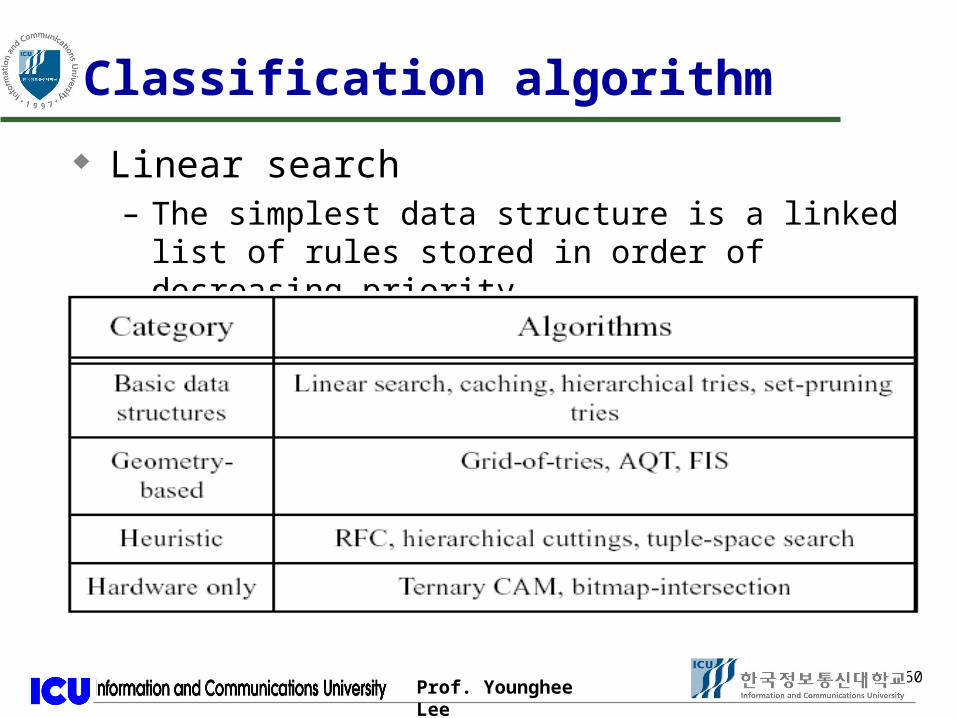
Classification algorithm
Linear search– The simplest data structure is a linked list of rules
stored in order of decreasing priority
61Prof. Younghee Lee61
Recursive Flow Classification [Gupta99]
Difficult to achieve both high classification rate and reasonable storage in the worst case
Real classifiers exhibit structure and redundancy
A practical scheme could exploit this structure and redundancy
Observations:

62Prof. Younghee Lee62
RFC: Classifier Dataset
793 classifiers from 101 ISP and enterprise networks with a total of 41505 rules.– Classifier (policy database)
40 classifiers: more than 100 rules. Biggest classifier had 1733 rules.
Maximum of 4 fields per rule: source IP address, destination IP address, protocol and destination port number.

63Prof. Younghee Lee63
RFC: Problem formulation:
– Map S bits (i.e., the bits of all the F fields) to T bits (i.e., the class identifier) Main idea:
– Create a 2S size table with pre-computed values; each entry contains the class identifier
» Only one memory access needed
– …but this is impractical require huge memory– Use recursion: trade speed (number of memory accesses) for memory footprint

64Prof. Younghee Lee64
The RFC Algorithm
At each stage the algorithm maps one set of values to a smaller set– A set of memories return a value shorter than the index of
the memory access
Split the F fields in chunks1. Use the value of each chunk to index into a table
Indexing is done in parallel
2. Combine results from previous phase, and repeat
3. In the final phase we obtain only one value that is action

65Prof. Younghee Lee65
Chunking of a Packet
Source L3 Address
Destination L3 Address
L4 protocol and flags
Source L4 port
Destination L4 port
Type of Service
Packet Header
Chunk #0
Chunk #7

66Prof. Younghee Lee66
The RFC Algorithm

67Prof. Younghee Lee67
Complete Example
indx=c02*6+c03*3+c05
indx=c10*5+c11

68Prof. Younghee Lee68

69Prof. Younghee Lee69
Choice of Reduction Tree
3
2
1
0
5
4
Number of phases = P = 310 memory accesses
3
2
1
0
5
4
Number of phases = P = 411 memory acceses

70Prof. Younghee Lee70
RFC: Classification Time
Pipelined hardware: 30 Mpps (worst case OC192) using two 4Mb SRAMs and two 64Mb SDRAMs at 125MHz.
Software: (3 phases) 1 Mpps in the worst case and 1.4-1.7 Mpps in the average case. (average case OC48) [performance measured using Intel Vtune simulator on a windows NT platform]

71Prof. Younghee Lee71
RFC: Pros and Cons
Advantages
Exploits structure of real-life classifiersSuitable for multiple fieldsSupports non-contiguous masksFast accesses
Disadvantages
Depends on structure of classifiersLarge pre-processing timeIncremental updates slowLarge worst-case storage requirements
72Prof. Younghee Lee72
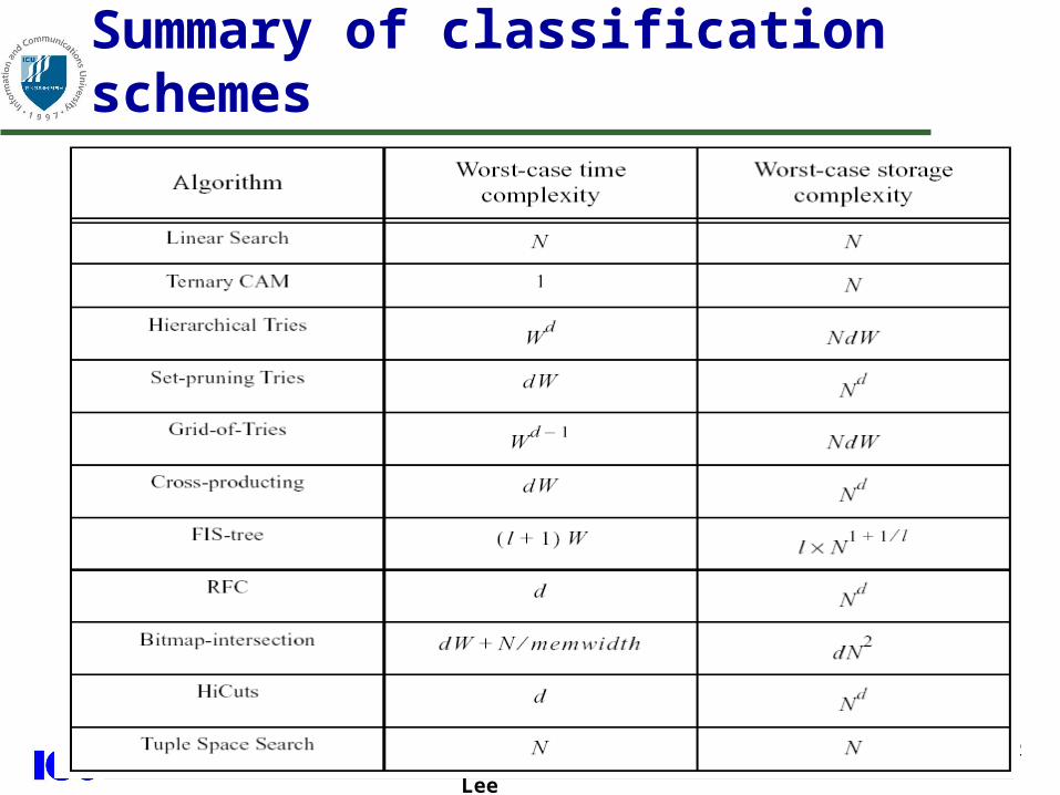
Summary of classification schemes

73Prof. Younghee Lee73
Lookup/Classification Chip Vendors – Switch-on– Fastchip– Agere– Solidum– Siliconaccess– TCAM vendors: Netlogic, Lara, Sibercore, Mosaid, Kl
si etc.
Packet classification still an area of active research
Summary of classification schemes