DI

SC

US

SI

ON

P

AP

ER

S

ER

IE

S

Forschungsinstitut zur Zukunft der ArbeitInstitute for the Study of Labor

Productivity, Wages, and Marriage:The Case of Major League Baseball

IZA DP No. 5695

May 2011

Francesca CornagliaNaomi E. Feldman

Productivity, Wages, and Marriage: The Case of Major League Baseball

Francesca Cornaglia Queen Mary, University of London

and IZA

Naomi E. Feldman Ben-Gurion University

Discussion Paper No. 5695 May 2011

IZA

P.O. Box 7240 53072 Bonn

Germany

Phone: +49-228-3894-0 Fax: +49-228-3894-180

E-mail: iza@iza.org

Any opinions expressed here are those of the author(s) and not those of IZA. Research published in this series may include views on policy, but the institute itself takes no institutional policy positions. The Institute for the Study of Labor (IZA) in Bonn is a local and virtual international research center and a place of communication between science, politics and business. IZA is an independent nonprofit organization supported by Deutsche Post Foundation. The center is associated with the University of Bonn and offers a stimulating research environment through its international network, workshops and conferences, data service, project support, research visits and doctoral program. IZA engages in (i) original and internationally competitive research in all fields of labor economics, (ii) development of policy concepts, and (iii) dissemination of research results and concepts to the interested public. IZA Discussion Papers often represent preliminary work and are circulated to encourage discussion. Citation of such a paper should account for its provisional character. A revised version may be available directly from the author.

IZA Discussion Paper No. 5695 May 2011

ABSTRACT

Productivity, Wages, and Marriage: The Case of Major League Baseball*

Using a sample of professional baseball players from 1871–2007, this paper aims at analyzing a longstanding empirical observation that married men earn significantly more than their single counterparts holding all else equal (the “marriage premium”). Baseball is a unique case study because it has a long history of statistics collection and numerous direct measurements of productivity. Our results show that the marriage premium also holds for baseball players, where married players earn up to 16 percent more than those who are not married, even after controlling for selection. The results hold only for players in the top third of the ability distribution and post 1975 when changes in the rules that govern wage contracts allowed for players to be valued closer to their true market price. Nonetheless, there do not appear to be clear differences in productivity between married and nonmarried players. We discuss possible reasons why employers may discriminate in favor of married men. JEL Classification: J31, J44, J70 Keywords: marriage premium, wage gap, productivity, baseball Corresponding author: Francesca Cornaglia School of Economics and Finance Queen Mary, University of London Mile End Road, London E1 4NS United Kingdom E-mail: f.cornaglia@qmul.ac.uk

* We thank Kermit Daniel and Sandy Korenman for providing their dissertations, David Yermack for providing contract data, Lucia Dunn and Charlie Mullin for providing player MRP data, Jerome Adda, Josh Angrist, John Bound, Todd Kaplan, Joel Slemrod, Chris Tyson, Oscar Volij, Jason Winfree and seminar participants from Ben-Gurion University, Federal Reserve Board, Hebrew University of Jerusalem, LSE, MIT, Tel-Aviv University, Tulane University, University of Chicago, UIUC, and University of Michigan for comments. We are also indebted to Jim Gates, Library Director of the Hall of Fame for providing unfettered access to the library’s archives and resources, Bill Deane and his excellent team of freelance baseball researchers and David Katz, avid White Sox fan. We are grateful to the ESRC for funding [RES-000-22-3267]. The findings and views reported in this paper are those of the authors and should not be attributed to the above individuals or organizations. All errors are our own.

1 Introduction

The effect of marriage on wages has been long debated in the economic literature. The main conclusion

in standard cross-sectional log wage regressions is that married men are estimated to earn a “marriage

premium”–roughly 10 - 40 percent higher wages than their single counterparts. There are a number of

proposed explanations for this finding, the first of which is endogenous selection. In particular, selection

may be based on unobserved characteristics that are correlated with both marital status and productivity.

Additionally, the positive correlation between marriage and wages may be due to reverse causality where

men with high wages or high wage growth tend to be more successful in the marriage market. In contrast to

this, another line of explanations take the view that marriage has a causal effect on wages. This may be due to

employer discrimination (married men are seen as more “stable”) or, as many have concluded, productivity

differences due to specialization between household and non-household work afforded by marriage. Because

men are freer to concentrate on non-household work, they therefore become more productive workers. The

marriage premium is of particular interest for analyzing gender-based discrimination in labor markets, as the

male marital pay premium accounts for about one-third of estimated gender-based wage discrimination in the

United States (Neumark 1988). We investigate the relationship between wages, marriage and productivity

using data on professional baseball players. Our analysis will provide evidence as to whether there exists

some basis to this observed discrimination once productivity is taken into account.

There are a number of aspects to our research that improve upon previous studies. First and foremost,

a notable feature of our analysis is that we use direct objective measures of productivity. Specifically, we

consider professional baseball players, making use of data we hand collected from the National Baseball

Hall of Fame and Museum data depositories and merged with productivity measures from Sean Lahman’s

Baseball Archive database. This rich dataset allows us to directly assess whether there is a relationship

between marriage and productivity as opposed to only an indirect linkage via wages. The fact that we make

use of objective productivity measures is, to our knowledge, novel in the analysis of the marriage premium.1

In addition, access to these direct productivity measures helps to mitigate a number of potential problems

that have plagued the literature. We discuss these problems more in depth in Section 2, however, to provide

one example, potential wives in standard data sets may have more information than the econometrician

1A few papers have used subjective productivity measures, such as supervisor ratings. See Section 2.

2

regarding the future earning capacity of the potential husband and those with high earning capacity may

be more likely to marry. Thus, what would appear to be marriage’s effect on wages is, in fact, the reverse

relationship. Our productivity measures likely serve as a sufficient statistic for future earning capacity and

we can therefore control for this issue in any analysis.

As previous studies have found, our results also show that marriage and wages are positively correlated.

Married men earn roughly between 16 percent more than their single counterparts. However, this result

holds only for the top one-third of the ability distribution and post-1975 when strict rules governing con-

tracts were overturned and wages became free to respond to market forces. In contrast to the wage results,

marriage appears to have no statistically significant effect on productivity using a variety of measurements

and subsamples of the data. Thus, while marriage appears to impact wages, its primary mechanism does

not appear to be through its impact on productivity. In fact, controlling for productivity in a wage equation

shows that the statistically significant effect of marital status remains. We hypothesize that an impact on

wages may be due to a number of nontangible aspects of marriage that are not necessarily captured by our

direct productivity measures such as stability, leadership, negotiation skills and popularity that possibly lead

employers to discriminate in their favor. We provide some evidence in support of this, where marriage has

a negative effect on the variance of our productivity measures for certain players (and a positive effect for

others) and a positive effect on the extraction of economic rent. That is, the gap between marginal revenue

product and wages is smaller for married players. In addition, we also find that the team level fraction of

married players is positively correlated with ballpark attendance and team wins.

2 Literature

The observation that married men earn more than their single counterparts has been well documented

using many different datasets and across numerous time periods and countries. There have been two main

empirical approaches in the marriage premium literature: studies that make use of cross-sectional data

and/or those that make use of panel data (see Ribar (2004) for a review of the methodologies). Generally

speaking, cross-sectional results (for example, Bellas (1992), Blau and Beller (1988), Blackburn and Ko-

renman (1994), Chun and Lee (2001), Duncan and Holmlund (1983), Hewitt, Western and Baxter (2002),

3

Hill (1979), Kenny (1983), Korenman and Neumark (1991), Krashinsky (2004), Nakosteen and Zimmer

(1987), Schoeni (1995)) have found clear evidence of a marriage premium.2 Attempts are made to control

indirectly for cross-sectional variation in ability but cannot dismiss the interpretation that the results are

driven by unobserved individual characteristics and the effect is overstated due to selection into marriage.3

As such, many of the papers also include fixed-effects panel data analyses that attempt to correct for this

bias (for example, Bardasi and Taylor (2005), Cornwell and Rupert (1995, 1997), Datta Gupta, Smith, and

Stratton (2005), Duncan and Holmlund (1983), Ginther and Zavodny (2001), Hersch and Stratton (2000),

Korenman and Neumark (1991), Krashinsky (2004), Loughran and Zissimopoulos (2009), Neumark (1988),

Richardson (2000), Rogers and Stratton (2005) and Stratton (2002)). Panel data results have been mixed,

some studies find no statistically significant effect of marriage on wages while others find a residual positive

effect. These studies generally conclude that there is some causal effect of marriage on wages, whether it is

on productivity or merely discrimination is often unresolved.

All of these studies, both cross sectional and panel data, typically include a measure of log wages for the

dependent variable and a binary indicator for marital status, some variation of marital status (never married,

cohabitation, divorced) or length of marriage along with other demographic controls such as age, education,

experience and race. Cross-sectional studies have typically estimated a marriage premium ranging between

10 - 40 percent. While most panel data estimates have confirmed this positive correlation between wage and

marital status, some have found the effect to be indistinguishable from zero (e.g. Gray 1997).

We characterize broadly the main explanations of the marriage premium into issues of selection and

issues of causality. Under selection, we have the following explanations: (1) men with high unobserved

ability exhibit characteristics that are more likely to be found attractive by both employers and potential

spouses (for example, stability, industriousness, physical appearance, etc.); (2) married men (or men who

are likely to marry) may tend to sort into professions that have higher wages and less non-pecuniary benefits;

and (3) reverse causality–men with high wages or wage growth may find themselves facing an improved pool

2A number of papers [see, for example, Cohen (2002), Loh (1996), Richardson (2000)] have also considered cohabitation statusas separate from never-married and typically find a cohabitation premium that is less than the marriage premium but nonethelesspositive and significant. Stratton (2002) also considered cohabiters but found that once taking into unobservable individual effects,the premium disappears.

3Krashinsky (2004) and Antonovics and Town (2004) have used first differenced data on twins to account for unobserved ability.The first study finds that the marriage premium is statistically indistinguishable from zero among twin pairs while the latter findsthat the marriage premium remains positive and significant.

4

of potential spouses and therefore more likely to marry. Under causality, we have the following explanations:

(1) specialization between household and nonhousehold work between the spouses and, relatedly, spousal

investment in augmentation skills (see Section 3). In other words, the wife invests in activities that cause

the husband to be more productive in the workplace (Becker, 1981); and (2) employer discrimination for

a given level of productivity. Employers that exhibit a preference for married workers are not necessarily

discriminating against single workers if married workers are more productive. Yet, even when controlling

for current productivity, employers may still prefer married workers because they may be more stable, less

mobile, exhibit leadership skills, among other reasons.

The first two explanations under selection have been well addressed in the literature. As we mentioned,

in order to account for unobserved ability, researchers have used panel data with fixed effects models, under

the assumption of time-constant ability. An example is the analysis done by Korenman and Neumark (1991)

using data from the National Longitudinal Survey of Young Men (NLSY-M). They find that selection on the

basis of fixed unobservable characteristics accounts for less than 20 percent of the observed wage premium.

In a later contribution, Bardasi and Taylor (2005), using data from the British Household Panel (BHPS),

show that when moving form OLS to FE the marriage premium falls from 0.09 to 0.02. A zero marriage

premium when taking into account individual effects is also found in earlier studies, such as Cornwell and

Rupert (1995 and 1997) and Gray (1997), and in more recent contributions like that by Krashinsky (2004).

A number of papers have found evidence of sorting (among these Petersen, Penner and Hogsnes (2006) and

Korenman and Neumark (1991)). They have found that the marriage premium disappears once controlling

for profession.

Consistent with past literature, we are able to estimate our model using standard fixed effects estimation

due to the panel nature of our data. Moreover, given that our entire sample is in the same profession, the

sorting issue is of significantly less concern, though, it is true that the type of man that selects into profes-

sional baseball is not necessarily representative of men in general. The third explanation under selection

issues has received considerably less attention in the literature. To our knowledge, the sole paper to con-

sider the problem of reverse causality is Korenman (1988). Korenman provides evidence that wages are not

positively correlated with future changes in marital status, a fact that makes the reverse causality argument

less of a concern. Because we are able to control for productivity, it is unlikely that the potential spouse has

5

more information regarding the future earning potential of the player than the econometrician in this case.

Moreover, to the extent that productivity (or a change in productivity) does not fully explain wages (or a

change in wages), conditional on a number of other controls, we are able to make use of institutional details

in the setting of contracts that impact wages and wage growth but are arguably uncorrelated with marital

status (see Section 8.2).4

The causality explanations have, for the most part, received indirect support in the literature. The afore-

mentioned papers that found a residual effect of marriage on wages, after controlling for individual fixed

effects and other controls, generally interpret the finding of a statistically significant coefficient on marital

status as the causal effect of marriage on wage that arises from specialization. Attempts have been made to

test this causal explanation by controlling for things like hours worked by the wife. The idea is that marriage

allows a man to focus on non-household labor while the wife engages in traditional household labor. Evi-

dence is mixed. Many of the papers that have contributed to this literature, for example, Daniel (1995), Gray

(1997), Chun and Lee (2001), and Bardasi and Taylor (2005) find a wage penalty associated with wife’s

labor hours. Hersch and Stratton (2000), on the other hand, using data from the National Survey of Fam-

ilies and Households, find that household specialization does not seem to be responsible for the marriage

premium. Along the same line are the results by Loh (1996). He finds no evidence that wives’ labor force

participation underlies the return to marriage for men. Similar findings are obtained by Jacobsen and Ray-

ack (1996) using the Panel Study of Income Dynamics (1984-1989), and by Hotchkiss and Moore (1999)

using the Current Population Survey. Daniel (1993) using the NLSY highlights some racial differences in

the marriage premium, in particular he finds that it is inversely related to the wife’s hours of work only for

white men.

There are a number of papers that make some use of productivity measures and are therefore particu-

larly relevant for our study. Korenman and Neumark (1991) use data from a personnel file of a large U.S.

manufacturing firm from 1976. What is useful from this data is that is contains supervisor performance

4Another take on this issue is that it is less of problem in our particular setting than it would be with more standard panel datasets. For close to the past 40 or so years, baseball players have been extremely high earning relative to the population. Medianwages as well as the MLB minimum wage have increased exponentially in the modern period. Thus, the question is whetherplayers see marginal improvements in their spousal applicant pool and probability of marrying as their careers progress and wagesincrease from already high levels to even higher levels? Or, does the biggest improvement in the applicant pool and the probabilityof marrying come when expectations of entering MLB pass a certain threshold? We tend to believe the latter but do not entirelydismiss the former argument and therefore address the concerns raised.

6

ratings that provide a measure of worker productivity aside from the worker’s wage. The authors attempt to

measure productivity, albeit somewhat subjectively, and find that nearly all of the marriage premium (from

23 percent to 2 percent) disappears once adding pay grade and performance rating dummies. Mehay and

Bowman (2005) use administrative data on male U.S. Naval officers in technical and managerial jobs to

explore the effect of marriage on several job performance measures (e.g. promotion outcomes and annual

performance reviews). They find that married men receive higher performance ratings and are more likely

to be promoted than non married men (the result is robust to selection arising from quit decisions). These

contributions, while using direct measures of productivity, nonetheless, use subjective measures that are

potentially affected by reporting biases. It is possible, in fact, plausible that supervisors simply perceive

married men to be more productive workers and therefore give them higher performance ratings or grant

them more frequent promotions.

The productivity measures we use, alternatively, are objective measures based on exogenous, histori-

cal measures of productivity. These objective measures of productivity have been extensively used in the

baseball literature mainly for analyzing the role of labor contracts and more generally for studying the

specificities of the baseball labor market (Kahn, 1993; Macdonald and Reynolds, 1994; Rottenberg, 1956;

Scully, 1974; Zimbalist, 2003), investigating discrimination issues (Andresen and La Croix, 1991; Depken

and Ford, 2006; Gwartney and Haworth, 1974; Hanssen and Andersen, 1999; Hill and Spellman, 1984;

Lanning, 2010; Nardinelli and Curtis, 1990) and the role of strategic management (Porter and Scully, 1982;

Smart, Winfree and Wolfe, 2008).

3 A Model of the Marriage Premium

There was one big glitch: these sorts of calculations could value only past performance. No matter how

accurately you value past performance, it was still an uncertain guide to future performance. Johnny

Damon (or Terrence Long) might lose a step. Johnny Damon (or Terrence Long) might take to drink or

get divorced.

(Moneyball: The Art of Winning an Unfair Game, p. 136)

It was better than rooming with Joe Page.

7

Joe DiMaggio’s response when asked if his marriage to Marilyn Monroe was good for him.5

In this section we sketch a model and provide intuition for the effect that marriage has on spousal

wage.6 We assume here that marriage impacts salary through two channels. First, it impacts salary indirectly

through its positive causal effect on productivity that occurs because the wife engages in particular actions

that impact the productivity of the husband. The main purpose of this involvement is to provide her husband

with uncluttered time. For example, a wife may engage in home production such as cooking, cleaning and

childcare so that her husband can focus on his career with fewer distractions. She may also provide career

advice and moral support or simply allow him extra sleep.

Second, we also allow for marriage to impact wages directly as opposed to indirectly via productivity.

These direct influences can take on a number of forms that may lead employers to discriminate in favor of

married men. For example, a wife may impact her husband’s popularity and visibility through public image

(for example, hosting formal dinners, participating in public events, charity events, etc.) or marriage may

increase a man’s stability, reliability (among other characteristics) that in turn make him a better teammate.

A professional athlete’s career is accompanied by numerous formal and informal expectations and therefore

not only is the management of the athlete’s self-image important, but that of their wives is crucial too. The

wife represents her husband to the public, providing a visible link between the worlds of work and family

(Crute, 1981).7 In sum, through these two channels, the wife is able to take actions that make each unit

of her husband’s time in the market more effective and/or more profitable. All of these wage enhancing

activities are subsumed under the heading of “augmentation activities.”

Thus, a husband’s wage is a function of direct augmentation activities and productivity while produc-

tivity is, in turn, a function of indirect augmentation activities and innate ability. Both are also functions of

other demographic characteristics such as age and race as well as variables such as experience. We assume

further that these variables affect men of different ability levels differently. We can therefore model wages

5Granted, DiMaggio was retired by the time he married Monroe, whom, by any standards, was not a typical ballplayer’s wife.6Our model is inspired by Daniel (1993). Without loss of generality, we consider a marriage premium only for the husband

though, it is more accurately described as a marriage premium for the higher earning spouse.7"A wife’s look and behavior...can even affect her husband’s baseball career. You are part of the package, and if you don’t look

the part, well, some are going to notice." (Gmelch and San Antonio, 2001).

8

and productivity as follows:

S = S(P,τ,X) and

P(ρ, t,X), (1)

where S is yearly salary, τ is the direct and t the indirect activities that impact spousal wages, P represents

productivity, and X is a vector of other variables that impact wages and productivity, such as age, race, and

experience, among others. Ability is captured by ρ , where higher numbers represent higher innate ability.

We focus on the particular case of our model where wives invest solely in augmentation activities and

do not work. In addition, leisure is predetermined for both spouses in order to abstract from the labor-leisure

decision.8 Thus, total available time for the wife (T ) is divided between the two augmentation activities.

The zero labor hours restriction also has anecdotal, as well as more formal support. The demands of a pro-

fessional baseball career do not facilitate a stable lifestyle where wives could invest in their own careers.

The far majority of wives of MLB players do not work outside of the home as they run the households.9

Moreover, with rare exception, MLB players earn wages that are much higher that any wage their wives

could earn, which discourages wives’ participation in the labor market.10 11 There are a number of interest-

ing implications from this simple model. For instance, suppose that two men have different ability but equal

productivity, that is, ρ1 > ρ2 but P(ρ1, t1,X) = P(ρ2, t2,X). Under the assumption of monotonicity of P(.),

t1 < t2 and therefore τ1 = T − t1 > T − t2 = τ2. In words, conditional on equal productivity, the wives of

higher ability men spend less time on indirect and more time on direct augmentation than the wives of lower

ability men. As a result, S(P(ρ1, t1,X),T − t1,X) = S(P(ρ2, t2,X),T − t1,X) > S(P(ρ1, t1,X),T − t2,X) by

8The assumption of setting labor hours equal to zero for the wife would also arise endogenously from the model given sufficientlylarge husband wages relative to wives.

9Source: email correspondence with Denise Schmidt, attorney for the Baseball Wives Charitable Foundation (BWCF).10Blau and Kahn (2007) and Wolfram and Leber Herr (2008) present interesting evidence that wives are less likely to participate

in the labor force the higher is the husband’s wage even taking into account that high earning men tend to be married to high earningwomen. Inspired by the Wolfram and Leber Herr findings an on-line article noted that “...Men who are in the upper ranks of theirprofession with stay-at-home-wives earn 30 percent more than men who are married to women who work. Those men who want toreach the highest rungs of their career and earn the most money often need a stay-at-home wife to take care of all other aspects oftheir life, including raising a family.” [“MBA Moms Most Likely to Opt Out,” Bloomberg Business Week, August 21, 2008.]

11An anonymous CEO “...allegedly stated that his wife should not work but rather should stay home and run the household, hosthis parties and mother his children since any wage she would make would essentially be insignificant.” [“If Vikram Pandit is oustedfrom Citi will his wife Swati divorce him?”, Divorce Saloon, The Global 24/7 Divorce and Family Law Blog, July 2, 2010.]

9

monotinicity of S(.). Another way to think about it is as follows: in the case of differing abilities but equal

time spent on indirect augmentation, that is ρ1 > ρ2 and t1 = t2, we have P(ρ1, t1,X) > P(ρ2, t2,X). Provided

P(.) is quasiconcave, the marginal impact of an increase in t is decreasing in ability.

Families maximize utility subject to standard budget constraints

maxt

u(C) subject to

C−S(P(ρm, t f ,Xm),T − t f ,Xm)+Y ≤ 0,

τf + t f ≤ T, (2)

C,τ f , t f ≥ 0,

where, in addition to the variables described above, C is consumption, and Y is nonwage income. The

indexes m and f represent male and female, respectively.

The first order condition with respect to t is as follows:

S1(P,T − t f ,X) ·P2(ρm, t f ,Xm)≤ S2(P,T − t f ,Xm) (3)

where equality holds in the case of an interior solution (that is, the spouse does not desire to spend more

than T hours on augmentation activities). The left hand side of equation (3) reflects the return to indirect

augmentation while the right hand reflects the implied return on direct augmentation. For a given value of

ρ , the wife equates the marginal value of one more unit invested in τ f with the marginal value of one more

unit invested in t f . In this model, both spouses are fully invested in one career. Wives form a work pattern

that Papanek (1973, p.90) has labeled the “two person career,” characterized by “...a combination of formal

and informal institutional demands ... (are) placed on both members of a married couple of whom only the

man is employed by the institution.”

10

4 A Primer on Baseball

Professional athletes are a subsample of the population where direct measurements of productivity are

observable. In contrast to other team sports, such as basketball and soccer, performance in baseball is

directly quantifiable and with a number of measures that are relatively independent of the actions of the

player’s teammates. Moreover, while there have been changes in the rules over time, relatively speaking,

baseball is a fairly stable sport with a long history of uniform player statistics collection. The current typical

baseball season is 162 games and runs from early April until early October, followed by the post-season

tournament in October that culminates with the World Series. The regular season is typically divided into

81 “home” games, that is, games played in the team’s home stadium and 81 “away” games. There are two

main types of players in baseball: pitchers and batters, each with their own productivity measurements.12

The role of pitchers is to prevent the other team from scoring runs, while the role of batters is score runs for

the team. The overall goal in the game is to score more runs than the opposing team.

4.1 Productivity Measures

There are a number of productivity measurements for batters, the simplest of which is the “Batting

Average” (BA), which is defined as the number of hits divided by the number of opportunities to bat (“at-

bats”) in a season. Another conventional measure is the “On-Base-Percentage” (OBP), which takes into

consideration a number of ways a batter can get on base (hits, walks and hit by pitch). Third, there is “On-

Base plus Slugging” (OPS) which combines the OBP statistic with a measurement of the player’s ability to

hit for power (a weighted average of the number of bases reached per at-bat).13 Most modern-day baseball

enthusiasts and commentators consider the latter statistic to be the most accurate measures of a player’s

productivity. Table 1, in conjunction with Appendix A, provides exact definitions for each of these measures

12Pitchers are often batters as well but they are judged by their pitching and not by their batting performance. While there havebeen players that have excelled in both roles (for example, Babe Ruth), generally speaking, pitchers tend to be weak batters.

13We also consider two other measures (unreported but available upon request), “Wins Above Replacement” (WAR) and “Equiv-alent Average” (EqA). WAR is a measure that is meant to capture the value of a player (in terms of wins) to the team and representsthe number of wins a player provides the team above what a team would win were it to replace the player with an average minorleague player off the bench. EqA is meant to capture hitter productivity independent of ballpark and league effects. EqA is nearlyimpossible for the nonprofessional to calculate from scratch. A simpler version called REqA (raw EqA) is more easily generatedfrom the data. The main difference is that the raw version is not normalized and does not take into account ballpark and leagueeffects.

11

and, for all of them, higher numbers represent higher productivity. All of these productivity measurements

are calculable from the Baseball Archive.

4.2 Wage Setting

Wage setting is notoriously complex in baseball with a number of important changes over the past few

decades. In 1975, the courts struck down the so called “Reserve Clause.” The Reserve Clause, which was

standard in all player contracts at this time, stated that upon the contract’s expiration, the rights to the player

were to be retained by the team with which he had signed. This meant that practically, even though the

player’s obligations to the team as well as the team’s obligations to the player were terminated (at the end of

what was generally a six-year contract), the player was not free to enter into another contract with another

team. This effectively gave the team market power over the player. Thus, if a player was not happy with his

wage or a trade to a particular team the most he could do was refuse to play. Post-1975, players are generally

considered to be valued at closer to their true market prices at all stages of their careers.

Figure 1 graphically illustrates the effect of the elimination of the Reserve Clause. Panel (a) of Figure 1

breaks down the sample into players with less than six years of experience and greater than or equal to six

years. While technically the elimination of the Reserve Clause directly impacted those players with six or

more years of experience, the figure shows that the increase in wages was not limited to only those players.

Under the expectation that a player would eventually become a free agent, a player is potentially able to

extract economic rents earlier in his career. Panel (a) shows that wages for all players began to more steeply

increase post-1975 and panel (b) shows in the normalized version of panel (a) that the increase in growth for

players with less than six years of experience is even slightly higher than for those players with more than

six years of experience. Thus, if marriage has an effect on wages, we would expect that its effect would be

stronger post-1975 when wages could more freely respond to market factors.14

14During the first six years in the league, players are under contract (with some exceptions) to a particular team. Beginning in1974, after three years in the league, a player becomes what is called “arbitration eligible” and can renegotiate wage, presumablyfor better terms. The best players, called “super-twos,” may be eligible after two years.

12

5 Data

The main database we use comes from the Baseball Archive, an extensive database which is copyrighted

by Sean Lahman (http://www.baseball1.com). It contains detailed yearly performance information on play-

ers and teams from 1871 through the current season (2007, at the time of data collection). Since the incep-

tion of professional baseball, there have been roughly 16,000 players (and just over 83,000 player-years)

that have played in at least one Major League Baseball (MLB) game. Our contribution to the data was the

addition of a number of variables (though not always available for every player in every year): marital status,

year of marriage, accurate data on wages, and race. While these variables are generally publicly available,

there is no standard electronic source, and were therefore hand-collected on site for each player using the

vast archives of the National Baseball Hall of Fame and Museum (HOF) located in Cooperstown, NY, USA.

The main data sources were the National Baseball Library and Archive player questionnaire collection and

biographical clippings files, Major League team media guides, The Sporting News Baseball Register, 1940

- 1968 and Topps Baseball Cards, 1951 - 1990 (for race data). In addition, these main data sources were

supplemented by player contracts, newspaper clippings and internet searches when necessary. Interestingly,

obtaining data on players from the early part of the 20th century proved to be no more difficult than more

contemporary players and often much easier due to the information available in the questionnaires that were

stopped in 1985. Wages for players after 1988 were obtained from USA Today, which is regarded to be

the most accurate source for more recent player wages. Prior to 1988, wages were not generally collected

and made public and were therefore collected from various sources housed at the HOF. In addition, wage

data is not at all available prior to 1905. Wages do not include deferred payments, signing bonuses and

incentive clauses, nor do they include any income earned by endorsements, or other activities that are not

included in the player’s contract with the team. This could be of potential concern if we believed that single

and married players have different preferences for the makeup of their salaries. While it is quite difficult to

verify this concern, using a sample of contracts from the 1990s in Section 8.1 does, at a minimum, provide

some evidence that married and single players do not sign contracts that systematically differ in length nor

do they differ in the composition between base salary, incentive clauses and signing bonuses.15 While we

15In addition, signing bonuses and incentive clauses represent relatively small fractions of total compensation – on average lessthan ten percent.

13

would have liked to collect data on the universe of players, we were limited by money resources and the

available time of our freelance researchers. We therefore took a simple random sample16 of 5,000 players

(batters and pitchers) that represented 31,000 player-years and ultimately were able to recover data on mari-

tal status and/or year of marriage for roughly 27,500 player-years, wages (roughly 18,600 player-years), and

race (roughly 4,800 players).

Table 1 contains summary statistics of the data. Of the 5,000 players for whom we collected data, there

are 3404 batters and 1767 pitchers.17 Because pitchers (a fielding position) are not generally evaluated

according to batting productivity measures, we drop them from the analysis and reserve an analysis of

pitchers for future research. There are differences between the population and sample and these are due, in

part, to the fact that while we started with a random sample of players, the final sample that was returned

to us was not completely random due to data availability. Some players had very short, uneventful MLB

careers and it was more difficult to find the relevant information for these players. Thus, we were slightly

biased against finding low skilled players with short careers. Nearly 30 percent of all players played in only

one MLB season.18 Moreover, recall that we stratified on years after 1948. This would affect variables

such as wages and career length that have been trending up over time. Thus, because we sampled more

heavily from a time period where career lengths are longer, we are more likely to have a higher average

value. We are less concerned about differences in our sample that are due to selection on a factor such as

time because it is exogenous. We nonetheless note that if our estimation sample is indirectly selected on

ability, we may end up with married and single players coming from different ability distributions. This is

an important issue and we will return to it throughout the analysis. Provided that marital status has a positive

effect on performance or, similarly, career length, this would mean that single players are predicted to come

from a distribution with a higher average ability, holding career length fixed. Finally, we additionally lose

observations due to a number of reasons. First, for some players we were able to recover marital status but

not wages and vice versa. In addition, there are a few missing entries for the covariates from The Baseball

16This is generally the case. We provided the freelance researchers will sequential samples of 1000 players. Two of these randomsubsamples were restricted to more current years (one post-1948 and another post-1988) in order to collect more observations onblack players (for a separate project) and increase the probability of finding wage data as it has been publicly available since thelate 1980s.

17Some players perform both roles over their careers, hence, the sum of the two numbers is greater than 5,000.18Looking ahead, this problem is exacerbated by the fact that we eventually restrict the actual sample used in the estimation to

those players for whom we have at least two observations (due to lagged independent variables and fixed effects estimation).

14

Archive, for example, height, weight, right or left handed. These tend to be slightly concentrated in the early

years of the data. Finally, we drop observations where a player switches teams mid season and where we

could not find race data.

The top panel of Table 1 contains rookie year demographic information. While the average values of our

demographic characteristics for the hand-collected sample of batters are fairly similar to the full population

of batters, we reject equality of means in standard t-tests with the exception of the age variable, where we

do not reject the null. Race cannot, obviously, be compared to the full sample as this data is missing in the

population. Looking at the race variables, we see that 80 percent of batters in our full sample are white, 13

percent are black, 10 percent are Hispanic, and a final category for all other races represents less than one

percent of batters. Note that race categories are not necessarily mutually exclusive.19

Our main variable (marriedy) is defined as a binary indicator equal to one if the player is married in year

y, zero otherwise. Sixty-nine percent of our sample observations are married player-years. This reflects a

combination of observations from players that are married during their entire careers and some who marry

during their careers. More precisely, 39 percent of players marry prior to beginning or in the first year of

their MLB careers, while another 36 percent marry at some point during. We also observe players that

are single during their entire careers but marry at some point after the career ends (seven percent), and the

remaining 18 percent that never marry as of 2007.20 For players who marry, we also attempted to collect the

year of marriage. To be clear, depending on when the player was active, we used a number of different data

sources to collect the marital status information. For example, for players who had finished their careers

by roughly the mid-1980s, our primary source of information was the questionnaires that were typically

filled out by the player after the end of the career (or, sometimes by family members if the player was no

longer living) and often provided information on month and year of marriage, sometimes the name of the

wife and some detail of the relationship (e.g. high-school sweetheart) if the player married. If there was no

information that would suggest that the player latter divorced or was widowed, we assumed that the player

19Until 1947, blacks were not allowed in the league until Jackie Robinson famously crossed over the color line. Blacks reachedtheir peak in the early 1980s at around 27 percent of players. Today they stand at roughly 10 percent of all players. Race isnotoriously difficult to collect because most data on race is collected by simply looking at pictures of players, for example, baseballcards. At times, particularly with dark-skinned Hispanics or lighter-skinned blacks, it is difficult to determine race. Moreover, it isuncertain with which race the players themselves identify.

20The last category is problematic because until a player has died, we cannot say for certain he never married. Thus, a playerwho has been single prior to, throughout, and after his career as of 2007 is classified as never married. Of course, he may marryduring a later year of his career or after his career ends.

15

remained married from that point on and would fill in his marital status accordingly. Alternatively, marital

status information for more recent players was typically found in the media guides and would typically

report whether the player was married in a particular MLB season. For these cases, we sometimes do not

know year of marriage but when looking up the player for each year of his career, we can know whether

or not he was married or single in that particular season. In some cases this allowed us to back out year

of marriage if the player married during the career. That is, if he is reported as single in years y− 1 and y

and married in year y + 1 then we would record his year of marriage as y + 1.21 However, if a player was

always married during the career, there would be no way to back out the year in which he married. We also

tried to supplement the questionnaires and media guides with other information in the player’s file, such as

newspaper clippings. We have no information on cohabitation, though it is certain that some fraction of our

single players cohabit without a formal marriage. The extent that cohabiters experience some of the benefits

of marriage only strengthens the finding of any marriage premium. In a similar vein, we also underestimate

divorces due to the nature of the data collection. Player questionnaires were often loath to provide negative

information on the player (such as substance abuse or divorce) and so we certainly attribute positive marital

status to players who may well be divorced. Again, assuming marriage has an overall positive effect on

wages, misclassifying divorced players as married only strengthens our results. The more unfortunate aspect

of the lack of complete divorce information is that it prevents us from properly investigating the flip side of

the marriage premium–do players suffer a “divorce penalty” upon marriage termination? The second panel

also reports salary that is adjusted for inflation (1983 base year). The average income across players is quite

high at over $457,000. This is primarily driven by the fairly steep increase in wage growth that began to

occur in the mid-1970s. The standard deviation in wages has also increased over the years, roughly tripling

between 1905 and 2007 as baseball began to see its share of “superstar” players.22

The third panel contains information on the productivity measures and the fourth panel contains a num-

ber of other important variables for the analysis. Similar to the demographic characteristics, we reject

21A note on timing. If a player married in January through March in year y then we recorded his year of marriage as y. Ifhe married April through December then we recorded his year of marriage as y + 1. This is account for the fact that contracts aregenerally established for the MLB season by April. Of course, we also consider lags of marital status in our specifications so overallthis particular way of defining marital status is robust to variations.

22There have always been superstar players in terms of ability but the mega wages the current players earn, even when adjustingfor inflation, is a relatively modern phenomenon. Babe Ruth earned the top wage in 1927 at $70,000, by 2007 Jason Giambi, thehighest paid player, was earning over $23 million. In 2010, Alex Rodriguez took home the top wage at $33 million.

16

equality of means between the population and our full hand-collected sample of batters for each of the pro-

ductivity measures. As expected based on our previous discussion, the productivity measures in the sample

are overall slightly higher than the population as a whole.

6 Residual Analysis

Before turning to our econometric models where we control for a number of important covariates, we

first present a number of graphs that motivate the main analysis. We plot wages and productivity (OPS)

against the first 15 years of experience (which covers 93 percent of players). We restrict our sample to

post-1975 (post Reserve Clause, as we will further explain in the next section) and divide our sample based

upon initial expected ability. More precisely, we break the sample down into three roughly equal groups

based upon the distribution of rookie year plate appearances (what we term “low,” “medium” and “high”

expected ability) of the population of players within team. We use plate appearances as a proxy for expected

ability and skill - we assume that a player that is expected to perform well will be given more play time,

all else equal.23 Granted, the number of plate appearances in the rookie year is not a perfect measurement

of expected ability as, for example, teammate injuries and position in the batting lineup also impact plate

appearances. Using an alternative proxy such as rookie year batting average to generate the groups provides

overall similar results.24 In order to keep this section as parsimonious as possible, we discuss overall patterns

in the data and defer discussions of statistical significance to Section 7 where we introduce a number of

important covariates.

Consider the first column of graphs in Figure 2 where average salary is plotted against experience.

Generally speaking, the salary of single players is greater than or equal to that of married players at all

levels of experience. The exception to this is for the low ability types at high levels of experience where

married players earn more on average. The differences in salary are particularly pronounced for the middle

and high ability group at higher levels of experience. Now, consider the right column of the same table

23We also adjust the measure to take into account players that begin mid season by normalizing by the fraction of the seasonplayed.

24We also collected and computerized in spreadsheet format all rookie year draft data going back to 1965 under the assumptionthat better players are picked in earlier rounds. This proved, somewhat surprisingly, to be rather uncorrelated with any measure offuture performance.

17

where the residuals from a regression of salary (CPI adjusted) on individual fixed effects are plotted against

experience. The residuals from this regression contain the elements of salary that are uncorrelated with

underlying individual time constant ability (or any other time constant characteristic). The differences in

salary for the low ability groups almost completely disappear. The middle and high ability types, in contrast,

show a rather interesting pattern. Until six or seven years of experience, both married and single players have

negative residuals reflecting that predicted (or average) within individual salaries are higher than current

salaries (unsurprising given the upward trend over the career) but what is more interesting here is that

married players now have higher residual salaries. Married players now earn more than single players until

roughly six years of experience and then the relationship reverses, though the gap between the two groups

is lessened. The obvious first thing to check is whether productivity exhibits a similar pattern. Figure 3

presents the analogous graphs where the variable plotted on the vertical axis is now productivity (OPS). The

left column plots the unconditional variable and the right column the residuals from a regression of OPS on

individual fixed effects. The left column shows that low ability single players have higher productivity levels

than their married counterparts whereas the reverse relationship holds for the middle and high ability groups.

The right column, however, shows that once controlling for individual time constant effects, clear differences

in productivities between married and single players disappear. Now revisit subfigure (f) of Figure 2 (and

a similar discussion could be made for subfigure (d)). We consider two separate issues here: first, why do

married players earn more in the first six or so years of experience and second, why do single players earn

more thereafter. High ability married players do not appear to be markedly more productive that their single

counterparts yet they earn more. One possible explanation is that the differences in wages and productivity

are due to other factors for which we have yet to control (and will do so in the next section). A second

explanation is that even after controlling for other relevant variables, the difference is due to discrimination

on part of the employers. The second issue - that single players earn more than married players in the latter

part of their career - is potentially related to endogenous attrition. Consider the following stylized example.

Suppose that all players of a certain ability level last at least six years in the MLB and suppose further that

marriage increases career length (due to a more stable lifestyle, for instance) in ways unrelated to innate

ability. Thus, when comparing married and single players with more than six years of experience we are

comparing single players with higher average ability to married players who have lower average ability and

18

who otherwise would not have had such long careers but for the fact they are married. Thus, while marriage

has a positive effect on career length and potentially life time earnings, it would appear that, conditional upon

experience, marriage has a negative effect due to fact that single players with similar levels of experience

earn more. We further address this issue in Section 7.4.

7 Econometric Specification

As we saw in the previous Section, the extensive data available from The Baseball Archive allows us to

follow a large sample of players over the span of their careers. In this Section, we present a more formal

econometric analysis of the basic observations from Figures 2 and 3. Panel data allows us to hold constant

individual-specific factors, essentially identifying the effect of marriage on wages and productivity from

changes in marital status over a player’s career and allows differentiating between the self-selection and

causality arguments. Identification in the fixed effects specification will be coming off of the 36 percent of

players that switch marital status at least once during their careers while an OLS specification uses variation

in marital status across players and time. It is obvious that marital status is not the only factor that potentially

affects productivity. Many other factors are well known to affect productivity, such as age and experience.

In addition, because our data span well over one hundred years, certain historical events such as World

War II, the Korean War, and rule changes that influence our productivity measurements over time should

be taken into account. In addition to the aforementioned demographic information, we also include team-

ballpark, fielding position, manager, and year fixed effects as well as indicator variables that capture major

rule changes that may impact productivity and/or wages.

7.1 The Marriage Premium

Before we turn to addressing a main contribution of our approach, that is, the effect of marital status on

productivity, we first estimate the effect of marital status on log wages as others have done in the literature.

Our baseline specification is

log(wage)iy = γ0MARi(y−1) + x′γ2 +αi + τt +πp + µm +δy + εiy (4)

19

where i and y indicate person and year indexes, respectively. Our main coefficient of interest is γ0 that cap-

tures the mean effect of marital status on log yearly wages. Marital status is lagged by one year reflecting

the fact that wages are based on prior performance. The vector x includes a number of individual charac-

teristics as described in Table 1. These include binary indicators for race (not mutually exclusive), height

and weight in rookie year, binary indicators of right and left-handedness (not mutually exclusive), age and

its square, experience and its square, lagged number of games played in the season (as a proxy for injuries)

and binary indicators for three or more years experience in MLB and six or more years experience in MLB.

Finally, αi, τt , πp, µm and δy represent individual, team-ballpark, fielding position, team manager, and year

fixed effects.25 The idiosyncratic error term is represented by εiy and is clustered by player. As previously

noted, our preferred estimation is an unobserved effects model that controls for time invariant individual

characteristics, particularly ability. Thus, any residual effect of marital status should reflect its causal impact

on wages. In this specification, we include only those control variables that vary nonlinearly over time.

These include the squared age and experience terms, the lagged value of games played, three or more years

experience in MLB, and six or more years experience.

Table 2 presents the marriage premium results. We divide the results into columns 1-4 and 5-8 that

present the pre- and post-1975 results, respectively.26 Odd columns present OLS results and even columns

present FE results. We estimate the model initially including only the lagged indicator for marital status

(columns 1-2 and 5-6) and then this lagged indicator interacted with the three ability levels (columns 3-4

and 7-8). Broadly speaking, there is little evidence of a marriage premium from this table with the exception

of the high ability group post-1975. There are, nonetheless, a number of things to note from this table. First

consider the OLS specification from column 7. The point estimate is essentially zero for the low ability

group, negative and significant for the middle ability group and positive and insignificant for the high ability

group. Next, when moving from column 7 to column 8 (from OLS to FE), the point estimate falls for the

low and middle ability groups, consistent with the idea that at least part of the marriage premium can be

explained by time constant unobserved individual effects. The exception to this, as we already saw evidence

25It is possible to also consider team an outcome variable as better players may switch to better teams. The results are notsensitive to the exclusion of team fixed effects. Also note that we cannot separately identify the team fixed effect from the ballparkfixed effect because while teams switch ballparks, ballparks do not switch teams. Thus, the τt indicators should be interpreted asteam/ballpark fixed effects. Team-ballpark indicators also control for league effects (i.e., National League or American League).

26Post-1975 is post elimination of the Reserve Clause. We divide the analysis into pre- and post-Reserve Clause because theelimination of the Reserve Clause was a drastic change in wage setting

20

for in the final row of Figure 2, is the marriage premium for the highest ability group post-1975. In this

case, the effect increases when moving from OLS to FE, that is from .053 to .160 and is significant at one

percent. This seems to be in contrast to the general consensus in past literature that OLS suffers from a

positive bias due to unobserved individual characteristics that are found attractive by both potential wives

and employers. The increase in the estimated coefficient when moving from OLS to FE would suggest a

negative correlation, that is, individual, time constant characteristics that are found attractive to employers

are actually unattractive to potential spouses. This is not completely without foundation. The dedication to

the sport that is needed to succeed at such a high level may leave little for time demands outside of the work

environment. Including additional lags of marital status does not significantly change the results. Finally,

we note that if we instead cluster the standard errors by team, rather than player, our main results are actually

strengthened. Specifically, the OLS result for the high ability players in column 7 (.053) is significant at a

five percent level (with not much change for the other two groups) and the FE result remains significant at

one percent. Thus, the only visible difference between single and married players from Figure 2 to survive

the addition of the control variables is that from subfigure (f). The additional observation from subfigure (f)

that single players tend to earn more after roughly six years of experience will be addressed in Section 7.4.

In sum, the marriage premium exists for professional baseball players but only for players in the top

third of the expected ability distribution in the post-Reserve Clause era. Once controlling for unobserved

individual effects, the existence of a marriage premium has typically been interpreted as causal – marriage

causes men to earn more.27 The main explanation has been that men earn more because they are now more

productive at work.28 Despite the numerous papers that have argued for this causal effect, none, to the best

of our knowledge has been able to directly test the increased productivity hypothesis. In the next subsection,

we directly test the effect of marriage on productivity.

27Baseball players spend a large fraction of the season “on the road,” that is, away from their spouses and families. In addition,marital infidelity is rumored to be common. At this point, we do not take a stand on exactly what aspect of marriage leads to higherwages. To the extent that being on the road and marital infidelity reduce the benefits of marriage, this would bias us against findingany effect. Thus, finding an effect would mean that the true effect is even stronger.

28A second explanation is that employers discriminate in favor of married men perhaps because they are viewed as more stableworkers. We will return to this later.

21

7.2 The Effect of Marriage on Productivity

In Table 3 we present estimates of the effect of marriage on productivity that are obtained by reestimating

Equation (4), replacing the log of wages with the productivity measures. Table 3 has the same structure as

Table 2. We focus on two main measures - batting average (BA), due to its popularity, and on-base plus

slugging (OPS), as it is a superior measure of productivity. All the other productivity measures (as well as

variations that use the log of the measure) we described in Section 4.1 present a similar story and results not

presented here are available upon request.

In order to obtain accurate measures of productivity, we restrict our sample to players that have a mini-

mum number of plate appearances. The reason for this is that our productivity measures are yearly averages

and if a player did not have a sufficient number of plate appearances (or at-bats) during the course of a

season, we possibly obtain productivity measures that are in the extremes of the distribution. For example,

if a player has only a few plate appearances during a season, it is quite feasible for him to have a batting

average of zero (0.000) or even a thousand (1.000). Suppose his batting average is 1.000, it would be fool-

ish to suggest that this player has extremely high productivity – in fact, the opposite is more than likely.

This is a statistical problem in the sense that in this instance we do not have enough observation points to

accurately calculate a season mean. There is no set rule as to how many observations we need in order to

have an accurate measure of productivity. Of course, the more the better but this comes at the cost of losing

observations.29 As such, we chose a number of cutoffs to test the robustness of our ad hoc restrictions.

Restrictions of 20, 50 and 100 plate appearances in a season provide similar results as does using all the data

and weighting by the inverse of plate appearances. For brevity, we present only the results based upon the

100 plate appearances restriction and other restrictions are available upon request.

Looking across the columns in the first row of Panel A of Table 3, we see that marital status is very

weakly correlated with batting average – the point estimates are practically zero and imprecisely estimated.

For example, in column 6 (FE, post-1975), the effect of the lagged value of marital status is an increase in

batting average of 0.002 points – a fairly negligible effect given the mean of batting average of 0.249 (std

dev of 0.072). Moreover, the estimated coefficient is not significant at any conventional level of significance.

29In order to qualify for league awards, a player needs at least 400 at-bats. This restriction is far too high for our purposes as wesimply need enough to claim we have an accurate measure of the mean.

22

The one exception is BA for the low ability group post-1975 (Panel A, columns 7 and 8). For this group,

married players have batting averages that are five points higher in the OLS specification and seven points

higher in the FE specification. These results are significant at ten percent. This finding is robust to the

various restrictions on PA. Panel B, alternatively, shows no significant correlation between marital status

and productivity when OPS, a superior productivity measure, is used as the dependent variable. Thus,

overall, there is little robust evidence that marriage is consistently correlated with higher productivity with

only weak evidence that players from the low end of the ability distribution see a positive and significant

effect. The remaining productivity measures of OBP, WAR and REqA confirm the lack of correlation for

all underlying ability levels (results not reported in Table 3, available upon request). It is interesting to

point out that sport researchers and commentators maintain that marriage is a hindrance to performance in

elite/professional sports. Because the sport necessitates complete dedication in terms of time, energy and

focus, marriage, and all that comes with it, has been viewed as disruptive to the demands of the sport. While

most evidence is rather informal, Farrelly and Nettle (2007) use a matched sample of married and single

tennis players and find that male tennis players perform significantly worse in the year after their marriage

compared to the year before, whereas there is no such effect for unmarried players of the same age.

7.3 The Direct Effect of Marital Status on Wages

In the previous sections, we have provided evidence for a marriage premium for high ability MLB play-

ers with no supporting evidence that the primary mechanism is through marriage’s impact on productivity.

If marriage indeed has a causal effect on wages an open question remains: by what mechanism is marriage

impacting wages?

Before continuing, it is important to first establish whether or not marriage has a direct effect on wages,

controlling for productivity. As such, we estimate the following equation:

log(wage)iy = γ0MARi(y−1) + γ1PRODi(y−1) + x′γ2 +αi + τt +πp +δy + µm + εiy30 (5)

where PROD is productivity (either BA or OPS) and the remaining variables are defined as before. Table

30For simplicity we use the same Greek symbols to represent the estimated coefficients as in Equation 4 but they are clearlyallowed to be different.

23

4 reports the results (the table has the same structure as both Tables 2 and 3). The results show that the

lagged value of productivity is highly significant across all columns, illustrating that productivity is clearly

an important component of wage determination. Moreover, the estimated coefficient on the lag of marital

status for the high ability group retains its significance at one percent, with no change in the magnitude

of the estimated coefficient, despite the inclusion of the highly significant productivity variable (the result

holds even when restricting to precisely the same sample in the regressions with and without productivity).

Of course, this is not that surprising given the lack of correlation between marital status and productivity

from Table 3.

Along these lines, we also note that our productivity measures have less explanatory power post-1975

than they do pre-1975. The partial R2 from an OLS regression of the log of salary on lagged values of OPS

is equal to .15 post-1975 whereas pre-1975 it is .23. In both cases, it is clear that even once removing the

effects of the other dependent variables (as in Equations 4 and 5) from both salary and OPS, productivity

is an important determinant of salary but there remain other variables that impact salary. Moreover, post

1975, the explanatory power of productivity has fallen, providing room for other non “direct” productivity

measures like marital status to explain variation in salaries.

Finally, returning briefly to the model from Section 3, we view these latter results that control for pro-

ductivity as a more straightforward estimate of the effect of direct augmentation (τ) whereas the marriage

premium results that do not control for productivity (Table 2) combine the two types of augmentation. Be-

cause we find no effect of marriage on productivity (with the exception of low ability players where there

is a weak effect), the remaining channel through which marriage can impact wages is direct augmentation.

One of the predictions from the model is that the wives of high ability men invest more in direct as opposed

to indirect augmentation. While we can only use marriage as a rough proxy for investment in augmentation

activities, the results from this section lend support to the idea that wages benefit from direct augmentation

but not sufficiently from indirect augmentation. Thus, the lack of any impact on wages for low (and medium)

ability players is not surprising given that the wives of these men are predicted to invest relatively more in

indirect augmentation activities.

24

7.4 Nonrandom Attrition

Parametric and nonparametric hazard models confirm that married players have, on average, longer

careers than single players (unreported). Moreover, taking arbitrary career lengths such as three, four or

five years, we found that in a cross-section, when regressing binary indicators for having a career length

of at least three, four or five years on marital status, productivity and other demographics, we found that

marital status always had a positive and significant effect. Both of these results confirm that marital status is

somehow correlated with career longevity, though, a priori, do not eliminate the possibility that it is simply

time-constant unobserved ability that explains the correlation.31 In order to more precisely test whether

attrition is correlated with our dependent variables we took a simple approach based upon Nijman and

Verbeek (1992), where a lead of the selection variable is included as an explanatory variable in our fixed

effects regressions. The selection variable equals one in years in which the player is observed and zero in

the year he leaves the sample. This lead of the selection variable was consistently statistically significant,

suggesting correlation between the dependent variable and attrition.

We take two approaches to addressing this issue: sample restrictions on experience and inverse prob-

ability weighting (IPW) [see Moffitt, Fitzgerald, and Gottschalk (1999) and Wooldridge (2000)].32 In the

first approach, we cut the sample at various years of experience to test the sensitivity of our results to the

attrition problem. We assume that the attrition problem is less severe at lower cutoffs. Panel A of Table

5 replicates column 7 of Table 4 (OLS) while Panel B replicates column 8 from Table 4 (FE). Each of the

first five columns incrementally restricts from 4 to 20 years of experience. Panel A shows that the OLS

specification is statistically significant at least a ten percent level for the highest ability group through eight

years of experience. Married players with at most four years of experience earn roughly 13.9 percent more

than single players. Including players with at most eight years of experience lowers the marriage premium

31In order to eliminate the mechanical relationship between marital status and longer careers (i.e. it is precisely because certainplayers have longer careers that we observe them getting married), we repeated the test where we checked whether marital status inthe first three years of the career affects the probability of having a career that lasts six years or more and we again confirmed thepositive and significant effect of marriage.

32A third approach to dealing with the nonrandom attrition problem could be the use of median regression. The idea here isthat we are mostly concerned with correlation of time-varying marital status and exit at the lower end of the distribution. Playerswith sufficiently high ability may be able to experience negative “shocks” to productivity and not be in danger of exit, whereas thissame negative shock to a player with low initial ability may be enough to cause his exit from the sample. Median regression is lessimpacted by the extremes of the sample and intuitively less impacted by the attrition problem. This approach, however, is provingto be extremely computationally intensive and left for future research.

25

to 8.7 percent. The point estimate falls and becomes statistically insignificant as we include additional years

of experience. Panel B shows that aside from column 1, the results for the highest ability group are fairly

stable and remain statistically significant at a minimum of a 5 percent level of significance. High ability

married players are estimated to earn roughly between 14.1 - 17.5 percent more than single players over the

first 20 years of experience.33 The OLS results are consistent with the existence of endogenous attrition. The

overall quality of single players relative to married players who remain in the league increases and therefore

the estimated marriage premium falls. We should be careful in how we interpret this. It is not necessarily

that marriage has a smaller impact, rather it is simply an artifact of the composition of the sample. In this

regard, the estimated marriage premium based on the restricted samples are most likely more accurate es-

timates. The FE results, alternatively, are fairly stable suggesting that endogenous attrition may not be that

problematic once taking into account time invariant characteristics of the player.

The second approach, IPW, involves two steps. First, for t = 2, ...,T , we estimate a probit regression

of a binary variable equal to one if the player has not left the sample, zero otherwise, on observables in

the first period when the sample was chosen randomly.34 We then calculated fitted probabilities, p̂it and

generate weights equal to 1/p̂it (for t = 1, p̂it = 1 for all i).35 Wooldridge (2000) shows that IPW provides

a consistent, asymptotically normal estimator. Generally speaking, player observations later in the career

receive larger weights reflecting the lower probability of these later years being observed, conditional on

observables. The final column of Table 5 reports the IPW results where we again replicated columns 7 and

8 from Table 4. The results are consistent with the previous findings and, in fact, the OLS results are now

significant at a ten percent level for the high ability types where married men in this group are estimated to

earn approximately 8.7 percent more than single men. The FE result is also similar to previous findings – no

significant impact for low and medium ability players and positive and significant at a one percent level for

33The result from column 1 indirectly provides an additional robustness test. Recall in fact that most players are locked incontracts for at least the first three years of their career. Thus, restricting the sample to players with four of less years of experiencesimply does not provide enough time for salaries to respond to changes in the covariates.

34Because there may be some concern based on Table 1 that our estimation sample is not statistically random, we also calculatedthe weights using the full population of players and without the marital status or race variables. This had qualitatively little effecton the results.

35General attrition is quite complicated and, following the assumptions of the literature, we therefore assume that attrition is anabsorbing state. This means that we drop all player observations after the first exit. Players temporarily leave MLB for a numberof reasons, for instance due to injury or low performance or any other reason that is unobservable to the econometrician. Becausepartial or one year “breaks” are quite common, we consider a player to have exited only if he is unobserved in the data for morethan one year.

26

the high ability players. Married men in this group are predicted to earn approximately 16.9 percent more

than their single counterparts.

8 Threats to Identification

In this section, we address a number of remaining issues that potentially impact our empirical results.

8.1 Contracts

As alluded to in previous sections, contract setting in baseball is fairly complex. Moreover, historical

contract data is, to our knowledge, not available in any public forum. We were, nonetheless, able to obtain

three years (1994, 1996 and 1997) of “Joint Exhibit 1,” an official document produced annually by Major

League Baseball (the sport’s governing authority) and the Major League Baseball Players Association (the

players’ union) pursuant to a collective bargaining agreement. The Joint Exhibit 1 contains authoritative,

comprehensive descriptions of contract terms for all players active on August 31 of the prior season. These

data contain contract information for players with at least three years of experience and cover nearly all

players who were under such contracts from the mid-1990s to 2001 (roughly 1470 contracts). There are a

number of interesting aspects of this data to note. First, fully 64 percent of all contracts are for one year and

90 percent are for three years or less. From our perspective, this is a positive finding. Short term contracts

allow for salary to respond more flexibly to changes in marital status, productivity and other factors.

Once merging this contract data to our dataset, we were able to match nearly 750 contract years for 275

players. A second interesting aspect of the data is that once controlling for position and experience, we do

not reject the null hypothesis that married and single players have similar contract lengths (p-value of 0.48),

or have similar preferences for the makeup of their salaries, where total salary in the first year of the contract

is comprised of base salary, signing bonuses and incentive clauses (p-values between .31 - .95). Finally, we

attempted to reestimate our baseline results using this matched data and restricted to observations that were

not locked into multiyear contracts (roughly 475 observations), under the hypothesis that salaries would not

be flexible after a contract was set. The results from this estimation were inconclusive – the point estimates

were consistent with our baseline findings but not statistically significant. Even so, under the assumption

27

that the 1990s are rather representative of other decades (at a minimum post-1975), we are more confident

that contracts are not severely hampering flexibility in salary setting in our main database nor do there appear

to be any obvious differences in preferences in contract setting between married and single players.

8.2 Reverse Causality

An important issue yet to be fully addressed is that of reverse causality. While a number of papers

acknowledge that it is potentially a problem, to our knowledge, Korenman (1988) is the only paper that

attempts some sort of formal test. He finds no evidence for reverse causality when regressing current wages

on future marital status. We are able to undertake a test similar to Korenman (1988) where we regress

current wages or wage growth on future marital status as well as a number of improved tests. First, we can

make use of the institutional setting unique to baseball that provides exogenous variation in wages but is

arguably uncorrelated with marital status. For a sample of players who are not married by their first year

in the league, we can test whether they are more likely to get married after their third year post-1973 when

the player becomes arbitration eligible or after their sixth year post-1975 when the Reserve Clause is no

longer binding. In both cases, wages tend to sharply jump up. Second, we can check how productivity

growth impacts the probability of marriage. If a player performs well, there may be increased expectations

that he will eventually be compensated with higher wages once he can renegotiate. Thus, while his current

wages are not at his full earning potential, high levels of productivity or productivity growth may predict an

increased future wage and propensity to marry. The fact that we are able to control for current productivity

and its growth greatly improves the ability to test for reverse causality. Table 6 presents the results. The

dependent variable is a binary indicator of whether or not the player marries in year y + 1. As in prior

regressions we include all the binary indicator controls (year, team-ballpark, etc) and the individual controls

of age, experience and their squared terms, the race indicator variables, height, weight and right/left handed

and the lagged value of games played. We estimate all the models using standard OLS so that we even

allow for time constant unobservables to partially explain the probability of getting married. Column 1 is a

reduced-form type approach - we are interested in whether players after their third or sixth years are more

likely to marry given that wages tend to sharply increase after these milestone years. The results show that

players are no more likely to marry. We subsequently include the lagged value of wages (column 2), their

28

growth rate (column 3) and lagged productivity growth rates (column 4). None of the specifications show

that lags of wages or productivity are statistically significant predictors of future marital status, suggesting

that our main findings are not obviously driven by reverse causality.

9 Discussion

The results from Section 7.3 have established that marriage has a direct effect on earnings of the high

ability players and no effect on low and medium ability players. This leads to two questions. First, why

do employers appear to discriminate in favor of married players given the lack of any improvement in

productivity and why are the results robust only for the high ability types? We expect high ability men to

benefit more from direct augmentation (activities that directly impact wages) because the benefits of indirect

augmentation (activities that indirectly impact wages through productivity) are relatively small by this level

of skill. These are men who begin their careers already in the upper third of the ability distribution, marginal

gains in productivity are difficult to achieve and are small. Thus, for high ability men, the wife’s role has

mainly to do with the direct aspects of augmentation activities, such as public image. In contrast, the most

likely augmentation channel for the low ability player has more to do with ways in which the wife can allow

him to improve in his job. This can be done by allowing him to dedicate more scarce resources, like time, to

his work. We do find some weak evidence for this in Table 3 but no evidence that it is sufficient to ultimately

impact wages. Thus, the benefits of the direct augmentation activities “kick in” once productivity is nearing

high levels such that men find other ways in which to compete and set themselves apart from others in their

profession.

We also feel that the results can be interpreted in two ways. The first is that marriage has always had a

net positive impact on salaries but the Reserve Clause impeded the ability of salary to respond in a significant

way. This is consistent with the overall finding that the estimated coefficients on marital status are smaller

in the pre-1975 era than in the post era. The lack of statistical significance, however, leads us to conclude

that marriage had no real impact, though, this could be due to the compression of wages, particularly at the

higher end of the ability distribution. Alternatively, the impact of marriage may have changed over time such

that later time periods see a much more visible presence of the wife and her role in the husband’s career.36

36A major exception to the pre-1975 era comes to mind. There is anecdotal evidence that Lou Gehrig’s wife was instrumental in

29

It is difficult to parse out the changing role of the wife from the changing rules that impacted salaries. Both

are identified over time and our data are not sufficiently nuanced to separate the two.

Thus, if employers discriminate in favor of married high ability players, we hypothesize that there must

be some added benefit to teams to having such players that we have not fully captured by considering only

the standard productivity measures. While this group of married players is not found to be more productive,

what is often important from the team’s perspective is “the bottom line,” the marginal revenue that married

players generate may be higher than single players. This may be due to the image and popularity of a

player increasing the fan base or perhaps more subtle benefits to the team that are not captured by batting

productivity. Marriage may lead to stability, reliability, maturity and leadership skills that single players of

the same ability level are less likely to have. This interpretation is in line with the three factor model of

interpersonal trustworthiness (ability, integrity, benevolence) established by Mayer et al. (1995). All three

factors of ability, benevolence, and integrity can contribute to trust in a group or organization. Ability is

only one of these determinates, and married men are more likely than single men to score higher on the

other two dimensions (i.e. integrity and benevolence). These later characteristics, in turn, contribute to

greater team success. There are a number of variables that should be correlated with the positive aspects of

image, stability and leadership skills that we can analyze. In the subsequent subsection, we take a number

of approaches at both the individual level and team level in order to gain insight into these issues.

9.1 Individual Player Level Approach

First, we look at individual level regressions where we estimate whether married players are more likely

to become “all-star” players, where “all-star” is a measure of player popularity and skill, among other

factors. We find no statistically significant effect of marriage on the probability of being chosen to be an

all-star player (unreported but available upon request). Next, we checked whether marital status has any

impact on performance stability. While the results in Section 7.2 showed that marital status has no robust

statistically significant effect on the mean value of our productivity measures, perhaps marriage has an

impact on how consistently a player performs (the variance). Thus, we look at the effect of marital status on

his salary negotiations.

30

the coefficient of variation of OPS using a three year window.37 The first two columns of Table 7 present

the OLS and FE estimates. To be consistent with previous tables, we continue to use the lagged value of

marital status though the double lag may be more appropriate (results are robust to this variation). Both

columns show that marriage has a negative and statistically significant effect on the coefficient of variation

of OPS for low ability players, no effect for middle ability players and a positive effect for high ability

players, though statistically significant only in the FE specification. This result is particularly interesting

as low ability players have the highest variability in their performance and marriage has an overall net

stabilizing effect on this variability. High ability players, however, see an increase in variability. For these

players, the “distraction” of marriage may override any stabilizing effect. This is in line with much of

the popular anecdotal evidence that marriage interferes periodically with the performance of elite level

athletes. Moreover, the finding that high ability players that become more variable in their performance

ultimately earn more is consistent with Lazear’s (1998) theoretical model that firms pay a premium for

“risky” workers.38

Next, using a subsample of our data from 1990 - 1993, we checked whether married players have greater

“star” power than single players where star power is calculated as the difference between the player’s total

marginal revenue product and marginal revenue product based only on performance.39 We estimate these

models using OLS as there is not sufficient variation within player in marital status over such a short time

period (less than five percent of players switch marital status.) While we do not find that married players

have greater star power than their single counterparts, we do find that the highest ability married players

are exploited less where “exploited” is defined as the difference between total marginal revenue product

(that includes star power) and salary. The third and fourth columns (that differ only by the exclusion of the

quadratic terms in experience and age in column 3) of Table 7 show that the highest ability married players

are underpaid between $437,700 and $481,600 less than the highest ability single players, or, approximately,

11 - 12 percent. In other words, married players in this group extract more of their economic rent. Columns37The coefficient of variation, equal to the standard deviation divided by the mean value of OPS for each player, is calculated in

rolling windows of three years. For example, the coefficient of variation in year y is calculated from the mean and variance of OPSfrom years y−2, y−1 and y.

38Employers value risky workers because the worker in the upper tail of the productivity distribution can be retained and theworker in the lower tail of the productivity distribution can be terminated; risk provides option value to the worker. Bollinger andHotchkiss (2003) test Lazear’s hypotheses using baseball data and confirm his main results.

39The data come from Dunn and Milligan (2002) and cover players from 1990 - 1993. Refer to their article for details on howthe variables are calculated.

31

5 and 6 (again, that differ only by the exclusion of the quadratic terms in experience and age in column

5) normalize the underpayment by marginal revenue product so that the dependent variable represents the

fraction of exploitation. Here, the point estimates are consistent with the previous finding but the statistical

significance is weaker and sensitive to the inclusion of the quadratic terms of experience and age. Column

5 shows that high ability married players are exploited less, that is, they extract about 7.4 percent more of

their marginal revenue product. This result may imply that high ability married men are able to negotiate a

higher salary for a given marginal revenue product. There are a number of intuitive explanations. Perhaps

wives push their husbands’ to harder negotiate or perhaps marriage increases the self-worth of the player.

Interestingly, we do not see any analogous difference between single and married players of the lower two

groups suggesting that a high level of innate ability (and, perhaps, status) is arguably a necessary requirement

to give the player market power.

9.2 Team Level Approach

Table 8 presents the results from team-ballpark level FE regressions. In columns 1 - 2, the log of total

yearly ballpark attendance is regressed on the fraction of married team members, a binary indicator for been

in the World Series in the previous season, the lagged fraction of wins out of total games, the fraction of

home games out of total games, and manager and year indicator variables. In columns 3 - 4 the fraction

of wins out of total games is regressed on batter and pitcher productivity measures (team level batting

and earned run averages), the fraction of home games out of total games, and manager and year indicator

variables.40 The results show a positive and statistically significant correlation between the average fraction

of married players at the team level and ballpark attendance. Increasing the fraction of married players by

ten percentage points (from a mean value of 68 percent) is associated with approximately 1.8 percent higher

yearly attendance. This represents roughly 21,000 additional attendees. In addition, there is also a positive

and significant correlation with the number of team wins, albeit the correlation is a bit weaker at ten percent.

An increase in the average number of married players by 10 percentage points is associated with an increase

of 0.002 in average team wins. This amounts to just under 1/2 percent increase given the mean value of team

40We would also like to include total team budgets as an explanatory variable as its clear that teams with larger budgets canafford to attract the most highly skilled players but historical values of total budgets prior to 1988 are extremely difficult to find.Team-ballpark fixed effects should capture overall average level differences in budgets across teams.

32

wins of 0.50. These latter results support the hypothesis that married players may have positive benefits to

teams that manifest themselves in greater team popularity and success and lend some explanation as to why

team managers and owners may discriminate in favor of such players.41

10 Conclusion

Using a large sample of professional baseball players from 1871 - 2007, this paper aims to further in-

vestigate a longstanding finding that married men earn more than otherwise comparable single counterparts.

The main contribution of our approach is that we also use direct measures of productivity, allowing us to test

the hypothesis that marriage has a causal effect on wages through its impact on productivity. We confirm the

existence of a marriage premium even after controlling for demographics such as age and experience and

unobservable characteristics that are correlated with selection into marriage and higher wages. Our finding,

however, holds only for men from the top third of the ability distribution and post-1975, where they earn

up to 16 percent more than similar single players. Despite this, while we find weak evidence that marriage

affects the productivity of low ability players, we generally conclude that there is no robust statistically sig-

nificant effect on productivity when using a variety of productivity measures. Moreover, we find that even

when controlling for productivity directly in a wage equation, the marriage premium remains positive and

statistically significant. This presents an interesting and open question as to how marriage impacts earnings.

We explore a number of mechanisms by which marriage directly impacts wages. We find some evidence that

marriage affects the variance of performance and that high ability married players are better at extracting

their economic rent (smaller gap between marginal revenue product and wages). In addition, at the team

level, ballpark attendance and wins are positively correlated with the fraction of married players. Employers

may discriminate in favor of married players because they lead to overall greater team success that is not

necessarily captured by the standard productivity measures.

Because few men are professional athletes, it is natural to question whether the results presented in this

paper can be generalized beyond the sports industry. Although professional baseball is a unique occupation,

it shares certain features in common with other occupations. Playing professional baseball requires long

41We include pitchers in our calculation of the fraction of married players at the team level in order to increase the sample size.Moreover, we do not divide our married players by ability levels due to lack of sufficient sample size at the team-year level.

33

hours of practice, intense competition and significant travel. As such, we view our project as providing

insight into other similarly demanding professions such as CEOs, partners at law firms, politicians, and

other high level corporate executives whose measures of productivity are less straightforward. Moreover,

the wife is the closest person to the life of a professional athlete. This is again, however, not unique to

professional sport. The wife’s accessibility to the husband’s work world shares similarities to many of these

other professions. We also consider our project to be part of a larger group of papers that use very specific

data to analyze basic, yet extremely important labor economics questions. Take, for example, labor supply

responses to changes in wages. There have been a number of papers analyzing the labor supply of taxi drivers

[Camerer et al. (1997), Farber (2005) and Chou (2000)], stadium vendors [Oettinger (1999)] and bicycle

messengers [Fehr and Goette (2007)]. These studies produce results that are convincing in their specific

setting and may well be general given sufficient replication in alternative settings. Consequently, we view

our project as laying the groundwork for further research, perhaps in other individual sports or demanding

professions where more direct productivity measurements are able to be collected by the researcher.

34

11 Bibliography

1. Andersen, Torben and Summer J. La Croix. 1991. “Customer Racial Discrimination in Major League

Baseball.” Economic Inquiry, 29(4), 665-677.

2. Antonovics, Kate and Robert Town. 2004. “Are All the Good Men Married: Uncovering the Sources

of the Marital Wage Premium.” American Economic Reivew, 94(2), 317-321.

3. Bardasi, Elena and Mark Taylor. 2005. “Marriage and Wages.” ISER WP, No. 2005-1.

4. Becker, Gary S. 1981. “Treatise on the family.” Cambridge, MA: Harvard University Press.

5. Bellas, Marcia. 1992. “The Effect of Marital Status and Wives’s Employment on the Salaries of

Faculty Men: The (House) Wife Bonus.” Gender and Society, 6 (December), 609-622.

6. Blau, Francine and Andrea Beller. 1988. “Trends in Earnings Differentials by Gender, 1971-1981.”

Industrial and Labor Relations Review, 41 (4), 513-529.

7. Blau, Francine and Lawrence Kahn. 2007. “Changes in the Labor Supply Behavior of Married

Women: 1980-2000,” Journal of Labor Economics, 25, 393-438.

8. Blackburn, McKinley and Sanders Korenman. 1994. “The Declining Marital-Status Earnings Differ-

ential.” Journal of Population Economics, 7 (July), 247-270.

9. Bollinger, Christopher R. and Julie L. Hotchkiss, 2003. “The Upside Potential of Hiring Risky Work-

ers: Evidence from the Baseball Industry.” Journal of Labor Economics, 21(4).

10. Camerer, Colin, Linda Babcock, George Loewenstein and Richard Thaler. 1997. “Labor Supply of

New York City Cabdrivers: One Day at a Time.” 112(2), 407-441.

11. Chou, Yuan K. 2000. “Testing Alternative Models of Labor Supply: Evidence from Cab Drivers in

Singapore.” The Singapore Economic Review, 47(1), 17-47.

12. Chun, Hyunbae and Injae Lee. 2001. “Why Do Married Men Earn More: Productivity or Marriage

Selection.” Economic Inquiry, 39 (April), 307-319.

35

13. Cohen, Philip N. 2002. “Cohabitation and the Declining Marriage Premium for Men.” Work and

Occupation, 29 (August), 346-363.

14. Cornwell, Christopher and Peter Rupert. 1995. “Marriage and Earnings.” Economic Review, Federal

Reserve Bank of Cleveland, Q(IV), 10-20.

15. Cornwell, Christopher and Peter Rupert. 1997. “Unobservable Individual Effects, Marriage and the

Earnings of Young Men.” Economic Inquiry, 35 (April), 285-294.

16. Crute, Beverly Jean. 1981. “Wives of Professional Athletes: an Inquiry into the Impact of Professional

Sport on the Home and Family.” Ph.D. Dissertation, Department of Sociology, Boston College.

17. Daniel, Kermit. 1993. “Does Marriage Make Workers More Productive?” Ph.D. Dissertation, De-

partment of Economics, University of Chicago.

18. Daniel, Kermit. 1995."The Marriage Premium", in The New Economics of Human Behaviour, Ed.

Mariano Tommasi and Kathryn Ierulli, Cambridge University Press.

19. Datta Gupta, Nabanita, Nina Smith and Leslie S. Stratton. 2005. “Is Marriage Poisonous? Are

Relationships Taxing? An Analysis of the Male Marital Wage Differential in Denmark.” IZA DP No.

1591.

20. Depken, Craig A. and Jon M. Ford. 2006. “Customer-based discrimination against major league

baseball players: Additional evidence from All-star ballots.” Journal of Socio-Economics, 35(6),

1061-1077.

21. Duncan, Greg J. and Bertil Holmlund. 1983. “Was Adam Smith Right After All? Another Test of the

Theory of Compensating Wage Differentials.” Journal of Labor Economics, 1(4), October, 366-379.

22. Dunn, Lucia and Charles Mullin. 2002. “Using Baseball Card Prices to Measure Star Quality and

Monopsony” Economic Inquiry

23. Farber, Henry S. 2005. “Is Tomorrow Another Day? The Labor Supply of New York Cab Drivers.”

Journal of Political Economy, 113(1), 46-82.

36

24. Farrelly, Daniel and Daniel Nettle. 2007. “Marriage Affects Male Performance in Competitive Tennis

Players.” Journal of Evolutionary Psychology, 5, 141-148

25. Fehr, Ernst and Lorenz Goette. 2007. “Do Workers Work More if Wages Are High? Evidence from a

Randomized Field Experiment.” American Economic Review, 97(1) 298-317.

26. Ginther, Donna and Madeline Zavodny. 2001. “Is the Marriage Premium Due to Selection? The

effect of Shotgun Weddings on the Return to Marriage.” Journal of Population Economics, 14(May),

313-328.

27. Gmelch, George and Patricia Mary San Antonio. 2001. “Baseball Wives: Gender and the Work of

Baseball.” Journal of Contemporary Ethnography, 32, 335-356.

28. Gray, Jeffrey S. 1997. “The Fall in Men’s Return to Marriage: Declining Productivity Effects or

Changing Selection?” Journal of Human Resources 32 (Summer), 481-504.

29. Gwartney, James and Charles Haworth. 1974. “Employer Costs and Discrimination: The Case of

Baseball.” The Journal of Political Economy, 82(4), 873-881.

30. Hanssen, F. Andrew and Torben Andersen. 1999. “Has discrimination lessened over time? A test

using baseball’s star vote.” Economic Inquiry, 37(2).

31. Hersch, Joni and Leslie Stratton. 2000. “Household Specialization and the Male Marriage Wage

Premium” Industrial and Labor Relations Review, 54 (October), 78-94.

32. Hewitt, Belinda, Mark Western and Janeen Baxter. 2002. “Marriage and Money: The Impact of Mar-

riage on Men’s and Women’s Earnings.” Discussion Paper DP-007, The University of Queensland,

(July).

33. Hill, Martha. 1979. “The Wage Effects of Marital Status and Children.” The Journal of Human

Resources, 14(4), 579-594.

34. Hill, James R. ans William Spellman. 1984. “Pay Discrimination in Baseball: Data from the Seven-

ties.” Industrial Relations: A Journal of Economy and Society, 23(1), 103-112.

37

35. Hotchkiss, Julie L. and Robert E. Moore. 1999. “On the Evidence of a Working Spouse Penalty in

the Managerial Labor Market.” Industrial and Labor Relations Review, 52, 410-425.

36. Jacobsen, Joyce P. and Wendy L. Ryack. 1996. “Do Men Whose Wives Work Really Earn Less?”

American Economic Review, 86(2), 268-273.

37. Kahn, Lawrence M. 1993. “Free Agency, Long-Term Contracts and Compensation in Major League

Baseball: Estimates from Panel Data.” The Review of Economics and Statistics, 75 (1), 157-164.

38. Kenny, Lawrence G. 1983. “The Accumalation of Human Capital During Marriage by Males.” Eco-

nomic Inquiry, 21 (April), 223-231.

39. Korenman, Sanders and David Neumark. 1991. “Does Marriage Really Make Men More Prodctive.”

Journal of Human Resources, 26 (Spring), 282-307.

40. Korenman, Sanders. 1988. “Empirical Explorations in the Economics of the Family.” Ph.D. Disserta-

tion, Department of Economics, Harvard University.

41. Krashinsky, Harry A. 2004. “Do Marital Status and Computer Usage Really Change the Wage Struc-

ture?” Journal of Human Resources, 39(3), 774-791.

42. Lahman, Sean. 2009. The Baseball Archive Database. www.baseball1.com.

43. Lazear, Edward P. 1998. “Hiring Risky Workers.” In Internal Labour Market, Incentives, and Em-

ployment, edited by Isao Ohashi and Toshiaki Tachibanaki. New York: St. Martin’s.

44. Lanning, Jonathan A. 2010. “Productivity, Discrimination, and Lost Profits During Baseball’s Inte-

gration.” The Journal of Economic History, 70, 964-988.

45. Lewis, Michael M. 2003. Moneyball: The Art of Winning an Unfair Game., W. W. Norton & Com-

pany, Inc., New York, NY.

46. Loh, Eng Seng. 1996. “Productivity Differences and the Marriage Wage Premium for White Males.”

Journal of Human Resources, 31 (Summer), 566-589.

38

47. Loughran, David S. and Julie M. Zissimopoulos. 2009. “Why Wait? The Effect of Marriage and

Childbearing on the Wages of Men and Women.” Journal of Human Resources, 44(2), 326-349.

48. Macdonald Don N. and Morgan O. Reynolds. 1994. “Are baseball players paid their marginal prod-

ucts?” Managerial and Decision Economics, 15(5), 443-457.

49. Mayer, R.C., Davis, J. H., and Schoorman, F.D. 1995. “An Integration Model of Organizational

Trust.” Academy of Management Review, 20, 709-729.

50. Mehay, Stephen L. and William Bowman. 2005. “Marital Status and Productivity: Evidence from

Personnel Data.” Southern Economic Journal, 72 (1), 63-77.

51. Moffitt, Robert and John Fitzgerald, and Peter Gottschalk. 1999. “Sample Attrition in Panel Data:

The Role of Selection on Observables.” Annales d’Economie et de Statistique, 55-56, 129-152.

52. Nakosteen, Robert and Michael Zimmer. 1987. “Marital Status and Earnings of Young Men: A Model

with Endogenous Selection.” Journal of Human Resources, 22 (Spring), 248-268.

53. Nardinelli, Clark and Simon Curtis. 1990. “Customer Racial Discrimination in the Market for Mem-

orabilia: The Case of Baseball.” The Quarterly Jpurnal of Economics, 105(3).

54. Neumark, David. 1988. “Employers’ Discriminatory Behavior and the Estimation of Wage Discrimi-

nation.” Journal of Human Resources, 23(3), 279-295.

55. Nijman, Theo and Marno Verbeek. 1992. “Nonresponse in Panel Data: The Impact on Estimates of a

Life Cycle Consumption Function,” Journal of Applied Econometrics, 7, 243-257.

56. Oettinger, Gerald S. 1999. “An Empirical Analysis of the Daily Labor Supply of Stadium Vendors.”

Journal of Political Economy, 107(2), 360-392.

57. Papanek, Hanna. 1973. “Men, Women, and Work: Reflections on the Two-Person Career.” The

American Journal of Sociology, 78 (4), 852-872.

58. Petersen, Trond, Andrew Penner, Geir Hogsnes. 2006. “The Male Marital Wage Premium: Sorting

Versus Differential Pay.” UC Berkeley WP Series, October, Institute for Research on Labor and

39

Employment.

59. Porter, Philip K. and Gerald W. Scully. 1982. “Measuring Managerial Efficiency: The Case of

Baseball.” Southern Economic Journal, 64(6), 915-930.

60. Ribar, David C. 2004. “What Do Social Scientists Know about the Benefits of Marriage? A Review

of Quantitative Methodologies.” IZA DP No. 998.

61. Richardson, Katarina. 2000. “The Evolution of the Marriage Premium in the Swedish Labor Market

1968-1991.” Unpublished Manuscript, Labor Market Policy Evaluation, Uppsala, Sweden, (June).

62. Rogers, William M. III and Leslie S. Stratton. 2005. “The Male Marital Wage Differential: Race,

Training, and Fixed Effects.” IZA DP No. 1747.

63. Rottenberg, Simon. 1956. “The Baseball Players’ Labor Market.” The Journal of Political Economy,

64(3), 242-258.

64. Schoeni, Robert F. 1995. “Marital Status and Earnings in Developed Countries.” Journal of Popula-

tion Economics, 8 (November), 351-359.

65. Scully, Gerard W. 1974. “Pay and Performance in Mayor League Baseball.” The American Economic

Review, 64(6), 915-930.

66. Smart Dennis L., Jason Winfree and Richard Wolfe. 2008. “Major League Baseball managers: do

they matter?” Journal of Sport Management, 22(3), 303-321.

67. Stratton, Leslie S. 2002. “Examining the Wage Differential for Married and Cohabitating Men.”

Economic Inquiry, 40 (April), 199-212.

68. Wolfram, Catherine and Jane Leber Herr. 2008. “Opt-Out Patterns Across Careers: Labor Force

Participation Rates Among Highly Educated Mothers,” Unpublished Manuscript, Department of Eco-

nomics, University of California-Berkeley.

69. Wooldridge, Jeffrey. 2000. “Inverse Probability Weighted M-estimators for Sample Selection, Attri-

tion, and Stratification.” Portuguese Economic Journal, 1(2), 117-139.

40

70. Zimbalist, Andrew. 2003. “Labor Relations in Major League Baseball.” Journal of Sports Economics,

4(4), 332-355.

41

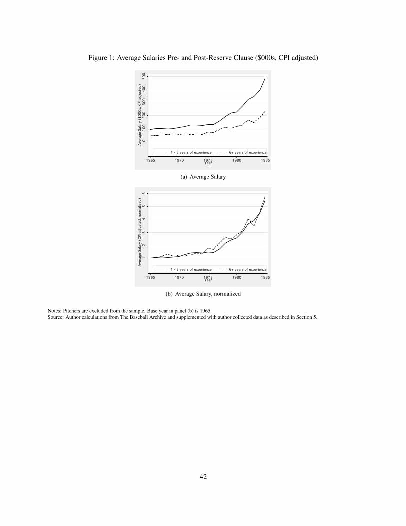
Figure 1: Average Salaries Pre- and Post-Reserve Clause ($000s, CPI adjusted)0

0

0100

100

100200

200

200300

300

300400

400

400500

500

500Average Salary ($000s, CPI adjusted)

Aver

age

Sala

ry (

$000

s, C

PI a

djus

ted)

Average Salary ($000s, CPI adjusted)1965

1965

19651970

1970

19701975

1975

19751980

1980

19801985

1985

1985Year

Year

Year 1 - 5 years of experience

1 - 5 years of experience

1 - 5 years of experience6+ years of experience

6+ years of experience

6+ years of experience

(a) Average Salary1

1

12

2

23

3

34

4

45

5

56

6

6Average Salary (CPI adjusted, normalized)

Aver

age

Sala

ry (

CPI a

djus

ted,

nor

mal

ized

)

Average Salary (CPI adjusted, normalized)1965

1965

19651970

1970

19701975

1975

19751980

1980

19801985

1985

1985Year

Year

Year 1 - 5 years of experience

1 - 5 years of experience

1 - 5 years of experience6+ years of experience

6+ years of experience

6+ years of experience

(b) Average Salary, normalized

Notes: Pitchers are excluded from the sample. Base year in panel (b) is 1965.Source: Author calculations from The Baseball Archive and supplemented with author collected data as described in Section 5.

42

Figure 2: Average Unconditional and Residual Salary by Experience ($000s, CPI adjusted)0

00500

500

500100010

0010001500

1500

1500Average Salary ($000s, CPI adjusted)

Aver

age

Sala

ry (

$000

s, C

PI a

djus

ted)

Average Salary ($000s, CPI adjusted)0

0

05

5

510

10

1015

15

15Experience

Experience

ExperienceMarried

Married

MarriedSingle

Single

SingleAverage Salary by Years of ExperienceAverage Salary by Years of Experience

Average Salary by Years of Experience

(a) Low Ability

-1000

-100

0

-1000-500

-500

-5000

0

0500

500

5001000

1000

10001500

1500

1500Average Residual Salary ($000s, CPI adjusted)

Aver

age

Resid

ual S

alar

y ($

000s

, CPI

adj

uste

d)

Average Residual Salary ($000s, CPI adjusted)0

0

05

5

510

10

1015

15

15Experience

Experience

ExperienceMarried

Married

MarriedSingle

Single

SingleAverage Residual Salary by Years of ExperienceAverage Residual Salary by Years of Experience

Average Residual Salary by Years of Experience

(b) Low Ability0

0

01000

1000

10002000

2000

20003000

3000

30004000

4000

4000Average Salary ($000s, CPI adjusted)

Aver

age

Sala

ry (

$000

s, C

PI a

djus

ted)

Average Salary ($000s, CPI adjusted)0

0

05

5

510

10

1015

15

15Experience

Experience

ExperienceMarried

Married

MarriedSingle

Single

SingleAverage Salary by Years of ExperienceAverage Salary by Years of Experience

Average Salary by Years of Experience

(c) Medium Ability

-1000

-100

0

-1000-500

-500

-5000

0

0500

500

5001000

1000

10001500

1500

1500Average Residual Salary ($000s, CPI adjusted)

Aver

age

Resid

ual S

alar

y ($

000s

, CPI

adj

uste

d)

Average Residual Salary ($000s, CPI adjusted)0

0

05

5

510

10

1015

15

15Experience

Experience

ExperienceMarried

Married

MarriedSingle

Single

SingleAverage Residual Salary by Years of ExperienceAverage Residual Salary by Years of Experience

Average Residual Salary by Years of Experience

(d) Medium Ability0

0

01000

1000

10002000

2000

20003000

3000

30004000

4000

4000Average Salary ($000s, CPI adjusted)

Aver

age

Sala

ry (

$000

s, C

PI a

djus

ted)

Average Salary ($000s, CPI adjusted)0

0

05

5

510

10

1015

15

15Experience

Experience

ExperienceMarried

Married

MarriedSingle

Single

SingleAverage Salary by Years of ExperienceAverage Salary by Years of Experience

Average Salary by Years of Experience

(e) High Ability

-1000

-100

0

-1000-500

-500

-5000

0

0500

500

5001000

1000

10001500

1500

1500Average Residual Salary ($000s, CPI adjusted)

Aver

age

Resid

ual S

alar

y ($

000s

, CPI

adj

uste

d)

Average Residual Salary ($000s, CPI adjusted)0

0

05

5

510

10

1015

15

15Experience

Experience

ExperienceMarried

Married

MarriedSingle

Single

SingleAverage Residual Salary by Years of ExperienceAverage Residual Salary by Years of Experience

Average Residual Salary by Years of Experience

(f) High Ability

Notes: Years 1975 - 2007. Pitchers are excluded from sample.

Source: Author calculations from The Baseball Archive and supplemented with authors collected data as described in Section 5. Low ability single

players are censored at 11 years of experience because beyond this point there are less than 10 total observations.

43

Figure 3: Average Unconditional and Residual Productivity by Experience.65

.65

.65.7.7

.7.75.7

5.75.8

.8.8.85

.85

.85OPS

OPS

OPS0

0

05

5

510

10

1015

15

15Experience

Experience

ExperienceMarried

Married

MarriedSingle

Single

SingleAverage Productivity by Years of ExperienceAverage Productivity by Years of Experience

Average Productivity by Years of Experience

(a) Low Ability

-.04

-.04

-.04-.02

-.02

-.020

0

0.02

.02

.02.04

.04

.04.06

.06

.06Residual OPS

Resid

ual O

PS

Residual OPS0

0

05

5

510

10

1015

15

15Experience

Experience

ExperienceMarried

Married

MarriedSingle

Single

SingleAverage Residual Productivity by Years of ExperienceAverage Residual Productivity by Years of Experience

Average Residual Productivity by Years of Experience

(b) Low Ability.65

.65

.65.7

.7

.7.75

.75

.75.8

.8

.8.85

.85

.85OPS

OPS

OPS0

0

05

5

510

10

1015

15

15Experience

Experience

ExperienceMarried

Married

MarriedSingle

Single

SingleAverage Productivity by Years of ExperienceAverage Productivity by Years of Experience

Average Productivity by Years of Experience

(c) Medium Ability

-.04

-.04

-.04-.02

-.02

-.020

0

0.02

.02

.02.04

.04

.04.06

.06

.06Residual OPS

Resid

ual O

PS

Residual OPS0

0

05

5

510

10

1015

15

15Experience

Experience

ExperienceMarried

Married

MarriedSingle

Single

SingleAverage Residual Productivity by Years of ExperienceAverage Residual Productivity by Years of Experience

Average Residual Productivity by Years of Experience

(d) Medium Ability.65

.65

.65.7

.7

.7.75

.75

.75.8

.8

.8.85

.85

.85OPS

OPS

OPS0

0

05

5

510

10

1015

15

15Experience

Experience

ExperienceMarried

Married

MarriedSingle

Single

SingleAverage Productivity by Years of ExperienceAverage Productivity by Years of Experience

Average Productivity by Years of Experience

(e) High Ability

-.04

-.04

-.04-.02

-.02

-.020

0

0.02

.02

.02.04

.04

.04.06

.06

.06Residual OPS

Resid

ual O

PS

Residual OPS0

0

05

5

510

10

1015

15

15Experience

Experience

ExperienceMarried

Married

MarriedSingle

Single

SingleAverage Residual Productivity by Years of ExperienceAverage Residual Productivity by Years of Experience

Average Residual Productivity by Years of Experience

(f) High Ability

Notes: Years 1975 - 2007. Pitchers are excluded from sample.

Source: Author calculations from The Baseball Archive and supplemented with author collected data as described in Section 5. Low ability single

players are censored at 11 years of experience because beyond this point there are less than 10 total observations.

44

Tabl

e1:

Sum

mar

ySt

atis

tics

Popu

latio

nSa

mpl

e

Var

iabl

eO

bs(p

op/s

ampl

e)M

ean

Std.

Dev

.M

ean

Std.

Dev

.D

escr

iptio

nR

ooki

eYe

arD

emog

raph

ics

age

9,23

6/3,

379

24.1

82.

8424

.19

2.78

age

righ

t8,

578/

3,26

20.

700.

460.

690.

46=1

ifth

epl

ayer

isri

ght-

hand

ed,0

othe

rwis

ele

ft8,

578/

3,26

20.

380.

490.

400.

49=1

ifth

epl

ayer

isle

ft-h

ande

d,0

othe

rwis

ew

hite

NA

/3,3

746

0.80

0.40

=1if

the

play

eris

whi

te,0

othe

rwis

ebl

ack

NA

/3,3

740.

130.

34=1

ifth

epl

ayer

isbl

ack,

0ot

herw

ise

hisp

anic

NA

/3,3

740.

100.

30=1

ifth

epl

ayer

ishi

span

ic,0

othe

rwis

eot

herr

ace

NA

/3,3

740.

010.

07=1

ifot

herr

ace,

0ot

herw

ise

heig

ht7,

782/

2,95

671

.53

2.37

71.6

32.

29H

eigh

tin

inch

esw

eigh

t8,

727/

3,29

518

0.17

24.2

418

1.23

18.2

1W

eigh

tin

poun

ds

Mar

italS

tatu

sand

Wag

es

mar

ried

NA

/19,

294

0.69

0.46

=1if

the

play

eris

mar

ried

,0ot

herw

ise

year

smar

NA

/14,

256

4.30

6.05

=Y

ear-

Yea

rofM

arri

age

wag

esN

A/1

3,71

845

7.43

1036

.66

Yea

rly

Wag

e($

000s

,adj

uste

dfo

rinfl

atio

n)

Prod

uctiv

ityR

elat

edM

easu

res

BA48

,960

/22,

510

0.24

10.

089

0.24

90.

072

Bat

ting

Ave

rage

OB

P46

,770

/21,

787

0.30

70.

096

0.31

60.

079

On-

base

perc

enta

geO

PS

46,7

28/2

1,77

90.

651

0.22

90.

674

0.18

9O

n-ba

sepl

ussl

uggi

ngR

EqA

33,7

15/1

2,41

50.

689

0.22

00.

712

0.17

6E

quiv

alen

tAve

rage

(raw

)W

AR

45,9

61/2

2,05

2.8

461.

792

0.98

61.

877

Win

sA

bove

Rep

lace

men

tG

49,3

56/2

2,57

672

.88

52.2

683

.40

50.0

9N

umbe

rofg

ames

play

edPA

44,7

74/2

1,84

527

0.53

229.

4331

2.26

225.

10Pl

ate

App

eara

nces

Oth

erVa

riab

les

expe

rien

ce49

,357

/22,

576

5.51

4.40

5.72

4.21

Yea

rsin

ML

Bye

ar49

,357

/22,

576

1954

3819

5736

Yea

r(18

71-2

007)

‡

posi

tion

Fiel

ding

posi

tion

team−

ball

park

244

Uni

que

ids

man

ager

513

Uni

que

ids

1.Se

eA

ppen

dix

Afo

rfur

ther

desc

ript

ion

ofth

epr

oduc

tivity

mea

sure

s2.

Fiel

ding

posi

tions

incl

ude

first

base

man

,sec

ond

base

man

,thi

rdba

sem

an,c

atch

er,c

ente

rfiel

d,le

ftfie

ld,r

ight

field

,sho

rtst

op.A

lso

incl

udes

desi

gnat

edhi

ttera

ndou

tfiel

der.

3.A

bout

one

perc

ento

fob

serv

atio

nsar

ein

leag

ues

othe

rth

anA

mer

ican

and

Nat

iona

l,th

ese

are

prim

arily

from

the

earl

yda

ysof

base

ball

and

disa

ppea

red

byth

eea

rly

1900

s.T

hey

are

incl

uded

alon

gw

ithth

eN

atio

nalL

eagu

ein

alle

stim

atio

nm

odel

s.

4.W

age

equa

tions

are

limite

dto

1905

-200

7du

eto

data

avai

labi

lity.

45

Table 2: The Effect of Marital Status on Log Earnings (The “Marriage Premium")

Pre-1975 Post-1975OLS FE OLS FE OLS FE OLS FE(1) (2) (3) (4) (5) (6) (7) (8)

marriedy−1 .025 -.008 -.007 .035(.025) (.026) (.033) (.050)

marriedy−1×ability1 .012 -.034 -.002 -.101(.040) (.061) (.059) (.110)

marriedy−1×ability2 .027 .017 -.128 -.137(.037) (.039) (.053)∗∗ (.099)

marriedy−1×ability3 .028 -.014 .053 .160(.033) (.036) (.046) (.061)∗∗∗

ability1 6.244 10.309(.682)∗∗∗ (1.313)∗∗∗

ability2 6.212 10.427(.680)∗∗∗ (1.314)∗∗∗

ability3 6.295 10.453(.680)∗∗∗ (1.313)∗∗∗

cons 4.972 -4.312 -4.323 10.172 32.132 31.521(.589)∗∗∗ (1.161)∗∗∗ (1.156)∗∗∗ (1.228)∗∗∗ (2.540)∗∗∗ (2.554)∗∗∗

Obs. 4401 4401 4401 4401 6442 6442 6442 6442R2 .868 .947 .838 .947 .811 .89 .814 .890

Dependent variable is equal to log(salary)y. Robust standard errors, clustered on player id in parentheses. All models controlfor team-ballpark, position, manager, and year effects. OLS controls include: age and its square, experience and its square, racedummies, height, weight, left/right handed, lagged games played, and indicators for more than three and more than six yearsof experience. FE controls include: age and experience squared, lagged games played, and indicators for more than three andmore than six years of experience.Columns 3 and 7 are estimated without a constant. R2 in these models are obtained from the equivalent model estimated with aconstant.∗10 percent significance level, ∗∗5 percent significance level, ∗∗∗1 percent significance level.

46

Table 3: The Effect of Marital Status on Productivity

Pre-1975 Post-1975OLS FE OLS FE OLS FE OLS FE(1) (2) (3) (4) (5) (6) (7) (8)

Panel A: BA

marriedy−1 .002 -.000 -.001 .002(.002) (.002) (.001) (.002)

marriedy−1×ability1 .001 -.007 .005 .007(.004) (.007) (.003)∗ (.004)∗

marriedy−1×ability2 .004 -.000 -.003 -.001(.003) (.004) (.002) (.004)

marriedy−1×ability3 .002 .001 -.001 .001(.002) (.002) (.002) (.002)

ability1 .162 .298(.056)∗∗∗ (.054)∗∗∗

ability2 .157 .304(.056)∗∗∗ (.054)∗∗

ability3 .161 .306(.056)∗∗∗ (.054)∗∗∗

cons .161 .057 .058 .316 .569 .572(.055)∗∗∗ (.066) (.066) (.054)∗∗∗ (.097)∗∗∗ (.096)∗∗∗

Obs 5660 5660 5660 5660 5844 5844 5844 5844R2 .394 .646 .352 .646 .192 .506 .195 .507

Panel B: OPS

marriedy−1 .003 -.001 -.006 .004(.005) (.006) (.005) (.005)

marriedy−1×ability1 .000 -.016 .006 .011(.012) (.023) (.008) (.011)

marriedy−1×ability2 .007 .001 -.012 -.005(.008) (.011) (.008) (.011)

marriedy−1×ability3 .0009 -.001 -.009 .005(.006) (.007) (.006) (.006)

ability1 1.154 .411(.127)∗∗∗ (.163)∗∗∗

ability2 1.134 .426(.126)∗∗∗ (.163)∗∗∗

ability3 1.151 .436(.127)∗∗∗ (.162)∗∗∗

cons 1.006 -.196 -.199 .492 1.937 1.931(.133)∗∗∗ (.183) (.184) (.164)∗∗∗ (.334)∗∗∗ (.331)∗∗∗

Obs 5593 5593 5593 5593 5844 5844 5844 5844R2 .432 .713 .391 .714 .361 .632 .365 .633

Dependent variable is equal to productivity (BA, OPS). Robust standard errors, clustered on player id in parentheses. All modelscontrol for team-ballpark, position, manager, and year fixed effects. OLS controls include: age and its square, experience andits square, race dummies, height, weight, left/right handed, lagged games played, and indicators for more than three and morethan six years of experience. FE controls include: age and experience squared, lagged games played, and indicators for morethan three and more than six years of experience. Sample restricted to observations with at least 100 plate appearances.∗10 percent significance level, ∗∗5 percent significance level, ∗∗∗1 percent significance level.

47

Table 4: The Direct Effect of Marriage on Earnings (Controling for Productivity)

Pre-1975 Post-1975OLS FE OLS FE OLS FE OLS FE(1) (2) (3) (4) (5) (6) (7) (8)

marriedy−1 .017 -.0002 .019 .082(.023) (.023) (.032) (.051)

marriedy−1×ability1 .026 .037 .071 .024(.041) (.060) (.069) (.126)

marriedy−1×ability2 .002 .008 -.112 -.078(.037) (.041) (.054)∗∗ (.110)

marriedy−1×ability3 .022 -.008 .059 .160(.031) (.029) (.042) (.059)∗∗∗

ability1 4.553 8.875(.684)∗∗∗ (1.157)∗∗∗

ability2 4.554 9.072(.676)∗∗∗ (1.159)∗∗∗

ability3 4.637 9.102(.677)∗∗∗ (1.155)∗∗∗

OPSy−1 1.463 .868 1.462 .867 2.107 1.004 2.026 1.002(.098)∗∗∗ (.077)∗∗∗ (.098)∗∗∗ (.077)∗∗∗ (.123)∗∗∗ (.134)∗∗∗ (.121)∗∗∗ (.133)∗∗∗

cons 3.585 -5.198 -4.827 9.508 30.051 29.631(.651)∗∗∗ (1.025)∗∗∗ (1.070)∗∗∗ (1.358)∗∗∗ (2.652)∗∗∗ (2.681)∗∗∗

Obs 3662 3662 3662 3662 5390 5390 5390 5390R2 .894 .960 .862 .960 .821 .894 .825 .895

Dependent variable is equal to log(salary)y. Robust standard errors, clustered on player id in parentheses. All models control for team-ballpark,position, manager, and year effects. OLS controls include: age and its square, experience and its square, race dummies, height, weight, left/righthanded, lagged games played, and indicators for more than three and more than six years of experience. FE controls include: age and experiencesquared, lagged games played, and indicators for more than three and more than six years of experience. Sample restricted to observations withat least 100 plate appearances. See Table 9 for expanded results.∗10 percent significance level, ∗∗5 percent significance level, ∗∗∗1 percent significance level.

48

Table 5: Endogenous Attrition: Robustness Tests

Exper.≤ 4yrs Exper.≤ 8yrs Exper.≤ 12yrs Exper.≤ 16yrs Exper.≤ 20yrs IPW(1) (2) (3) (4) (5) (6)

Panel A: OLS

marriedy−1×ability1 .034 .113 .076 .078 .070 .057(.110) (.084) (.074) (.067) (.069) (.062)

marriedy−1×ability2 -.026 -.067 -.123 -.124 -.115 -.092(.072) (.061) (.060)∗∗ (.055)∗∗ (.054)∗∗ (.047)∗∗

marriedy−1×ability3 .139 .087 .044 .048 .056 .087(.060)∗∗ (.048)∗ (.046) (.043) (.042) (.047)∗

ability1 15.222 9.447 6.518 7.916 8.894 7.732(2.456)∗∗∗ (1.833)∗∗∗ (1.473)∗∗∗ (1.400)∗∗∗ (1.317)∗∗∗ (1.295)∗∗∗

ability2 15.352 9.654 6.711 8.121 9.065 7.886(2.447)∗∗∗ (1.833)∗∗∗ (1.477)∗∗∗ (1.400)∗∗∗ (1.315)∗∗∗ (1.294)∗∗∗

ability3 15.481 9.751 6.783 8.158 9.129 7.913(2.440)∗∗∗ (1.824)∗∗∗ (1.469)∗∗∗ (1.396)∗∗∗ (1.313)∗∗∗ (1.293)∗∗∗

OPSy−1 1.364 1.965 1.945 2.005 2.037 2.122(.179)∗∗∗ (.152)∗∗∗ (.134)∗∗∗ (.124)∗∗∗ (.121)∗∗∗ (.139)∗∗∗

R2 .796 .833 .835 .829 .827 .806Panel B: FE

marriedy−1×ability1 .078 .139 .142 .037 .021 -.014(.353) (.141) (.124) (.111) (.125) (.137)

marriedy−1×ability2 -.003 -.089 -.164 -.140 -.091 -.026(.295) (.119) (.131) (.110) (.111) (.118)

marriedy−1×ability3 .028 .175 .141 .141 .157 .169(.144) (.065)∗∗∗ (.061)∗∗ (.061)∗∗ (.059)∗∗∗ (.064)∗∗∗

OPSy−1 1.021 1.156 .972 .900 .986 .994(.383)∗∗∗ (.157)∗∗∗ (.137)∗∗∗ (.126)∗∗∗ (.134)∗∗∗ (.146)∗∗∗

cons 43.494 44.609 39.902 34.138 30.782 28.947(23.297)∗ (4.049)∗∗∗ (2.954)∗∗∗ (3.020)∗∗∗ (3.009)∗∗∗ (3.213)∗∗∗

R2 .968 .938 .921 .901 .896 .892

Obs 1344 2979 4148 5212 5362 5238

Dependent variable is equal to log(salary)y. Robust standard errors, clustered on player id in parentheses. All models control for team-ballpark, position, manager, and year effects. OLS controls include: age and its square, experience and its square, race dummies, height,weight, left/right handed, lagged games played, and indicators for more than three and more than six years of experience. FE controlsinclude: age and experience squared, lagged games played, and indicators for more than three and more than six years of experience.OLS models are estimated without a constant. R2 in these models are obtained from the equivalent model estimated with a constant.Sample restricted to observations with at least 100 plate appearances.∗10 percent significance level, ∗∗5 percent significance level, ∗∗∗1 percent significance level.

49

Table 6: The Effect of Earnings on Future Marital Status (Test of Reverse Causality)

OLS OLS OLS OLS(1) (2) (3) (4)

experience3yrs+ .026(.025)

experience6yrs+ -.005(.037)

log(salary)y−1 -.006(.015)

∆log(salary)y−1 .024(.030)

∆log(OPS)y−1 -.061(.057)

cons -.088 -1.063 -1.076 -1.689(.819) (.940) (1.438) (1.308)

Obs. 2170 1718 1213 1281R2 .152 .180 .235 .217

Dependent variable is equal to one if year of marriage occurs in year y + 1, zero otherwise. All models control for team-ballpark, position, manager, and year effects and are estimated by OLS with robust standard errors, clustered on player id inparentheses. OLS controls include: age and its square, experience and its square, race dummies, height, weight, left/righthanded, and lagged games played.∗10 percent significance level, ∗∗5 percent significance level, ∗∗∗1 percent significance level.

50

Table 7: The Effect of Marital Status on Performance Stability and Wage Underpayment

OLS FE OLS OLS OLS OLS(1) (2) (3) (4) (5) (6)

marriedy−1×ability1 -.050 -.061 .766 .984 .061 .120(.016)∗∗∗ (.025)∗∗ (3.557) (3.565) (.107) (.105)

marriedy−1×ability2 -.014 .008 2.923 3.039 .135 .136(.015) (.021) (2.658) (2.665) (.095) (.095)

marriedy−1×ability3 .010 .027 -4.816 -4.377 -.074 -.049(.009) (.010)∗∗∗ (1.789)∗∗∗ (1.884)∗∗ (.043)∗ (.044)

ability1 .032 46.285 105.297 2.392 1.641(.186) (26.514)∗ (49.751)∗∗ (.770)∗∗∗ (2.002)

ability2 -.020 44.613 103.507 2.269 1.549(.187) (26.332)∗ (49.542)∗∗ (.768)∗∗∗ (1.985)

ability3 -.046 49.642 108.311 2.349 1.619(.185) (25.992)∗ (49.087)∗∗ (.761)∗∗∗ (1.987)

cons .009(.327)

Obs 6413 6413 647 647 647 647R2 .272 .568 .419 .555 .264 .555

Columns 1 - 2: Dependent variable is equal to the coefficient of variance of OPS as described in the text. Columns 3 - 4: Dependent variableis equal to exploitation/100,000 (marginal revenue product minus salary). Columns 5 - 6: Dependent variable is equal to exploitation/MRP.Robust standard errors, clustered on player id in parentheses. Columns 1 - 2 control for team-ballpark, position, manager, and year effects.Columns 3 - 6 control for team-ballpark, position and year effects. OLS (columns 1,4,6) controls include: age and its square, experience andits square, race dummies, height, weight, left/right handed, lagged games played, and indicators for more than three and more than six yearsof experience. OLS (columns 3,5) controls include: age, experience, race dummies, height, weight, left/right handed, lagged games played,and indicators for more than three and more than six years of experience. FE (column 2) controls include: age and experience squared, laggedgames played, and indicators for more than three and more than six years of experience. OLS models are estimated without a constant. R2 inthese models are obtained from the equivalent model estimated with a constant.∗10 percent significance level, ∗∗5 percent significance level, ∗∗∗1 percent significance level.

51

Table 8: The Effect of Marital Status on Ballpark Attendance and Team Wins

OLS FE OLS FE(1) (2) (3) (4)

married .172 .175 .026 .020(.073)∗∗ (.082)∗∗ (.011)∗∗ (.012)∗

home 4.089 3.508 .345 .257(.963)∗∗∗ (.744)∗∗∗ (.112)∗∗∗ (.115)∗∗

worldseriesy−1 .047 .056(.028)∗ (.025)∗∗

winsy−1 1.605 1.160(.160)∗∗∗ (.145)∗∗∗

BA 3.736 3.624(.125)∗∗∗ (.142)∗∗∗

ERA -.108 -.107(.002)∗∗∗ (.003)∗∗∗

cons 9.109 12.176 -.254 -.228(.494)∗∗∗ (.465)∗∗∗ (.062)∗∗∗ (.073)∗∗∗

Obs 1929 1929 2135 2135R2 .892 .934 .826 .854

The dependent variable in columns 1 - 2 is equal to the log of ballpark attendance, in columns 3 - 4 it is the number of wins divided by gamesplayed (wins). The variable married is the team level fraction of married players. home is the fraction of homegames divided by total games.worldseries is a binary indicator equal to one if the team was in the world series. BA is the team level batting average over all batters. ERA isthe team level earned runs average over all pitchers. Robust standard errors, in parentheses, are clustered by team-ballpark. All columns controlfor year and manager effects.∗10 percent significance level, ∗∗5 percent significance level, ∗∗∗1 percent significance level.

52

12 Appendix

A Glossary of Terms

1. AB (at-bats): Batting appearances, not including bases on balls, hit by pitch, sacrifices, interference,

or obstruction.

2. All-Star: The Major League Baseball All-Star Game is an annual exhibition baseball game between

the best players from the National League and the American League.

3. BA (batting average): The ratio of hits (H) to at bats (AB).

4. BB (base on balls): A base on balls (BB) is credited to a batter and against a pitcher in baseball

statistics when a batter receives four pitches that the umpire calls balls.

5. ERA (earned run average): Is the mean of earned runs given up by a pitcher per nine innings pitched.

It is determined by dividing the number of earned runs allowed by the number of innings pitched and

multiplying by nine.

6. H (hits): A hit, also called a base hit, is credited to a batter when the batter safely reaches first base

after hitting the ball into fair territory, without the benefit of an error or a fielder’s choice.

7. HBP (hit by pitch): Is a batter or his equipment (other than his bat) being hit in some part of his body

by a pitch from the pitcher.

8. OBP (on base percentage): Is a measure of how often a batter reaches base for any reason other

than a fielding error, fielder’s choice, dropped/uncaught third strike, fielder’s obstruction, or catcher’s

interference. Is determinard by the following formula: (H + BB + HBP)/(AB + BB + HBP + SF).

9. OPS (on base plus slugging): OBP plus slugging average.

10. PA (plate appearances): At bats (AB) + some of the scenarios excluded from at bats such as base on

balls (BB), hit by pitch (HBP), sacrifice (SF) + times reached on defensive interference.

53

11. SF (sacrifice fly): Is a batted ball that satisfies four criteria: 1. There are fewer than two outs when

the ball is hit; 2. The ball is hit to the outfield; 3. The batter is out because an outfielder or an infielder

running in the outfield catches the ball (or would have been out if not for an error); 4. A runner who

is already on base scores on the play.

12. SH (sacrifice hit): Is the act of deliberately bunting the ball in a manner that allows a runner on base

to advance to another base.

13. Slugging percentage: Is a popular measure of the power of a hitter. It is calculated as total bases

divided by at-bats.

14. REqA (equivalent average): Is a metric intended to express the production of hitters in a context

independent of park and league effects. It is give by the following formula: (H + TB + 1.5(BB+HBP)

+ SB + SH + SF)/(AB + BB +HBP +SH + SF + CS + SB/3).

15. T B (total bases): The number of bases a player has gained with hits, i.e., the sum of his hits weighted

by 1 for a single, 2 for a double, 3 for a triple and 4 for a home run. Only bases attained from hits

count toward this total.

16. WAR (Wins Above Replacement): The number of wins a player provides the team above what a team

would win were it to replace the player with an average minor league player off the bench.

B Table 4 Expanded Results

54

Table 9: The Direct Effect of Marriage on Earnings by Initial Ability (Controlling for Productivity)

Pre-1975 Post-1975OLS FE OLS FE OLS FE OLS FE(1) (2) (3) (4) (5) (6) (7) (8)

marriedy−1 .017 -.0002 .019 .082(.023) (.023) (.032) (.051)

marriedy−1×ability1 .026 .037 .071 .024(.041) (.060) (.069) (.126)

marriedy−1×ability2 .002 .008 -.112 -.078(.037) (.041) (.054)∗∗ (.110)

marriedy−1×ability3 .022 -.008 .059 .160(.031) (.029) (.042) (.059)∗∗∗

ability1 -.016 -.197(.048) (.073)∗∗∗

ability2

ability3 .078 .030(.039)∗∗ (.055)

OPSy−1 1.463 .868 1.462 .867 2.107 1.004 2.026 1.002(.098)∗∗∗ (.077)∗∗∗ (.098)∗∗∗ (.077)∗∗∗ (.123)∗∗∗ (.134)∗∗∗ (.121)∗∗∗ (.133)∗∗∗

age .141 .143 .028 .028(.030)∗∗∗ (.031)∗∗∗ (.063) (.062)

age2 -.002 -.004 -.002 -.004 -.001 -.008 -.001 -.008(.0005)∗∗∗ (.0006)∗∗∗ (.0005)∗∗∗ (.0006)∗∗∗ (.001) (.002)∗∗∗ (.001) (.002)∗∗∗

experience .124 .125 .276 .279(.013)∗∗∗ (.013)∗∗∗ (.029)∗∗∗ (.029)∗∗∗

experience2 -.003 -.002 -.003 -.002 -.008 -.004 -.008 -.005(.0007)∗∗∗ (.0006)∗∗∗ (.0007)∗∗∗ (.0006)∗∗∗ (.001)∗∗∗ (.002)∗∗ (.001)∗∗∗ (.002)∗∗∗

Gy−1 .004 .002 .004 .002 .008 .004 .008 .005(.0002)∗∗∗ (.0002)∗∗∗ (.0002)∗∗∗ (.0002)∗∗∗ (.0004)∗∗∗ (.0004)∗∗∗ (.0004)∗∗∗ (.0004)∗∗∗

le f t .080 .091 .027 .018(.053) (.048)∗ (.045) (.045)

right .145 .155 -.002 -.004(.055)∗∗∗ (.049)∗∗∗ (.050) (.050)

black .197 .194 .046 .084(.055)∗∗∗ (.056)∗∗∗ (.065) (.066)

white .177 .173 .021 .056(.063)∗∗∗ (.064)∗∗∗ (.067) (.067)

hispanic .100 .096 -.002 .019(.059)∗ (.061) (.057) (.058)

other race .467 .458(.386) (.370)

height -.006 -.006 .008 .014(.007) (.007) (.010) (.010)

weight .001 .001 .003 .002(.001) (.0009) (.001)∗∗ (.001)

experience3yrs+ -.0008 .079 .010 .079 .360 .480 .373 .475(.021) (.019)∗∗∗ (.021) (.019)∗∗∗ (.047)∗∗∗ (.050)∗∗∗ (.047)∗∗∗ (.050)∗∗∗

experience6yrs+ .025 .039 .022 .039 .183 .210 .180 .213(.018) (.017)∗∗ (.018) (.017)∗∗ (.040)∗∗∗ (.042)∗∗∗ (.040)∗∗∗ (.042)∗∗∗

cons 3.585 -5.198 -4.827 9.508 30.051 29.631(.651)∗∗∗ (1.025)∗∗∗ (1.070)∗∗∗ (1.358)∗∗∗ (2.652)∗∗∗ (2.681)∗∗∗

Obs 3662 3662 3662 3662 5390 5390 5390 5390R2 .894 .960 .862 .960 .821 .894 .825 .895

Dependent variable is equal to log(salary)y. Robust standard errors, clustered on player id in parentheses. All models controlfor team-ballpark, position, manager, and year effects. OLS controls include: age and its square, experience and its square, racedummies, height, weight, left/right handed, lagged games played, and indicators for more than three and more than six years ofexperience. FE controls include: age and experience squared, lagged games played, and indicators for more than three and morethan six years of experience. OLS models are estimated without a constant. R2 in these models are obtained from the equivalentmodel estimated with a constant. Sample restricted to observations with at least 100 plate appearances.∗10 percent significance level, ∗∗5 percent significance level, ∗∗∗1 percent significance level.

55