Productivity Growth of East Asia Economies’ Manufacturing:

A Decomposition Analysis

Hailin Liao*, Mark Holmes,

Tom Weyman-Jones, David Llewellyn

Loughborough University

Abstract Applying a stochastic production frontier to sector-level data within manufacturing, this paper examines total factor productivity (TFP) growth for eight East Asian economies during 1963-1998, using both single country and cross-country regression. The analysis focuses on the trend of technological progress (TP) and technical efficiency change (TEC), and the role of productivity change in economic growth. The empirical results reveal that although input factor accumulation is still the main source for East Asian economies’ growth, TFP growth is accounting for an increasing and important proportion of output growth, among which the improved TEC plays a crucial role in productivity growth. Key Words: total factor productivity; technical efficiency change; technological progress; stochastic production frontier; East Asian Economy JEL Classification Numbers: D24, L60, O30, O53, O47 (7987 words, submitted on 19th December 2002)

* Corresponding author, e-mail: h.liao@lboro.ac.uk

1

Productivity Growth of East Asia Economies’ Manufacturing:

A Decomposition Analysis

1. Introduction The East Asia economic ‘miracle’ and the subsequent recessions following the Asian financial crisis in 1997 have received great attention from economists. One debate has concentrated on decomposing output growth into factor accumulation and productivity gains, to see whether the impressive growth can be sustained. Accumulationists believe that the increased use and accumulation of inputs (especially the investment) rather than the increases in productivity explain all growth, Young (1992, 1994a, 1994b, 1995), Krugman (1994), Collins & Bosworth (1996), Drysdale & Huang (1997), Crafts (1999a, 1999b); assimilationists are persuaded that answer to growth lies in the use of more efficient technology, World Bank (1993), Sarel (1996, 1997), Nelson & Pack (1999). In the above studies, there is an implicit assumption that the economies are producing along the production possibility frontier with full technical efficiency. Except for Kim & Lau (1994) and Chang & Luh (1999), these studies adopted the conventional growth accounting approach and estimated total factor productivity (TFP) growth without distinguishing between its two components: technical progress (TP) and technical efficiency change (TEC); rather TP is synonymously considered to be the unique source of TFP growth. Defined this way, TFP growth is at best a measure of Hicks-neutral disembodied technological change and at worst nothing more than ‘a measure of our ignorance’ (Abramovitz, 1956; Hulten, 2000). More important, failure to take account of inefficiency and TEC may produce misleading and biased TFP estimates: while high rates of TP can coexist with deteriorating technical efficiency, relatively low rates of TP can also coexist with improving technical efficiency (Nishimizu & Page, 1982); and different policy implications result from different sources of variation in TFP. The stochastic frontier production function approach, applied in this paper, allows us to separate out these two components, and to identify productivity growth due to either improvement in efficiency or progress in technology. The original technique was popularized by Nishimizu & Page (1982). More recent empirical work includes Fare, Grosskopf, Norris & Zhang (1994), who employed a nonparametric approach; Leung (1998), who also estimated Malmquist Index for Singapore’s manufacturing sectors; Wu (2000), who presents an economy-level study on China using an econometric model. Most studies are restricted to comparisons of total economy growth and their sources by using aggregate economy-level data, and diverging trends at a more disaggregated level are ignored. This paper differs from the earlier literature in its specific focus on the measurement within manufacturing sector level since manufacturing is the prominent factor in a country’s process of industrialization and modernization. Moreover, the translog production function, as used in this study, is more appropriate to describe production activities at the firm or industry level, rather than aggregate country level. The objective of this paper is to apply a stochastic frontier production model to identify the sources of economic growth in eight East Asian economies from 1963 - 1998. This study also enables us to examine industry-level TFP performance by using sector-level data, which may help uncover the specificities of growth performance. Section 2 outlines the stochastic frontier production function methodology employed to measure rates of TFP growth. Section 3 describes the data issues, and the empirical results and discussion are presented in Section 4 and 5. The final section contains the conclusions.

2

2. Methodology

2.1 Decomposition of TFP The most important difference between the frontier approach and the traditional index number approach to productivity growth analysis lies in one assumption: the existence of an unobservable and idealized production possibility frontier with production-unit specific one-sided deviation from the frontier, i.e. explicitly allow for the inefficiency. If a production unit operates beneath the production frontier, then its distance from the maximal measures its technical inefficiency (Farrell, 1957; Lovell, 1993; Kumbhakar & Kovell, 2000). Put differently, the frontier approach is capable of capturing both efficiency change and technological change as components of productivity change, which introduces an additional dimension to the analysis from the policy perspective. (Nishimizu & Page, 1982; Bayarsaihan, Battese & Coelli, 1998). We define this so called ‘best practice’ function f(.) as,

),( txfy itFit = (1)

where is the potential output level on the frontier at time t for production unit i, given technology f(.), and is a vector of inputs. Take logs and totally differentiate (1) with respect to time to get

Fity

itx

dtdx

xtxf

ttxf

dttxfd

y jt

jt

it

j

ititF

it ∂∂

+∂

∂== ∑

• ),(ln),(ln),(ln

∑+=j

jtjt dt

dxTP ε (2)

where the first term on the right-hand side is the output elasticity of frontier output with respect to time, defined as TP, the second term measures the input growth weighted by output elasticities with respect to input

j, jt

itjt x

xf∂

∂=

)(lnε . Note that, the conventional conceptualization of TFP growth can be defined as output

growth unexplained by input growth1, i.e.

∑−≡••

j

jtjt

F

it dtdx

yTFP ε (3)

combining equation (2) and (3), one can get

TPt

txfdt

dxyTFP it

j

jtjt

F

it =∂

∂=−≡ ∑

•• ),(lnε (4)

that is, TP is the only source of TFP growth. Following Nishimizu & Page (1982), a stochastic element can be introduced in the production function. Then, any observed output using for inputs can be expressed as, ity itx

)exp(),()exp( itititititFitit vutxfvuyy +−=+−= (5)

where is a composed error term combining output-based technical inefficiency u , and a symmetric component capturing random variation across production unit and random shocks that are external to its control. The derivative of the logarithm of (5) with respect to time is given by

)( itit vu +− it

itv

dtdu

dtdx

TPdt

dvdt

dudt

txfdy itjt

jtj

itititit −+=+−= ∑

•

ε),(ln

(6)

1 Here the output elasticities with respect to input j is equal to input share in the total production cost under the assumption of perfect competition, due to the lack of data on input price.

3

From equation (6), TFP growth consists of two components: technical change (innovation and shifts in the frontier technology) and technical efficiency change (catching-up), that is,

dtdu

TPTFP it−=•

(7)

This decomposition of TFP growth is useful in distinguishing innovation or adoption of new technology by ‘best practice’ production units from the diffusion of technology. Coexistence of a high rate of TP and a low rate of change in technical efficiency may reflect the failures in achieving technological mastery or diffusion (Kalirajan, Obwona & Zhao, 1996). Nishimizu & Page (1982, p926) ignored the presence of measurement error ( v ) in estimating the parameters of this translog approximation to equation (5) by using a deterministic frontier. In this study, we are going to estimate equation (5) allowing for v with an attempt to distinguish the effects of statistical noise from those of inefficiency so as to obtain consistent and efficient estimates.

it

it

2.2 Model Specification In our empirical analysis, we opt for a parametric approach by considering the time-varying stochastic production frontier, originally proposed by Aigner, Lovell & Schmidt (1977) and Meeusen & van den Broeck (1977)2, in translog form3 as

∑∑ ∑∑ −++++++=j l

ititj

jittjttjitlitjltjitj

jit uvxttxxtxy ln21lnln

21lnln 2

0 βββααα (8)

rather than pursuing a mathematical programming approach, such as DEA Malmquist Index which is deterministic in nature (as do Fare et al. 1985; Fare et al 1994; Leung, 1998; etc). It is easy to debate the relative merits of this way, including the grounding in economic theory, the flexibility of translog from, less sensitive to extreme observations and measurement error or other statistical noise in the data due to modeled distributions of errors and efficiency, and so on (Sharma, Leung & Zaleski, 1997). For the case of agricultural and manufacturing application in developing countries, stochastic frontier analysis are likely to be more appropriate than DEA where the data are heavily influenced by measurement error. In equation (8), is the observed output, t is the time variable and x variables are inputs, subscripts j and l index inputs. The efficiency error, u, accounting for production loss due to unit-specific technical inefficiency, is always greater than or equal to zero and assumed to be independent of the random error, v, which is assumed to have the usual properties (~iid N(0, )). Equation (8) can be rewritten as the following form,

ity

2vσ

))(ln(ln)(ln21)(ln

21lnlnln 22

0 iiLKiKKiLLiKiLit KLKLKLy βββααα +++++=

)(21)(ln)(ln 2

ititttttitKitL uvtttKtL −+++++ βαββ (9)

where is the value-addedity 4.

The above specification allows the estimation of both TP in the stochastic frontier and time-varying technical efficiency. Note that the translog parameterization of this stochastic frontier model allows for non-neutral TP. TP is neutral if all tjβ s are equal to zero. The production function reduces to the Cobb-Douglas function with

neutral TP if all the β s are equal to zero.

2 The original stochastic production frontier with component error, only applied to cross-section analysis, is motivated to deal with panel data by Battese & Coelli (1992, 1995), and further included time trend as a proxy for the disembodied technical change. See Kumbhakar & Lovell (2000, p285-6) for detailed explanation. 3 Diewert (1976) provides a theoretical foundation for using the translog index in productivity analysis. 4 See Schreyer (2001), Kim (2000) and Jorgenson et al. (1987, p242) for the discussion of their use of value-added.

4

The distribution of technical inefficiency effects, u , is taken to be the non-negative truncation of the normal

distribution N(µ, ), modeled, following Battese & Coelli (1992, Greene 1997, p119), to be the product of an exponential function of time as

it2uσ

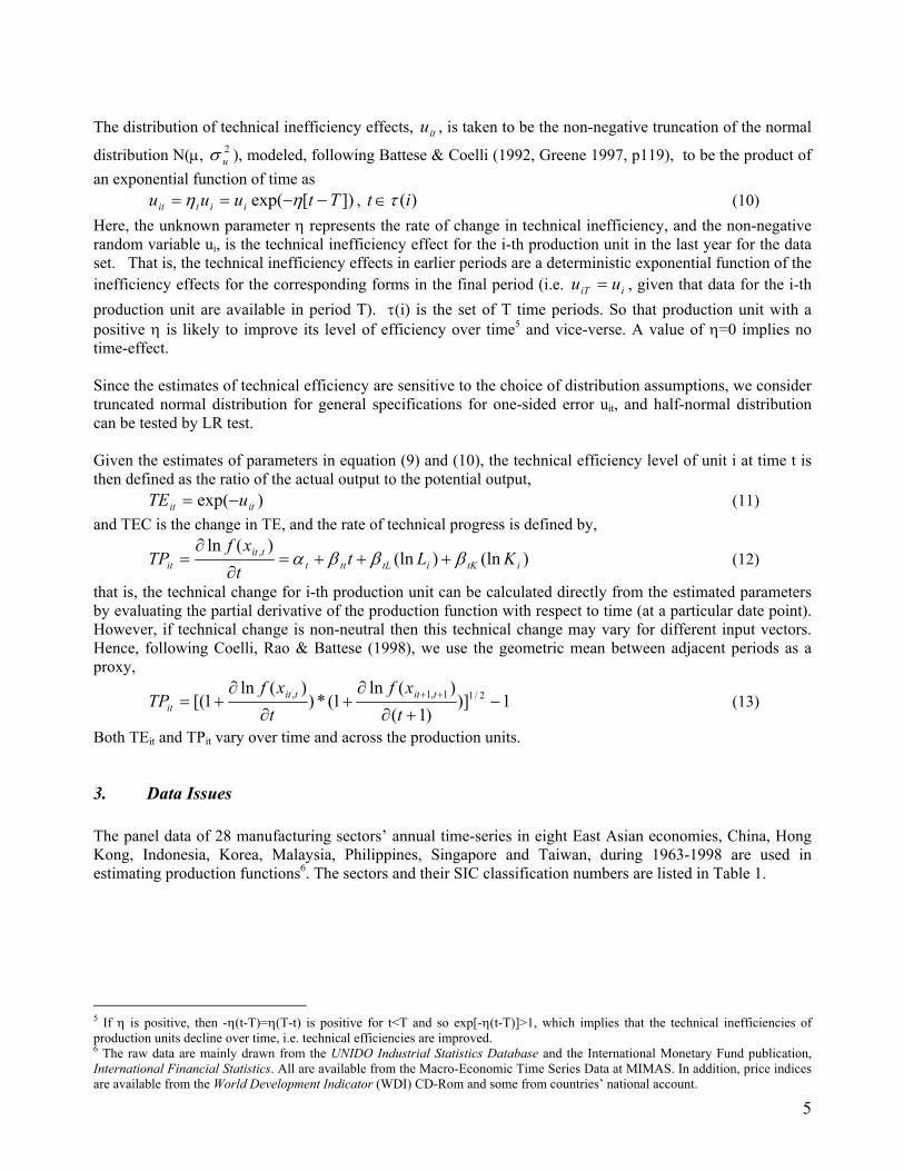
])[exp( Ttuuu iitit −−== ηη , )(it τ∈ (10) Here, the unknown parameter η represents the rate of change in technical inefficiency, and the non-negative random variable ui, is the technical inefficiency effect for the i-th production unit in the last year for the data set. That is, the technical inefficiency effects in earlier periods are a deterministic exponential function of the inefficiency effects for the corresponding forms in the final period (i.e. iiT uu = , given that data for the i-th production unit are available in period T). τ(i) is the set of T time periods. So that production unit with a positive η is likely to improve its level of efficiency over time5 and vice-verse. A value of η=0 implies no time-effect. Since the estimates of technical efficiency are sensitive to the choice of distribution assumptions, we consider truncated normal distribution for general specifications for one-sided error uit, and half-normal distribution can be tested by LR test. Given the estimates of parameters in equation (9) and (10), the technical efficiency level of unit i at time t is then defined as the ratio of the actual output to the potential output, (11) )exp( itit uTE −=and TEC is the change in TE, and the rate of technical progress is defined by,

)(ln)(ln)(ln ,

itKitLttttit

it KLttxf

TP βββα +++=∂

∂= (12)

that is, the technical change for i-th production unit can be calculated directly from the estimated parameters by evaluating the partial derivative of the production function with respect to time (at a particular date point). However, if technical change is non-neutral then this technical change may vary for different input vectors. Hence, following Coelli, Rao & Battese (1998), we use the geometric mean between adjacent periods as a proxy,

1)])1(

)(ln1(*)

)(ln1[( 2/11,1, −

+∂

∂+

∂

∂+= ++

txf

txf

TP tittitit (13)

Both TEit and TPit vary over time and across the production units.

3. Data Issues The panel data of 28 manufacturing sectors’ annual time-series in eight East Asian economies, China, Hong Kong, Indonesia, Korea, Malaysia, Philippines, Singapore and Taiwan, during 1963-1998 are used in estimating production functions6. The sectors and their SIC classification numbers are listed in Table 1.

5 If η is positive, then -η(t-T)=η(T-t) is positive for t<T and so exp[-η(t-T)]>1, which implies that the technical inefficiencies of production units decline over time, i.e. technical efficiencies are improved. 6 The raw data are mainly drawn from the UNIDO Industrial Statistics Database and the International Monetary Fund publication, International Financial Statistics. All are available from the Macro-Economic Time Series Data at MIMAS. In addition, price indices are available from the World Development Indicator (WDI) CD-Rom and some from countries’ national account.

5

Table 1 Manufacturing Sectors 311-Food Products 342-Printing & Publishing 371-Iron & Steel 313-Beverages 351-Industrial Chemicals 372-Non-ferrous Metal 314-Tobacco 352-Other chemical 381-Fabricated Metal Products 321-Textiles 353-Petroleum refineries 382-Machinery, except Electric 322-Wearing Apparel 354-Misc. Petroleum & Coal 383-Machinery, Electric 323-Leather Products 355-Rubber Products 384-Transport Equipment 324-Footwear 356-Plastic Products 385-Professional & Scientific Equipment 331-Wood Products 361-Pottery, China, Earthenware 390-Other Manufactured Products 332-Furniture 362-Glass and Products 341-Paper & Products 369-Other Non-metallic Mineral For single country panels, the number of industrial sectors depends on data availability for each country individually. One problem in cross country regression is that many countries report data for combinations of one or more ISIC groups, for example, Taiwan has only 12 combined sectors, and we consequently had to exclude either the countries or industries in question from the analysis. Because of such difference, we decided to merge some subgroups into one industry, with the goal of capturing sectors that are likely to have more similar technologies as well. In addition, some industries are excluded from the analysis for the reason that these sectors are lacking for many countries. These left us with 12 industry sectors, which have no missing data for all the eight countries, for cross-country regression. Table 2 Cross-country Comparison in Matched Manufacturing Sectors Categories No. Combination of Manufacturing Sectors 0 Total Manufacturing Traditional 1 311/3/4-Food , Beverages & Tobacco Products Traditional 2 321-Textiles Traditional 3 322-Wearing Apparel Traditional 4 323/4-Leather Products & Footwear Traditional 5 331/2-Wood Products & Furniture Traditional 6 341/2-Paper Products, Printing & Publishing Basic 7 351/2/3/4/5/6-Chemicals, Petroleum, Coal, Rubble & Plastic Products Basic 8 361/2/9-Non-Metallic Mineral Products Basic 9 371/2/381-Basic & Fabricated Metal products High-tech 10 382/4-Machinery & Transport Equipment High-tech 11 383-Electric Machinery & Transport Equipment High-tech 12 385/390-Other Manufacturing Industries Measurements of sectoral productivity growth rates require data on output, capital and labor input in this study. The raw data series are value added, fixed capital formation7 and employment measured in numbers. Both series of value added and fixed capital formation are measured in local currency unit at current prices, so GDP deflators8 from the IFS database and WDI are applied to convert these series into constant price based on year 1990. For cross-country comparison, the local currency measures are then converted to an international common unit using purchasing power parity (PPP) exchange rates from the Penn World Table (PWT6.0)9. The standard perpetual inventory method (PIM) is used here to construct the capital stock under a uniform 4% depreciation rate10 with 1963 as the benchmark, i.e.

7 In this study, we use the concept of ‘gross capital stock’ in fixed assets, like machinery, land & building,etc, for capital measure, representing the cumulative flow of investments, corrected only for the retirement of capital goods but based on the assumption that an asset’s productive capacity remains fully intact until the end of its service life. 8 Since neither the industry-specific GDP deflators, industry-specific producers’ price index (PPI) given in the National Accounts nor fixed asset deflator of each type of assets, can be obtained for some countries/areas, like China and Taiwan, the overall GDP deflator had to be used. 9 The PPP in domestic currency per $US for GDP and investment can be obtained by dividing the price level by 100 and multiplying by the corresponding exchange rate. 10 On the one hand, official depreciation derived from the implicit deflator of gross fixed investment on the basis of historical prices would underestimate real depreciation if prices have risen; on the other hand, accounting depreciation tends to overestimate the true

6

titititi KIKK ,1,,1, *δ−+= ++ (14) where Ki,t is capital stock of sector i at period t, Ii,t is capital formation/investment and δ is depreciation rate. Following Pham, Park & Ha (2002) and Young (1995), the initial capital stock series is initialized by assuming that the growth rate of investment in the first five years of the national accounts investment series is representative of the growth of investment prior to the beginning of the series. That is,

(15) )/()1()1()1( 0,0 0

10,1,0, δδδ +=−+=−= ∑ ∑

∞

=

∞

=

−−−− ii

t t

ttii

ttii gIgIIK

where Ii,0 is the first year investment data, gi is the average growth in the first five years of investment series and δ is the depreciation rate. Here, we implicitly assume that no net capital stock exists before 1963 for all countries in question. Past studies have shown that given positive rates of depreciation and a sufficiently long investment series, the PIM is insensitive to the level of capital used to initialize the series. The number of workers employed in each industry was used for labor input, which is not adjusted for changing quality or skill composition due to lack of consistent data11. Several points are worth noting for data outside UNIDO. First, there is no data on the gross fixed capital formation for Taiwan. One can use series of gross fixed capital stock as published in DGBAS (the Directorate General of Budget, Accounting and Statistics, Executive Yuan) as a proxy for capital stock, which is estimated with the benchmark extrapolation method. An alternative is to use series of gross fixed capital stock in manufacturing for Taiwan from Timmer (1998) which is in 1991 local currency and using investment series in the national accounts, by PIM, to construct capital stock. The later is preferred since it is based on a standard method and on data collected within the national accounts framework, rather than extrapolation from census figures. The disadvantage, however, is that only 12 combined sectors’ data are available. Consequently, figures in Taiwan’s value-added and employment from UNIDO are adjusted according to the sectors for capital stock. Secondly, gross fixed capital formation for China is only available for 1977-82. Checking with China’s national account, China Statistical Yearbook provides data on increased fixed capital stock for individual sectors for 1982-1998, and net value of fixed capital stock for 1996-98. Using the formula, )1/()( 1,1,, δ−−= ++ tititi IKK (16) we can extrapolate the capital stock series for 1981-95. Comparing data on value-added and employment from the UNIDO and China Statistical Yearbook, both industry-level and aggregate, they are quite consistent.

4. Empirical Results The estimation of parameters in the stochastic frontier model given by equations (9) and (10) are carried out via maximum-likelihood method, using the program FRONTIER 4.1 (Coelli, 1996). Two kinds of panel are constructed. Individual country panel is used in the single country regression, consisting of 28 manufacturing sectors and T years’ observations; individual industry panel is used in the cross country regression, consisting of 8 countries and T years’ observations. Instead of directly estimating and , FRONTIER 4.1 seeks estimates of

2vσ 2

uσ

2

2

σσ

γ u= (17)

and

depreciation for tax-saving purpose. Although these two factors offset each other to some extent, the real depreciation figures tend to be overestimated. Many works, such as Nehru & Dhareshwar (1993), Collins & Bosworth (1996), have chosen a much lower depreciation rate (4% per year) than the depreciation rate estimated from deflating official nominal depreciation. 11 Leung (1998) found that the treatment to take account of changing quality of the labor force owing particularly to education did not make any substantial difference to the estimated TFP’s, though he used non-parametric approach in calculating industry-level TFP in manufacturing sector for Singapore.

7

222vu σσσ += (18)

which are also reported in the result table. These are associated with the variances of the stochastic term in the production function, and the inefficiency term u . The parameter γ must lie between zero and one. If the

hypothesis γ=0 is accepted, this would indicate that is zero and thus the efficiency error term, uitv it

σ 2u it should

be removed from the model, leaving a specification with parameters that can be consistently estimated by OLS. Conversely, if the value of γ is one, we have the full-frontier model, where the stochastic term is not present in the model.

4.1 Single Country Regressions Frontier production functions are estimated for each economy. Using these estimated frontiers, we carried out productivity decompositions. Hypotheses Tests and Preferred Model Chosen We performed a number of LR test12 to identify the adequate functional form and presence of inefficiency. Table 3 presents the test results of various null hypotheses. 1. We first test whether Cobb-Douglas production functions are adequate to describe underlying technology.

The hypothesis is rejected, except for China, Hong Kong and Korea, implying that the translog, a more general functional form, better describes the technology for the other five economies.

2. The second null hypothesis of no technical change is strongly rejected by the data in all cases. 3. The third null hypothesis concerns the neutral TP. The Philippines is the only case that cannot reject the

hypothesis. Till now, we can first determine the appropriate function forms for these economies that (1) China, Hong Kong and Korea are characterized by Cobb-Douglas form; (2) the Philippines is characterized by neutral technology; and (3) the translog function is preferred for the other four economies. We then turn to test inefficiency in the model with each appropriate function forms.

4. Given the specification of stochastic frontier model, there is particular interest in testing the hypothesis of the non-existence of sector-level inefficiency, expressed by H0: γ=µ=η=0. The null hypothesis is strongly rejected at the 1% significance level for all economies, suggesting that the average production function is an inadequate representation of the manufacturing sector for all cases and will underestimate the actual frontier because of the existence of technical inefficiency effects.

5. The fifth hypothesis, specifying that the technical inefficiency effects have half-normal distribution (H0: µ=0) against truncated normal distribution, is rejected at the 1% significance level only for Korea, Malaysia.

6. The last hypothesis tests on η determining whether the inefficiencies are time varying. The null hypothesis of time-invariant technical inefficiency (H0: η=0) is rejected for Korea, Malaysia, Philippines, Singapore and Taiwan at the 5% level.

12 For the reason of a high level of multicollinearity due to the presence of the squared and interaction term in the translog function, many parameters could turn out non-significant to the usual t-test even if they are non zero. As a consequence, it is preferable not to look at the single t-ratios but to carry out LR test to involve more than one parameter at the same time.

8

Table 3 Generalised likelihood ratio of hypotheses for parameters of the SFPF Null hypothesis Log-likelihood

value Test statistics (λ)

Critical value 1% 5%

Decision

1. Cobb-Douglas production function, H0: all βs are equal to zero (df=6) CHN -4.4269 -85.1186 16.81 12.59 accept HK -28.5437 -32.6798 16.81 12.59 accept IND -316.1733 75.8736 16.81 12.59 reject KOR 126.5880 -1.9588 16.81 12.59 accept MAL -117.2474 191.8384 16.81 12.59 reject PHL -492.5643 110.5898 16.81 12.59 reject SGP -151.9469 63.8688 16.81 12.59 reject TW -72.2214 95.9784 16.81 12.59 reject 2. No technical change, H0: αt=βtt=βtL=βtK =0 (df=4) CHN --- --- HK --- --- IND -301.6258 46.7786 13.28 9.49 reject KOR --- --- MAL -58.1640 73.6716 13.28 9.49 reject PHL -488.1866 101.8344 13.28 9.49 reject SGP -133.9311 27.8372 13.28 9.49 reject TW -77.8944 107.3244 13.28 9.49 reject 3. Neutral technical progress, H0: βtL=βtK=0 (df=2) CHN --- --- HK --- --- IND -281.7104 6.9478 9.21 5.99 reject at 5% KOR --- --- MAL -32.7366 22.8168 9.21 5.99 reject PHL -437.9346 1.3304 9.21 5.99 accept SGP -127.9405 15.8586 9.21 5.99 reject TW -91.5863 134.7082 9.21 5.99 reject 4. No technical inefficiency, H0: γ=µ=η=0 (df=3) CHN -305.0914 601.3291 10.501* 7.045* reject HK -498.7284 940.36951 10.501* 7.045* reject IND -553.9474 551.4217 10.501* 7.045* reject KOR -808.3590 1869.8941 10.501* 7.045* reject MAL -529.9675 1017.2785 10.501* 7.045* reject PHL -1000.3845 1126.2302 10.501* 7.045* reject SGP -637.9557 1035.8864 10.501* 7.045* reject TW -129.4760 210.4876 10.501* 7.045* reject 5. Half-normal distribution of technical inefficiency, H0: µ=0 (df=1) CHN -4.8741 0.8944 6.63 3.84 accept HK -28.9976 0.9078 6.63 3.84 accept IND -279.3562 2.2394 6.63 3.84 accept KOR 46.7374 159.7012 6.63 3.84 reject MAL -25.5899 8.5234 6.63 3.84 reject PHL -437.3395 -1.1902 6.63 3.84 accept SGP -120.2588 0.4926 6.63 3.84 accept TW -25.2679 2.0714 6.63 3.84 accept 6. Time-invariant technical inefficiency, H0: η=0 (df=1) CHN -5.1364 1.4190 6.63 3.84 accept HK -28.3707 -0.3460 6.63 3.84 accept IND -279.1464 1.8198 6.63 3.84 accept KOR 56.6900 139.7960 6.63 3.84 reject MAL -27.8345 13.0126 6.63 3.84 reject PHL -441.0414 6.2136 6.63 3.84 reject at 5% SGP -177.4007 114.7764 6.63 3.84 reject TW -82.5217 116.5790 6.63 3.84 reject * the critical values for the tests are obtained from Table 1 of Kodde & Palm (1986) for joint restriction.

9

Estimation of Stochastic Production Functions Given the specifications of translog frontier with time-varying inefficiency effects and the results of statistical tests on the estimated parameters, the preferred frontier models are chosen and the estimates of their parameters are given in table 4. Table 4 Panel Estimation of Stochastic Production Frontier and Technical Inefficiency Model Variable/co-efficient

CHN HK IND KOR MAL PHL SGP TW

Constant 20.5482 (1.1037)

10.9694 (0.2470)

22.6306 (1.6839)

17.5577 (0.2144)

10.0461 (0.9629)

17.7729 (0.8428)

14.9439 (0.9709)

48.9178 (7.8156)

LnL 0.1196 (0.0315)

0.9297 (0.0125)

1.8119 (0.2331)

0.7582 (0.0118)

1.8613 (0.1572)

0.4481 (0.1959)

0.6404 (0.1491)

11.4806 (1.5830)

LnK 0.0070 (0.0322)

0.0791 (0.0134)

-0.9252 (0.1550)

0.1006 (0.0090)

-0.2043 (0.1499)

-0.2993 (0.1068)

-0.3497 (0.1222)

-8.0249 (1.2541)

(lnL)2 --- --- -0.0906 (0.0460)

--- 0.1605 (0.0271)

0.0334 (0.0195)

-0.0387 (0.0230)

0.1773 (0.1738)

(lnK)2 --- --- 0.0518 (0.0099)

--- 0.0682 (0.0136)

0.0237 (0.0087)

0.0079 (0.0112)

0.7531 (0.1110)

(lnL)(lnK) --- --- -0.0116 (0.0185)

--- -0.1272 (0.0162)

0.0002 (0.0115)

0.0331 (0.0151)

-0.8405 (0.1262)

(lnL)t --- --- 0.0070 (0.0035)

--- -0.0047 (0.0020)

--- -0.0041 (0.0019)

0.0587 (0.0111)

(lnK)t --- --- 0.0005 (0.0026)

--- 0.0097 (0.0019)

--- 0.0022 (0.0020)

-0.0348 (0.0104)

T 0.0755 (0.0034)

0.0275 (0.0022)

-0.0795 (0.0476)

0.0471 (0.0018)

-0.1214 (0.0234

-0.0455 (0.0070)

0.0420 (0.0252)

0.1544 (0.1253)

T2 --- --- 0.0009 (0.0007)

--- -0.0004 (0.0004)

0.0029 (0.0003)

-0.0007 (0.0004)

0.0014 (0.0012)

σ2 1.7860 (0.5767)

0.8459 (0.1183)

2.1928 (0.6386)

0.5776 (0.0321)

0.2631 (0.0354)

1.7143 (0.3155)

1.0044 (0.0813)

0.0600 (0.0045)

γ 0.9749 (0.0084)

0.9439 (0.0081)

0.9488 (0.0153)

0.9331 (0.0037)

0.8153 (0.0138)

0.9281 (0.0149)

0.9421 (0.0043)

0.0445 (0.0355)

µ 0 0 0 1.4682 (0.1734)

0.9262 (0.1479)

0 0 0

η 0 0 0 0.0057 (0.0007)

0.0122 (0.0021)

-0.0043 (0.0018)

0.0027 (0.0019)

0.1178 (0.0086)

Log-likelihood

-5.6320 -29.1366 -287.0770 126.5880 -21.3282 -437.3395 -120.2588 -25.2679

LR 598.9188 939.1837 533.7406 1869.8941 0.17.2785 1188.4046 1035.3938 208.4161 No. of observations

427 660 693 1004 840 924 908 408

Note: standard errors are given in the parenthesis. Decomposition Results The estimates of TE and TP are derived by applying the above-mentioned techniques, and the sectoral TFP growth is not calculated as a residual but is obtained by summing changes in TE and TP. For easy reading, we present the summary for average figures of each economy for the sample period13:

13 The detailed year-by-year decompositions of TFP growth are available from the authors on request.

10

Table 5 Summary of Single Country Regression Average CHN1 HK2 IND2 KOR MAL PHL SGP TW TE 0.4205 0.4667 0.2914 0.1653 0.3118 0.4027 0.4220 0.6802 TEC 0 0 0 0.0120 0.0163 -0.0047 0.0028 0.0704 TP 0.0755 0.0275 0.0238 0.0471 0.0167 0.0040 0.0381 0.0056 TFP 0.0755 0.0275 0.0238 0.0591 0.0330 -0.0006 0.0408 0.0760 input growth 0.0004 -0.0315 0.1575 0.0516 0.0864 0.0531 0.0571 0.0340 Output growth 0.0759 -0.0040 0.1813 0.1107 0.1194 0.0525 0.0979 0.1100 Notes: 1. average growth rate for 1981-98 2. average growth rate for 1970-98 With the exception of the Philippines, the first thing that strikes one is the impressive TFP growth rates exist and China and Taiwan are ranked first, followed by Korea and Singapore. The result is generally consistent with that of Sarel (1996; 1997), Hobday (1995), Collins & Bosworth (1997), Drysdale & Huang (1997) and Chang & Luh (1999), that productivity growth is also a main source to drive the output to growth. The estimated efficiency measures, ranging from the lowest value of 0.1653 to the highest 0.6802, reveals substantial production inefficiencies among the manufacturing industries. (1) For China and Hong Kong, there is no efficiency change and their technical changes are time neutral at

7.55% and 2.75% p.a., respectively, so China’s TFP annual growth is 7.55%, probably due to its technology imports since it opens up, and that for Hong Kong is 2.75%. Results for China are comparable to the estimate of Wu (1995), who derived an average TP of 4.08% for three-sector industries (state, rural & agriculture) within 1985-1991. It is worth noting that the majority of Hong Kong’s manufacturing sectors has negative output growth over the sample period, which is quite in line with the fact that Hong Kong is gradually switching its manufacturing to the Mainland China, but continues to keep its service niche in export, re-export and international finance as an entrepot.

(2) Indonesia’s TPs, as well as TFPs, are all positive, at average 2.38% p.a., and the trend for TFP’s contribution towards output growth is surging from 4.3% in the 70s to 33.5% in the 90s. We also note that industries in traditional and basic sectors like food, textile, wood products, etc are considerably more productive than the rest of industry, like machinery, electric equipment that demand more knowledge instead of labor or pure capital in production process.

(3) For Korea, the estimated positive TPs for all sectors at 4.71% are definitely the main source of its TFP growth, and its continuing improvements in efficiency at average 1.2% p.a. made a considerable contribution to TFP growth. Half of its output growth is attributed from TFP growth. Our results for Korea are generally consistent with Kim & Han’s (2001) that TP is a key contributor to TFP, and the growth rate of TFP decreased continuously during the sample period. However, our magnitude was smaller than theirs at 7.3% by average. The difference could be that they used 508 manufacturing firms’ data, which are listed on the Korean Stock Exchange, while our dataset includes all firms in Korea’s manufacturing.

(4) We note from the production frontier estimation that the sign of coefficients of time is negative for Indonesia, Malaysia and Philippines. This is typical for rapid reforming economies as Fare, Grosskopf & Lee (1995) argued. At the beginning of the reform, economic restructuring may retard TP due to the large changes in relative prices and therefore adversely affect the choice of factor inputs. The positive sign of coefficient of time-square, however, implies the acceleration in the change of TP. Indeed, the trend of TP for these three economies is declining in the initial years but improving to be positive in the following decades.

(5) For Malaysia, the TEC and TP share the similar weight in TFP growth, and its TFP growth weights 27.6% in its output growth.

(6) The majority of Philippines’ sectors showed stagnation throughout the sample period. It seems as though there are some surges on the technological frontier as indicated by positive TPs, TFP growth is dragged down by worsening efficiency all round. Consistently poorly performed efficiency change with also negative TP during 63-70 and 70-80 result in negative TFPs. Only from the 1980s, the TP improved slightly and outweighed the negative TEC, therefore leading to positive TFP growth. It is clear that Philippines’ growth is mainly due to input-driven.

11

(7) Results for Singapore show that average TFP growth of 4.08% per annum between 1963-97, resulting from all positive TP and TEC, contributed to 42% of manufacturing output growth. This result is far more optimistic than the findings of Young (1992, 1995) and Kim & Lau (1994, 1995) that Singapore has minus 1.1% TP and TFP growth (Young, 1995, p658) and all its output growth is exclusively due to capital accumulation. Although the trend of TFP growth slightly decreased since the 70s, the same conclusion from Mahadevan & Kalirajan (2000), our results show different pattern that the overwhelming improvement in both TEC and TP leads to the TFP growth. Using non-parametric Malmquist approach, Leung (1998) obtained a similar 4.6% TFP growth during the period 1983-93. There is also evidence that the contribution of Singapore’s TFP growth towards its output performance have increased considerably since the 1980s, which is mainly due to rapid technological change in addition to efficiency improvement.

(8) For Taiwan, on the one hand, TEC maintain a high positive growth rate but the trend is declining; on the other hand, TP, especially in the labor- and capital- intensive sectors like food & beverage, textile, chemical industries, is always negative in magnitude. The resulting TFP has been consistently high over the sample period but became negative for some basic sectors like non-metallic mineral products in the 80s and 90s. By average, its TFP contributes 69% of its output growth for the whole sample period, indicating that its growth has brought about significant improvement in efficiency catching up.

The general conclusion from this single country analysis is that TFP growth is not as unimportant as previous studies concluded. Except for the Philippines, the percentage contribution of TFP to output growth in seven economies has not been negligible, though efficiency gain and TP do not play a similar role in TFP growth. Among four Newly Industrialized Economies, e.g. Hong Kong, Korea, Singapore and Taiwan, their TFP growth rates are quite close. Taiwan performs rather well in catch up, we conjecture this might be the result that Taiwan adopts more efficient technologies transferred from the industrial countries through foreign investment into its relatively smaller size local firms, especially in the labor- and capital-intensive sectors. While technical progress is identified as one of the major sources of its TFP growth as for Singapore, Korea gains both from technological progress and efficiency. 4.2 Cross-country regression One consideration of the approach presented before is that sectors that are too dissimilar are pooled together in estimating the country/area’s production frontier. The alternative approach is to estimate frontier production function for each twelve industries (pool across eight countries), with the goal that the same sector in different country is likely to have similar technologies, and we would like to examine the performance of the three sub-categories, because of what we think is a reasonable interpretation of their inputs used, traditional, basic and high-tech industries14. Hypothesis tests and results for production functions estimation are carried out the same way as those for economy-by-economy regression15. Table 6 Summary of Cross Country Regression Average CHN1 HK2 IND2 KOR MAL PHL SGP TW TE 0.5409 0.8465 0.7075 0.6793 0.5637 0.8527 0.5182 0.4762 TEC 0.0682 0.0097 0.0294 0.0323 0.0588 0.0159 0.0829 0.0818 TP 0.0017 -0.0267 -0.0342 -0.0407 -0.0373 -0.0510 -0.0479 -0.0419 TFP 0.0699 -0.0170 -0.0048 -0.0084 0.0216 -0.0351 0.0350 0.0399 Input growth -0.0514 -0.0226 0.1135 0.0398 0.1017 0.0254 0.0844 0.0622 Output growth 0.0185 -0.0396 0.1087 0.0314 0.1233 -0.0097 0.1194 0.1021 Notes: 1. average growth rate for 1981-98 2. average growth rate for 1970-98 The average positive TECs indicate that for all industries and economies in question, the steady trend for improved TE is observed throughout the sample period, but TP estimates are almost negative except China. These give the hint that TECs are the key point for the TFP growth. For the cases of Hong Kong, Indonesia,

14 Traditional sector, like food & beverage, textiles & clothing, wood, etc., is labor intensive, while basic sector, including chemical industries, metal works is capital intensive. Other industries like machinery and equipments are categorized as knowledge intensive. 15 The detailed estimation results are available from the authors on request.

12

Korea and Philippines, the magnitudes of TEC are smaller compared to those of TP. These results, especially the negative TFP result for Hong Kong and Korea, are somewhat surprising, since it is contrary to the previous analysis and is consistent with Young’s (1995) results for Singapore. Despite the steady improved trend for TEC, the potential in efficiency improvement is declining although still positive, and has been almost exhausted in the 1990s for all economies and sectors, and hence, economic growth in the future will mainly rely on innovation, i.e. technological progress. Indeed, the TPs have become positive since 1990s, especially in the basic sectors. Table 7 Comparison of Sources of Growth Decomposition in Industrial Sub-sectors 1963-98 Average CHN1 HK2 IND2 KOR MAL PHL SGP TW Tradtional Sector TEC 0.0991 0.0044 0.0434 0.0347 0.0743 0.0287 0.1020 0.088 TP -0.0189 -0.0305 -0.0377 -0.0521 -0.0418 -0.0549 -0.0539 -0.0531 TFP 0.0803 -0.0261 0.0057 -0.0174 0.0326 -0.0262 0.0482 0.0349 Output growth 0.0150 -0.0516 0.1107 0.0124 0.1054 -0.0220 0.0982 0.0797 Basic Sector TEC 0.0262 0.0079 0.0070 0.0162 0.0164 0.0014 0.0288 0.0221 TP 0.0215 -0.0099 -0.0117 -0.0250 -0.0162 -0.0328 -0.0282 -0.0135 TFP 0.0477 -0.0019 -0.0047 -0.0088 0.0002 -0.0314 0.0007 0.0086 Output growth 0.0081 -0.0435 0.0766 0.0330 0.1113 -0.0025 0.1087 0.0972 High-tech Sector TEC 0.0484 0.0221 0.0237 0.0437 0.0702 0.0047 0.0988 0.1289 TP 0.0230 -0.0358 -0.0497 -0.0337 -0.0493 -0.0613 -0.0557 -0.0477 TFP 0.0715 -0.0137 -0.026 0.0099 0.0210 -0.0567 0.0431 0.0812 Output growth 0.1082 -0.0119 0.1368 0.0679 0.1712 0.0078 0.1726 0.1517 Notes: 1. average growth rate for 1981-98 2. average growth rate for 1970-98 From Table 7, one can see that three sub-sectors developed quite differently with strong growth of production in the basic and high-tech sector but weak growth in the traditional industries. There are, however, notable differences among economies in their productivity growth. Except Hong Kong and Indonesia, all other six economies have their TFPs in high-tech sector growing the fastest, indicating that the high-tech industry is more exposed to the international market and multinational investment in each country, though some suffer from the deterioration of TP. In traditional sector, one might expect that the possibilities for technological progress would be limited, and be less efficient due to their feature of labor-intensity. The results support the expectation that TECs have the highest growth among three sub-sectors mainly due to the advantage of backwardness, but their TFPs are all negative. Again, the productivity improvement in all these three sub-sectors come from efficiency gains. Questions arise about the magnitude of growth in China, since the gain in TFP is substantially large and out of line with those in East Asian economies at similar stages of development. There probably have two explanations. First, the productivity is calculated based on the data from 1981 to 1999, during which China launched its industrial reform in 1978, but we take it compared with the average of other economies’ figures for 1963-98. The reform provided Chinese enterprises with more freedom in hiring or purchasing inputs compared to the pre-reform central planning, and subsequently created incentives to economize on the use of resource, which results in a markedly improvement in TE and therefore TFP growth. Another possible explanation is that the official statistics, as the one we used in this study, underestimate the inflation rate and therefore overstate real growth, as pointed out by Heston et al (2001). Chinese statistics are widely seen as overstating both the level and growth of real output. In parametric approach using explicit form of production function, TFP is the quotient of separate indexes of output and input. In this sense, it seems natural to agree with the critics that upward bias in the output data will induce a corresponding bias in estimated productivity growth. Due to lack of information, we have not adjusted the figures obtained from UNIDO and WDI.

13

The general conclusion from this alternative analysis, in which we pooled the same sector across economies for production function estimation, is that economic growth in these eight economies have brought about significant improvement in efficiency; and TEC seems to be more important in TFP growth, while TP does not seem to be significant over the sample period for all economies in question.

5. Discussion The TFP growth rates estimated by this study are generally greater than that estimated by previous studies and the difference could be attributed to 1) growth accounting vs. frontier efficiency approach Most previous studies estimate TFP growth as the residuals of production process, implicitly ignore the potential contribution of efficiency change to productivity change, so their results can be biased and misleading. From the policy point of view, a slowdown in productivity growth due to increased inefficiency, which in turn is due to institutional barriers to diffusion of innovation, for example, suggests different policies than a slowdown due to lack of technological change. East Asian economies, due to their late to industrialization, can easily adopt and emulate the advanced technologies through the foreign direct investment from the industrialized economies, but why there is still a gap in terms of productivity between them? In this case, policies to remove these barriers may be more productive than policies directed at innovation only. Second, those growth accounting exercises either use fixed or uniform weight ranging from 0.25-0.45 (e.g. Young, 1992, 1994, Collins & Bosworth, 1997, Sarel, 1996, etc), or estimate it from national accounts or parametric estimation of production elasticities, to weight capital. These weights, when applying in time-series analysis, may have understated capital elasticities for earlier years while overstating them for later years. This naturally contributed to the small or negative TFP growth found. 2) stochastic frontier vs. non-parametric frontier Comparing our results to those using non-parametric frontier approach, i.e. Malmquist index, like Wu (2000), which is sensitive to measurement error and is deterministic by nature, our results allow for the identification of production-unit and time specific efficiency effects due to statistical noise 3) Aggregate economy-level vs. manufacturing industry-level data Most previous empirical studies are restricted to comparisons of total economy growth rates by using aggregate economy-level data. However, both TP and TEC are sectoral in nature. In the case of NIEs like Korea, Taiwan and Singapore, the textiles industry dominated their manufacturing during the later 1960s and early 1970s; then this importance was replaced by the basic industries, like chemical, metal work which demanded much more capital- intensive inputs in the later 70s; from the early 90s, semi-conductor came in as the crucial part of these economies’ manufacturing. As the aggregate production function is the sum-up of all industries, the estimated TFP growth using economy-level data may show little improvement in technical change, while locally there is technical gain for some specific branches of manufacturing. Recently, Pham, Park & Ha (2002) developed a localized technology gain model and reached the similar conclusion.

6. Conclusions Productivity growth by itself is simply a statistic reported in a number of ways by various agencies, but clearly, it is a fundamental measure of economic health and higher productivity growth appears to be associated with higher output growth provided periods as long as decades. For East Asia economies, many one-sector aggregate growth accounting exercises have concluded that the high rates of output growth are mostly accounted for by capital accumulation and little technological gain. Applying a stochastic production

14

frontier to manufacturing sector-level data, this paper examines TFP growth for eight East Asian economies during the period 1963-1998. The principal findings are as follows (1) The estimated efficiency measures, for both single country and cross-country regression, reveal

substantial production inefficiencies among the manufacturing industries, and improved efficiency over the sample period is observed.

(2) Compared to previous studies, the results obtained here are quite optimistic except for the Philippines. Single country regression shows that the trend of TFP growth is accounting for a larger and larger proportion of output growth, while the cross-country regression indicates the important role of TEC in the growth of productivity. One possible explanation for the different results is that we have restricted attention to manufacturing. Some economies, like Hong Kong and Singapore, their growth may not come from manufacturing, but mainly from services, particularly finance and international trade. Therefore, their output growth in manufacturing may appear decline trend from 1980s.

(3) With the impressive TFP growth, we can say that Krugman’s (1994) hypothesis that the fast growth of East Asian economies has little to do with TFP growth is invalid, we still cannot, however, dispute Young’s (1995) ‘s conclusion that these economies’ growth have been mainly input-driven. A 2% to 5% TFP growth per annum may be quite respectable in many parts of the world. In an economy with nearly 10% annual output growth, as the case in most of the East Asian economies, the conclusion must remain that growth has come mainly, though not exclusively, from saving and investment. We can, however, argue that TFP growth is found to play equally and increasingly important role in explaining output growth when taking into account of inefficiency. Furthermore, their TFPs are mainly driven by efficiency change, especially in the cross-country regression. The policy implication from here is that the priority to booster their economic growth should be in the enhancement of their productivity-based catching-up capability, for instance, more effective use of human capital in labor market, adopting the advanced technology, and so on.

References: Abramovitz, Moses (1956) ‘Resource and Output Trends in the United States since 1870’, American

Economic Review, 46(2), p5-23 Aigner, Dennis J., Lovell, C. A. Knox & Schmidt, Peter (1977) ‘Formulation and Estimation of Stochastic

Frontier Production Function Models’, Journal of Econometrics, 6 (1), p21-37 Battese, G.E. & Coelli, T. J. (1992) ‘Frontier Production Functions, Technical Efficiency and Panel Data:

With Application to Paddy Farmers in India’, Journal of Productivity Analysis, 3, p153-169 Battese, G. E. & Coelli, T. J. (1995) ‘A Model for technical Inefficiency Effects in a Stochastic Frontier

Production Function for Panel Data’, Empirical Economics, 20, p325-332 Bayarsaihan, T., Battese, G.E. & Coelli, T.J. (1998) ‘Productivity of Mongolian Grain Farming: 1976-89’,

CEPA Working Papers, No.2/98, Department of Econometrics, University of New England, Australia Chang, C. & Luh, Y. (1999) ‘Efficiency Change and Growth in Productivity: the Asian Growth Experience’,

Journal of Asian Economics, 10, p551-570 Crafts, N. (1999a) ‘East Asian growth Before and After the Crisis’, IMF Staff Papers, 46(2), International

Monetary Fund Crafts, N. (1999b) ‘Economic Growth in the Twentieth Century’, Oxford Review of Economic Policy, 15(4) Coelli, T. J. (1995) ‘Recent Developments in Frontier Estimation and Efficiency Measurement’, Australian

Journal of Agricultural Economics, 39(3), p219-245 Coelli, T. J. (1996) ‘A Guide to FRONTIER Version 4.1: A Computer Program for Stochastic Frontier

production and Cost Function Estimation’, CEPA Working Papers, No. 7/96, Center for Efficiency and Productivity Analysis, University of New England, Australia

Coelli, T. J., Rao, D. S. Prasada & Battese, G. E. (1998) An Introduction to Efficiency and Productivity Analysis Kluwer Academic Publishers

15

Collins, S. & Bosworth, B. (1996) ‘Economic Growth in East Asia: Accumulation versus Assimilation’, Brookings Papers in Economic Activity, 2 , p135-203

Diewert, W.E. (1976) ‘Exact and Superlative Index Numbers’, Journal of Econometrics, 4, p115-145 Drysdale, P. & Huang, Y. (1997) ‘Technological Catch-Up and Economic Growth in East Asia and the

Pacific’, the Economic Record, 73, p201-211 Fare, R., Grosskopf, S., Norris, M. & Zhang, Z. (1994) ‘Productivity growth, Technical Progress and

Efficiency Change in Industrialized Countries’, American Economic Review, 84(1), p66-83 Fare, R. , Grosskopf, S. & Lovell, C.A. Knox (1985) The Measurement of Efficiency of Production, Kluwer

Academic Publishers, Boston Farrell, M. J. (1957) ‘The Measurement of Productive Efficiency’, Journal of the Royal Statistical Society,

Series A, General, 120, p253-282 Felipe, Jesus (1999) ‘Total factor Productivity Growth in East Asia: A Critical Survey’, The Journal of

Development Studies, 35(4), p1-41 Green, William H. (1997) ‘Frontier Production Functions’, in M. Hashem Pesaran & Peter Schmidt (eds),

Handbook of Applied Econometrics, Volume II: Microeconomics, p81-166, Blackwell Publishers Han, Gaofeng, Kalirajan, Kaliappa & Singh, Nirvikar (2001) ‘Productivity and Economic Growth in East

Asia: Innovation, Efficiency and Accumulation’, UCSC Dept of Economic, Working Paper 502, University of California, Santa Cruz, US

Heston, Alan, Summers, Rober & Aten, Betlina (2001) Penn World Table Version 6.0, Center for International Comparisons at the University of Pennsylvania (CICUP)

Hobday, Michael (1995) Innovation in east Asia. The Challenge to Japan. Cheltenham: Edward Elgar Hulten, Charles (2000) ‘Total Factor Productivity: A Short Biography’, NBER Working Paper, #7471 Jorgenson, D. W., Gollop, F. M. & Fraumeni, B. M. (1987) Productivity and US Economic Growth, Harvard

University Press, Cambridge, MA Kalirajan, K. P., Obwona, M. B. & Zhao, S. (1996) ‘A Decomposition of Total Factor productivity Growth:

the Case of Chinese Agricultural growth Before and After Reforms’, American Journal of Agricultural Economics 78, p331-338

Kim, Jong & Lau, Lawrence. (1994) ‘The Source of Economic Growth of the East Asian Newly Industrialized Countries’, Journal of the Japanese and International Economies, 8, p235-271

Kim, Jong & Lau, Lawrence (1996) ‘The Source of Asian Pacific economic Growth’, Canadian Journal of Economics, 29, supplement, p448-454

Kim, Sangho & Han, Gwangho (2001) ‘A Decomposition of Total Factor Productivity Growth in Korean Manufacturing Industries: A Stochastic Frontier Approach’, Journal of Productivity Analysis, 16, p269-281

Kodd, D. A. & Palm, F. C. (1986) ‘Wald Criteria for Jointly Testing Equality and Inequality Restrictions’, Econometrica, 54, p1243-1248

Krugman, Paul. (1994) ‘The Myth of Asia’s Miracle’ Foreign affairs 73(6), p62-78 Kumbhakar, S. C. & Lovell, C. A. Knox (2000) Stochastic Frontier Analysis New York: Cambridge

University Press, p279-309 Liang, C-Y & Jorgenson, D.W (1999) ‘Productivity Growth in Taiwan’s Manufacturing Industry, 1961-

1993’, in T-T Fu, C.J. Huang & C.A. Knox Lovell (eds), Economic Efficiency and Productivity Growth in the Asia-Pacific Region, Cheltenham: Edward Elgar, p265-285

Leung, Hing-Man. (1998) ‘Productivity of Singapore’s Manufacturing Sector: An Industry Level Non-Parametric Study’, Asia Pacific Journal of Management, 15, p19-31

Lovell, Knox C. A. (1993) ‘Production Frontiers and Productive Efficiency’, in Fried, Harold, Lovell, Knox C. A. & Schmidt, Shelton S. (eds) The Measurement of Productive Efficiency, Oxford University Press, p3-67

Mahadevan, Renuka & Kalirajan, Kali (2000) ‘Singapore’s Manufacturing Sector’s TFP Growth: A Decomposition Analysis’, Journal of Comparative Economics, 28, p828-839

Meeusen, W. & van den Broeck, J. (1977) ‘Efficiency Estimation from Cobb-Douglas Production Functions with Composed Error’, International Economic Review, 18(2), p435-444

Nehru, Vikram & Dhareshwar, Ashok (1993) ‘A New Database on Physical Capital Stock: Sources, Methodology and Results’, Revista de Analistsis Economico, 8(1), p37--59

16

17

Nelson, R. P. & Pack, H. (1999) ‘The Asian Miracle and Modern Growth Theory’, Economic Journal, 109(457), p416-436

Nishimizu, Mieko & Page, J. M. (1982) ‘Total Factor Productivity Growth, Technological Progress and Technical Efficiency Change: Dimensions of productivity Change in Yugoslavia, 1965-78’, Economic Journal, 92, p920-936

Pham, Hoang Van, Park, Ghunsu & Ha, Dong Soo (2002) ‘More than Meets the Eyes: A New Approach to Detect Sectoral Technical Change Where Aggregate Growth Accounting May Not’, Working Paper Series WP02-02, Dept. of Economics, University of Missouri-Columbia

Sarel, M. (1997) ‘Growth and Productivity in ASEAN Countries’, IMF Working Paper, WP/97/97, International Monetary Fund

Sarel, M. (1996) ‘Growth in East Asia: What We Can and What We Cannot Infer’, Economic Issues, No.1, IMF, Sept. 1996

Schreyer, Paul (2001) ‘The OECD Productivity Manual: A Guide to the Measurement of Industry-Level and Aggregate Productivity’, OECD International Productivity Monitor, No.2, Spring 2001, p37-51

Sharma, K R., Leung, P., Zaleski, H M. (1997) ‘Productive Efficiency of the Swine Industry in Hawaii: Stochastic Frontier vs. Data Envelopment Analysis’, Journal of Productivity Analysis, 8(4), p447-459

Timmer, M.P. (1998) ‘Catch Up Patterns in Newly Industrializing Economies. An International Comparison of Manufacturing Productivity in Taiwan, 1961-1993’, Research Memorandum GD40, Groningen Growth and Development Canter, Groningen,

World Bank (1993) The East Asian Miracle: Economic Growth and Public Policy. New York: Oxford University Press

Wu, Yanrui (2000) ‘Is China’s Economic Growth Sustainable? A Productivity Analysis’, China Economic Review, 11, p278-296

Young, Alwyn, (1992) ‘A Tale of Two Cities: Factor Accumulation and Technical Change in Hong Kong and Singapore’, in Oliver J. Blanchard & Stanley Fisher (eds) NBER Macroeconomics Annual 1992, Cambridge MA, MIT Press, p13-54

Young, Alwyn. (1994a) ‘Accumulation , Exports and Growth in the High Performing Asian Economies. A Comment’, Carnegie-Rochester Conference Series on Public Policy, 40, p237-250

Young, Alwyn, (1994b) ‘Lessons from the East Asian NICs: A Contrarian View’, European Economic Review, XXXVIII, p964-973

Young, Alwyn. (1995) “The Tyranny of Numbers: Confronting the Statistical Realities of the East Asian Growth Experience’, Quarterly Journal of Economics, CVV, p641-680