product-form stationary distributions for deﬁciency zero

Bulletin of Mathematical Biology (2010)DOI 10.1007/s11538-010-9517-4

O R I G I NA L A RT I C L E

Product-Form Stationary Distributions for Deficiency ZeroChemical Reaction Networks

David F. Anderson∗, Gheorghe Craciun, Thomas G. Kurtz

Department of Mathematics, University of Wisconsin, Madison, WI 53706, USA

Received: 14 April 2009 / Accepted: 1 February 2010© Society for Mathematical Biology 2010

Abstract We consider stochastically modeled chemical reaction systems with mass-action kinetics and prove that a product-form stationary distribution exists for each closed,irreducible subset of the state space if an analogous deterministically modeled system withmass-action kinetics admits a complex balanced equilibrium. Feinberg’s deficiency zerotheorem then implies that such a distribution exists so long as the corresponding chemi-cal network is weakly reversible and has a deficiency of zero. The main parameter of thestationary distribution for the stochastically modeled system is a complex balanced equi-librium value for the corresponding deterministically modeled system. We also generalizeour main result to some non-mass-action kinetics.

Keywords Product-form stationary distributions · Deficiency zero

1. Introduction

There are two commonly used models for chemical reaction systems: discrete stochasticmodels in which the state of the system is a vector giving the number of each molec-ular species, and continuous deterministic models in which the state of the system is avector giving the concentration of each molecular species. Discrete stochastic models aretypically used when the number of molecules of each chemical species is low and the ran-domness inherent in the making and breaking of chemical bonds is important. Conversely,deterministic models are used when there are large numbers of molecules for each speciesand the behavior of the concentration of each species is well approximated by a coupledset of ordinary differential equations.

Typically, the goal in the study of discrete stochastic systems is to either understandthe evolution of the distribution of the state of the system or to find the long termstationary distribution of the system, which is the stochastic analog of an equilibriumpoint. The Kolmogorov forward equation (chemical master equation in the chemistry lit-erature) describes the evolution of the distribution and so work has been done in try-ing to analyze or solve the forward equation for certain classes of systems (Gadgil et

∗Corresponding author.E-mail address: [email protected] (David F. Anderson).

mailto:[email protected]

Anderson et al.

al., 2005). However, it is typically an extremely difficult task to solve or even numeri-cally compute the solution to the forward equation for all but the simplest of systems.Therefore, simulation methods have been developed that will generate sample paths soas to approximate the distribution of the state via Monte Carlo methods. These sim-ulation methods include algorithms that generate statistically exact (Anderson, 2007;Gillespie, 1976, 1977; Gibson and Bruck, 2000) and approximate (Anderson, 2008b;Anderson et al., 2010; Gillespie, 2001; Cao et al., 2006) sample paths. On the other hand,the continuous deterministic models, and in particular mass-action systems with complexbalancing states, have been analyzed extensively in the mathematical chemistry litera-ture, starting with the works of Horn, Jackson, and Feinberg (Horn, 1972, 1973; Hornand Jackson, 1972; Feinberg, 1972), and continuing with Feinberg’s deficiency theory inFeinberg (1979, 1987, 1989, 1995). Such models have a wide range of applications inthe physical sciences, and now they are beginning to play an important role in systemsbiology (Craciun et al., 2006; Gunawardena, 2003; Sontag, 2001). Recent mathemati-cal analysis of continuous deterministic models has focused on their potential to admitmultiple equilibria (Craciun and Feinberg, 2005, 2006) and on dynamical properties suchas persistence and global stability (Sontag, 2001; Angeli et al., 2007; Anderson, 2008a;Anderson and Craciun, 2010; Anderson and Shiu, 2010).

One of the major theorems pertaining to deterministic models of chemical systems isthe deficiency zero theorem of Feinberg (1979, 1987). The deficiency zero theorem statesthat if the network of a system satisfies certain easily checked properties, then withineach compatibility class (invariant manifold in which a solution is confined) there is pre-cisely one equilibrium with strictly positive components, and that equilibrium is locallyasymptotically stable (Feinberg, 1979, 1987). The surprising aspect of the deficiency zerotheorem is that the assumptions of the theorem are completely related to the network of thesystem whereas the conclusions of the theorem are related to the dynamical properties ofthe system. We will show in this paper that if the conditions of the deficiency zero theoremhold on the network of a stochastically modeled chemical system with quite general ki-netics, then there exists a product-form stationary distribution for each closed, irreduciblesubset of the state space. In fact, we will show a stronger result: that a product-form sta-tionary distribution exists so long as there exists a complex balanced equilibrium for theassociated deterministically modeled system. However, the equilibrium values guaranteedto exist by the deficiency zero theorem are complex balanced and so the conditions of thattheorem are sufficient to guarantee the existence of the product-form distribution. Finally,the main parameter of the stationary distribution will be shown to be a complex balancedequilibrium value of the deterministically modeled system.

Product-form stationary distributions play a central role in the theory of queueing net-works where the product-form property holds for a large, naturally occurring class ofmodels called Jackson networks (see, for example, Kelly, 1979, Chap. 3, and Chen andYao, 2001, Chap. 2) and a much larger class of quasi-reversible networks (Kelly, 1979,Chap. 3, Chen and Yao, 2001, Chap. 4, Serfozo, 1999, Chap. 8). Kelly (1979, Section 8.5),recognizes the possible existence of product-form stationary distributions for a subclassof chemical reaction models and gives a condition for that existence. That condition isessentially the complex balance condition described below, and our main result assertsthat for any mass-action chemical reaction model the conditions of the deficiency zerotheorem ensure that this condition holds.

Product-Form Stationary Distributions for Deficiency Zero Chemical

The outline of the paper is as follows. In Section 2, we formally introduce chemicalreaction networks. In Section 3, we develop both the stochastic and deterministic modelsof chemical reaction systems. Also, in Section 3, we state the deficiency zero theorem fordeterministic systems and present two theorems that are used in its proof and that willbe of use to us. In Section 4, we present the first of our main results: that every closed,irreducible subset of the state space of a stochastically modeled system with mass-actionkinetics has a product-form stationary distribution if the chemical network is weakly re-versible and has a deficiency of zero. In Section 5, we present some examples of the use ofthis result. In Section 6, we extend our main result to systems with more general kinetics.

2. Chemical reaction networks

Consider a system with m chemical species, {S1, . . . , Sm}, undergoing a finite series ofchemical reactions. For the kth reaction, denote by νk, ν

′k ∈ Z

m≥0 the vectors representing

the number of molecules of each species consumed and created in one instance of thatreaction, respectively. We note that if νk = �0 then the kth reaction represents an input tothe system, and if ν ′

k = �0 then it represents an output. Using a slight abuse of notation,we associate each such νk (and ν ′

k) with a linear combination of the species in which thecoefficient of Si is νik , the ith element of νk . For example, if νk = [1, 2, 3]T for a systemconsisting of three species, we associate with νk the linear combination S1 + 2S2 + 3S3.For νk = �0, we simply associate νk with ∅. Under this association, each νk (and ν ′

k) istermed a complex of the system. We denote any reaction by the notation νk → ν ′

k , whereνk is the source, or reactant, complex and ν ′

k is the product complex. We note that eachcomplex may appear as both a source complex and a product complex in the system. Theset of all complexes will be denoted by {νk} := ⋃

k({νk} ∪ {ν ′k}).

Definition 2.1. Let S = {Si}, C = {νk}, and R = {νk → ν ′k} denote the sets of species,

complexes, and reactions, respectively. The triple {S, C, R} is called a chemical reactionnetwork.

The structure of chemical reaction networks plays a central role in both the study ofstochastically and deterministically modeled systems. As alluded to in the introduction, itwill be conditions on the network of a system that guarantee certain dynamical propertiesfor both models. Therefore, the remainder of this section consists of definitions related tochemical networks that will be used throughout the paper.

Definition 2.2. A chemical reaction network, {S, C, R}, is called weakly reversible if forany reaction νk → ν ′

k , there is a sequence of directed reactions beginning with ν ′k as a

source complex and ending with νk as a product complex. That is, there exist complexesν1, . . . , νr such that ν ′

k → ν1, ν1 → ν2, . . . , νr → νk ∈ R. A network is called reversible ifν ′

k → νk ∈ R whenever νk → ν ′k ∈ R.

Remark. The definition of a reversible network given in Definition 2.2 is distinct fromthe notion of a reversible stochastic process. However, in Section 4.2, we point out aconnection between the two concepts for systems that are detailed balanced.

Anderson et al.

To each reaction network, {S, C, R}, there is a unique, directed graph constructed inthe following manner. The nodes of the graph are the complexes, C . A directed edge isthen placed from complex νk to complex ν ′

k if and only if νk → ν ′k ∈ R. Each connected

component of the resulting graph is termed a linkage class of the graph. We denote thenumber of linkage classes by �. It is easy to see that a chemical reaction network is weaklyreversible if and only if each of the linkage classes of its graph is strongly connected.

Definition 2.3. S = span{νk→ν′k∈R}{ν ′

k − νk} is the stoichiometric subspace of the net-work. For c ∈ R

m, we say c + S and (c + S) ∩ Rm>0 are the stoichiometric compatibility

classes and positive stoichiometric compatibility classes of the network, respectively. De-note dim(S) = s.

It is simple to show that for both stochastic and deterministic models, the state of thesystem remains within a single stoichiometric compatibility class for all time, assumingthat one starts in that class. This fact is important because it changes the types of ques-tions that are reasonable to ask about a given system. For example, unless there is onlyone stoichiometric compatibility class, and so S = R

m, the correct question is not whetherthere is a unique fixed point for a given deterministic system. Instead, the correct questionis whether within each stoichiometric compatibility class there is a unique fixed point.Analogously, for stochastically modeled systems it is typically of interest to compute sta-tionary distributions for each closed, irreducible subset of the state space (each containedwithin a stoichiometric compatibility class) with the precise subset being determined byinitial conditions.

The final definition of this section is that of the deficiency of a network (Feinberg,1979). It is not a difficult exercise to show that the deficiency of a network is alwaysgreater than or equal to zero.

Definition 2.4. The deficiency of a chemical reaction network, {S, C, R}, is δ = |C|− �−s, where |C| is the number of complexes, � is the number of linkage classes of the networkgraph, and s is the dimension of the stoichiometric subspace of the network.

While the deficiency is, by definition, only a property of the network, we will see inSections 3.2, 4, and 6 that a deficiency of zero has implications for the long-time dynamicsof both deterministic and stochastic models of chemical reaction systems.

3. Dynamical models

The notion of a chemical reaction network is the same for both stochastic and determin-istic systems and the choice of whether to model the evolution of the state of the systemstochastically or deterministically is made based upon the details of the specific chemicalor biological problem at hand. Typically, if the number of molecules is low, a stochasticmodel is used, and if the number of molecules is high, a deterministic model is used. Forcases between the two extremes, a diffusion approximation can be used or, for cases inwhich the system contains multiple scales, pieces of the reaction network can be mod-eled stochastically, while others can be modeled deterministically (or, more accurately,absolutely continuously with respect to time). See, for example, Ball et al. (2006) andSection 5.1.


3.1. Stochastic models

The simplest stochastic model for a chemical network {S, C, R} treats the system as acontinuous time Markov chain whose state X ∈ Z

m≥0 is a vector giving the number of

molecules of each species present with each reaction modeled as a possible transitionfor the state. We assume a finite number of reactions. The model for the kth reaction,νk → ν ′

k , is determined by the vector of inputs, νk , specifying the number of moleculesof each chemical species that are consumed in the reaction, the vector of outputs, ν ′

k ,specifying the number of molecules of each species that are created in the reaction, and afunction of the state, λk(X), that gives the rate at which the reaction occurs. Specifically,if the kth reaction occurs at time t , the new state becomes

X(t) = X(t−) + ν ′k − νk.

Let Rk(t) denote the number of times that the kth reaction occurs by time t . Then the stateof the system at time t can be written as

X(t) = X(0) +∑

k

Rk(t)(ν′k − νk), (1)

where we have summed over the reactions. The process Rk is a counting process withintensity λk(X(t)) (called the propensity in the chemistry literature) and can be written as

Rk(t) = Yk

(∫ t

0λk

(X(s)

)ds

)

, (2)

where the Yk are independent, unit-rate Poisson processes (Kurtz, 1977/1978, Ethier andKurtz, 1986, Chap. 11). Note that (1) and (2) give a system of stochastic equations thatuniquely determines X up to sup{t : ∑

k Rk(t) < ∞}. The generator for the Markov chainis the operator, A, defined by

Af (x) =∑

k

λk(x)(f (x + ν ′

k − νk) − f (x)), (3)

where f is any function defined on the state space.A commonly chosen form for the intensity functions λk is that of stochastic mass-

action, which says that for x ∈ Zm≥0 the rate of the kth reaction should be given by

λk(x) = κk

(m∏

�=1

ν�k!)(

x

νk

)

= κk

m∏

�=1

x�!(x� − ν�k)!1{x�≥ν�k}, (4)

for some constant κk , where we adopt the convention that 0! = 1. Note that the rate (4) isproportional to the number of distinct subsets of the molecules present that can form theinputs for the reaction. Intuitively, this assumption reflects the idea that the system is wellstirred in the sense that all molecules are equally likely to be at any location at any time.For concreteness, we will assume that the intensity functions satisfy (4) throughout mostof the paper. In Section 6, we will generalize our results to systems with more generalkinetics.

Anderson et al.

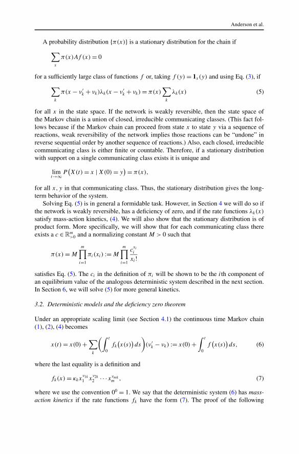
A probability distribution {π(x)} is a stationary distribution for the chain if

∑

x

π(x)Af (x) = 0

for a sufficiently large class of functions f or, taking f (y) = 1x(y) and using Eq. (3), if

∑

k

π(x − ν ′k + νk)λk(x − ν ′

k + νk) = π(x)∑

k

λk(x) (5)

for all x in the state space. If the network is weakly reversible, then the state space ofthe Markov chain is a union of closed, irreducible communicating classes. (This fact fol-lows because if the Markov chain can proceed from state x to state y via a sequence ofreactions, weak reversibility of the network implies those reactions can be “undone” inreverse sequential order by another sequence of reactions.) Also, each closed, irreduciblecommunicating class is either finite or countable. Therefore, if a stationary distributionwith support on a single communicating class exists it is unique and

limt→∞P

(X(t) = x | X(0) = y

) = π(x),

for all x, y in that communicating class. Thus, the stationary distribution gives the long-term behavior of the system.

Solving Eq. (5) is in general a formidable task. However, in Section 4 we will do so ifthe network is weakly reversible, has a deficiency of zero, and if the rate functions λk(x)

satisfy mass-action kinetics, (4). We will also show that the stationary distribution is ofproduct form. More specifically, we will show that for each communicating class thereexists a c ∈ R

m>0 and a normalizing constant M > 0 such that

π(x) = M

m∏

i=1

πi(xi) := M

m∏

i=1

cxi

i

xi !

satisfies Eq. (5). The ci in the definition of πi will be shown to be the ith component ofan equilibrium value of the analogous deterministic system described in the next section.In Section 6, we will solve (5) for more general kinetics.

3.2. Deterministic models and the deficiency zero theorem

Under an appropriate scaling limit (see Section 4.1) the continuous time Markov chain(1), (2), (4) becomes

x(t) = x(0) +∑

k

(∫ t

0fk

(x(s)

)ds

)

(ν ′k − νk) := x(0) +

∫ t

0f

(x(s)

)ds, (6)

where the last equality is a definition and

fk(x) = κkxν1k

1 xν2k

2 · · ·xνmkm , (7)

where we use the convention 00 = 1. We say that the deterministic system (6) has mass-action kinetics if the rate functions fk have the form (7). The proof of the following


theorem by Feinberg can be found in Feinberg (1979) or Feinberg (1995). We note thatthe full statement of the deficiency zero theorem actually says more than what is givenbelow and the interested reader is encouraged to see the original work.

Theorem 3.1 (The Deficiency Zero Theorem). Consider a weakly reversible, deficiencyzero chemical reaction network {S, C, R} with dynamics given by (6)–(7). Then for anychoice of rate constants {κk}, within each positive stoichiometric compatibility class thereis precisely one equilibrium value, and that equilibrium value is locally asymptoticallystable relative to its compatibility class.

The dynamics of the system (6)–(7) take place in Rm≥0. However, to prove the deficiency

zero theorem, it turns out to be more appropriate to work in complex space, denoted RC ,

which we will describe now. For any U ⊆ C, let ωU : C → {0,1} denote the indicatorfunction ωU(νk) = 1{νk∈U}. Complex space is defined to be the vector space with basis{ωνk

| νk ∈ C}, where we have denoted ω{νk} by ωνk.

If u is a vector with nonnegative integer components and w is a vector with nonneg-ative real components, then let u! = ∏

i ui ! and wu = ∏i w

ui

i , where we interpret 00 = 1and 0! = 1. Let Ψ : R

m → RC and Aκ : R

C → RC be defined by

Ψ (x) =∑

νk∈C

xνkωνk,

Aκ(y) =∑

νk→ν′k∈R

κkyνk(ων′

k− ωνk

),

where the subscript κ of Aκ denotes the choice of rate constants for the system. LetY : R

C → Rm be the linear map whose action on the basis elements {ωνk

} is defined byY (ωνk

) = νk . Then Eqs. (6)–(7) can be written as the coupled set of ordinary differentialequations

x(t) = f(x(t)

) = Y(Aκ

(Ψ

(x(t)

))).

Therefore, in order to show that a value c is an equilibrium of the system, it is sufficientto show that Aκ(Ψ (c)) = 0, which is an explicit system of equations for c. In particular,Ak(Ψ (c)) = 0 if and only if for each z ∈ C

∑

{k:ν′k=z}

κkcνk =

∑

{k:νk=z}κkc

νk , (8)

where the sum on the left is over reactions for which z is the product complex and thesum on the right is over reactions for which z is the source complex.

The following has been shown in Horn and Jackson (1972) and Feinberg (1979) (seealso Gunawardena, 2003).

Theorem 3.2. Let {S, C, R} be a chemical reaction network with dynamics given by(6)–(7) for some choice of rate constants, {κk}. Suppose there exists a c ∈ R

m>0 for which

Aκ(Ψ (c)) = 0, then the following hold:

Anderson et al.

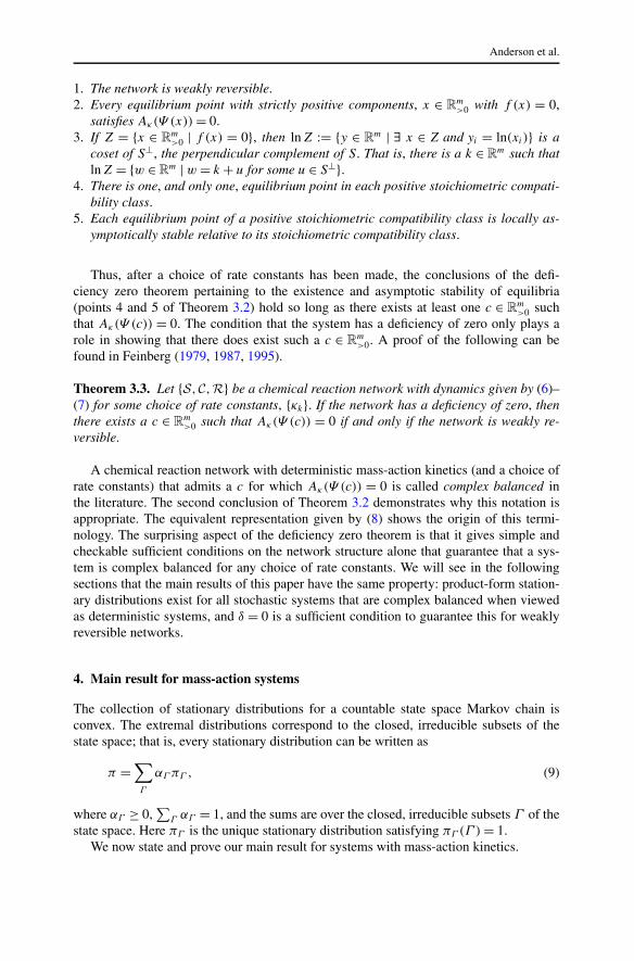
1. The network is weakly reversible.2. Every equilibrium point with strictly positive components, x ∈ R

m>0 with f (x) = 0,

satisfies Aκ(Ψ (x)) = 0.3. If Z = {x ∈ R

m>0 | f (x) = 0}, then lnZ := {y ∈ R

m | ∃ x ∈ Z and yi = ln(xi)} is acoset of S⊥, the perpendicular complement of S. That is, there is a k ∈ R

m such thatlnZ = {w ∈ R

m | w = k + u for some u ∈ S⊥}.4. There is one, and only one, equilibrium point in each positive stoichiometric compati-

bility class.5. Each equilibrium point of a positive stoichiometric compatibility class is locally as-

ymptotically stable relative to its stoichiometric compatibility class.

Thus, after a choice of rate constants has been made, the conclusions of the defi-ciency zero theorem pertaining to the existence and asymptotic stability of equilibria(points 4 and 5 of Theorem 3.2) hold so long as there exists at least one c ∈ R

m>0 such

that Aκ(Ψ (c)) = 0. The condition that the system has a deficiency of zero only plays arole in showing that there does exist such a c ∈ R

m>0. A proof of the following can be

found in Feinberg (1979, 1987, 1995).

Theorem 3.3. Let {S, C, R} be a chemical reaction network with dynamics given by (6)–(7) for some choice of rate constants, {κk}. If the network has a deficiency of zero, thenthere exists a c ∈ R

m>0 such that Aκ(Ψ (c)) = 0 if and only if the network is weakly re-

versible.

A chemical reaction network with deterministic mass-action kinetics (and a choice ofrate constants) that admits a c for which Aκ(Ψ (c)) = 0 is called complex balanced inthe literature. The second conclusion of Theorem 3.2 demonstrates why this notation isappropriate. The equivalent representation given by (8) shows the origin of this termi-nology. The surprising aspect of the deficiency zero theorem is that it gives simple andcheckable sufficient conditions on the network structure alone that guarantee that a sys-tem is complex balanced for any choice of rate constants. We will see in the followingsections that the main results of this paper have the same property: product-form station-ary distributions exist for all stochastic systems that are complex balanced when viewedas deterministic systems, and δ = 0 is a sufficient condition to guarantee this for weaklyreversible networks.

4. Main result for mass-action systems

The collection of stationary distributions for a countable state space Markov chain isconvex. The extremal distributions correspond to the closed, irreducible subsets of thestate space; that is, every stationary distribution can be written as

π =∑

Γ

αΓ πΓ , (9)

where αΓ ≥ 0,∑

Γ αΓ = 1, and the sums are over the closed, irreducible subsets Γ of thestate space. Here πΓ is the unique stationary distribution satisfying πΓ (Γ ) = 1.

We now state and prove our main result for systems with mass-action kinetics.


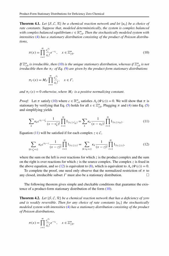
Theorem 4.1. Let {S, C, R} be a chemical reaction network and let {κk} be a choice ofrate constants. Suppose that, modeled deterministically, the system is complex balancedwith complex balanced equilibrium c ∈ R

m>0. Then the stochastically modeled system with

intensities (4) has a stationary distribution consisting of the product of Poisson distribu-tions,

π(x) =m∏

i=1

cxi

i

xi ! e−ci , x ∈ Z

m≥0. (10)

If Zm≥0 is irreducible, then (10) is the unique stationary distribution, whereas if Z

m≥0 is not

irreducible then the πΓ of Eq. (9) are given by the product-form stationary distributions

πΓ (x) = MΓ

m∏

i=1

cxi

i

xi ! , x ∈ Γ,

and πΓ (x) = 0 otherwise, where MΓ is a positive normalizing constant.

Proof: Let π satisfy (10) where c ∈ Rm>0 satisfies Aκ(Ψ (c)) = 0. We will show that π is

stationary by verifying that Eq. (5) holds for all x ∈ Zm≥0. Plugging π and (4) into Eq. (5)

and simplifying yields

∑

k

κkcνk−ν′

k1

(x − ν ′k)!

m∏

�=1

1{x�≥ν′�k

} =∑

k

κk

1

(x − νk)!m∏

�=1

1{x�≥ν�k}. (11)

Equation (11) will be satisfied if for each complex z ∈ C ,

∑

{k:ν′k=z}

κkcνk−z 1

(x − z)!m∏

�=1

1{x�≥z�} =∑

{k:νk=z}κk

1

(x − z)!m∏

�=1

1{x�≥z�}, (12)

where the sum on the left is over reactions for which z is the product complex and the sumon the right is over reactions for which z is the source complex. The complex z is fixed inthe above equation, and so (12) is equivalent to (8), which is equivalent to Aκ(Ψ (c)) = 0.

To complete the proof, one need only observe that the normalized restriction of π toany closed, irreducible subset Γ must also be a stationary distribution. �

The following theorem gives simple and checkable conditions that guarantee the exis-tence of a product-form stationary distribution of the form (10).

Theorem 4.2. Let {S, C, R} be a chemical reaction network that has a deficiency of zeroand is weakly reversible. Then for any choice of rate constants {κk} the stochasticallymodeled system with intensities (4) has a stationary distribution consisting of the productof Poisson distributions,

π(x) =m∏

i=1

cxi

i


m≥0,

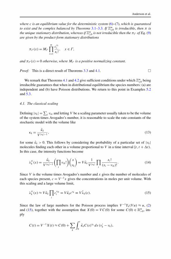
Anderson et al.

where c is an equilibrium value for the deterministic system (6)–(7), which is guaranteedto exist and be complex balanced by Theorems 3.1–3.3. If Z

m≥0 is irreducible, then π is

the unique stationary distribution, whereas if Zm≥0 is not irreducible then the πΓ of Eq. (9)

are given by the product-form stationary distributions

πΓ (x) = MΓ

m∏

i=1

cxi

i

xi ! , x ∈ Γ,


Proof: This is a direct result of Theorems 3.3 and 4.1. �

We remark that Theorems 4.1 and 4.2 give sufficient conditions under which Zm≥0 being

irreducible guarantees that when in distributional equilibrium the species numbers: (a) areindependent and (b) have Poisson distributions. We return to this point in Examples 5.2and 5.3.

4.1. The classical scaling

Defining |νk| = ∑i νik and letting V be a scaling parameter usually taken to be the volume

of the system times Avogadro’s number, it is reasonable to scale the rate constants of thestochastic model with the volume like

κk = κk

V |νk |−1, (13)

for some κk > 0. This follows by considering the probability of a particular set of |νk|molecules finding each other in a volume proportional to V in a time interval [t, t + �t).In this case, the intensity functions become

λVk (x) = κk

V |νk |−1

(∏

i

νik!)(

x

νk

)

= V κk

1

V |νk |∏

i

xi !(xi − νik)! . (14)

Since V is the volume times Avogadro’s number and x gives the number of molecules ofeach species present, c = V −1x gives the concentrations in moles per unit volume. Withthis scaling and a large volume limit,

λVk (x) ≈ V κk

∏

i

cνik

i = V κkcνk ≡ V λk(c). (15)

Since the law of large numbers for the Poisson process implies V −1Yk(V u) ≈ u, (2)and (15), together with the assumption that X(0) = V C(0) for some C(0) ∈ R

m>0, im-

ply

C(t) = V −1X(t) ≈ C(0) +∑

k

∫ t

0κkC(s)νk ds (ν ′

k − νk),


which in the large volume limit gives the classical deterministic law of mass action de-tailed in Section 3.2. For a precise formulation of the above scaling argument, termed the“classical scaling”; see Kurtz (1972, 1977/1978, 1981).

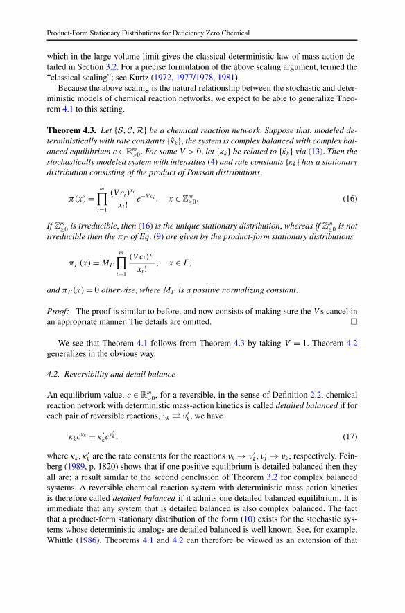
Because the above scaling is the natural relationship between the stochastic and deter-ministic models of chemical reaction networks, we expect to be able to generalize Theo-rem 4.1 to this setting.

Theorem 4.3. Let {S, C, R} be a chemical reaction network. Suppose that, modeled de-terministically with rate constants {κk}, the system is complex balanced with complex bal-anced equilibrium c ∈ R

m>0. For some V > 0, let {κk} be related to {κk} via (13). Then the

stochastically modeled system with intensities (4) and rate constants {κk} has a stationarydistribution consisting of the product of Poisson distributions,

π(x) =m∏

i=1

(V ci)xi

xi ! e−V ci , x ∈ Zm≥0. (16)

If Zm≥0 is irreducible, then (16) is the unique stationary distribution, whereas if Z

m≥0 is not

irreducible then the πΓ of Eq. (9) are given by the product-form stationary distributions

πΓ (x) = MΓ

m∏

i=1

(V ci)xi

xi ! , x ∈ Γ,


Proof: The proof is similar to before, and now consists of making sure the V s cancel inan appropriate manner. The details are omitted. �

We see that Theorem 4.1 follows from Theorem 4.3 by taking V = 1. Theorem 4.2generalizes in the obvious way.

4.2. Reversibility and detail balance

An equilibrium value, c ∈ Rm>0, for a reversible, in the sense of Definition 2.2, chemical

reaction network with deterministic mass-action kinetics is called detailed balanced if foreach pair of reversible reactions, νk � ν ′

k , we have

κkcνk = κ ′

kcν′k , (17)

where κk, κ′k are the rate constants for the reactions νk → ν ′

k, ν′k → νk , respectively. Fein-

berg (1989, p. 1820) shows that if one positive equilibrium is detailed balanced then theyall are; a result similar to the second conclusion of Theorem 3.2 for complex balancedsystems. A reversible chemical reaction system with deterministic mass action kineticsis therefore called detailed balanced if it admits one detailed balanced equilibrium. It isimmediate that any system that is detailed balanced is also complex balanced. The factthat a product-form stationary distribution of the form (10) exists for the stochastic sys-tems whose deterministic analogs are detailed balanced is well known. See, for example,Whittle (1986). Theorems 4.1 and 4.2 can therefore be viewed as an extension of that

Anderson et al.

result. However, more can be said in the case when the deterministic system is detailedbalanced, and which we include here for completeness (no originality is being claimed).

As mentioned in the remark following Definition 2.2, the term “reversible” has a mean-ing in the context of stochastic processes that differs from that of Definition 2.2. Beforedefining this, we need the concept of a transition rate. For any continuous time Markovchain with state space Γ , the transition rate from x ∈ Γ to y ∈ Γ (with x �= y) is a non-negative number α(x, y) satisfying

P(X(t + �t) = y | X(t) = x

) = α(x, y)�t + o(�t).

Thus, in the context of this paper, if y = x + ν ′k − νk for some k, then α(x, y) = λk(x),

and zero otherwise.

Definition 4.4. A continuous time Markov chain X(t) with transition rates α(x, y) isreversible with respect to the distribution π if for all x, y in the state space Γ

π(x)α(x, y) = π(y)α(y, x). (18)

It is simple to see (by summing both sides of (18) with respect to y over Γ ), that π

must be a stationary distribution for the process. A stationary distribution satisfying (18)is even called detailed balanced in the probability literature. The following is proved inWhittle (1986, Chap. 7).

Theorem 4.5. Let {S, C, R} be a reversible2 chemical reaction network with rate con-stants {κk}. Then the deterministically modeled system with mass-action kinetics has adetailed balanced equilibrium if and only if the stochastically modeled system with inten-sities (4) is reversible with respect to its stationary distribution.3

Succinctly, this theorem says that reversibility and detailed balanced in the determin-istic setting is equivalent to reversible (and hence, detailed balanced) in the stochasticsetting.

4.3. Non-uniqueness of c

For stochastically modeled chemical reaction systems any irreducible subset of the statespace, Γ , is contained within (y + S) ∩ Z

m≥0 for some y ∈ R

m≥0. Therefore, each Γ is as-

sociated with a stoichiometric compatibility class. For weakly reversible systems with adeficiency of zero, Theorems 3.2 and 3.3 guarantee that each such stoichiometric com-patibility class has an associated equilibrium value for which Aκ(Ψ (c)) = 0. However,neither Theorem 4.1 nor Theorem 4.2 makes the requirement that the equilibrium valueused in the product-form stationary measure πΓ (·) be contained within the stoichiomet-ric compatibility class associated with Γ . Therefore, we see that one such c can be usedto construct a product-form stationary distribution for every closed, irreducible subset.Conversely, for a given irreducible subset Γ any positive equilibrium value of the system

2In the sense of Definition 2.2.3In the sense of Definition 4.4.


(6)–(7) can be used to construct πΓ (·). This fact seems to be contrary to the uniquenessof the stationary distribution; however, it can be understood through the third conclusionof Theorem 3.2 as follows.

Let Γ be a closed, irreducible subset of the state space with associated positivestoichiometric compatibility class (y + S) ∩ Z

m≥0, and let c1, c2 ∈ R

m>0 be such that

Aκ(Ψ (c1)) = Aκ(Ψ (c2)) = 0. For i ∈ {1,2} and x ∈ Γ , let πi(x) = Micxi /x!, where M1

and M2 are normalizing constants. Then for each x ∈ Γ

π1(x)

π2(x)= M1c

x1

x!x!

M2cx2

= M1

M2

cx1

cx2

.

For any vector u, we define (ln(u))i = ln(ui). Then for x ∈ Γ ⊂ y + S

cx1

cx2

= ex·(ln c1−ln c2) = ey·(ln c1−ln c2) = cy

1

cy

2

, (19)

where the second equality follows from the third conclusion of Theorem 3.2. Therefore,

π1(x)

π2(x)= M1

M2

cy

1

cy

2

. (20)

Finally,

1 =(

M1

∑

x∈Γ

cx1/x!

)/(

M2

∑

x∈Γ

cx2/x!

)

= M1

M2

(c

y

1

cy

2

∑

x∈Γ

cx2/x!

)/(∑

x∈Γ

cx2/x!

)

= π1(x)

π2(x),

where the second equality follows from Eq. (19) and the third equality follows fromEq. (20). We therefore see that the stationary measure is independent of the choice of c,as expected.

5. Examples

Our first example points out that the existence of a product-form stationary distribution forthe closed, irreducible subsets of the state space does not necessarily imply independenceof the species numbers.

Example 5.1 (Nonindependence of species numbers). Consider the simple reversible sys-tem

S1

k1�k2

S2,

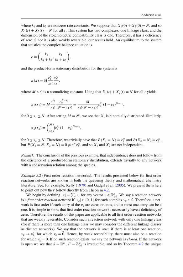
Anderson et al.

where k1 and k2 are nonzero rate constants. We suppose that X1(0) + X2(0) = N , and soX1(t) + X2(t) = N for all t . This system has two complexes, one linkage class, and thedimension of the stoichiometric compatibility class is one. Therefore, it has a deficiencyof zero. Since it is also weakly reversible, our results hold. An equilibrium to the systemthat satisfies the complex balance equation is

c =(

k2

k1 + k2,

k1

k1 + k2

)

,

and the product-form stationary distribution for the system is

π(x) = Mc

x11

x1!c

x22

x2! ,

where M > 0 is a normalizing constant. Using that X1(t) + X2(t) = N for all t yields

π1(x1) = Mc

x11

x1!c

N−x12

(N − x1)! = M

x1!(N − x1)!cx11 (1 − c1)

N−x1 ,

for 0 ≤ x1 ≤ N . After setting M = N !, we see that X1 is binomially distributed. Similarly,

π2(x2) =(

N

x2

)

cx22 (1 − c2)

N−x2 ,

for 0 ≤ x2 ≤ N . Therefore, we trivially have that P (X1 = N) = cN1 and P (X2 = N) = cN

2 ,but P (X1 = N,X2 = N) = 0 �= cN

1 cN2 , and so X1 and X2 are not independent.

Remark. The conclusion of the previous example, that independence does not follow fromthe existence of a product-form stationary distribution, extends trivially to any networkwith a conservation relation among the species.

Example 5.2 (First order reaction networks). The results presented below for first orderreaction networks are known in both the queueing theory and mathematical chemistryliterature. See, for example, Kelly (1979) and Gadgil et al. (2005). We present them hereto point out how they follow directly from Theorem 4.2.

We begin by defining |v| = ∑i vi for any vector v ∈ R

m≥0. We say a reaction network

is a first order reaction network if |νk| ∈ {0,1} for each complex νk ∈ C . Therefore, a net-work is first order if each entry of the νk are zeros or ones, and at most one entry can be aone. It is simple to show that first order reaction networks necessarily have a deficiency ofzero. Therefore, the results of this paper are applicable to all first order reaction networksthat are weakly reversible. Consider such a reaction network with only one linkage class(for if there is more than one linkage class we may consider the different linkage classesas distinct networks). We say that the network is open if there is at least one reaction,νk → ν ′

k , for which νk = �0. Hence, by weak reversibility, there must also be a reactionfor which ν ′

k = �0. If no such reaction exists, we say the network is closed. If the networkis open we see that S = R

m, Γ = Zm≥0 is irreducible, and so by Theorem 4.2 the unique


stationary distribution is

π(x) =m∏

i=1

cxi

i


m≥0,

where c ∈ Rm>0 is the complexed balanced equilibrium of the associated (linear) deter-

ministic system. Therefore, when in distributional equilibrium, the species numbers areindependent and have Poisson distributions. Note that neither the independence nor thePoisson distribution resulted from the fact that the system under consideration was a firstorder system. Instead both facts followed from Γ being all of Z

m≥0.

In the case of a closed, weakly reversible, single linkage class, first order reaction net-work, it is easy to see that there is a unique conservation relation X1(t)+· · ·+Xm(t) = N ,for some N . Thus, in distributional equilibrium X(t) has a multinomial distribution. Thatis for any x ∈ Z

m≥0 satisfying x1 + x2 + · · · + xm = N

π(x) =(

N

x1, x2, . . . , xm

)

cx = N !x1! · · ·xm!c

x11 · · · cxm

m , (21)

where c ∈ Rm>0 is the equilibrium of the associated deterministic system normalized so that∑

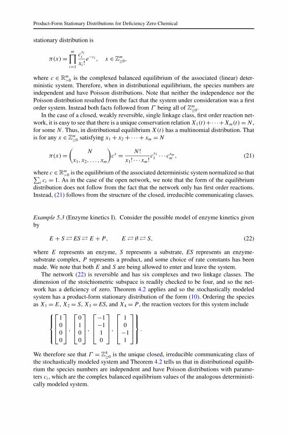
i ci = 1. As in the case of the open network, we note that the form of the equilibriumdistribution does not follow from the fact that the network only has first order reactions.Instead, (21) follows from the structure of the closed, irreducible communicating classes.

Example 5.3 (Enzyme kinetics I). Consider the possible model of enzyme kinetics givenby

E + S � ES � E + P, E � ∅ � S, (22)

where E represents an enzyme, S represents a substrate, ES represents an enzyme-substrate complex, P represents a product, and some choice of rate constants has beenmade. We note that both E and S are being allowed to enter and leave the system.

The network (22) is reversible and has six complexes and two linkage classes. Thedimension of the stoichiometric subspace is readily checked to be four, and so the net-work has a deficiency of zero. Theorem 4.2 applies and so the stochastically modeledsystem has a product-form stationary distribution of the form (10). Ordering the speciesas X1 = E, X2 = S, X3 = ES, and X4 = P , the reaction vectors for this system include

⎧⎪⎪⎨

⎪⎪⎩

⎡

⎢⎢⎣

1000

⎤

⎥⎥⎦ ,

⎡

⎢⎢⎣

0100

⎤

⎥⎥⎦ ,

⎡

⎢⎢⎣

−1−110

⎤

⎥⎥⎦ ,

⎡

⎢⎢⎣

10

−11

⎤

⎥⎥⎦

⎫⎪⎪⎬

⎪⎪⎭.

We therefore see that Γ = Z4≥0 is the unique closed, irreducible communicating class of

the stochastically modeled system and Theorem 4.2 tells us that in distributional equilib-rium the species numbers are independent and have Poisson distributions with parame-ters ci , which are the complex balanced equilibrium values of the analogous deterministi-cally modeled system.

Anderson et al.

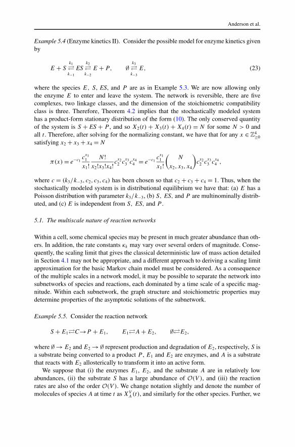
Example 5.4 (Enzyme kinetics II). Consider the possible model for enzyme kinetics givenby

E + Sk1�k−1

ESk2�k−2

E + P, ∅k3�k−3

E, (23)

where the species E, S, ES, and P are as in Example 5.3. We are now allowing onlythe enzyme E to enter and leave the system. The network is reversible, there are fivecomplexes, two linkage classes, and the dimension of the stoichiometric compatibilityclass is three. Therefore, Theorem 4.2 implies that the stochastically modeled systemhas a product-form stationary distribution of the form (10). The only conserved quantityof the system is S + ES + P , and so X2(t) + X3(t) + X4(t) = N for some N > 0 andall t . Therefore, after solving for the normalizing constant, we have that for any x ∈ Z

4≥0

satisfying x2 + x3 + x4 = N

π(x) = e−c1c

x11

x1!N !

x2!x3!x4!cx22 c

x33 c

x44 = e−c1

cx11

x1!(

N

x2, x3, x4

)

cx22 c

x33 c

x44 ,

where c = (k3/k−3, c2, c3, c4) has been chosen so that c2 + c3 + c4 = 1. Thus, when thestochastically modeled system is in distributional equilibrium we have that: (a) E has aPoisson distribution with parameter k3/k−3, (b) S, ES, and P are multinominally distrib-uted, and (c) E is independent from S, ES, and P .

5.1. The multiscale nature of reaction networks

Within a cell, some chemical species may be present in much greater abundance than oth-ers. In addition, the rate constants κk may vary over several orders of magnitude. Conse-quently, the scaling limit that gives the classical deterministic law of mass action detailedin Section 4.1 may not be appropriate, and a different approach to deriving a scaling limitapproximation for the basic Markov chain model must be considered. As a consequenceof the multiple scales in a network model, it may be possible to separate the network intosubnetworks of species and reactions, each dominated by a time scale of a specific mag-nitude. Within each subnetwork, the graph structure and stoichiometric properties maydetermine properties of the asymptotic solutions of the subnetwork.

Example 5.5. Consider the reaction network

S + E1�C→P + E1, E1�A + E2, ∅�E2,

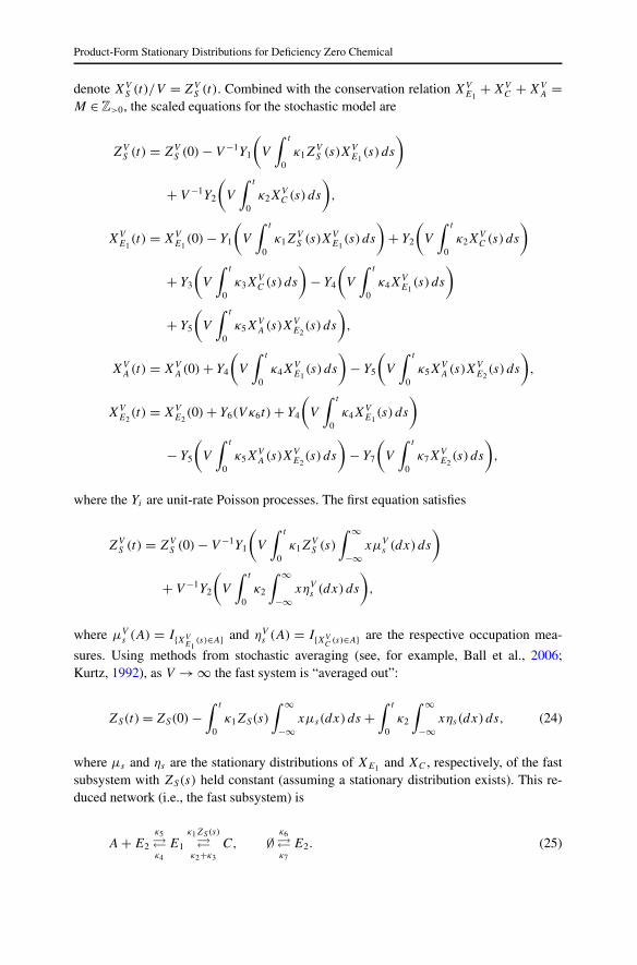
where ∅ → E2 and E2 → ∅ represent production and degradation of E2, respectively, S isa substrate being converted to a product P , E1 and E2 are enzymes, and A is a substratethat reacts with E2 allosterically to transform it into an active form.

We suppose that (i) the enzymes E1, E2, and the substrate A are in relatively lowabundances, (ii) the substrate S has a large abundance of O(V ), and (iii) the reactionrates are also of the order O(V ). We change notation slightly and denote the number ofmolecules of species A at time t as XV

A(t), and similarly for the other species. Further, we


denote XVS (t)/V = ZV

S (t). Combined with the conservation relation XVE1

+ XVC + XV

A =M ∈ Z>0, the scaled equations for the stochastic model are

ZVS (t) = ZV

S (0) − V −1Y1

(

V

∫ t

0κ1Z

VS (s)XV

E1(s) ds

)

+ V −1Y2

(

V

∫ t

0κ2X

VC (s) ds

)

,

XVE1

(t) = XVE1

(0) − Y1

(

V

∫ t

0κ1Z

VS (s)XV

E1(s) ds

)

+ Y2

(

V

∫ t

0κ2X

VC (s) ds

)

+ Y3

(

V

∫ t

0κ3X

VC (s) ds

)

− Y4

(

V

∫ t

0κ4X

VE1

(s) ds

)

+ Y5

(

V

∫ t

0κ5X

VA(s)XV

E2(s) ds

)

,

XVA(t) = XV

A(0) + Y4

(

V

∫ t

0κ4X

VE1

(s) ds

)

− Y5

(

V

∫ t

0κ5X

VA(s)XV

E2(s) ds

)

,

XVE2

(t) = XVE2

(0) + Y6(V κ6t) + Y4

(

V

∫ t

0κ4X

VE1

(s) ds

)

− Y5

(

V

∫ t

0κ5X

VA(s)XV

E2(s) ds

)

− Y7

(

V

∫ t

0κ7X

VE2

(s) ds

)

,

where the Yi are unit-rate Poisson processes. The first equation satisfies

ZVS (t) = ZV

S (0) − V −1Y1

(

V

∫ t

0κ1Z

VS (s)

∫ ∞

−∞xμV

s (dx) ds

)

+ V −1Y2

(

V

∫ t

0κ2

∫ ∞

−∞xηV

s (dx) ds

)

,

where μVs (A) = I{XV

E1(s)∈A} and ηV

s (A) = I{XVC

(s)∈A} are the respective occupation mea-

sures. Using methods from stochastic averaging (see, for example, Ball et al., 2006;Kurtz, 1992), as V → ∞ the fast system is “averaged out”:

ZS(t) = ZS(0) −∫ t

0κ1ZS(s)

∫ ∞

−∞xμs(dx)ds +

∫ t

0κ2

∫ ∞

−∞xηs(dx) ds, (24)

where μs and ηs are the stationary distributions of XE1 and XC , respectively, of the fastsubsystem with ZS(s) held constant (assuming a stationary distribution exists). This re-duced network (i.e., the fast subsystem) is

A + E2

κ5�κ4

E1

κ1ZS(s)

�κ2+κ3

C, ∅κ6�κ7

E2. (25)

Anderson et al.

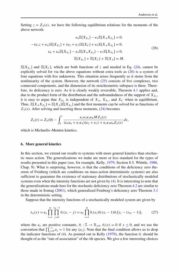
Setting z = ZS(s), we have the following equilibrium relations for the moments of theabove network:

κ4E[XE1 ] − κ5E[XAXE2 ] = 0,

−(κ1z + κ4)E[XE1 ] + (κ2 + κ3)E[XC] + κ5E[XAXE2 ] = 0,

κ6 + κ4E[XE1 ] − κ5E[XAXE2 ] − κ7E[XE2 ] = 0,

E[XE1 ] + E[XC] + E[XA] = M.

(26)

E[XE1 ] and E[XC], which are both functions of z and needed in Eq. (24), cannot beexplicitly solved for via the above equations without extra tools as (26) is a system offour equations with five unknowns. This situation arises frequently as it stems from thenonlinearity of the system. However, the network (25) consists of five complexes, twoconnected components, and the dimension of its stoichiometric subspace is three. There-fore, its deficiency is zero. As it is clearly weakly reversible, Theorem 4.1 applies and,due to the product form of the distribution and the unboundedness of the support of XE2 ,it is easy to argue that XE2 is independent of XA, XE1 , and XC when in equilibrium.Thus, E[XAXE2 ] = E[XA]E[XE2 ] and the first moments can be solved for as functions ofZS(s). After solving and inserting these moments, (24) becomes

ZS(t) = ZS(0) −∫ t

0

κ1κ3κ5κ6MZS(s)

(κ5κ6 + κ7κ4)(κ2 + κ3) + κ1κ5κ6ZS(s)ds,

which is Michaelis–Menten kinetics.

6. More general kinetics

In this section, we extend our results to systems with more general kinetics than stochas-tic mass action. The generalizations we make are more or less standard for the types ofresults presented in this paper (see, for example, Kelly, 1979, Section 8.5, Whittle, 1986,Chap. 9). What is surprising, however, is that the conditions of the deficiency zero the-orem of Feinberg (which are conditions on mass-action deterministic systems) are alsosufficient to guarantee the existence of stationary distributions of stochastically modeledsystems even when the intensity functions are not given by (4). It is interesting to note thatthe generalizations made here for the stochastic deficiency zero Theorem 4.2 are similar tothose made in Sontag (2001), which generalized Feinberg’s deficiency zero Theorem 3.1in the deterministic setting.

Suppose that the intensity functions of a stochastically modeled system are given by

λk(x) = κk

m∏

i=1

νik−1∏

j=0

θi(xi − j) = κk

m∏

i=1

θi(xi)θi(xi − 1)θi

(xi − (νik − 1)

), (27)

where the κk are positive constants, θi : Z → R≥0, θi(x) = 0 if x ≤ 0, and we use theconvention that

∏−1j=0 aj = 1 for any {aj }. Note that the final condition allows us to drop

the indicator functions of (4). As pointed out in Kelly (1979), the function θi should bethought of as the “rate of association” of the ith species. We give a few interesting choices


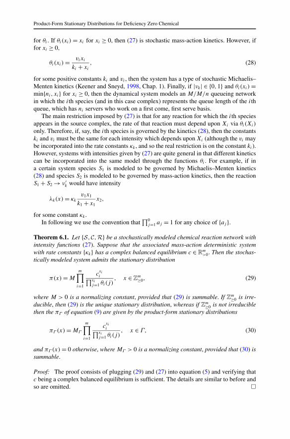
for θi . If θi(xi) = xi for xi ≥ 0, then (27) is stochastic mass-action kinetics. However, iffor xi ≥ 0,

θi(xi) = vixi

ki + xi

, (28)

for some positive constants ki and vi , then the system has a type of stochastic Michaelis–Menten kinetics (Keener and Sneyd, 1998, Chap. 1). Finally, if |νk| ∈ {0,1} and θi(xi) =min{ni, xi} for xi ≥ 0, then the dynamical system models an M/M/n queueing networkin which the ith species (and in this case complex) represents the queue length of the ithqueue, which has ni servers who work on a first come, first serve basis.

The main restriction imposed by (27) is that for any reaction for which the ith speciesappears in the source complex, the rate of that reaction must depend upon Xi via θi(Xi)

only. Therefore, if, say, the ith species is governed by the kinetics (28), then the constantski and vi must be the same for each intensity which depends upon Xi (although the vi maybe incorporated into the rate constants κk , and so the real restriction is on the constant ki ).However, systems with intensities given by (27) are quite general in that different kineticscan be incorporated into the same model through the functions θi . For example, if ina certain system species S1 is modeled to be governed by Michaelis–Menten kinetics(28) and species S2 is modeled to be governed by mass-action kinetics, then the reactionS1 + S2 → ν ′

k would have intensity

λk(x) = κk

v1x1

k1 + x1x2,

for some constant κk .In following we use the convention that

∏0j=1 aj = 1 for any choice of {aj }.

Theorem 6.1. Let {S, C, R} be a stochastically modeled chemical reaction network withintensity functions (27). Suppose that the associated mass-action deterministic systemwith rate constants {κk} has a complex balanced equilibrium c ∈ R

m>0. Then the stochas-

tically modeled system admits the stationary distribution

π(x) = M

m∏

i=1

cxi

i∏xi

j=1 θi(j), x ∈ Z

m≥0, (29)

where M > 0 is a normalizing constant, provided that (29) is summable. If Zm≥0 is irre-

ducible, then (29) is the unique stationary distribution, whereas if Zm≥0 is not irreducible

then the πΓ of equation (9) are given by the product-form stationary distributions

πΓ (x) = MΓ

m∏

i=1

cxi

i∏xi

j=1 θi(j), x ∈ Γ, (30)

and πΓ (x) = 0 otherwise, where MΓ > 0 is a normalizing constant, provided that (30) issummable.

Proof: The proof consists of plugging (29) and (27) into equation (5) and verifying thatc being a complex balanced equilibrium is sufficient. The details are similar to before andso are omitted. �

Anderson et al.

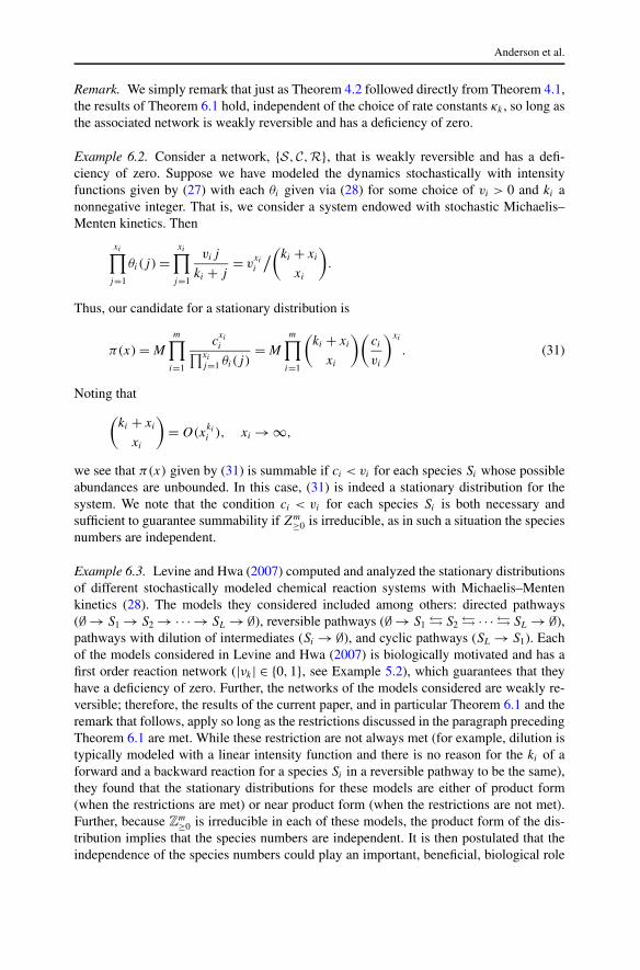
Remark. We simply remark that just as Theorem 4.2 followed directly from Theorem 4.1,the results of Theorem 6.1 hold, independent of the choice of rate constants κk , so long asthe associated network is weakly reversible and has a deficiency of zero.

Example 6.2. Consider a network, {S, C, R}, that is weakly reversible and has a defi-ciency of zero. Suppose we have modeled the dynamics stochastically with intensityfunctions given by (27) with each θi given via (28) for some choice of vi > 0 and ki anonnegative integer. That is, we consider a system endowed with stochastic Michaelis–Menten kinetics. Then

xi∏

j=1

θi(j) =xi∏

j=1

vij

ki + j= v

xi

i

/(

ki + xi

xi

)

.

Thus, our candidate for a stationary distribution is

π(x) = M

m∏

i=1

cxi

i∏xi

j=1 θi(j)= M

m∏

i=1

(ki + xi

xi

)(ci

vi

)xi

. (31)

Noting that

(ki + xi

xi

)

= O(xki

i ), xi → ∞,

we see that π(x) given by (31) is summable if ci < vi for each species Si whose possibleabundances are unbounded. In this case, (31) is indeed a stationary distribution for thesystem. We note that the condition ci < vi for each species Si is both necessary andsufficient to guarantee summability if Zm

≥0 is irreducible, as in such a situation the speciesnumbers are independent.

Example 6.3. Levine and Hwa (2007) computed and analyzed the stationary distributionsof different stochastically modeled chemical reaction systems with Michaelis–Mentenkinetics (28). The models they considered included among others: directed pathways(∅ → S1 → S2 → ·· · → SL → ∅), reversible pathways (∅ → S1 � S2 � · · · � SL → ∅),pathways with dilution of intermediates (Si → ∅), and cyclic pathways (SL → S1). Eachof the models considered in Levine and Hwa (2007) is biologically motivated and has afirst order reaction network (|νk| ∈ {0,1}, see Example 5.2), which guarantees that theyhave a deficiency of zero. Further, the networks of the models considered are weakly re-versible; therefore, the results of the current paper, and in particular Theorem 6.1 and theremark that follows, apply so long as the restrictions discussed in the paragraph precedingTheorem 6.1 are met. While these restriction are not always met (for example, dilution istypically modeled with a linear intensity function and there is no reason for the ki of aforward and a backward reaction for a species Si in a reversible pathway to be the same),they found that the stationary distributions for these models are either of product form(when the restrictions are met) or near product form (when the restrictions are not met).Further, because Z

m≥0 is irreducible in each of these models, the product form of the dis-

tribution implies that the species numbers are independent. It is then postulated that theindependence of the species numbers could play an important, beneficial, biological role


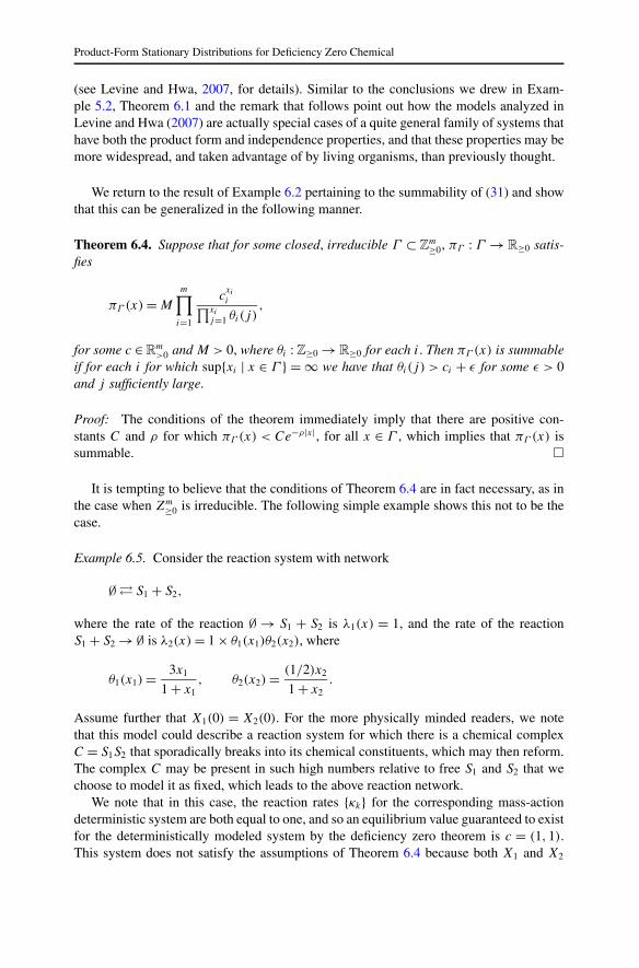
(see Levine and Hwa, 2007, for details). Similar to the conclusions we drew in Exam-ple 5.2, Theorem 6.1 and the remark that follows point out how the models analyzed inLevine and Hwa (2007) are actually special cases of a quite general family of systems thathave both the product form and independence properties, and that these properties may bemore widespread, and taken advantage of by living organisms, than previously thought.

We return to the result of Example 6.2 pertaining to the summability of (31) and showthat this can be generalized in the following manner.

Theorem 6.4. Suppose that for some closed, irreducible Γ ⊂ Zm≥0, πΓ : Γ → R≥0 satis-

fies

πΓ (x) = M

m∏

i=1

cxi

i∏xi

j=1 θi(j),

for some c ∈ Rm>0 and M > 0, where θi : Z≥0 → R≥0 for each i. Then πΓ (x) is summable

if for each i for which sup{xi | x ∈ Γ } = ∞ we have that θi(j) > ci + ε for some ε > 0and j sufficiently large.

Proof: The conditions of the theorem immediately imply that there are positive con-stants C and ρ for which πΓ (x) < Ce−ρ|x|, for all x ∈ Γ , which implies that πΓ (x) issummable. �

It is tempting to believe that the conditions of Theorem 6.4 are in fact necessary, as inthe case when Zm

≥0 is irreducible. The following simple example shows this not to be thecase.

Example 6.5. Consider the reaction system with network

∅ � S1 + S2,

where the rate of the reaction ∅ → S1 + S2 is λ1(x) = 1, and the rate of the reactionS1 + S2 → ∅ is λ2(x) = 1 × θ1(x1)θ2(x2), where

θ1(x1) = 3x1

1 + x1, θ2(x2) = (1/2)x2

1 + x2.

Assume further that X1(0) = X2(0). For the more physically minded readers, we notethat this model could describe a reaction system for which there is a chemical complexC = S1S2 that sporadically breaks into its chemical constituents, which may then reform.The complex C may be present in such high numbers relative to free S1 and S2 that wechoose to model it as fixed, which leads to the above reaction network.

We note that in this case, the reaction rates {κk} for the corresponding mass-actiondeterministic system are both equal to one, and so an equilibrium value guaranteed to existfor the deterministically modeled system by the deficiency zero theorem is c = (1,1).This system does not satisfy the assumptions of Theorem 6.4 because both X1 and X2

Anderson et al.

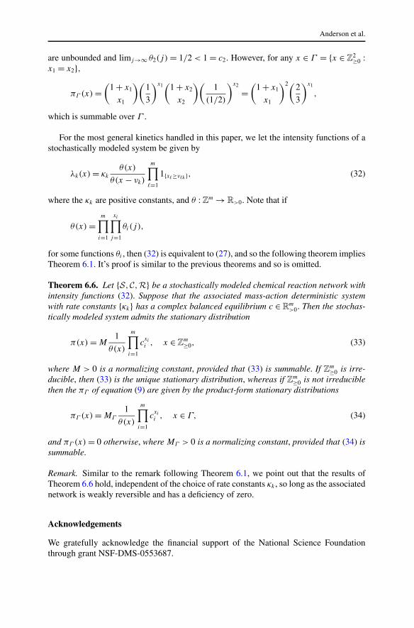
are unbounded and limj→∞ θ2(j) = 1/2 < 1 = c2. However, for any x ∈ Γ = {x ∈ Z2≥0 :

x1 = x2},

πΓ (x) =(

1 + x1

x1

)(1

3

)x1(

1 + x2

x2

)(1

(1/2)

)x2

=(

1 + x1

x1

)2(2

3

)x1

,

which is summable over Γ .

For the most general kinetics handled in this paper, we let the intensity functions of astochastically modeled system be given by

λk(x) = κk

θ(x)

θ(x − νk)

m∏

�=1

1{x�≥ν�k }, (32)

where the κk are positive constants, and θ : Zm → R>0. Note that if

θ(x) =m∏

i=1

xi∏

j=1

θi(j),

for some functions θi , then (32) is equivalent to (27), and so the following theorem impliesTheorem 6.1. It’s proof is similar to the previous theorems and so is omitted.

Theorem 6.6. Let {S, C, R} be a stochastically modeled chemical reaction network withintensity functions (32). Suppose that the associated mass-action deterministic systemwith rate constants {κk} has a complex balanced equilibrium c ∈ R

m>0. Then the stochas-

tically modeled system admits the stationary distribution

π(x) = M1

θ(x)

m∏

i=1

cxi

i , x ∈ Zm≥0, (33)

where M > 0 is a normalizing constant, provided that (33) is summable. If Zm≥0 is irre-

ducible, then (33) is the unique stationary distribution, whereas if Zm≥0 is not irreducible

then the πΓ of equation (9) are given by the product-form stationary distributions

πΓ (x) = MΓ

1

θ(x)

m∏

i=1

cxi

i , x ∈ Γ, (34)

and πΓ (x) = 0 otherwise, where MΓ > 0 is a normalizing constant, provided that (34) issummable.

Remark. Similar to the remark following Theorem 6.1, we point out that the results ofTheorem 6.6 hold, independent of the choice of rate constants κk , so long as the associatednetwork is weakly reversible and has a deficiency of zero.

Acknowledgements

We gratefully acknowledge the financial support of the National Science Foundationthrough grant NSF-DMS-0553687.


References

Anderson, D.F., 2007. A modified next reaction method for simulating chemical systems with time depen-dent propensities and delays. J. Chem. Phys. 127(21), 214107.

Anderson, D.F., 2008a. Global asymptotic stability for a class of nonlinear chemical equations. SIAM J.Appl. Math. 68, 1464–1476.

Anderson, D.F., 2008b. Incorporating postleap checks in tau-leaping. J. Chem. Phys. 128(5), 054103.Anderson, D.F., Craciun, G., 2010. Reduced reaction networks and persistence of chemical systems (in

preparation).Anderson, D.F., Shiu, A., 2010. The dynamics of weakly reversible population processes near facets. SIAM

J. Appl. Math. 70(6), 1840–1858.Anderson, D.F., Ganguly, A., Kurtz, T.G., 2010. Error analysis of tau-leap simulation methods. arXiv:

0909.4790 (submitted).Angeli, D., De Leenheer, P., Sontag, E.D., 2007. A petri net approach to the study of persistence in chem-

ical reaction networks. Math. Biosci. 210, 598–618.Ball, K., Kurtz, T.G., Popovic, L., Rempala, G., 2006. Asymptotic analysis of multiscale approximations

to reaction networks. Ann. Appl. Probab. 16(4), 1925–1961.Cao, Y., Gillespie, D.T., Petzold, L.R., 2006. Efficient step size selection for the tau-leaping simulation

method. J. Chem. Phys. 124, 044109.Chen, H., Yao, D.D., 2001. Fundamentals of Queueing Networks, Performance, Asymptotics and Op-

timization, Applications of Mathematics, Stochastic Modelling and Applied Probability, vol. 46.Springer, New York.

Craciun, G., Feinberg, M., 2005. Multiple equilibria in complex chemical reaction networks: I. The injec-tivity property. SIAM J. Appl. Math. 65(5), 1526–1546.

Craciun, G., Feinberg, M., 2006. Multiple equilibria in complex chemical reaction networks: II. Thespecies-reactions graph. SIAM J. Appl. Math. 66(4), 1321–1338.

Craciun, G., Tang, Y., Feinberg, M., 2006. Understanding bistability in complex enzyme-driven networks.Proc. Natl. Acad. Sci. USA 103(23), 8697–8702.

Ethier, S.N., Kurtz, T.G., 1986. Markov Processes: Characterization and Convergence. Wiley, New York.Feinberg, M., 1972. Complex balancing in general kinetic systems. Arch. Ration. Mech. Anal. 49, 187–

194.Feinberg, M., 1979. Lectures on chemical reaction networks. Delivered at the Mathematics Re-

search Center, Univ. Wisc.-Madison. Available for download at http://www.che.eng.ohio-state.edu/~feinberg/LecturesOnReactionNetworks.

Feinberg, M., 1987. Chemical reaction network structure and the stability of complex isothermalreactors—I. The deficiency zero and deficiency one theorems, review article 25. Chem. Eng. Sci.42, 2229–2268.

Feinberg, M., 1989. Necessary and sufficient conditions for detailed balancing in mass action systems ofarbitrary complexity. Chem. Eng. Sci. 44(9), 1819–1827.

Feinberg, M., 1995. Existence and uniqueness of steady states for a class of chemical reaction networks.Arch. Ration. Mech. Anal. 132, 311–370.

Gadgil, C., Lee, C.H., Othmer, H.G., 2005. A stochastic analysis of first-order reaction networks. Bull.Math. Biol. 67, 901–946.

Gibson, M.A., Bruck, J., 2000. Efficient exact stochastic simulation of chemical systems with many speciesand many channels. J. Phys. Chem. A 105, 1876–1889.

Gillespie, D.T., 1976. A general method for numerically simulating the stochastic time evolution of cou-pled chemical reactions. J. Comput. Phys. 22, 403–434.

Gillespie, D.T., 1977. Exact stochastic simulation of coupled chemical reactions. J. Phys. Chem. 81(25),2340–2361.

Gillespie, D.T., 2001. Approximate accelerated simulation of chemically reacting systems. J. Chem. Phys.115(4), 1716–1733.

Gunawardena, J., 2003. Chemical reaction network theory for in-silico biologists. Notes available fordownload at http://vcp.med.harvard.edu/papers/crnt.pdf.

Horn, F.J.M., 1972. Necessary and sufficient conditions for complex balancing in chemical kinetics. Arch.Ration. Mech. Anal. 49(3), 172–186.

Horn, F.J.M., 1973. Stability and complex balancing in mass-action systems with three complexes. Proc.R. Soc. A 334, 331–342.

Horn, F.J.M., Jackson, R., 1972. General mass action kinetics. Arch. Ration. Mech. Anal. 47, 81–116.

http://arxiv.org/abs/arXiv:0909.4790

http://arxiv.org/abs/arXiv:0909.4790

http://www.che.eng.ohio-state.edu/~feinberg/LecturesOnReactionNetworks

http://www.che.eng.ohio-state.edu/~feinberg/LecturesOnReactionNetworks

http://vcp.med.harvard.edu/papers/crnt.pdf

Anderson et al.

Keener, J., Sneyd, J., 1998. Mathematical Physiology. Springer, New York.Kelly, F.P., 1979. Reversibility and Stochastic Networks, Wiley Series in Probability and Mathematical

Statistics. Wiley, New York.Kurtz, T.G., 1972. The relationship between stochastic and deterministic models for chemical reactions.

J. Chem. Phys. 57(7), 2976–2978.Kurtz, T.G., 1977/1978. Strong approximation theorems for density dependent Markov chains. Stoch. Proc.

Appl. 6, 223–240.Kurtz, T.G., 1981. Approximation of Population Processes, CBMS-NSF Reg. Conf. Series in Appl. Math.,

vol. 36. SIAM, Philadelphia.Kurtz, T.G., 1992. Averaging for Martingale Problems and Stochastic Approximation, Applied Stochastic

Analysis, Lecture Notes in Control and Information Sciences, vol. 77, pp. 186–209. Springer, Berlin.Levine, E., Hwa, T., 2007. Stochastic fluctuations in metabolic pathways. Proc. Natl. Acad. Sci. USA

104(22), 9224–9229.Serfozo, R., 1999. Introduction to Stochastic Networks, Applications of Mathematics (New York), vol. 44.

Springer, New York.Sontag, E.D., 2001. Structure and stability of certain chemical networks and applications to the kinetic

proofreading of t-cell receptor signal transduction. IEEE Trans. Autom. Control. 46(7), 1028–1047.Whittle, P., 1986. Systems in Stochastic Equilibrium. Wiley, New York.

product-form stationary distributions for deﬁciency zero

Documents