Processing and Assimilation of Radar Data

Workshop on Shaping the Development of

EarthCube to Enable Advances in Data Assimilation and Ensemble

Prediction Boulder CO, 17-18, Dec 2012

Ming Xue Center for Analysis and Prediction of Storms (CAPS) and

School of Meteorology University of Oklahoma

mxue@ou.edu

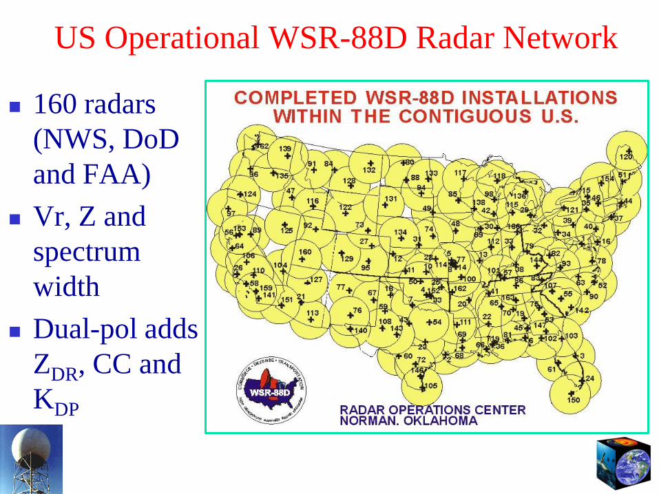
US Operational WSR-88D Radar Network

160 radars (NWS, DoD and FAA)

Vr, Z and spectrum width

Dual-pol adds ZDR, CC and KDP

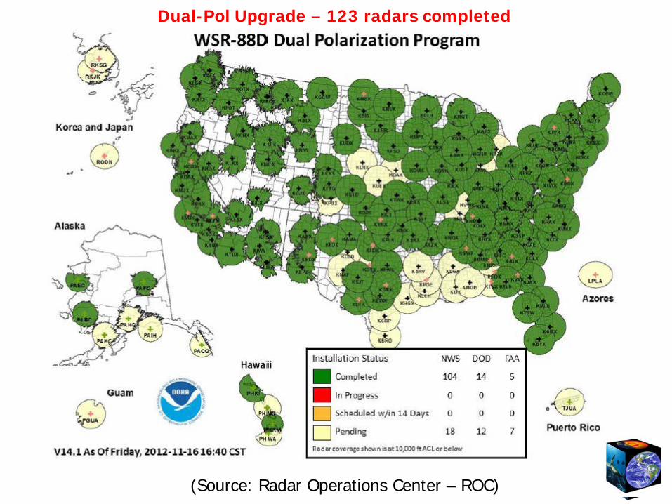
(Source: Radar Operations Center – ROC)

Dual-Pol Upgrade – 123 radars completed

Scanning Modes/ Data Volume

Clear air mode: 5 elevations (0.5-4.5º) /10 min

Precipitation modes: 14 elevations (0.5-19.5º) /5 mins

Maximum data volume: Z 250m in range up to 460 km, Vr 250 m in range up to 300 km, 0.5º in azimuth, up to 14 elevations, 1 volume scan/5 min 30 million observations/5 min for Vr and Z/radar.

Adding spectrum width, Zdr, CC, Kdp 90 million obs/5 min/radar.

160 radars 14 billion observations/5 min!

4 TB of data with 4:1 compression

The above is the worst case scenario – in reality, most radars run in clear air mode, and compression can be higher – 1 order of magnitude less.

Data Processing for Assimilation Data processing approaches:

Map the data from radar coordinates to model grid points (e.g., ARPS 3DVAR)

Map data in horizontal to model grid, but keep on elevations in the vertical (EnKF DA studies)

Keep data in radar coordinates (e.g., airborne radar) Further thinning to below grid resolution

QC critical, including velocity dealiasing. For large grids, parallel processing required.

Remapping/Data Thinning

Least square fitting on elevations for horizontal interpolation (88d2arps at in ARPS)

Cressman interpolation (VDRAS, etc.) Data selection based on variances (PSU?) Data every a few grid intervals

Main Methods of Radar Data Assimilation

3D variational (3DVAR) method

4D variational (4DVAR) method

Ensemble Kalman filter (EnKF) methods

Ensemble/Var hybrid methods

Semi-empirical methods, e.g., complex cloud analysis

Multi-step retrieval/analysis methods, e.g., Single-Doppler Velocity Retrieval (SDVR), thermodynamic retrieval techniques

Realtime Radar DA as Part of the CAPS Storm-Scale Ensemble Forecasting (SSEF)

for NOAA Hazardous Weather Test CAPS has been assimilating Level-2 Vr and Z data

from all WSR-88D radars into CONUS 1-4 km models using ARPS 3DVAR/Cloud analysis in realtime for HWT Spring Experiments since 2008.

The perturbed 3DVAR analyses were used to initialize up to 50 members of multi-model (4 models), multi-physics, multi-IC/LBC, storm-scale ensemble forecasts (SSEF) on a 4 km CONUS grid

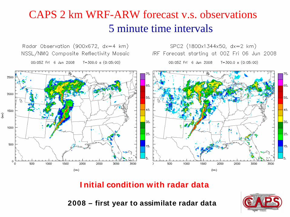
CAPS 2 km WRF-ARW forecast v.s. observations 5 minute time intervals

Initial condition with radar data

2008 – first year to assimilate radar data

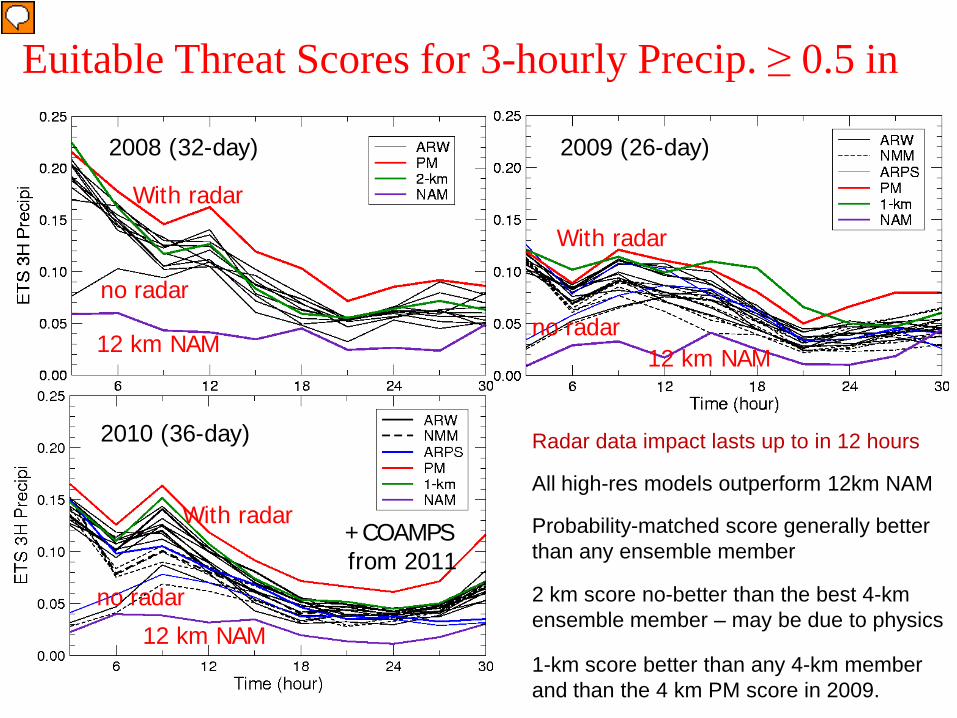
Euitable Threat Scores for 3-hourly Precip. ≥ 0.5 in

With radar

no radar 12 km NAM

2009 (26-day)

With radar

no radar

12 km NAM

2008 (32-day)

2010 (36-day) Radar data impact lasts up to in 12 hours

All high-res models outperform 12km NAM

Probability-matched score generally better than any ensemble member 2 km score no-better than the best 4-km ensemble member – may be due to physics 1-km score better than any 4-km member and than the 4 km PM score in 2009.

With radar

no radar

12 km NAM

+COAMPS from 2011

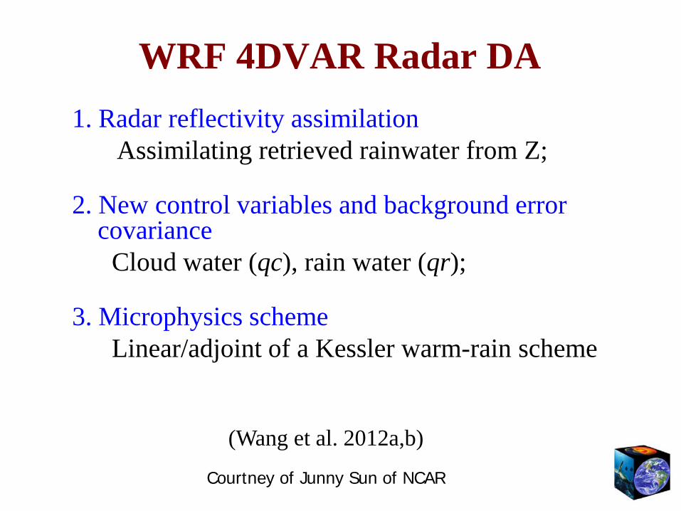
WRF 4DVAR Radar DA 1. Radar reflectivity assimilation Assimilating retrieved rainwater from Z; 2. New control variables and background error

covariance Cloud water (qc), rain water (qr); 3. Microphysics scheme Linear/adjoint of a Kessler warm-rain scheme

(Wang et al. 2012a,b)

Courtney of Junny Sun of NCAR

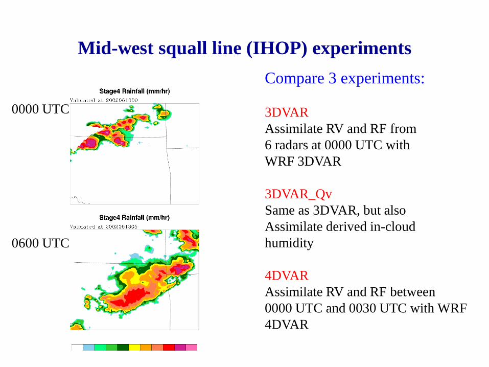
Mid-west squall line (IHOP) experiments Compare 3 experiments: 3DVAR Assimilate RV and RF from 6 radars at 0000 UTC with WRF 3DVAR 3DVAR_Qv Same as 3DVAR, but also Assimilate derived in-cloud humidity 4DVAR Assimilate RV and RF between 0000 UTC and 0030 UTC with WRF 4DVAR

0000 UTC

0600 UTC

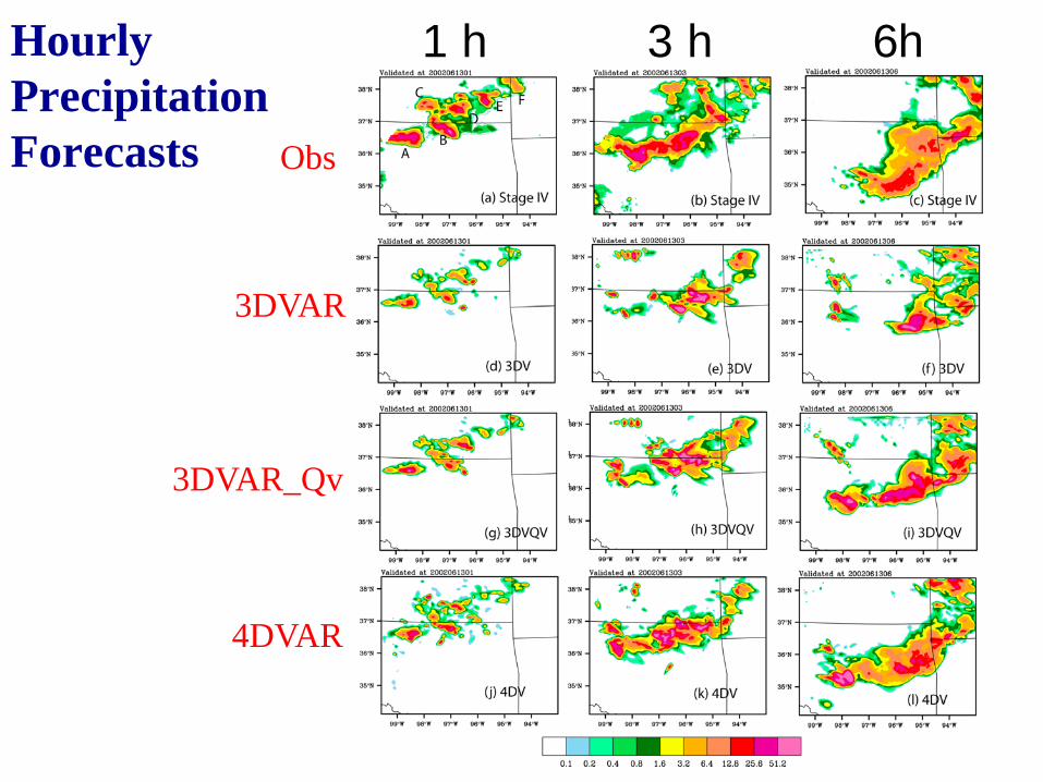
Hourly Precipitation Forecasts Obs

3DVAR

3DVAR_Qv

4DVAR

1 h 3 h 6h

EnKF Radar DA Examples

A Mesoscale Convective System that Spawned Several Tornadoes in

Oklahoma

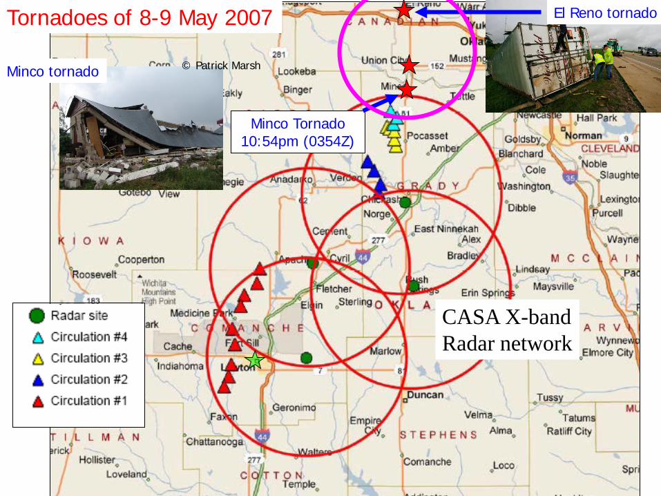
© Patrick Marsh

Minco Tornado 10:54pm (0354Z)

Tornadoes of 8-9 May 2007 El Reno tornado

Minco tornado

CASA X-band Radar network

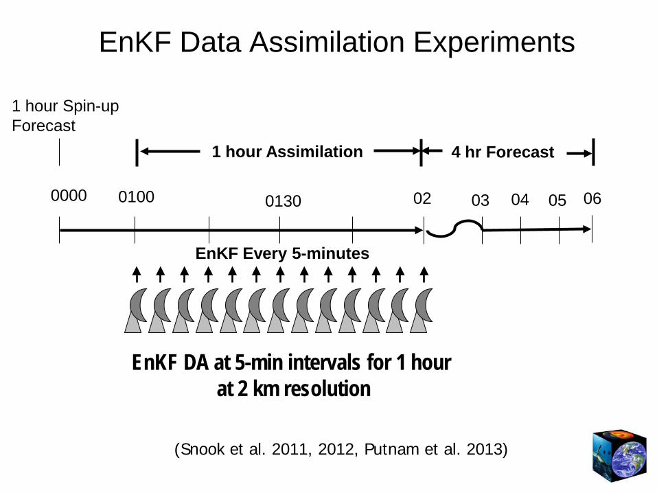
EnKF Data Assimilation Experiments

06 02

EnKF Every 5-minutes

03 04 05

4 hr Forecast 1 hour Assimilation

0000

EnKF DA at 5-min intervals for 1 hour at 2 km resolution

0100

1 hour Spin-up Forecast

0130

(Snook et al. 2011, 2012, Putnam et al. 2013)

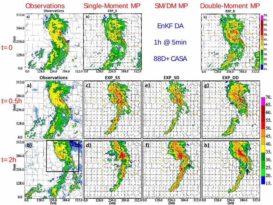
t=0

t=0.5h

t=2h

Observations Single-Moment MP SM/DM MP Double-Moment MP

EnKF DA

1h @ 5min

88D+CASA

EnKF Analysis of Dual-Pol Variables

Z ZDR KDP

Single moment

Double moment

Putnam et al (2013)

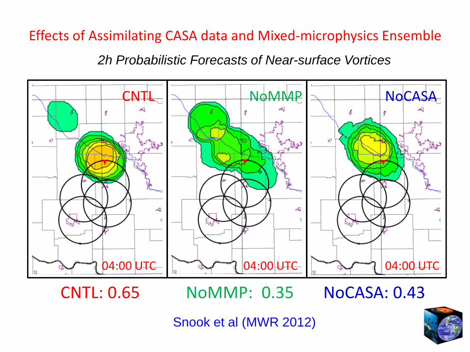
Effects of Assimilating CASA data and Mixed-microphysics Ensemble

2h Probabilistic Forecasts of Near-surface Vortices

CNTL NoCASA NoMMP

04:00 UTC 04:00 UTC 04:00 UTC

CNTL: 0.65 NoMMP: 0.35 NoCASA: 0.43 Snook et al (MWR 2012)

Parallel EnKF Algorithms • Dense Radar data on large high-res domains require

effective parallelization

• Radar DA has so far exclusively used serial EnSRF/EnAF algorithms

• LETKF easier to parallelize, but algorithm itself more expensive

• DART and GSI-based EnSRF parallelize on state vector level but still process one observation after another – hard to scale to high data volumes

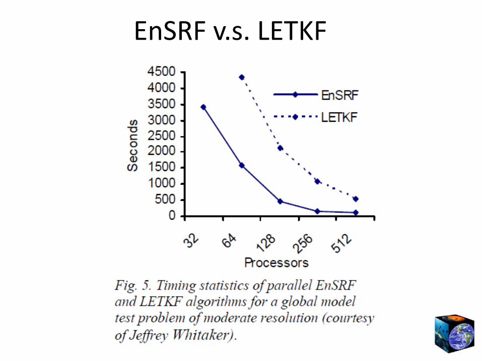
EnSRF v.s. LETKF

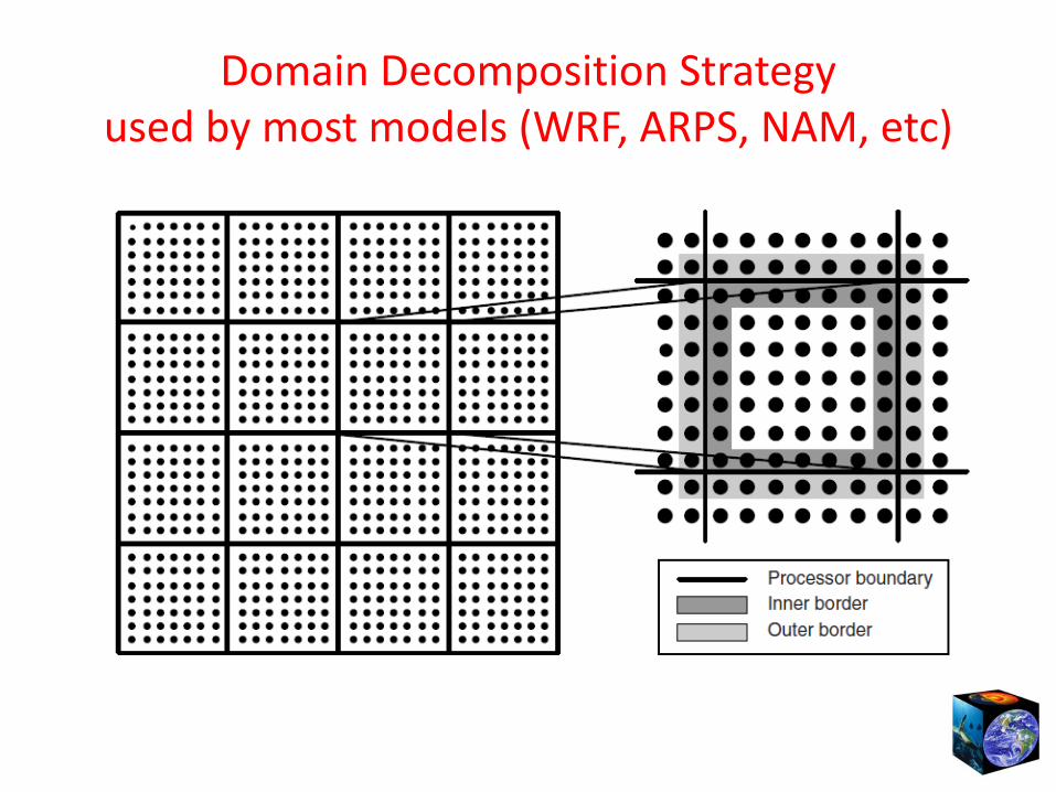
Domain Decomposition Strategy used by most models (WRF, ARPS, NAM, etc)

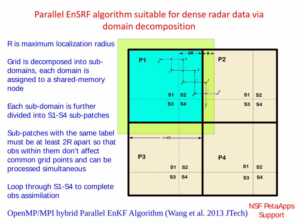
Parallel EnSRF algorithm suitable for dense radar data via domain decomposition

OpenMP/MPI hybrid Parallel EnKF Algorithm (Wang et al. 2013 JTech)

R is maximum localization radius Grid is decomposed into sub-domains, each domain is assigned to a shared-memory node Each sub-domain is further divided into S1-S4 sub-patches Sub-patches with the same label must be at least 2R apart so that obs within them don’t affect common grid points and can be processed simultaneous Loop through S1-S4 to complete obs assimilation NSF PetaApps

Support

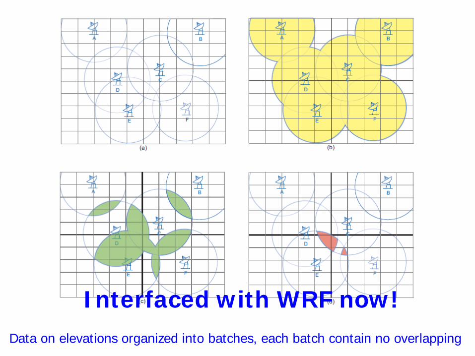
Data on elevations organized into batches, each batch contain no overlapping

Interfaced with WRF now!

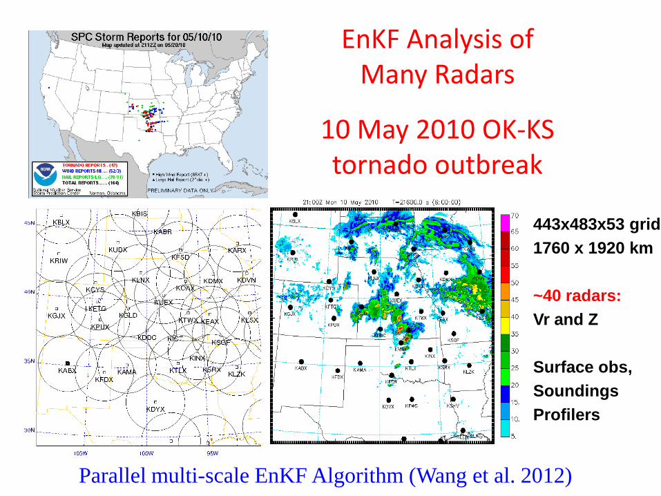
443x483x53 grid 1760 x 1920 km ~40 radars: Vr and Z

Surface obs, Soundings Profilers

EnKF Analysis of Many Radars

10 May 2010 OK-KS tornado outbreak

Parallel multi-scale EnKF Algorithm (Wang et al. 2012)

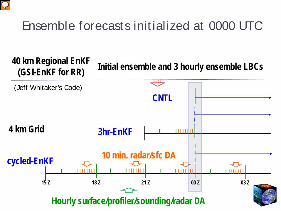
Hourly surface/profiler/sounding/radar DA

15 Z 18 Z 21 Z 00 Z

10 min. radar/sfc DA

03 Z

40 km Regional EnKF (GSI-EnKF for RR)

Ensemble forecasts initialized at 0000 UTC

cycled-EnKF

3hr-EnKF

CNTL

4 km Grid

Initial ensemble and 3 hourly ensemble LBCs

(Jeff Whitaker’s Code)

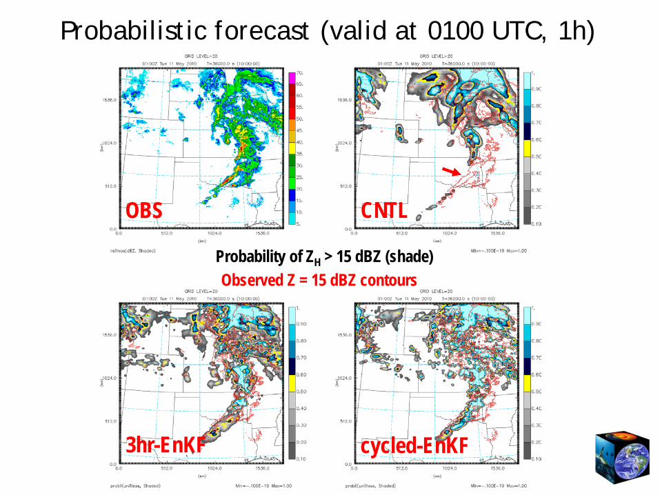
Probabilistic forecast (valid at 0100 UTC, 1h)

OBS CNTL

3hr-EnKF cycled-EnKF

Probability of ZH > 15 dBZ (shade) Observed Z = 15 dBZ contours

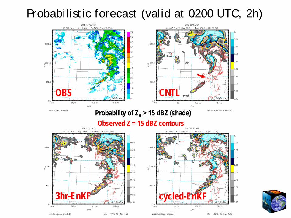
Probabilistic forecast (valid at 0200 UTC, 2h)

OBS CNTL

3hr-EnKF cycled-EnKF

Probability of ZH > 15 dBZ (shade) Observed Z = 15 dBZ contours

Probabilistic forecast (valid at 0300 UTC, 3h)

OBS CNTL

3hr-EnKF cycled-EnKF

Probability of ZH > 15 dBZ (shade) Observed Z = 15 dBZ contours

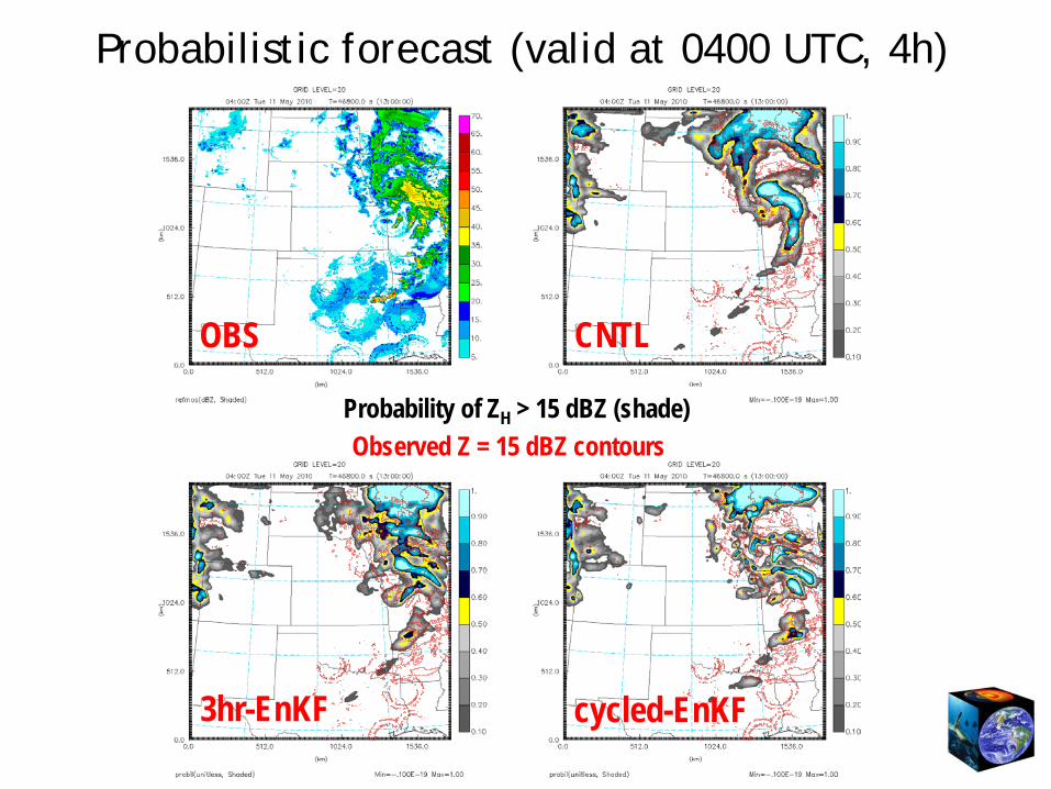
Probabilistic forecast (valid at 0400 UTC, 4h)

OBS CNTL

3hr-EnKF cycled-EnKF

Probability of ZH > 15 dBZ (shade) Observed Z = 15 dBZ contours

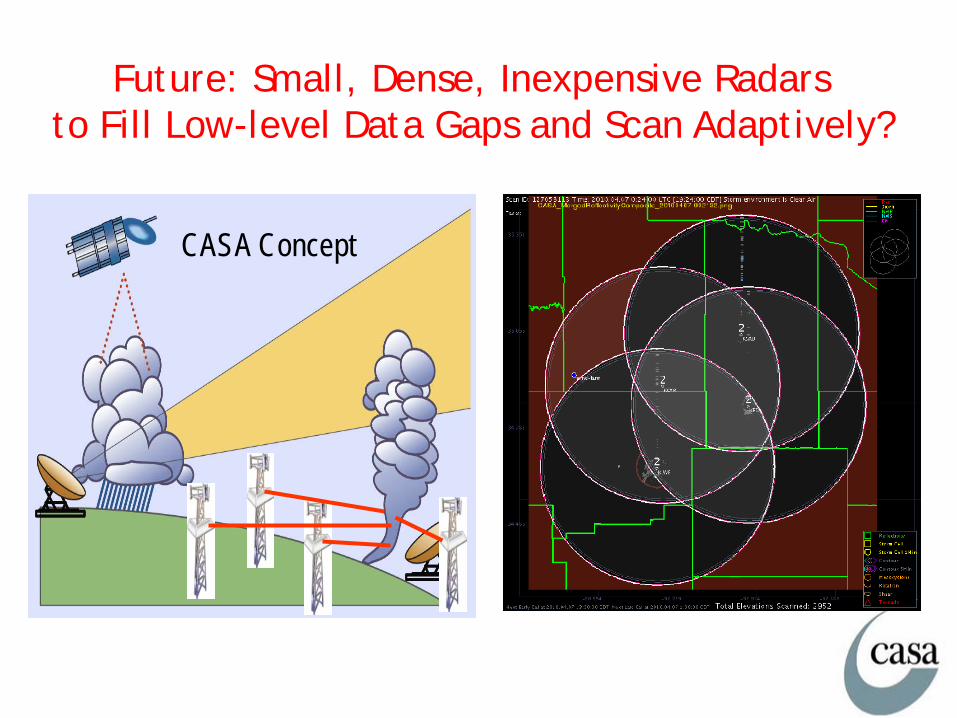
Future: Small, Dense, Inexpensive Radars to Fill Low-level Data Gaps and Scan Adaptively?

CASA Concept

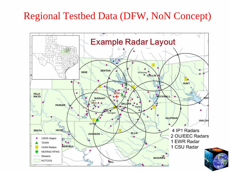
Regional Testbed Data (DFW, NoN Concept)

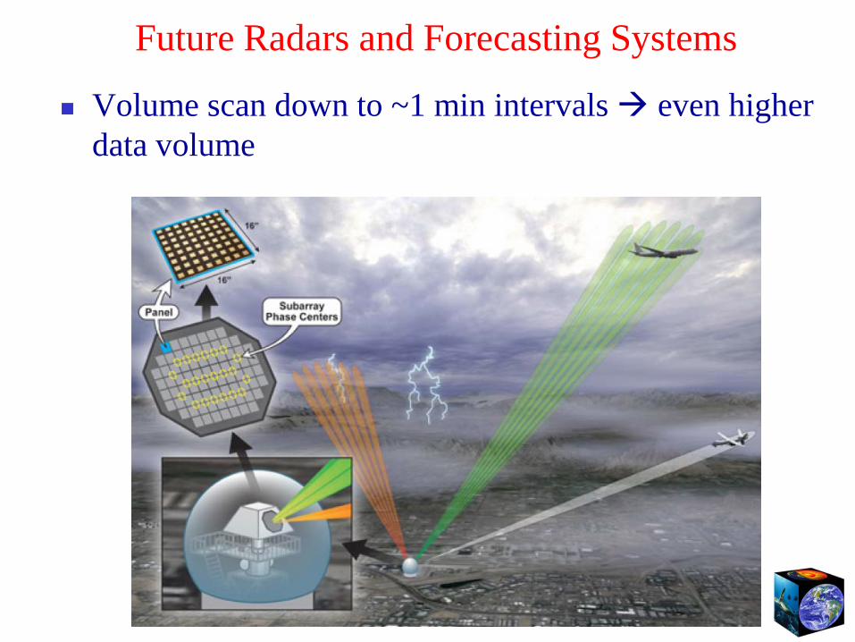
Future Radars and Forecasting Systems

Volume scan down to ~1 min intervals even higher data volume

Convection-Resolving Ensemble DA and Forecasting Need to integrate radar with all other data sources (conventional,

satellite, other remote sensing platforms) – multi-scale problem! Continuously cycled EnKF/Hybrid DA @ 5 min intervals @ 1-4 km

grid spacing CONUS+ domain 1-4 km ensemble forecasts updated every hour

(not ECMWF problem) Data ingest, processing, storage, distribution, analysis and

visualization all very challenging, more so for fast severe weather. Many research questions – Fuqing gave a very good list.

QC, model error, multi-scale issues

CAPS alone has produced several PB of data over the past 6 years – sitting inside mass storage systems – need something like Earthcube to liberate them!

Need orders of magnitude more resources and infrastructures to achieve the above goals.

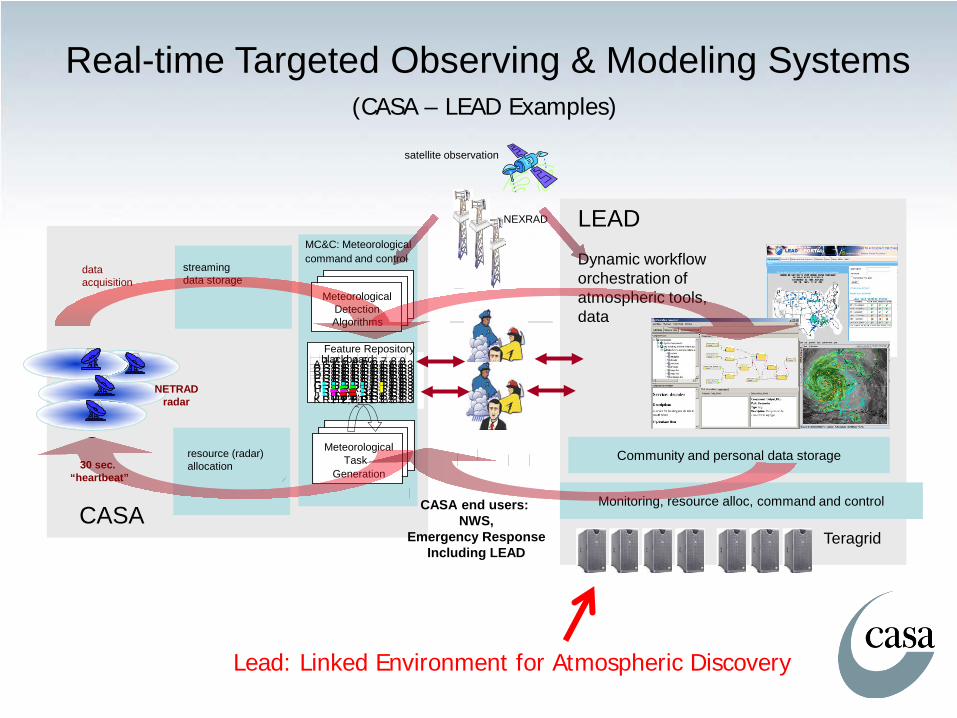
Real-time Targeted Observing & Modeling Systems

Meteorological Detection Algorithms

1 2 3 4 5 6 7 8 9 A G3 G3 G3 G3 G3 G3 G3 G3 G3 B G3 G3 G3 G3 G3 G3 G3 G3 G3 C G3 G3 G3 G3 G3 G3 G3 G3 G3 D G3 G3 G3 G3 G3 G3 G3 G3 G3 E G3 G3 G3 G3 G3 G3 G3 G3 G3 F G3 G3 G3 G3 G3 G3 G3 G3 G3 G G3 G3 G3 G3 G3 G3 G3 G3 G3 H R1 R1 R2 R2 R1 G3 C2 G3 G3 I R1 F 1 F 2, R1 F 2,H2 R1 G3 C2 G3 G3 J R1 H1 , F1 H1 , F1 T 2,R1 R1 G3 C2 G3 G3 K R1 H1 T 2,H1 T 2,R1 R1 G3 G3 G3 G3

Feature Repository

MC&C: Meteorological command and control

Meteorological Task

Generation

blackboard

streaming data storage

resource (radar) allocation 30 sec.

“heartbeat”

data acquisition

NETRAD radar

CASA

satellite observation

NEXRAD

Community and personal data storage

Monitoring, resource alloc, command and control

Dynamic workflow orchestration of atmospheric tools, data

LEAD

Teragrid

CASA end users: NWS,

Emergency Response Including LEAD

Lead: Linked Environment for Atmospheric Discovery

(CASA – LEAD Examples)

Thanks!